Correlation decay and large deviations for mixed systems

Abstract

We consider low–dimensional dynamical systems with a mixed phase space and discuss the typical appearance of slow, polynomial decay of correlations: in particular we emphasize how this mixing rate is related to large deviations properties.

1 Introduction

In this contribution we plan to provide a short review of results concerning mixing properties of deterministic dynamical systems. In particular our emphasis will be on systems enjoying ergodicity in the conventional sense[1, 2], and not infinite ergodicity[3], where the very concept of mixing turns out to be quite delicate[4, 5]. The general idea is that when some deterministic dynamics presents a mixed phase space, namely coexistence of a chaotic sea with (even arbitrarily small) regular structures, sticking of a typical trajectory close to regular zones enhances severely correlations, and generically the speed of mixing becomes polynomial, where instead, for a fully chaotic system we expect exponential decay of correlations. In what follows we will denote by weakly chaotic systems those for which a power-law decay of correlations is indeed present. We emphasise that, beyond the simple “mathematical” examples we will mention in the next section, the general observations still apply to non trivial physical settings, notably in fluid dynamics[6, 7, 8].

2 Weak chaos

Here we provide a number of examples of the kind of systems our analysis is devoted to: simplest examples involve one dimensional dynamics. Here the prototype case is represented by Pomeau-Manneville map[9],

$$x_{n+1}=T_{PM}(x_{n})=\left.x_{n}+x_{n}^{z}\right|_{mod\,\,1},$$ (1)

which presents an extremely reach behaviour as the intermittency parameter $z$ is varied. At $z=1$ it coincides with Bernoulli map, the standard example of fully chaotic (uniformly hyperbolic dynamics), but as soon as $z>1$ the $0$ fixed point becomes marginal, the invariant measure develops a singularity at the origin, and anomalous features appear[10, 11]. When $z\geq 2$ the singularity of the invariant measure at the origin becomes non integrable, and (1) provides one of the simplest examples of infinite ergodicity[12, 13]. In the regime $1<z<2$ the system is ergodic (the invariant probability measure will be denoted by $\mu$), and displays power-law decay of correlation functions: in particular Hu[14] proved that there exist Lipschitz functions $F$ and $G$ such that

$$\left|\int_{I}\,d\mu\,(F\circ T_{PM}^{n})G-\int_{I}\,d\mu\,F\,\int_{I}\,d\mu\,G\right|=O(n^{-\xi}),$$ (2)

where the exponent $\xi_{PM}$ is determined by the intermittency parameter $z$ through

$$\xi_{PM}=\frac{1}{z-1}-1.$$ (3)

In particular one notices that $\xi_{PM}$ diverges in the Bernoulli limit $z\to 1^{+}$, while for $z\geq 3/2$ correlations are not integrable, the standard central limit theorem does not hold and properly renormalized Birkhoff averages converge to a Lévy stable law[15]. We remark that in this example the “regular” region amounts only on the indifferent fixed point at the origin.
Another well known example is provided by Pikovsky map $T_{P}$ [16] (see [17] for more detailed bibliography), which is implicitly defined by

$$x=\left\{\begin{array}[]{ll}\displaystyle\frac{1}{2z}[1+T_{P}(x)]^{z},\hskip 45.52458pt0<x<1/(2z),\\ T_{P}(x)+\displaystyle\frac{1}{2z}[1-T_{P}(x)]^{z},\hskip 8.5359pt1/(2z)<x<1;\end{array}\right.$$ (6)

while for negative values of $x\in[-1,0]$, the map is defined as $T_{P}(-x)=-T_{P}(x)$. A remarkable feature of $T_{P}$ is that, while retaining indifferent fixed points (at $x=\pm 1$) with an intermittency parameter $z$, the invariant probability measure $\mu$ is the Lebesgue measure (it is a simple exercise to verify that by writing down the corresponding Perron-Frobenius operator): this is obtained by letting the instability unbounded close to the origin. Again we have a polynomial decay rate for correlations, with

$$\xi_{P}=\frac{1}{z-1};$$ (7)

here any value of $z>1$ is allowed, and correlations become non integrable (with a generalized central limit theorem[17]) for $z\geq 2$.
Examples of similar behaviour in hamiltonian dynamics include billiard tables in two dimensions, like the stadium or Sinai billiard (see for instance [18]), the limit of kissing discs for diamond billiards[19, 20]  , or mushroom billiards[21].
Another popular context is that of area-preserving maps, where the prototype example is the so called standard map [22, 23]:

$$S_{(K)}:\left\{\begin{array}[]{ll}y_{n+1}=y_{n}-K\sin(x_{n})&\mathrm{mod}\,2\pi,\\ x_{n+1}=x_{n}+y_{n+1}&\mathrm{mod}\,2\pi.\end{array}\right.$$ (10)

Despite the simple structure of (10), rigorous analysis of the standard map is extremely difficult[26], and the structure of regular regions, where typical orbits stick for a long time, causing slow correlation decay, is extremely rich (see for example [27, 28, 29]). There is a class of different area-preserving maps with a simpler phase space structure:

$$L_{(\varepsilon,\gamma)}:\left\{\begin{array}[]{ll}y_{n+1}=y_{n}+f(x_{n})&\mathrm{mod}\,2\pi,\\ x_{n+1}=x_{n}+y_{n+1}&\mathrm{mod}\,2\pi,\end{array}\right.$$ (13)

where $f(x_{n})$ is defined by

$$f(x_{n})=[x_{n}-(1-\varepsilon)\sin(x_{n})]^{\gamma}.$$ (14)

Such a map was introduced in [30], for $\varepsilon=0$ and $\gamma=1$, and generalized in [31, 32], where a transition to polynomial decay of correlations was observed as $\varepsilon\to 0^{+}$. As a matter of fact for $\varepsilon>0$ the map is fully hyperbolic (and displays exponential correlations decay), while, for $\varepsilon=0$ the fixed point at $(0,0)$ becomes parabolic, playing a role analogous to the origin in Pomeau-Manneville maps (and $\gamma$ is a sort of intermittency exponent). By considering the dynamics along the unstable manifold, in [32] is was argued that the correlation decay for $\varepsilon=0$ is polynomial, with

$$\xi_{L}=\frac{3(\gamma+1)}{3\gamma-1};$$ (15)

this in particular predicts an exponent $\xi_{L}=3$ when $\gamma=1$: for such a parameter value there is a rigorous lower bound[34] $\xi_{L}\geq 2$.

3 Indirect approach to correlations: recurrences

Direct numerical investigations of correlation functions are notoriously hard to accomplish, since, even if the ergodic invariant measure is known (like in the case of area-preserving maps), a Monte Carlo computation of correlation functions with $N_{MC}$ points involves an error proportional to $1/\sqrt{N_{MC}}$, which causes huge fluctuations after moderate times.
An indirect approach, which has been widely used in the last decades, involves recurrence time (Poincaré) statistics. Such an approach was pioneered in [35, 24, 25], and it admits a rigorous basis[36] (see also [37]). We briefly describe a simple version of it[24]: suppose we partition the phase space into two disjoint subsets, labelled $0$ and $1$: from a long trajectory of the system we extract the sequence of residence times $n_{1},n_{2},\dots,n_{k},\dots$ (for simplicity we are considering a discrete time dynamics) on a single subset (namely the waiting times before crossing the border). This leads to a probability distribution for residence times $\wp(n)$: we also suppose that the average residence time $\nu=\langle n\rangle=\sum\,k\cdot\wp(k)$ is finite. Now we make the (severe) hypothesis that crossing the border leads to a complete decorrelation of the dynamics[38, 39]: in this way[40], if we consider the autocorrelation function of an observable $G$:

$$C_{GG}(m)=\langle G(m_{0}+m)G(m_{0})\rangle-\langle G\rangle^{2},$$ (16)

we have that $\langle G(m_{0}+m)G(m_{0})\rangle=\langle G^{2}\rangle$ if no crossing takes place between $m_{0}$ and $m_{0}+m$ and $\langle G(m_{0}+m)G(m_{0})\rangle=\langle G\rangle^{2}$ otherwise. If we denote by $\Pi(m)$ the probability that no crossing took place in the time lapse $[m_{0},m_{0}+m]$, then

$$C_{GG}(m)=\Pi(m)\langle G^{2}\rangle+(1-\Pi(m))\langle G\rangle^{2}-\langle G\rangle^{2}=\Pi(m)\left(\langle G^{2}\rangle-\langle G\rangle^{2}\right).$$ (17)

Now it is easy to express $\Pi(m)$ in terms of $\wp(k)$, since the probability that a point chosen at random is the first point of a residence sequence of length $k$ is $\wp(k)/\nu$ while the probability that a point chosen at random is the first, or the second, of a $k+1$ residence sequence is $\wp(k+1)/\nu$: thus:

$$\Pi(m)=\frac{1}{\nu}\left(\wp(m)+2\cdot\wp(m+1)+3\cdot\wp(m+2)+\cdots\right)=\frac{1}{\nu}\sum_{j=m}^{\infty}\,\sum_{i=j}^{\infty}\,\wp(i).$$ (18)

In this way, an exponential decay of $\wp(m)$ yields a similar exponential decay for correlation functions, while a power-law decay $\wp(m)\sim m^{-\alpha}$ corresponds to a polynomial correlation decay, with $\xi=\alpha-2$: such a quantitative correspondence has been scrutinized in [20] for a number of billiard systems, in full agreement with known rigorous results (see for instance [41]). We remark again that the crucial approximation involved in the above reasoning consists in assuming decorrelation at each crossing: for a different kind of time statistics (flight times between collisions in a Lorentz gas with infinite horizon) such an hypothesis has been investigated in detail[40]: for short times it obviously misses features of real correlations (for instance multiple collisions between neighbouring discs), while it accurately reproduces the asymptotic regime.

4 Indirect approach to correlations: large deviations

The fundamental idea, at a qualitative level, is that the same dynamical mechanism that slows down correlation decay is responsible for anomalous (broad) distributions of finite time averages: in particular many studies have concerned features of distribution functions of finite-time Lyapunov exponents[27, 42, 43, 44, 45, 46]. A rigorous approach was proposed in[47] (see also [48, 49]): take a one-dimensional map $T$, then finite-time Lyapunov exponents are defined as

$$\lambda_{n}(x_{0})=\frac{1}{n}\ln\left|\left.\frac{dT^{(n)}(x)}{dx}\right|_{x_{0}}\right|.$$ (19)

Such finite time estimates generically depend upon the initial condition $x_{0}$, so they are characterized by a probability distribution $P_{n}(\lambda_{n})$, which, for ergodic and chaotic systems, collapses to a delta distribution in the asymptotic limit

$$\lim_{n\to\infty}P_{n}(\lambda_{n})=\delta(\lambda-\overline{\lambda}),$$ (20)

where $\overline{\lambda}$ is the Lyapunov exponent of the map $T$. If we fix a threshold $\tilde{\lambda}<\overline{\lambda}$, and compute the sub-threshold weights:

$${\cal M}_{\tilde{\lambda}}(n)=\int_{-\infty}^{\tilde{\lambda}}\,d\lambda_{n}\,P_{n}(\lambda_{n})$$ (21)

we have that such quantities vanish in the large time limits, however their decay is related to correlation decay: more precisely the rigorous result in [47] states that, indipendently of the choice of the threshold $\tilde{\lambda}$, if

$${\cal M}_{\tilde{\lambda}}(n)\sim\frac{1}{n^{\sigma}},$$ (22)

then correlation functions of smooth observables satisfy the bound

$$C(m)\leq\frac{1}{m^{\sigma-1}},$$ (23)

i.e. $\xi_{T}\geq\sigma-1$. Such a bound cannot be however optimal, as for Pomeau-Manneville maps a simple argument[50] shows that $\xi_{PM}=\sigma$.
We notice that an assessment like (22) is a (non-exponential) large deviation estimate (see for instance [51]), and as a matter of fact the most general results[52, 53, 54] can be stated as follows: if we consider a map $T$, such that $\xi_{T}$ is the power law mixing rate, than Birkhoff sums of an observable $\psi$ satisfy the following estimate:

$$\mu\left(x:\left|\frac{1}{n}\sum_{j=0}^{n-1}\psi(T^{(j)}(x))-\int\,d\mu\,\psi\right|>\epsilon\right)\leq C_{\psi,\epsilon}\frac{1}{n^{\xi_{T}}};$$ (24)

that is polynomial large deviations, with an exponent independent of the threshold, and coinciding with the one ruling correlations decay. In one dimension (24) includes the case of finite-time Lyapunov exponents (21), with $\psi(x)=\ln|T^{\prime}(x)|$, while in higher dimensions the leading finite-time Lyapunov exponent cannot be written as a simple Birkhoff sum: nevertheless it still represents a natural indicator.
Such a technique has been used in a variety of context[55]: from one dimensional maps as (6), to area preserving maps (13), and it has been also employed to corroborate universality claims[56] for correlation decay of area preserving maps with mixed phase space. More recently this method was also used in exploring mixing properties of coupled intermittent maps[57].

5 A model example

To provide an illustration of the technique we described in the former section, we provide new numerical experiments on the family (13) of area-preserving maps. In particular we want to emphasize two aspects: the transition from chaotic $\varepsilon>0$ to intermittent $\varepsilon=0$ behavior, and how (24) offers an efficient numerical tool to compute exact (polynomial) mixing rates in the latter case.
In Fig. (1) we plot $P_{n}(\lambda_{n})$ for different cases: the hyperbolic case $(a)$ has been obtained by $5\cdot 10^{6}$ initial condition, while the intermittent case $(b)$ refers to $10^{7}$ initial conditions. One almost obvious feature is that when we go to $\varepsilon=0$ case the distributions look asymmetric, due to the frequent appearance of low estimates for Lyapunov exponents due to sticking to the parabolic fixed point. This leads to a quantitative analysis once we estimate how the subthreshold tail of the distributions shrinks to zero (21): in the hyperbolic case (Fig. (2 (a)), we observe a purely exponential decay (notice that the data referring to the case $\gamma=2$ have been shifted to avoid overlapping), as expected for a fully hyperbolic case, while in the parabolic $\varepsilon=0$ case, we observe a power law decay, which, in view of (24) should coincide with the mixing rate. A regression analysis yields for $\gamma=2$, ${\cal M}_{\tilde{\lambda}}(n)\sim n^{-1.80\pm 0.01}$, while (15) predicts $\xi_{L}=9/5$, and for $\gamma=3$ ${\cal M}_{\tilde{\lambda}}(n)\sim n^{-1.49\pm 0.04}$, while (15) predicts $\xi_{L}=3/2$, witnessing how large deviation analysis turns to be an extremely powerful tool in the numerical analysis of quantitative mixing properties of dynamical systems with weak chaotic properties.

6 Conclusions

We have reviewed indirect methods for the investigations of correlation decay for systems with mixed phase space, where sticking manifests in slow, polynomial mixing rates. Together with the popular use of Poincaré recurrences, we emphasize new techniques based on large deviations properties: we present in the last section novel calculations that corroborate the effectiveness of such a method, by computing polynomial mixing rates of a weakly chaotic area-preserving maps with very high precision.

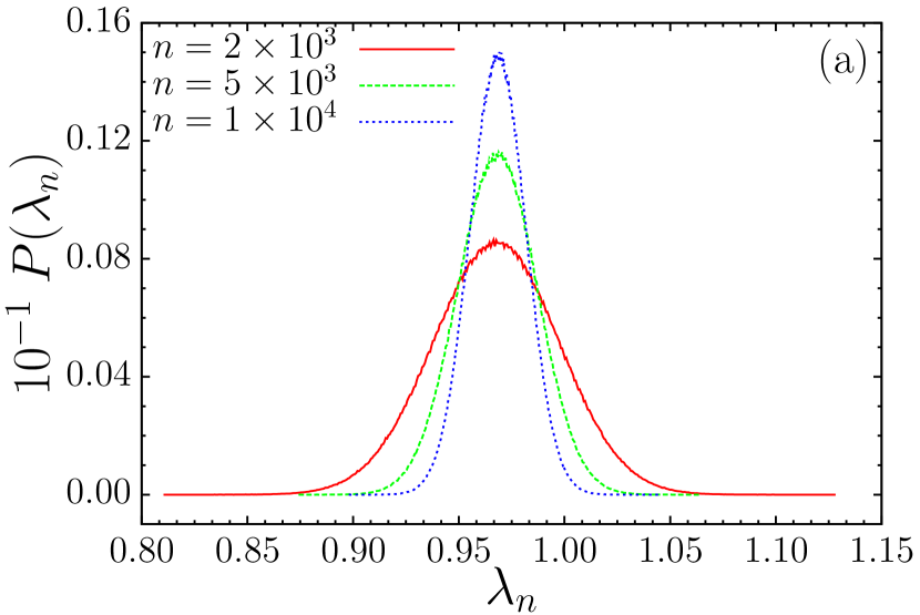
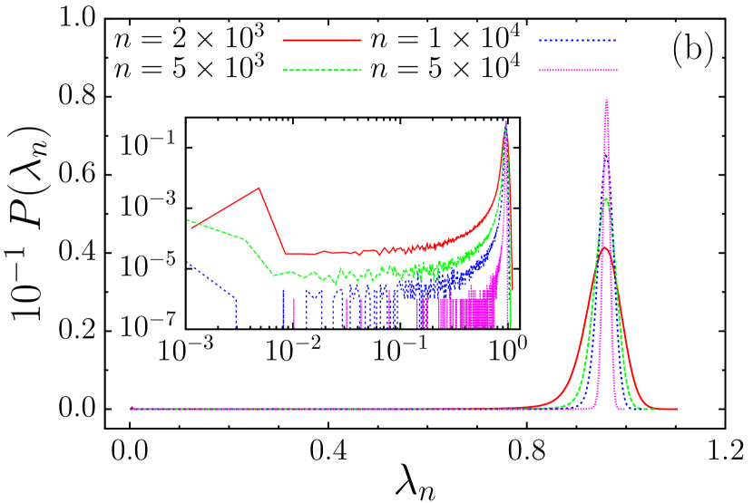
Figure 1: Distribution of finite-time maximal Lyapunov exponents for the map (13) with (a) $\varepsilon=1$ and $\gamma=2$ and (b) $\varepsilon=0$ and $\gamma=2$. (Inset: distributions of finite-time maximal Lyapunov exponents plotted in logarithm scale.)

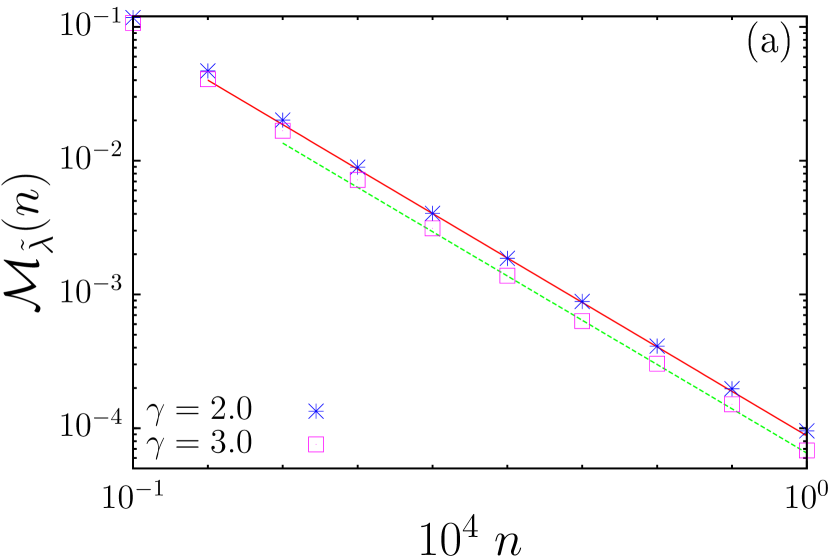
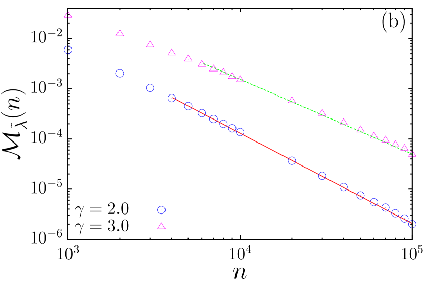
Figure 2: Decay $\mathcal{M}_{\tilde{\lambda}}(n)$ (symbols) together with a regression fit (full lines) for the map (13) with (a) $\varepsilon=1$ and $\gamma=2$ and $\gamma=3$ and (b) $\varepsilon=0$ and $\gamma=2$ and $\gamma=3$.

References

- [1] V. I. Arnold and A. Avez, Ergodic Problems of Classical mechanics, (Addison-Wesley, Reading, 1989).
- [2] I. P. Cornfeld, S. V. Fomin and Ya. G. Sinai, Ergodic theory, (Springer-Verlag, New York, 1982).
- [3] J. Aaronson, An Introduction to Infinite Ergodic Theory, (American Mathematical Society, Providence, 1997).
- [4] I. Melbourne and D. Terhesiu, Operator renewal theory and mixing rates for dynamical systems with infinite measure, Invent.Math. 189, 61 (2012).
- [5] M. Lenci, On infinite-volume mixing, Commun.Math.Phys. 298, 485 (2010).
- [6] P. Castiglione, A. Mazzino, P. Muratore-Ginanneschi, A. Vulpiani, On strong anomalous diffusion, Physica D 134, 75 (1999).
- [7] F. Raynal and P. Carrière, The distribution of “time of flight” in three dimensional stationary chaotic advection, Phys.Fluids 27, 043601 (2015).
- [8] T. H. Somolon and J. P. Gollub, Chaotic particle transport in time-dependent Rayleigh-Bénard convection, Phys.Rev. A 38, 6280 (1988).
- [9] Y. Pomeau and P. Manneville, Intermittent transition to turbulence in dissipative dynamical systems, Commun.Math.Phys. 2, 189 (1980).
- [10] P. Gaspard and X.-J. Wang, Sporadicity: between periodic and chaotic dynamical behaviors, Proc.Natl.Acad.Sci. USA 85, 4591 (1988).
- [11] X.-J. Wang, Statistical physics of temporal intermittency, Phys.Rev. A 40, 6647 (1989).
- [12] R. Zweimüller, Ergodic properties of infinite measure-preserving interval maps with indifferent fixed points, Ergod.Th. & Dynam.Sys. 20, 1519 (2000).
- [13] G. Bel and E. Barkai, Weak ergodicity breaking with deterministic dynamics, Europhys.Lett. 74, 15 (2006).
- [14] H. Hu, Decay of correlations for piecewise smooth maps with indifferent fixed points, Ergod.Th. & Dynam.Sys. 24, 495 (2004).
- [15] S. Gouëzel, Central limit theorem and stable laws for intermittent maps,Probability Theory and Related Fields 128, 82 (2004).
- [16] A. Pikovsky, Statistical properties of dynamically generated anomalous diffusion, Phys.Rev. A 43, 3146 (1991).
- [17] G. Cristadoro, N. Haydn, Ph. Marie and S. Vaienti, Statistical properties of intermittent maps with unbounded derivative, Nonlinearity, 23, 1071 (2010).
- [18] N. Chernov and R. Markarian, Chaotic billiards, (American Mathematical Society, Providence, 1996).
- [19] J. Machta, Power law decay of correlations in billiard problems, J.Stat.Phys. 32, 555 (1983).
- [20] R. Artuso, G. Casati and I. Guarneri, Numerical experiments in billiards, J.Stat.Phys. 83, 145 (1996).
- [21] L. A. Bunimovich, Mushrooms and other billiards with divided phase space, Chaos 11, 802 (2001).
- [22] B. V. Chirikov, A universal instability of many-dimensional oscillator systems, Phys.Rep. 52, 263 (1979).
- [23] A. J. Lichtenberg and M. A. Lieberman, Regular and chaotic dynamics, (Springer-Verlag, New York, 1992).
- [24] C. F.F. Karney, Long-time correlations in the stochastic regime, Physica D 8, 360 (1983).
- [25] B. V. Chirikov and D. L. Shepelyansky, Correlation properties in dynamical chaos in hamiltonian systems, Physica D 13, 395 (1984).
- [26] K. Bloor and S. Luzzatto, Some remarks on the geometry of the standard map, Int.J.Bif.Chaos 19, 2213 (2009).
- [27] S. Tomsovic and A. Lakshminarayan, Fluctuations of finite-time stability exponents in the standard map and the detection of small islands, Phys.Rev. E 76, 036207 (2007).
- [28] M. Sala, C. Manchein and R. Artuso, Estimating hyperbolicity of chaotic bidimensional maps, Int.J.Bifurc.Chaos 22, 1250217 (2012).
- [29] C. Manchein and M. W. Beims, Conservative generalized bifurcation diagrams, Phys.Lett. A 377, 789 (2013).
- [30] J. Lewowicz, Lyapunov functions and topological stability, J.Diff.Eq. 38, 192 (1980).
- [31] R. Artuso and A. Prampolini, Correlation decay for an intermittent area-preserving map, Phys.Lett. A 246, 407 (1988).
- [32] R. Artuso, L. Cavallasca and G. Cristadoro, Dynamical and transport properties in a family of intermittent area-preserving maps, Phys.Rev. E 77, 046206 (2008).
- [33] C. Liverani, Birth of an elliptic island in a chaotic sea, Math.Phys.El.J. 10, 1 (2004).
- [34] C. Liverani and M. Martens, Convergence to equilibrium for intermittent symplectic maps, Commun.Math.Phys. 260, 527 (2005).
- [35] S. R. Channon and J. L. Lebowitz, Numerical experiments in stochasticity and heteroclinic oscillation, Ann.N.Y.Acad.Sci. 357, 108 (1980).
- [36] L.-S. Young, Recurrence times and rates of mixing, Israel J.Math. 110, 153 (1999).
- [37] V. Baladi, Decay of correlations, Proc.Symposia Pure Math. 69, 297 (2001).
- [38] V. Baladi, J. P. Eckmann and D. Ruelle, Resonances for intermittent systems, Nonlinearity 2, 119 (1989).
- [39] P. Dahlqvist, Approximate zeta functions for the Sinai billiard and related systems, Nonlinearity 8, 11 (1995).
- [40] P. Dahlqvist and R. Artuso, On the decay of correlations in Sinai billiards with infinite horizon, Phys.Lett. A 219, 212 (1996).
- [41] L. A. Bunimovich, On the rate of decay of correlations in dynamical systems with chaotic behavior, Sov.Phys. JETP 62, 842 (1985).
- [42] M. Falcioni, U. Marini Bettolo Marconi and A. Vulpiani, Ergodic properties of high-dimensional symplectic maps, Phys.Rev. A 44, 2263 (1991).
- [43] H. Schomerus and M. Titov, Statistics of finite-time Lyapunov exponents in a random time-dependent potential, Phys.Rev. E 66, 066207 (2002).
- [44] C. Anteneodo, Statistics of finite-time Lyapunov exponents in the Ulam map, Phys.Rev. E 69, 016207 (2004).
- [45] M. W. Beims, C. Manchein and J. M. Rost, Origin of chaos in soft interactions and signatures of nonergodicity, Phys.Rev. E 76, 056203 (2007)
- [46] C. Manchein, M. W. Beims and J. M. Rost, Characterizing the dynamics of higher dimensional nonintegrable conservative systems, Chaos 22, 033137 (2012).
- [47] J. F. Alves, S. Luzzatto and V. Pinheiro, Lyapunov exponents and rates of mixing for one-dimensional maps, Ergod.Th. & Dynam.Sys. 24, 637 (2004).
- [48] J. F. Alves, S. Luzzatto and V. Pinheiro, Markov structures and decay of correlations for non-uniformly expanding dynamical systems, Ann.I.H. Poincaré AN22, 817 (2005).
- [49] J. F. Alves, J. M. Freitas, S. Luzzatto and S. Vaienti, From rates of mixing to recurrence times via large deviations, Adv.Math. 228, 1203 (2011).
- [50] R. Artuso and C. Manchein, Comment on “Lyapunov statistics and mixing rates”, Phys.Rev. E 87, 016901 (2013).
- [51] F. den Hollander, Large deviations, (American Mathematical Society, Providence, 2000).
- [52] I. Melbourne, Large and moderate deviations for slowly mixing dynamical systems, Proc.Am.Math.Soc. 137, 1735 (2009).
- [53] M. Pollicott and R. Sharp, Large deviations for intermittent maps, Nonlinearity 22, 2079 (2009).
- [54] I. Melbourne and M. Nicol, Large deviations for nonuniformly hyperbolic systems, Trans.Amer.Math.Soc. 360, 6661 (2008).
- [55] R. Artuso and C. Manchein, Instability statistics and mixing rates, Phys.Rev. E 80, 036210 (2009).
- [56] G. Cristadoro and R. Ketzmerick, Universality of algebraic decays in hamiltonian systems, Phys.Rev.Lett. 100, 184101 (2008).
- [57] M. Sala, C. Manchein and R. Artuso, Extensive numerical investigations on the ergodic properties of two coupled Pomeau-Manneville maps, Physica A 438, 40 (2015).