Elliptic solutions and solitary waves of a higher order KdV–BBM long wave equation

Abstract

We provide conditions for existence of hyperbolic, unbounded periodic and elliptic solutions in terms of Weierstrass $\wp$ functions of both third and fifth-order KdV–BBM (Korteweg-de Vries–Benjamin, Bona & Mahony) regularized long wave equation. An analysis for the initial value problem is developed together with a local and global well-posedness theory for the third-order KdV–BBM equation. Traveling wave reduction is used together with zero boundary conditions to yield solitons and periodic unbounded solutions, while for nonzero boundary conditions we find solutions in terms of Weierstrass elliptic $\wp$ functions. For the fifth-order KdV–BBM equation we show that a parameter $\gamma=\frac{1}{12}$, for which the equation has a Hamiltonian, represents a restriction for which there are constraint curves that never intersect a region of unbounded solitary waves, which in turn shows that only dark or bright solitons and no unbounded solutions exist. Motivated by the lack of a Hamiltonian structure for $\gamma\neq\frac{1}{12}$ we develop $H^{k}$ bounds, and we show for the non Hamiltonian system that dark and bright solitons coexist together with unbounded periodic solutions. For nonzero boundary conditions, due to the complexity of the nonlinear algebraic system of coefficients of the elliptic equation we construct Weierstrass solutions for a particular set of parameters only.

I Introduction

In a recent paper Carv , the authors have derived a second-order mathematical description of long-crested water waves propagating in one direction, which is analogous to a first-order approximation of a KdV–BBM-type equation, which has the advantage that its solutions are expected to be more accurate on a much longer time scale BCPS ; Carv .

The wave motion of crested waves propagate in the direction $x$, the bottom is flat with undisturbed depth $h_{0}$, the undisturbed and dependent variable is $u(x;t)=h(x;t)-h_{0}$, where $h(x;t)$ is the height of the water column at the horizontal location $x$ on the bottom at time $t$. The fact that the waves are long-crested is based on the assumption that the wave amplitudes and wavelengths are small and large as compared to the depth $h_{0}$ of the flat bottom. If $A$ is the amplitude of the wave with wave length $\lambda$ then $\alpha=A/h_{0}\ll 1$, $\beta=h_{0}^{2}/\lambda^{2}\ll 1$. The Stokes’ number $S=\alpha/\beta\approx 1$ means that the nonlinear and dispersive effects are balanced. The parameter $1/\alpha\approx 1/\beta$ is the so-called Boussinesq time for which models like BBM and KdV are known to provide good approximations of the unidirectional solutions of the full water wave problem 1a ; 15a ; 17a ; 18a ; 29a ; 30a . In ocean wave modeling, waves need to be followed on a time longer than Bousinesq time scale, and hence a higher order approximation to the water wave problem would be valid on the scale $1/\beta^{2}$.

In their description BCPS dissipation and surface tension are neglected, the fluid is incompressible and irrotational. The velocity field is provided by the Euler equations, and the boundary behavior by the Bernoulli condition. The starting point of their description was essentially the papers 13a ; 10a , where a variant of the Boussinesq coupled system was derived for both first and second order in the small parameters $\alpha,\beta$ for which the well-posedness of the Cauchy problem was studied in 10a ; 11a ; Bous ; Raz ; Chen2 . From the first-order system they derived the mixed third-order KdV–BBM type equation

$$u_{t}+u_{x}+\frac{3}{2}\alpha uu_{x}+\nu\beta u_{xxx}-\left(\frac{1}{6}-\nu\right)\beta u_{xxt}=0,$$ (I.1)

while from the second-order Boussinesq system they derived the unidirectional model, a mixed fifth-order KdV–BBM type equation

$$u_{t}+u_{x}-\frac{\beta}{6}u_{xxt}+\delta_{1}\beta^{2}\,u_{xxxxt}+\delta_{2}\beta^{2}u_{xxxxx}+\frac{3\alpha}{2}uu_{x}+\alpha\beta\gamma(u^{2})_{xxx}-\frac{1}{12}\alpha\beta({u_{x}}^{2})_{x}-\frac{1}{4}\alpha^{2}(u^{3})_{x}=0.$$ (I.2)

The small parameters $\alpha,\beta$ of both equations can be eliminated by reverting to non-dimensional form, denoted by tilde where $\tilde{x}=\frac{x}{\sqrt{\beta}}\,,\,\tilde{t}=\frac{t}{\sqrt{\beta}}$ and $u(x,t)=\frac{1}{\alpha}\tilde{u}(\tilde{x},\tilde{t})$ and by suppressing the tilde yields to

$$u_{t}+u_{x}+\frac{3}{2}uu_{x}+\nu u_{xxx}-\left(\frac{1}{6}-\nu\right)u_{xxt}=0,$$ (I.3)

for Eq. (I.1), and to

$$u_{t}+u_{x}-\frac{1}{6}u_{xxt}+\delta_{1}u_{xxxxt}+\delta_{2}u_{xxxxx}+\left(\frac{3}{4}u^{2}+\gamma(u^{2})_{xx}-\frac{1}{12}{u_{x}}^{2}-\frac{1}{4}u^{3}\right)_{x}=0,$$ (I.4)

for Eq. (I.2). Notice that Eq. (I.3) is the BBM equation when $\nu=0$ and the KdV equation when $\nu=\frac{1}{6}$. As it was explained in BCPS Eq. (I.3) can be derived by expanding the Dirichlet-Neumann operator 31 , but this does not guarantee that the dispersion relation obtained fits the full dispersion to the order of the terms being kept, nor does it guarantee that the resulting equation provides a well-posed problem. In Amb1 and Amb2 this technique was applied to a deep-water situation where the resulting system is Hamiltonian, while the initial-value problem for it is ill-posed.

Higher-order versions of the KdV equation are not unique. Near-identity transformations can be used to make the higher-order terms take any desired form, as shown by the authors of Kod ; Hira ; Fok ; Cos . Any second-order KdV equation can be mapped asymptotically to integrable versions in the KdV hierarchy, such as the KdV equation itself. The same issue is also well-known for internal waves, see Grim .

II Well-posedness and energy estimates

The local well-posedness of Eq. (I.3) is established in §II.1 using a contraction mapping type argument combined with multilinear estimates. The global well-posedness of Eq. (I.3) is established in §II.2 in the spaces $H^{s}$, $s\geq 1$ which relies on the local results with energy type estimates. The issue of global well-posedness for the fifth-order Eq. (I.4) is addressed in BCPS . There, the assumption that $\gamma=\frac{1}{12}$ plays a crucial role in obtaining a conserved quantity which is used in the proof of global well-posedness for Eq. (I.1). Higher-order equations may not be Hamiltonian, but this is easily remedied through such a near-identity transformation. Thus, the restriction that $\gamma=\frac{1}{12}$ in Eq. (I.4) in order for this equation to be Hamiltonian is well-known and the remedy is to make such a transformation. In §II.3 we focus our attention on the traveling wave reduction of Eq. (I.1), and show that traveling wave solutions lie in $H^{k}$ for $k\geq 1\in\mathbb{N}$ with no assumption on the parameter $\gamma$. For exact solutions on other types of KdV–BBM equations see Dut ; Man ; Nic ; Kud with all the references therein.

II.1 Local well-posedness

We are interested in the local well-posedness associated to the Cauchy problem (I.3) for an initial profile $u(x,0)=u_{0}(x)\in H^{s}(\mathbb{R})$. The local well-posedness for the fifth-order Eq. (I.4) is established in BCPS , and we follow these techniques in establishing the local well-posedness of the third-order Eq. (I.3).

Taking the Fourier transform of Eq. (I.3) about $x$ defined by $\widehat{{u}(\xi,t)}=\mathcal{F}\{u(x,t)\}=\frac{1}{\sqrt{2\pi}}\int_{\mathbb{R}}u(x,t)\,e^{-i\xi x}\,dx$ yields

$$\widehat{u}_{t}+i\xi\widehat{u}+\frac{3}{4}i\xi\widehat{u^{2}}-i\nu\xi^{3}\widehat{u}+\left(\frac{1}{6}-\nu\right)\xi^{2}\widehat{u_{t}}=0,$$ (II.1)

which gives

$$\left[\left(\frac{1}{6}-\nu\right)\xi^{2}+1\right]i\widehat{u_{t}}=\xi\left(1-\nu\xi^{2}\right)\widehat{u}+\frac{3}{4}\xi\widehat{u^{2}}.$$ (II.2)

We assume that $\nu<\frac{1}{6}$, therefore $\left(\frac{1}{6}-\nu\right)\xi^{2}+1$ is positive and we have the equivalent equation

$$i\widehat{u_{t}}=\frac{\xi\left(1-\nu\xi^{2}\right)}{\left(\frac{1}{6}-\nu\right)\xi^{2}+1}\widehat{u}+\frac{3\xi}{4\left[\left(\frac{1}{6}-\nu\right)\xi^{2}+1\right]}\widehat{u^{2}}.$$ (II.3)

Define the following Fourier multipliers $\phi(\partial_{x})$, $\psi(\partial_{x})$ based on their symbols

$$\widehat{\phi(\partial_{x})f}(\xi)=\phi(\xi)\widehat{f}(\xi),\;\;\widehat{\psi(\partial_{x})f}(\xi)=\psi(\xi)\widehat{f}(\xi),$$

where $\phi(\xi)=\frac{\xi\left(1-\nu\xi^{2}\right)}{\left(\frac{1}{6}-\nu\right)\xi^{2}+1}$, $\psi(\xi)=\frac{3\xi}{4\left[\left(\frac{1}{6}-\nu\right)\xi^{2}+1\right]}.$ We can now reformulate the Cauchy problem in the following form

$$\begin{cases}iu_{t}=\phi(\partial_{x})u+\psi(\partial_{x})u^{2}\\ u(x,0)=u_{0}(x),\\ \end{cases}$$ (II.4)

and we solve the associated linear problem

$$\begin{cases}iu_{t}=\phi(\partial_{x})u\\ u(x,0)=u_{0}(x),\\ \end{cases}$$ (II.5)

where the solution is given by $u(t)=S(t)u_{0}$ with $\widehat{S(t)u_{0}}=e^{-i\phi(\xi)t}\widehat{u_{0}}$ defined by its Fourier transform. Duhamel’s principle gives us the integral form of the IVP (II.4):

$$u(x,t)=S(t)u_{0}-i\int^{t}_{0}S(t-s)\psi(\partial_{x})u^{2}(x,s)ds.$$

The operator $S(t)$ is a unitary operator on $H^{s}$ for any $s\in\mathbb{R}$, $\left\|S(t)u_{0}\right\|_{H^{s}}=\left\|u_{0}\right\|_{H^{s}}$. The local existence is established via a contraction mapping argument for the space $C\left(\left[0,T\right];H^{s}\right).$ We next need an estimate for the quadratic term in Eq. (II.4).

Lemma 1

For any $s\geq 0$ there exists a constant $C=C_{s}$ such that the following inequality

$$\left\|\psi(\partial_{x})u^{2}\right\|_{H^{s}}\leq C_{s}\left\|u\right\|^{2}_{H^{s}},$$ (II.6)

holds for the operator $\psi(\partial_{x})$.

• The proof relies on a bilinear estimate, see Lemma 3.1 in BCPS .

With the above estimate, and $S(t)$ being a unitary operator we show that the operator

$$\Psi u(x,t)=S(t)u_{0}-i\int^{t}_{0}S(t-s)\psi(\partial_{x})u^{2}(x,s)ds,$$ (II.7)

defines a contraction mapping on a closed ball $\mathcal{B}_{r}$ with radius $r>0$ centered at the origin in $C\left(\left[0,T\right];H^{s}\right)$. First we show that $\Psi$ maps $\mathcal{B}_{r}$ to itself

$$\left\|\Psi u(x,t)\right\|_{H^{s}}\leq\left\|u_{0}\right\|_{H^{s}}+CT\left\|\psi(\partial_{x})u^{2}\right\|_{C([0,T];H^{s})}\leq\left\|u_{0}\right\|_{H^{s}}+CT\left\|u\right\|^{2}_{C([0,T];H^{s})}.$$

Since $u\in\mathcal{B}_{r}$ it follows that

$$\left\|\Psi u(x,t)\right\|_{H^{s}}\leq\left\|u_{0}\right\|_{H^{s}}+CTr^{2}.$$

In order for $\Psi$ to map $\mathcal{B}_{r}$ onto itself we choose $r=2\left\|u_{0}\right\|_{H^{s}}$ and $T=\frac{1}{4Cr}$.

Next, we show that $\Psi$ is a contraction under the same choices of $r$ and $T$ by considering

$$\Psi u(x,t)-\Psi v(x,t)=-i\int^{t}_{0}S(t-s)\psi(\partial_{x})(u^{2}-v^{2})(x,s)ds,$$ (II.8)

which gives

$$\left\|\Psi u(x,t)-\Psi v(x,t)\right\|_{C([0,T];H^{s})}\leq 2rCT\left\|u-v\right\|_{C([0,T];H^{s})}<\left\|u-v\right\|_{C([0,T];H^{s})}.$$ (II.9)

We summarize all of the above in the following theorem:

Theorem 1

For any $s\geq 1$, and given $u_{0}\in H^{s}(\mathbb{R})$, there exists a time $T=T(\left\|u_{0}\right\|_{H^{s}})$, and a unique function $u\in C([0,T],H^{s})$ which is a solution to the IVP (I.3) with initial data $u_{0}$. The solution has continuous dependence on $u_{0}$ in $H^{s}(\mathbb{R})$.

Corollary 1

The following properties of $u(x,t)$ follow from the proof of Theorem 1.

1. The maximal existence time $T=T_{s}$ of the solution satisfies

   $$T\geq\tilde{T}=\frac{1}{4C_{s}\left\|u_{0}\right\|_{H^{s}}}.$$ (II.10)

2. We can bound the $H^{s}$ norm of the solution,

   $$\left\|u(\cdot,t)\right\|_{H^{s}}\leq r=2\left\|u_{0}\right\|_{H^{s}}$$

   for all $t\in[0,\tilde{T}]$ where $\tilde{T}$ is defined in (II.10).

II.2 Global well-posedness

The goal of this subsection is to extend the local well-posedness established in §II.1 for Eq. (I.3), and we derive energy estimates to obtain a global well-posedness result in $H^{s}(\mathbb{R})$ for $s\geq 1$. From the local theory the solution is only as smooth as the initial data, but one can make computations with smoother solutions and then pass to the limit of rougher initial data using the continuous dependence result by BK . Multiplying Eq. (I.3) by $u$ and integrating by parts over the spatial variable $x$ we obtain

$$\frac{1}{2}\frac{d}{dt}\int_{\mathbb{R}}\left[u^{2}+\left(\frac{1}{6}-\nu\right){u_{x}}^{2}\right]dx=-\left[\frac{1}{2}u^{2}+\frac{1}{2}u^{3}+\nu\left(uu_{xx}-\frac{1}{2}{u_{x}}^{2}\right)\right]\Bigg{|}_{\mathbb{R}}.$$ (II.11)

Therefore, if we assume that $u,\,u_{x},\,u_{xx}\rightarrow 0$ as $|x|\rightarrow\infty$, the energy of the third-order equation which is a conserved quantity is

$$E_{3}\big{(}u(\cdot,t)\big{)}=\frac{1}{2}\int_{\mathbb{R}}\left[u^{2}+\left(\frac{1}{6}-\nu\right){u_{x}}^{2}\right]dx=const,$$ (II.12)

and for $\nu<\frac{1}{6}$ this is equivalent to the $H^{1}$ norm of $u$. It is worth noting that a similar conserved quantity can be derived for Eq. (I.4), again by using parts to obtain

$$\frac{1}{2}\frac{d}{dt}\int_{\mathbb{R}}\left[u^{2}+\frac{1}{6}{u_{x}}^{2}+\delta_{1}{u_{xx}}^{2}\right]dx=\left(\gamma-\frac{1}{12}\right)\int_{\mathbb{R}}{u_{x}}^{3}dx,$$ (II.13)

so the energy is conserved when $\gamma=\frac{1}{12}$, whereas the energy of the fifth-order equation is

$$E_{5}\big{(}u(\cdot,t)\big{)}=\frac{1}{2}\int_{\mathbb{R}}\left[u^{2}+\frac{1}{6}{u_{x}}^{2}+\delta_{1}{u_{xx}}^{2}\right]dx=const.$$ (II.14)

For $\gamma=\frac{1}{12}$, Eq. (II.14) is used in BCPS to establish global well-posedness for Eq. (I.4) as we will see in the following lemma.

Lemma 2

There is a second conserved quantity

$$\Phi(u)=\int_{\mathbb{R}}-\frac{1}{2}u^{2}-\frac{1}{2}u^{3}+\frac{\nu}{2}{u_{x}}^{2}\;dx,$$ (II.15)

which can be used to express the system in Hamiltonian form

$$\frac{\partial}{\partial t}\nabla E_{3}(u)=\frac{\partial}{\partial x}\nabla\Phi(u),$$

where $\nabla$ is the Euler derivative.

This leads us to the following global well-posedness result.

Lemma 3

Let $s\geq 1$ and suppose $\nu<\frac{1}{6}$. Then the IVP for Eq. (I.3) is globally well-posed in $H^{s}(\mathbb{R})$.

• The global well-posedness will be the consequence of an application of the local theory, and the estimate implied by the conserved quantity (II.12). To obtain global well-posedness in $H^{k}$, $k\geq 2\in\mathbb{N}$ we proceed by induction on $k$. Assume $u_{0}\in H^{2}$, then there exists a $T=T(u_{0})>0$ such that $u\in C([0,T];H^{2})$. Note that if one obtains an $H^{k}$ bound which is finite in time over finite time intervals then iterating would yield global bounds for the global solution $u$. To achieve an $H^{2}$ bound, differentiate Eq. (I.3) and multiply by $u_{x}$ to obtain

  $$\frac{1}{2}\frac{d}{dt}\int_{\mathbb{R}}{u_{x}}^{2}+\left(\frac{1}{6}-\nu\right){u_{xx}}^{2}\;dx+\frac{3}{2}\int_{\mathbb{R}}{u_{x}}^{3}\;dx=0.$$ (II.16)

  Applying the Gagliardo-Nirenberg inequality we have

  $$\left\|u_{x}\right\|^{3}_{L^{3}}\leq C\left\|u_{xx}\right\|^{2}_{L^{2}}\left\|u\right\|_{L^{1}},$$

  and from the energy (II.12), together with $\left\|u_{x}\right\|^{2}_{L^{2}}\leq E_{3}(u_{0})$ yields

  $$\left\|u_{xx}\right\|^{2}_{L^{2}}\leq\left\|u_{x}\right\|^{2}_{L^{2}}+C\int^{t}_{0}\left\|u_{xx}\right\|^{2}_{L^{2}}\;dx.$$

  Thus, Gronwall’s inequality gives

  $$\left\|u_{xx}\right\|^{2}_{L^{2}}\leq\left\|u_{x}\right\|^{2}_{L^{2}}e^{Ct},$$

  from which the desired $H^{2}$-bound follows. Using an inductive argument by assuming we have an $H^{k}$ bound and deriving an analogous estimate as above for $\left\|u\right\|_{H^{k+1}}$ we obtain an $H^{k+1}$ bound for $u$ assuming the initial datum lies in $H^{k+1}$. For regularity in the fractional spaces $H^{s}$ for $s\geq 1$, see the nonlinear interpolation theory in BS ; BCW .

II.3 $H^{k}$ bounds for traveling wave solutions

Notice that Eq. (II.13) becomes an obstruction to establishing global well-posedness of Eq. (I.4) for $\gamma\neq\frac{1}{12}$, so instead of dealing with the global well-posedness of Eq. (I.4) for $\gamma=\frac{1}{12}$ we turn our focus to traveling wave solutions of (I.4) without imposing a restriction on $\gamma$. In this subsection we are interested in the smoothness of traveling wave solutions $u(\xi)=u(x-ct)$ of Eq. (I.4) while the derivation of the reduction is done in §III. Under that assumption we derive $H^{k}$ bounds on $u$ where $k\geq 1\in\mathbb{N}$.

In order to establish the $H^{1}$ bound we need the following identity for $\int_{\mathbb{R}}{u_{\xi}}^{3}$. Multiply Eq. (III.4) first by $u_{\xi}$ and then integrate

$$\begin{array}[]{ll}&\int_{\mathbb{R}}\left(\delta_{2}-c\delta_{1}\right)u_{\xi\xi\xi\xi}u_{\xi}+\frac{c}{6}u_{\xi\xi}u_{\xi}+\left(2\gamma-\frac{1}{12}\right){u_{\xi}}^{3}+2\gamma uu_{\xi}u_{\xi\xi}\;d\xi=\\ &=\int_{\mathbb{R}}\frac{1}{4}u^{3}u_{\xi}-\frac{3}{4}u^{2}u_{\xi}-(1-c)uu_{\xi}+\mathcal{B}_{1}u_{\xi}\;d\xi=\\ &=\frac{1}{16}u^{4}-\frac{1}{4}u^{3}-\frac{1-c}{2}u^{2}+\mathcal{B}_{1}u\Big{|}_{\mathbb{R}}=0,\end{array}$$ (II.20)

and using parts we obtain

$$\left(\gamma-\frac{1}{12}\right)\int_{\mathbb{R}}{u_{\xi}}^{3}\;d\xi=0.$$ (II.21)

Appealing to Eq. (II.13) we see that for traveling wave solutions $u(x-ct)$

$$\frac{d}{dt}\int_{\mathbb{R}}\left[u^{2}+\frac{1}{6}{u_{x}}^{2}+\delta_{1}{u_{xx}}^{2}\right]dx=0.$$ (II.22)

Therefore $\int_{\mathbb{R}}u^{2}+\frac{1}{6}{u_{\xi}}^{2}+\delta_{1}{u_{\xi\xi}}^{2}\;d\xi=const$ yielding an $H^{2}$ bound for traveling wave solutions. To prove regularity for $H^{k}$ for $k\geq 3\in\mathbb{N}$ we use induction on $k$. Differentiate Eq. (III.4), multiply by $u_{\xi}$ and integrate to obtain

$$\int_{\mathbb{R}}(\delta_{2}-c\delta_{1}){u_{\xi\xi\xi}}^{2}-\frac{c}{6}{u_{\xi\xi}}^{2}-2\gamma u{u_{\xi\xi}}^{2}\;d\xi=\int_{\mathbb{R}}\frac{3}{4}u^{2}{u_{\xi}}^{2}-\frac{3}{2}u{u_{\xi}}^{2}-(1-c){u_{\xi}}^{2}\;d\xi,$$ (II.23)

which leads to

$$\begin{array}[]{ll}&(\delta_{2}-c\delta_{1})\int_{\mathbb{R}}{u_{\xi\xi\xi}}^{2}\;d\xi=\\ &=\int_{\mathbb{R}}\frac{3}{4}u^{2}{u_{\xi}}^{2}-\frac{3}{2}u{u_{\xi}}^{2}-(1-c){u_{\xi}}^{2}+\frac{c}{6}{u_{\xi\xi}}^{2}+2\gamma u{u_{\xi\xi}}^{2}\;d\xi.\end{array}$$ (II.26)

The above terms can be systematically bounded as follows

$$\int_{\mathbb{R}}u^{2}{u_{\xi}}^{2}\;d\xi\leq\left\|u\right\|^{2}_{L^{\infty}}\left\|u_{\xi}\right\|^{2}_{L^{2}}<\infty,$$ (II.27)

$$\int_{\mathbb{R}}u{u_{\xi}}^{2}\;d\xi\leq\left\|u\right\|_{L^{\infty}}\left\|u_{\xi}\right\|^{2}_{L^{2}}<\infty,$$ (II.28)

$$\int_{\mathbb{R}}u{u_{\xi\xi}}^{2}\;d\xi\leq\left\|u\right\|_{L^{\infty}}\left\|u_{\xi\xi}\right\|^{2}_{L^{2}}<\infty.$$ (II.29)

Combining Eqs. (II.27)-(II.29) together with Eq. (LABEL:conserv4) we have the desired $H^{3}$-bound. Using an inductive argument by assuming we have an $H^{k}$ bound and deriving an analogous estimate for $\left\|u\right\|_{H^{k+1}}$, we obtain an $H^{k+1}$ bound for $u$. To obtain regularity in the fractional spaces $H^{s}$ for $s\geq 2$, see the nonlinear interpolation theory in BS ; BCW .

Thus, we just proved:

Theorem 2

Assume $\delta_{1}>0$, let $\gamma\neq\frac{1}{12}$ and $k\in\mathbb{N}$. If the solution $u(\xi)$ to the fifth-order KdV–BBM Eq. (III.2) is bounded, then $u(\xi)$ lies in $H^{k}(\mathbb{R})$ when $k\in\mathbb{N}$.

III Traveling wave solutions

To find the traveling wave solutions of Eqs. (I.3)-(I.4) we use the well-known traveling wave anstaz $u(\xi)=u(x-ct)$, where $c$ is the velocity of the unidirectional wave in the $x$ direction at time $t$ which reduces to the third-order KdV–BBM

$$(1-c)u_{\xi}+\frac{3}{4}(u^{2})_{\xi}+\left[\big{(}1-c\big{)}\nu+\frac{c}{6}\right]u_{\xi\xi\xi}=0,$$ (III.1)

and the fifth-order KdV–BBM, respectively

$$(1-c)u_{\xi}+\frac{c}{6}u_{\xi\xi\xi}+(\delta_{2}-c\delta_{1})u_{\xi\xi\xi\xi\xi}+\frac{3}{4}(u^{2})_{\xi}+\gamma(u^{2})_{\xi\xi\xi}-\frac{1}{12}({u_{\xi}}^{2})_{\xi}-\frac{1}{4}(u^{3})_{\xi}=0.$$ (III.2)

By integrating once both Eqs. (III.1)-(III.2) we obtain the second and fourth order equations

$$\left[\big{(}1-c\big{)}\nu+\frac{c}{6}\right]u_{\xi\xi}=-\frac{3}{4}u^{2}+(c-1)u+\mathcal{A}_{1},$$ (III.3)

$$(\delta_{2}-c\delta_{1})u_{\xi\xi\xi\xi}+\frac{c}{6}u_{\xi\xi}+\left(2\gamma-\frac{1}{12}\right){u_{\xi}}^{2}+2\gamma uu_{\xi\xi}=\frac{1}{4}u^{3}-\frac{3}{4}u^{2}-(1-c)u+\mathcal{B}_{1},$$ (III.4)

respectively, where $\mathcal{A}_{1},\mathcal{B}_{1}$ are integration constants which are zero if one assumes zero boundary conditions. Similar fourth-order equations have been heavily studied in the literature in several physical contexts, Kud ; Chen1 ; Pol ; Jin ; Amin , including capillary-gravity waves and elastic beams, and the full set of solutions is very complicated with multi-hump solitary waves, generalized solitary waves, and Jacobi elliptic solutions. Next, we will find elliptic solutions of Eqs. (III.3)-(III.4) using the following lemma:

Lemma 4

Eqs. (III.3)-(III.4) admit solutions which satisfy the elliptic equation

$${u_{\xi}}^{2}=\sum_{i=0}^{3}a_{i}u^{i}\equiv q_{3}(u),$$ (III.5)

where $a_{i}$ are constants that depend on the parameters $\nu,\gamma$, $\delta_{1},\delta_{2}$, the boundary conditions $\mathcal{A}_{0},\mathcal{A}_{1},\mathcal{B}_{1}$ respectively, and the wave speed $c$.

• Differentiating once Eq. (III.5) we obtain

  $$u_{\xi\xi}=\frac{1}{2}a_{1}+a_{2}u+\frac{3}{2}a_{3}u^{2}.$$ (III.6)

  • For Eq. (III.3) we define $\mu_{1}\equiv(1-c)\nu+\frac{c}{6}$, and identify the constants as

    $$\begin{array}[]{l}a_{0}=\frac{\mathcal{A}_{0}}{\mu_{1}},\\ a_{1}=\frac{2\mathcal{A}_{1}}{\mu_{1}},\\ a_{2}=\frac{c-1}{\mu_{1}},\\ a_{3}=-\frac{1}{2\mu_{1}}.\end{array}$$ (III.7)

    Thus, the solutions to Eq. (III.3) are found by solving

    $${u_{\xi}}^{2}=\frac{\mathcal{A}_{0}}{\mu_{1}}+\frac{2\mathcal{A}_{1}}{\mu_{1}}u+\frac{c-1}{\mu_{1}}u^{2}-\frac{1}{2\mu_{1}}u^{3}.$$ (III.8)

  • For Eq. (III.4) differentiating twice Eq. (III.6), and using Eqs (III.5)-(III.6) we obtain

    $$u_{\xi\xi\xi\xi}=3a_{0}a_{3}+\frac{1}{2}a_{1}a_{2}+\left(\frac{9}{2}a_{1}a_{3}+{a_{2}}^{2}\right)u+\frac{15}{2}a_{2}a_{3}u^{2}+\frac{15}{2}{a_{3}}^{2}u^{3}.$$ (III.9)

    Using a balancing principle Nic , we note that all the terms in Eq. (III.4) are of degree $\leq 3$ which in conjunction with Eqs. (III.5)-(III.6), (III.9), yields the nonlinear algebraic system

    $$\begin{array}[]{l}\frac{15}{2}\mu_{2}{a_{3}}^{2}+(5\gamma-\frac{1}{12})a_{3}=\frac{1}{4}\\ \frac{15}{2}\mu_{2}a_{2}a_{3}+(4\gamma-\frac{1}{12})a_{2}+\frac{c}{4}a_{3}=-\frac{3}{4}\\ \mu_{2}{a_{2}}^{2}+\frac{9}{2}\mu_{2}a_{1}a_{3}+(3\gamma-\frac{1}{12})a_{1}+\frac{c}{6}a_{2}=c-1\\ \frac{1}{2}\mu_{2}a_{1}a_{2}+3\mu_{2}a_{0}a_{3}+(2\gamma-\frac{1}{12})a_{0}+\frac{c}{12}a_{1}=\mathcal{B}_{1},\end{array}$$ (III.10)

    where $\mu_{2}\equiv\delta_{2}-c\delta_{1}$. Thus, the solutions of Eq. (III.4) are found by solving the elliptic equation (III.5) with constants $a_{i}$ from system (III.10).

    As is well known Man ; Nic , the general solution $u(\xi)$ of Eq. (III.5) can be expressed in terms of Weierstrass elliptic functions $\wp(\xi;g_{2},g_{3})$ which satisfy the normal form

    $${\wp_{\xi}}^{2}=4\wp^{3}-g_{2}\wp-g_{3},$$ (III.11)

    via the linear transformation (scale and shift)

    $$u(\xi)=\frac{4}{a_{3}}\wp(\xi;g_{2},g_{3})-\frac{a_{2}}{3a_{3}}.$$ (III.12)

    The germs (invariants) of the Weierstrass function are related to the coefficients of the cubic $q_{3}(u)$ and are given by

    $$\begin{array}[]{l}g_{2}=\frac{{a_{2}}^{2}-3a_{1}a_{3}}{12}=2(e_{1}^{2}+e_{2}^{2}+e_{3}^{2}),\\ g_{3}=\frac{9a_{1}a_{2}a_{3}-27a_{0}{a_{3}}^{2}-2{a_{2}}^{3}}{432}=4(e_{1}e_{2}e_{3}),\end{array}$$ (III.13)

    and together with the modular discriminant

    $$\Delta={g_{2}}^{3}-27{g_{3}}^{2}=16(e_{1}-e_{2})^{2}(e_{1}-e_{3})^{2}(e_{2}-e_{3})^{2},$$ (III.14)

    are used to classify the solutions of Eq. (III.11). The constants $e_{i}$ are the zeros of the cubic polynomial

    $$p_{3}(t)=4t^{3}-g_{2}t-g_{3},$$

    and are related to the two periods $\omega_{1,2}$ of the $\wp$ function via $e_{{1,2}}=\wp{\left(\frac{\omega_{{1,2}}}{2}\right)}$, and $\omega_{3}=-(\omega_{1}+\omega_{2})$.

1. (Zero B.C.) When $a_{0}=0,a_{1}=0$ then $g_{2}=\frac{{a_{2}}^{2}}{12},g_{3}=-\frac{{a_{2}}^{3}}{216}\Rightarrow\Delta\equiv 0$ which is the degenerate case. Hence, the Weierstrass solutions can be simplified moreover since $\wp$ degenerates into trigonometric or hyperbolic functions, and that is due to the fact that $p_{3}(t)$ either has repeated root $e_{i}$ of multiplicity two ($m=2$) or three ($m=3$). We disregard the unphysical case $m=3\Rightarrow g_{2}=g_{3}=0$ for which $\wp(\xi;g_{2},g_{3})=\frac{1}{\xi^{2}}$. When $m=2$ and $e_{1}=e_{2}>0$ then $e_{3}<0$, so $g_{2}>0,g_{3}<0$ and we obtain hyperbolic bounded solutions, and if $e_{2}=e_{3}<0$ then $e_{1}>0$, so $g_{2}>0,g_{3}>0$, and we obtain trigonometric unbounded solutions.

2. (Nonzero B.C.) For $\Delta\neq 0$ the general solution to Eq. (III.5) is given by the transformation (III.12). For a complete classification for which the $\wp$ functions can be simplified into the Equianharmonic and Lemniscatic case, see Abra .

IV Results

IV.1 Third order KdV-BBM equation

IV.1.1 Solutions in terms of elementary functions (Zero B.C.)

Using zero boundary conditions ($\mathcal{A}_{0}=\mathcal{A}_{1}=0$) in (III.7) gives the reduced system

$$\begin{array}[]{l}a_{0}=a_{1}=0,\\ a_{2}=\frac{c-1}{\mu_{1}},\\ a_{3}=-\frac{1}{2\mu_{1}},\end{array}$$ (IV.1)

which according to Eq. (III.8) leads to

$${u_{\xi}}^{2}=\frac{c-1}{\mu_{1}}u^{2}-\frac{1}{2\mu_{1}}u^{3},$$ (IV.2)

with solution

$$u(\xi)=2(c-1)\mathrm{sech}^{2}\left(\frac{1}{2}\sqrt{\frac{c-1}{(1-c)\nu+\frac{c}{6}}}\xi\right).$$ (IV.3)

For bounded solitons we require $\frac{c-1}{(1-c)\nu+\frac{c}{6}}>0$, while for unbounded periodic solutions we require $\frac{c-1}{(1-c)\nu+\frac{c}{6}}<0$. All regions in the $(c,\nu)$ plane of solitary waves and periodic solutions are presented in Fig. 1, while in Fig. 2 we present four traveling solutions which correspond to each black dot of Fig. 1.

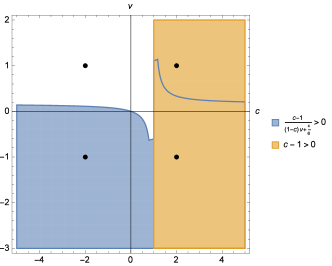
Figure 1: Region of existence of bounded $\frac{c-1}{(1-c)\nu+\frac{c}{6}}>0$, and unbounded $\frac{c-1}{(1-c)\nu+\frac{c}{6}}<0$. The solutions are bright ($c>1$), and dark ($c<1$). The 4 dots represent the values for which the solitons and periodic solutions are depicted in Fig. 2.

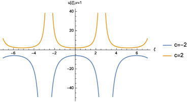
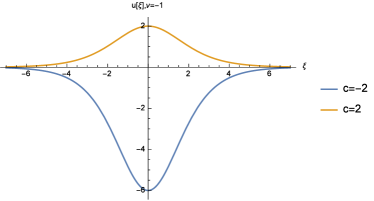
Figure 2: Unbounded (trigonometric) solutions with $\nu=1$ (left panel). Bounded solitons (hyperbolic) bright ($c=2$) and dark solitons ($c=-2$) for $\nu=-1$ (right panel) with zero B.C. given by (IV.3) for third-order KdV–BBM Eq. (III.1).

IV.1.2 Solutions in terms of elliptic functions (Nonzero B.C.)

For nonzero boundary conditions then $\mathcal{A}_{0}\neq 0,\,\mathcal{A}_{1}\neq 0$, and we use the full system (III.7) to calculate the Weierstrass invariants using (III.13)

$$\begin{array}[]{l}g_{2}=\frac{{a_{2}}^{2}-3a_{1}a_{3}}{12}=\frac{3{\mathcal{A}}_{1}+(-1+c)^{2}}{12{\mu_{1}}^{2}}\\ g_{3}=\frac{9a_{1}a_{2}a_{3}-27a_{0}{a_{3}}^{2}-2{a_{2}}^{3}}{432}=-\frac{27{\mathcal{A}}_{0}+4(-1+c)\left[9{\mathcal{A}}_{1}+2(-1+c)^{2}\right]}{1278{\mu_{1}}^{3}}.\end{array}$$ (IV.4)

Then, using the transformation (III.12), with constants from system (III.7), and germs given by (IV.4) the Weierstrass solution to the third-order KdV–BBM Eq. (III.1) is

$$u(\xi)=\frac{2}{3}(-1+c)-8\left[(1-c)\nu+\frac{c}{6}\right]\wp\left[\xi;\frac{3{\mathcal{A}}_{1}+(-1+c)^{2}}{12\left[(1-c)\nu+\frac{c}{6}\right]^{2}},-\frac{27{\mathcal{A}}_{0}+4(-1+c)[9{\mathcal{A}}_{1}+2(-1+c)^{2}]}{1278\left[(1-c)\nu+\frac{c}{6}\right]^{3}}\right].$$ (IV.5)

In Fig. 3 we present the Weierstrass solutions for nonzero boundary conditions $\mathcal{A}_{0}=1,\mathcal{A}_{1}=1$ and coefficients $\nu=\pm 1$.

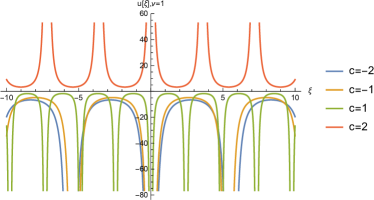
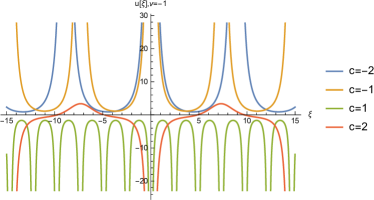
Figure 3: Weierstrass $\wp$ solutions for nozero B.C. $\mathcal{A}_{0}=1,\mathcal{A}_{1}=1$, $\nu=1$ (left panel), and $\nu=-1$ (right panel) given by (IV.5) for third-order KdV–BBM Eq. (III.1).

IV.2 Fifth order equation

IV.2.1 Solutions in terms of elementary functions (Zero B.C.)

Proceeding is a similar manner, the system (III.10) with $a_{0}=a_{1}=0\Rightarrow\mathcal{B}_{1}=0$ gives

$$\begin{array}[]{l}\frac{15}{2}\mu_{2}{a_{3}}^{2}+(5\gamma-\frac{1}{12})a_{3}=\frac{1}{4}\\ \frac{15}{2}\mu_{2}a_{2}a_{3}+(4\gamma-\frac{1}{12})a_{2}+\frac{c}{4}a_{3}=-\frac{3}{4}\\ \mu_{2}{a_{2}}^{2}+\frac{c}{6}a_{2}=c-1.\\ \end{array}$$ (IV.6)

By finding $a_{2}$ from the last equation and $a_{3}$ from the first we obtain

$$\begin{array}[]{l}a_{2}=\frac{-c\pm\sqrt{c^{2}+144\mu_{2}(c-1)}}{12\mu_{2}},\\ a_{3}=\frac{1-60\gamma\pm\sqrt{(1-60\gamma)^{2}+1080\mu_{2}}}{180\mu_{2}}.\\ \end{array}$$ (IV.7)

For real solutions the constants $c,\mu_{2},\gamma$ must be chosen such that

$$(1-60\gamma)^{2}+1080\mu_{2}\geq 0\,\wedge\,c^{2}+144\mu_{2}(c-1)\geq 0,$$

together with the level curves

$$h(\mu_{2},c)=\frac{15}{2}\mu_{2}a_{2}a_{3}+\left(4\gamma-\frac{1}{12}\right)a_{2}+\frac{c}{4}a_{3}+\frac{3}{4}=0.$$ (IV.8)

Thus, the solution of

$${u_{\xi}}^{2}=\frac{-c\pm\sqrt{c^{2}+144\mu_{2}(c-1)}}{12\mu_{2}}u^{2}+\frac{1-60\gamma\pm\sqrt{(1-60\gamma)^{2}+1080\mu_{2}}}{180\mu_{2}}u^{3}$$ (IV.9)

is given by

$$u(\xi)=\frac{15\left(-c\pm\sqrt{c^{2}+144\mu_{2}(-1+c)}\right)}{60\gamma-1\pm\sqrt{(1-60\gamma)^{2}+1080\mu_{2}}}\mathrm{sech}^{2}\left[\frac{\sqrt{3}\xi}{12}\sqrt{\frac{-c\pm\sqrt{c^{2}+144\mu_{2}(-1+c)}}{\mu_{2}}}\right].$$ (IV.10)

For the non Hamiltonian case, $\gamma\neq\frac{1}{12}$, we choose $\gamma=\frac{1}{6}$, and varying $c$, we obtain unbounded solutions as well as both dark and bright solitons, which are presented in Fig. 4.

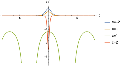
Figure 4: Evolution of bright ($c=-2,-1$) and dark solitons ($c=2$), together with unbounded periodic functions ($c=1$) with zero B.C. given by solution (IV.10) for the fifth-order KdV–BBM Eq. (III.2), and $\gamma=\frac{1}{6}$.

For the Hamiltonian case, $\gamma=\frac{1}{12}$, we obtain $a_{2}=\frac{-c\pm\sqrt{c^{2}+144\mu_{2}(c-1)}}{12\mu_{2}}$ and $a_{3}=\frac{-2\pm\sqrt{4+270\mu_{2}}}{90\mu_{2}}$. For real solutions the constants $c,\mu_{2}$ must be chosen such that $4+270\mu_{2}\geq 0\,\wedge\,c^{2}+144\mu_{2}(c-1)\geq 0$ which in turn gives either $\mu_{2}\in[-\frac{2}{135},0)$ or $\mu_{2}>0\wedge c\in(-\infty,-72\mu_{2}-12\sqrt{\mu_{2}+36\mu_{2}^{2}})\cup(-72\mu_{2}+12\sqrt{\mu_{2}+36\mu_{2}^{2}},\infty)$. Bounded solitons which are presented in Fig. 5.

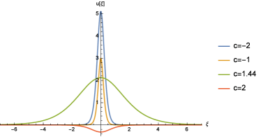
Figure 5: Evolution of bright ($c=-2,-1,1.44$) and dark ($c=2$) solitary waves with zero B.C. given by solution (IV.10) for the fifth-order KdV–BBM Eq. (III.2), and $\gamma=\frac{1}{12}.$

IV.2.2 Solutions in terms of elliptic functions (Nonzero B.C.)

Finally, we use all four equations of system (III.10) and we choose $\mathcal{B}_{1}=1$, $\gamma=\frac{1}{12}$, and constants $\delta_{2},\delta_{1}$ such that $\mu_{2}=1$ to obtain the coefficients

$$\begin{array}[]{l}a_{0}=\frac{180(1389041+848558\sqrt{274})+c\{95933536+87674598\sqrt{274}+c[-364106754+668133\sqrt{274}+c(19508\sqrt{274}-1623565)]\}}{2475480735},\\ a_{1}=\frac{c[-4086+9117\sqrt{274}+c(41\sqrt{274}-145)]-360(33\sqrt{274}-59)}{124215},\\ a_{2}=\frac{c(\sqrt{274}-92)-90(\sqrt{274}-1)}{2730},\\ a_{3}=\frac{\sqrt{274}-2}{90}.\end{array}$$ (IV.11)

We also find the germs using system (IV.4) to obtain the expressions

$$\begin{array}[]{l}g_{2}=\frac{c[-56426+682\sqrt{274}+3c(\sqrt{274}-53)]+98030-1180\sqrt{274}}{993720},\\ g_{3}=\frac{-80610056+1243238\sqrt{274}+c\{94841830-23958914\sqrt{274}+c[16001978-222019\sqrt{274}+c(91838-2125\sqrt{274})]\}}{101848350240}.\end{array}$$ (IV.12)

Thus, the solution of the fifth-order KdV–BBM Eq. (III.2) is obtained using the transformation (III.12) with coefficients from system (IV.11), and germs given by (IV.12). The Weierstrass solutions are presented in Fig. 6 and are shown for $\gamma=\frac{1}{12}$ and $\mu_{2}=1$.

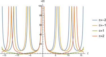
Figure 6: Weierstrass $\wp$ solutions with nonzero B.C. and $\gamma=\frac{1}{12},\mu_{2}=1$ for the fifth-order KdV–BBM Eq. (III.2).

V Conclusion

We have provided conditions for parameters for both third and fifth-order KdV–BBM regularized long wave equations that yield hyperbolic, trigonometric and elliptic solutions in terms of Weierstrass $\wp$ functions.

For the third-order KdV–BBM equation an analysis for the initial value problem has been developed together with a local well-posedness theory in relatively weak solution spaces. The global well-posedness is settled in the case of $\nu<\frac{1}{6}$. For zero boundary conditions, and using a traveling wave ansatz we obtained periodic (trigonometric) and solitary (hyperbolic) waves which are both bright or dark with no restrictions on the parameter $\nu$ or the velocity $c$. For nonzero boundary conditions we showed a procedure using a balancing principle on how to construct solutions in terms of Weierstrass $\wp$ functions.

For the fifth-order KdV–BBM equation, motivated by the seemingly lack of a Hamiltonian structure for $\gamma\neq\frac{1}{12}$ we focused on the intrinsic properties of traveling wave solutions only. We developed $H^{k}$ bounds for these solutions under the assumption that they are not bounded. We found that in the traveling wave variable $\xi$, $\gamma=\frac{1}{12}$ represents a restriction for which none of the constraint curves intersect the region of unbounded solitary waves, which shows that only dark or bright solitons and no unbounded solutions exist. When $\gamma\neq\frac{1}{12}$ since there is no restriction and the system is not Hamiltonian, solitons that are bright and dark coexist together with unbounded periodic solutions. For nonzero boundary conditions, due to the complexity of the nonlinear algebraic system of the coefficients of the elliptic equation, we have shown how Weierstrass solutions can also be constructed for a particular set of parameters.

References

References

- (1) X. Carvajal, M. Panthee, M. Scialom, Comparison between model equations for long waves and blow-up phenomena, Journal of Mathematical Analysis and Applications 442 (1) (2016) 273–290.
- (2) J. L. Bona, X. Carvaxal, M. Panthee, M. Scialom, Higher-order Hamiltonian model for unidirectional water waves, arXiv preprint:1509.08510.
- (3) A. A. Alazman, J. P. Albert, J. L. Bona, M. Chen, J. Wu, Comparisons between the BBM equation and a Boussinesq system, Advances in Differential Equations 11 (2006) 121–166.
- (4) J. L. Bona, T. Colin, D. Lannes, Long wave approximations for water waves, Archive for Rational Mechanics and Analysis 178 (2005) 373–410.
- (5) J. L. Bona, W. G. Pritchard, L. R. Scott, An evaluation of a model equation for water waves, Philosophical Transactions of the Royal Society London Series A 302 (1981) 457–510.
- (6) J. L. Bona, W. G. Pritchard, L. R. Scott, A comparison of solutions of two model equations for long waves, in: N. Lebovitz (Ed.), ADA128076, Vol. 20 of Lectures in Applied Mathematics, American Mathematical Society: Providence, 1983, pp. 235–267.
- (7) J. L. Hammack, A note on tsunamis, their generation and propagation in an ocean of uniform depth, Journal of Fluid Mechanics 60 (1973) 769–799.
- (8) J. L. Hammack, H. Segur, The Korteweg-de Vries equation and water waves. Part 2. Comparison with experiments, Journal of Fluid Mechanics 65 (1974) 289–314.
- (9) J. L. Bona, M. Chen, Higher-order Boussinesq systems for two-way propagation of water waves, in: L. Ta-Tsien (Ed.), Proceedings of the Conferences on Nonlinear Evolution Equations and Infinite-Dimensional Dynamical Systems, Vol. 1 of 12-16 June 1995, Shanghai, China, World Scientific Publishing Co.: Singapore, 1997, pp. 5–12.
- (10) J. L. Bona, M. Chen, J.-C. Saut, Boussinesq equations and other systems for small- amplitude long waves in nonlinear dispersive media I. Derivation and linear theory, Journal of Nonlinear Science 12 (2002) 283–318.
- (11) J. L. Bona, M. Chen, J.-C. Saut, Boussinesq equations and other systems for small-amplitude long waves in nonlinear dispersive media II. The nonlinear theory, Nonlinearity 17 (2004) 925–952.
- (12) J. Boussinesq, Essai sur la théorie des eaux courantes, Imprimerie nationale, 1877.
- (13) R. Fetecau, D. Levy, Approximate model equations for water waves, Communications in Mathematical Sciences 3 (2005) 159–170.
- (14) M. Chen, O. Goubet, Long -time asymptotic behavior of dissipative Boussinesq systems, Dynamical Systems 17 (2007) 509–528.
- (15) D. Lannes, The water waves problem: mathematical analysis and asymptotics, American Mathematical Society, 2013.
- (16) D. Ambrose, J. Bona, D. Nicholls, On ill-posedness of truncated series models for water waves, in: Proceedings of the Royal Society of London A, no. 2166 in 470, The Royal Society, 2014, p. 20130849.
- (17) D. Ambrose, J. Bona, D. Nicholls, Well-posedness of a model for water waves with viscosity, Discrete and Continuous Dynamical Systems Series B 17 (2012) 1113–1137.
- (18) Y. Kodama, Normal forms for weakly dispersive wave equations, Physics Letters A 112 (1985) 193–196.
- (19) Y. Hiraoka, Y. Kodama, Normal form and solitons, in: Integrability, Springer, 2009, pp. 175–214.
- (20) A. Fokas, Q. Liu, Asymptotic integrability of water waves, Physical Review Letters 77 (1996) 2347.
- (21) C. Cosgrove, Chazy Classes IX–XI Of Third-Order Differential Equations, Studies in Applied Mathematics 104 (2000) 171–228.
- (22) R. Grimshaw, E. Pelinovsky, T. Talipova, Modelling internal solitary waves in the coastal ocean, Surveys in Geophysics 28 (2007) 273–298.
- (23) D. Dutykh, T. Katsaounis, D. Mitsotakis, Finite volume methods for unidirectional dispersive wave models, International Journal for Numerical Methods in Fluids 71 (2013) 717–736.
- (24) S. C. Mancas, G. Spradlin, H. Khanal, Weierstrass traveling wave solutions for dissipative Benjamin, Bona, and Mahony (BBM) equation, Journal of Mathematical Physics 54 (2013) 081502.
- (25) J. Nickel, Elliptic solutions to a generalized BBM equation, Physics Letters A 364 (2007) 221–226.
- (26) N. Kudryashov, Painlevé analysis and exact solutions of the Korteweg–de Vries equation with a source, Applied Mathematics Letters 41 (2015) 41–45.
- (27) J. L. Bona, H. Kalisch, Models for internal waves in deep water, Discrete and Continuous Dynamical Systems 6 (2000) 1–20.
- (28) J. L. Bona, R. Scott, The Korteweg-de Vries equation in fractional order Sobolev spaces, Duke Mathematical Journal 43 (1976) 87–99.
- (29) J. L. Bona, J. Cohen, G. Wang, Global well-posedness for a system of KdV-type equations with coupled quadratic nonlinearities, Nagoya Mathematical Journal 215 (2014) 67–149.
- (30) H. Chen, M. Chen, N. Nguyen, Cnoidal wave solutions to boussinesq systems, Nonlinearity 20 (2007) 1443.
- (31) P. Razborova, B. Ahmed, A. Biswas, Solitons, shock waves and conservation laws of Rosenau-KdV-RLW equation with power law nonlinearity, Applied Mathematics & Information Sciences 8 (2014) 485–491.
- (32) J. M. Zuo, Solitons and periodic solutions for the Rosenau–KdV and Rosenau–Kawahara equations, Applied Mathematics and Computation 215 (2009) 835–840.
- (33) A. Esfahani, R. Pourgholi, Dynamics of solitary waves of the Rosenau-RLW equation, Differential Equations and Dynamical Systems 22 (2014) 93–111.
- (34) M. Abramowitz, I. Stegun, Handbook of mathematical functions: with formulas, graphs, and mathematical tables, Courier Corporation, 1964.