Alternating Direction Method of Multipliers
for Linear Inverse Problems

Abstract

In this paper we propose an iterative method using alternating direction method of multipliers (ADMM) strategy to solve linear inverse problems in Hilbert spaces with general convex penalty term. When the data is given exactly, we give a convergence analysis of our ADMM algorithm without assuming the existence of Lagrange multiplier. In case the data contains noise, we show that our method is a regularization method as long as it is terminated by a suitable stopping rule. Various numerical simulations are performed to test the efficiency of the method.

1 Introduction

The study of linear inverse problems gives rise to the linear equation of the form

$$Ax=b,$$ (1)

where $A:\mathcal{X}\to\mathcal{H}$ is a bounded linear operator between two Hilbert spaces $\mathcal{X}$ and $\mathcal{H}$. In applications, we will not simply consider (1) alone, instead we will incorporate a priori available information on solutions into the problem. Assume that we have a priori information on the feature, such as sparsity, of the sought solution under a suitable transform $W$ from $\mathcal{X}$ to another Hilbert spaces $\mathcal{Y}$ with domain $\mathscr{D}(W)$. We may then take a convex function $f:\mathcal{Y}\to(-\infty,\infty]$ to capture such feature. This leads us to consider the convex minimization problem

$$\left\{\begin{array}[]{lll}\mbox{minimize }&f(Wx)\\ \mbox{subject to }&Ax=b,\ \ \ x\in\mathscr{D}(W),\end{array}\right.$$ (4)

where $f$ and $W$ should be specified during applications. For inverse problems, the operator $A$ usually is either non-invertible or ill-conditioned with a huge condition number. Thus, a small perturbation of the data may lead the problem (4) to have no solution; even if it has a solution, this solution may not depend continuously on the data due to the uncontrollable amplification of noise. In order to overcome such ill-posedness, regularization techniques should be taken into account to produce a reasonable approximate solution from noisy data. One may refer to [17, 30, 45] for comprehensive accounts on the variational regularization methods as well as iterative regularization methods.

Variational regularization methods typically consider (4) by solving a family of well-posed minimization problems

$$\min_{x\in\mathscr{D}(W)}\left\{\frac{1}{2}\|Ax-b\|^{2}+\alpha f(Wx)\right\},$$ (5)

where $\alpha>0$ is the so called regularization parameter whose choice crucially affects the performance of the method. When the regularization parameter $\alpha$ is given, many efficient solvers have been developed to solve (5) when $f$ are sparsity promoting functions. However, to find a good approximate solution, the regularization parameter $\alpha$ should be carefully chosen, consequently one has to solve (5) for many different values of $\alpha$, which can be time-consuming.

Among algorithms for solving (5), the alternating direction method of multipliers (ADMM) is a favorable one. The ADMM was proposed in [22, 24] around the mid-1970 and was analyzed in [16, 21, 36, 43]. It has been widely used in solving structured optimization problems due to its decomposability and superior flexibility. Recently, it has been revisited and popularized in modern signal/image processing, statistics, machine learning, and so on; see the recent survey paper [4] and the references therein. Due to the popularity of ADMM and its variants, new and refined convergence results have been obtained from several different perspectives, see, for example, [9, 12, 13, 25, 26, 27, 29, 35, 48], just to name a few of them. To the best of our knowledge, the existing convergence analyses of ADMM depend on the solvability of the dual problem or the existence of saddle points for the corresponding Lagrangian function, which might not be true for inverse problems (4).

In this paper we propose an ADMM algorithm in the framework of iterative regularization methods. By introducing an additional variable $y=Wx$, we can reformulate (4) into the equivalent form

$$\left\{\begin{array}[]{lll}\mbox{minimize }&f(y)\\ \mbox{subject to }&Ax=b,\ \ \ Wx=y,\,\,\,x\in\mathscr{D}(W).\end{array}\right.$$ (8)

The corresponding augmented Lagrangian function is

$$L_{\rho_{1},\rho_{2}}(x,y;\lambda,\mu) =f(y)+\langle\lambda,Ax-b\rangle+\langle\mu,Wx-y\rangle$$

$$\quad\,+\frac{\rho_{1}}{2}\|Ax-b\|^{2}+\frac{\rho_{2}}{2}\|Wx-y\|^{2},$$ (9)

where $\rho_{1}$ and $\rho_{2}$ are two positive constants. Our ADMM algorithm then reads

$$\left\{\begin{array}[]{l}x_{k+1}=\arg\min_{x\in\mathscr{D}(W)}\;L_{\rho_{1},\rho_{2}}(x,y_{k};\lambda_{k},\mu_{k}),\\[5.16663pt] y_{k+1}=\arg\min_{y\in\mathcal{Y}}\;L_{\rho_{1},\rho_{2}}(x_{k+1},y;\lambda_{k},\mu_{k}),\\[5.16663pt] \lambda_{k+1}=\lambda_{k}+\rho_{1}(Ax_{k+1}-b),\\[5.16663pt] \mu_{k+1}=\mu_{k}+\rho_{2}(Wx_{k+1}-y_{k+1}).\end{array}\right.$$ (10)

The $x$-subproblem in (10) is a quadratical minimization problem, which can be solved by many methods, and the $y$-subproblem can be solved explicitly when $f$ is properly chosen, e.g., $f$ are certain sparsity promoting functions, Thus, our ADMM algorithm can be efficiently implemented. When the data $b$ in (4) is consistent in the sense that $b=Ax$ for some $x\in\mathscr{D}(W)$ with $Wx\in\mathscr{D}(f)$, and when $f$ is strongly convex, we give a convergence analysis of our ADMM algorithm by using tools from convex analysis. The proof is based on several remarkable monotonicity results and does not need the existence of the Lagrange multiplier to (8). When the data contains noise, similar as other iterative regularization methods, our ADMM algorithm shows the semi-convergence property, i.e. the iterate becomes close to the sought solution at the beginning, however, after a critical number of iterations, the iterate leaves the sought solution far away as the iteration proceeds. By proposing a suitable stopping rule, we establish the regularization property of our algorithm. To the best of our knowledge, this is the first time that ADMM is used to solve inverse problems directly as an iterative regularization method.

There are several different iterative regularization methods proposed for solving (4). The augmented Lagrangian method (ALM) is a popular and efficient algorithm which takes the form

$$\left\{\begin{array}[]{l}x_{k+1}=\arg\min_{x\in\mathscr{D}(W)}\left\{f(Wx)+\langle\lambda_{k},Ax-b\rangle+\frac{\rho_{k}}{2}\|Ax-b\|^{2}\right\},\\[6.02773pt] \lambda_{k+1}=\lambda_{k}+\rho_{k}(Ax_{k+1}-b),\end{array}\right.$$ (11)

where $\{\rho_{k}\}$ is a sequence of positive numbers satisfying suitable properties. ALM was originally proposed by Hestenes [28] and Powell [41] independently; see [2, 42] for its convergence analysis for well-posed optimization problems. Recently, ALM has been applied to solve ill-posed inverse problems in [18, 19, 20, 34, 40]. It has been shown that ALM can produce a satisfactory approximate solution within a few iterations if $\{\rho_{k}\}$ is chosen to be geometrically increasing. However, since $f(Wx)$ and $A$ are coupled, solving the $x$-subproblem in (11) is highly nontrivial, and an additional inner solver should be incorporated into the algorithm. To remedy this drawback, a linearization step can be introduced to modify the $x$-subproblem in (11) which leads to the Uzawa-type iteration

$$\left\{\begin{array}[]{l}\lambda_{k+1}=\lambda_{k}+\rho_{k}(Ax_{k}-b),\\[4.30554pt] x_{k+1}=\arg\min_{x\in\mathscr{D}(W)}\left\{f(Wx)+\langle\lambda_{k+1},Ax-b\rangle\right\}.\end{array}\right.$$ (12)

This method and its variants have been analyzed in [3, 31, 32] for ill-posed inverse problems. Unlike (11), the resolution of the $x$-subproblem in (12) only relies on $f(Wx)$ and hence is much easier for implementation. For instance, if the sought solution is sparse, one may take $f(x)=\|x\|_{\ell^{1}}+\frac{\nu}{2}\|x\|^{2}$ and $W=I$ the identity, then the $x$-subproblem in (12) can be solved explicitly by the soft thresholding. However, if the sought solution is sparse under a transform $W$ that is not identity, which can occur when using the total variation [44], the wavelet frame [15, 46], and so on, the $x$-subproblem in (12) does not have a closed form solution and an inner solver is needed. In contrast to (11) and (12), our ADMM algorithm (10) can admit closed form solutions for each subproblem for many important applications.

The rest of this paper is organized as follows. In Section 2, we give conditions to guarantee that (4) has a unique solution, show that our ADMM (10) is well-defined and establish an important monotonicity result. When the data is given exactly, we provide various convergence results of (10). When the data contains noise, we propose a stopping rule to terminate the iteration and show that our ADMM renders into a regularization method. In Section 3 we report various numerical results to test the efficiency of our ADMM algorithm. Finally, we draw conclusions in Section 4.

2 The method and its convergence analysis

2.1 Preliminary

We consider the convex minimization problem (4) arising from linear inverse problems, where $A:\mathcal{X}\to\mathcal{H}$ is a bounded linear operator between two Hilbert spaces $\mathcal{X}$ and $\mathcal{H}$, $W$ is a linear operator from $\mathcal{X}$ to another Hilbert spaces $\mathcal{Y}$ with domain $\mathscr{D}(W)$, and $f:\mathcal{Y}\to(-\infty,\infty]$ is a convex function. The inner products and norms on $\mathcal{X}$, $\mathcal{Y}$ and $\mathcal{H}$ will be simply denoted by $\langle\cdot,\cdot\rangle$ and $\|\cdot\|$ respectively, which should be clear from the context. Throughout the paper we will make the following assumptions on the operators $W$, $A$ and the function $f$:

• $A:\mathcal{X}\to\mathcal{H}$ is a bounded linear operator. We use $A^{*}:\mathcal{H}\to\mathcal{X}$ to denote its adjoint.

• $f:\mathcal{Y}\to(-\infty,\infty]$ is a proper, lower semi-continuous, strongly convex function in the sense that there is a constant $c_{0}>0$ such that

  $$f(ty_{1}+(1-t)y_{2})+c_{0}t(1-t)\|y_{1}-y_{2}\|^{2}\leq tf(y_{1})+(1-t)f(y_{2})$$ (13)

  for all $y_{1},y_{2}\in\mathcal{Y}$ and $0\leq t\leq 1$.

• $W:\mathcal{X}\to\mathcal{Y}$ is a densely defined, closed, linear operator with domain $\mathscr{D}(W)$.

• There is a constant $c_{1}>0$ such that

  $$\|Ax\|^{2}+\|Wx\|^{2}\geq c_{1}\|x\|^{2},\qquad\forall x\in\mathscr{D}(W).$$

The assumptions (A1) and (A2) are standard. We will use $\partial f(y)$ to denote the subdifferential of $f$ at $y$, i.e.

$$\partial f(y)=\{\mu\in\mathcal{Y}:f(\bar{y})\geq f(y)+\langle\mu,\bar{y}-y\rangle\mbox{ for all }\bar{y}\in\mathcal{Y}\}.$$

Let $\mathscr{D}(\partial f)=\{y\in\mathcal{Y}:\partial f(y)\neq\emptyset\}$. Then for $y\in\mathscr{D}(\partial f)$ and $\mu\in\partial f(y)$ we can introduce

$$D_{\mu}f(\bar{y},y)=f(\bar{y})-f(y)-\langle\mu,\bar{y}-y\rangle,\quad\forall\bar{y}\in\mathcal{Y}$$

which is called the Bregman distance induced by $f$ at $y$ in the direction $\mu$, see [5]. When $f$ is strongly convex in the sense of (13), by definition one can show that

$$D_{\mu}f(\bar{y},y)\geq c_{0}\|\bar{y}-y\|^{2}$$ (14)

for all $\bar{y}\in\mathcal{Y}$, $y\in\mathscr{D}(\partial f)$ and $\mu\in\partial f(y)$. Moreover

$$\langle\mu-\bar{\mu},y-\bar{y}\rangle\geq 2c_{0}\|y-\bar{y}\|^{2}$$ (15)

for all $y,\bar{y}\in\mathscr{D}(\partial f)$, $\mu\in\partial f(y)$ and $\bar{\mu}\in\partial f(\bar{y})$.

The assumptions (A3) and (A4) are standard conditions used in the literature on regularization methods with differential operators, see [17, 37, 38], they will be used to show that our ADMM (10) is well-defined. The closedness of $W$ in (A3) implies that $W$ is also weakly closed. We can define the adjoint $W^{*}$ of $W$ which is also closed and densely defined. Moreover, $z\in\mathscr{D}(W^{*})$ if and only if $\langle W^{*}z,x\rangle=\langle z,Wx\rangle$ for all $x\in\mathscr{D}(W)$. A sufficient condition which guarantees (A4) is that

$$W\mbox{ has a closed range in }\mathcal{Y},\quad\dim\textrm{Ker}\;W<+\infty,\quad\textrm{Ker}\;W\cap\textrm{Ker}\;A=\{0\};$$ (16)

see [17, Chapter 8]. This sufficient condition is important in practice as it is satisfied by many interesting examples. For instance, consider the following three examples:

• $W=I$ the identity operator with $\mathscr{D}(W)=\mathcal{X}=\mathcal{Y}$.

• $W$ is a frame transform, i.e., there exist $0<c\leq C<+\infty$ such that

  $$c\|\varphi\|^{2}\leq\|W\varphi\|^{2}\leq C\|\varphi\|^{2},\quad\forall\varphi\in\mathcal{X}$$

  with $\mathscr{D}(W)=\mathcal{X}=L^{2}(\Omega)$ and $\mathcal{Y}=\ell^{2}(\mathbb{N})$.

• The constant function 1 is not in the kernel of $A$, $W=\nabla$ the gradient operator with $\mathcal{X}=L^{2}(\Omega)$, $\mathscr{D}(W)=H^{1}(\Omega)$ and $\mathcal{Y}=[L^{2}(\Omega)]^{d}$.

For (i), the conditions (A3) and (16) hold trivially. For (ii), (A3) follows from [10, Proposition 12.7] and (16) follows from the coercivity of $W$ (see e.g. [10, pp. 107]). For (iii), when $\Omega\subset{\mathbb{R}}^{d}$ with $d\leq 3$ is an open bounded domain with Lipschitz boundary, (A3) follows from the definition of weak derivatives. Note that $\textrm{Ker}\;W$ is a one dimension subspace. This fact together with the Helmholtz-Hodge decomposition (see [23, Theorem 3.4]) implies (16).

Under the assumptions (A1)–(A4), the following result shows that the minimization problem (4) admits a unique solution whenever $b$ is consistent in the sense that $b=Ax$ for some $x\in\mathscr{D}(W)$ with $Wx\in\mathscr{D}(f)$.

Theorem 1.

Let $b$ in (4) be consistent and let (A1)–(A4) hold. Then the optimization problem (4) admits a unique solution $x^{*}\in\mathscr{D}(W)$ with $Wx^{*}\in\mathscr{D}(f)$.

Proof.

Let $f_{*}:=\inf\{f(Wz):Az=b,\,z\in\mathscr{D}(W)\}$. Since $b$ is consistent, we have $f_{*}<\infty$. Let $\{z_{k}\}$ be the minimizing sequence such that

$$z_{k}\in\mathscr{D}(W),\quad Az_{k}=b\quad\mbox{and}\quad\lim_{k\rightarrow\infty}f(Wz_{k})=f_{*}.$$

By (A2), $f$ is strongly convex and hence is coercive, see e.g. [1, Proposition 11.16]. Thus $\{Wz_{k}\}$ is bounded in $\mathcal{Y}$. In view of (A4), $\{z_{k}\}$ is bounded in $\mathcal{X}$. Therefore, $\{z_{k}\}$ has a subsequence, which is denoted by the same notation, such that

$$z_{k}\rightarrow x^{*}\textrm{ weakly in }\mathcal{X},\quad Wz_{k}\rightarrow y^{*}\textrm{ weakly in }\mathcal{Y}.$$

By using (A3) and $\{z_{k}\}\subset\mathscr{D}(W)$, we have $x^{*}\in\mathscr{D}(W)$ and $y^{*}=Wx^{*}$. Since $f$ is convex and lower semi-continuous, $f$ is also weakly lower semi-continuous (see [1, Proposition 10.23]). Thus $f(Wx^{*})\leq\liminf_{k\rightarrow\infty}f(Wz_{k})=f_{*}$ and hence $x^{*}$ is an optimal solution of (4). The uniqueness follows by the strong convexity of $f$ and (A4). ∎

2.2 ADMM algorithm and basic estimates

As described in the introduction, by introducing an additional variable $y=Wx$, we can reformulate (4) into the equivalent form (8). Recall the augmented Lagrangian function (1), our ADMM (10) starts from some initial guess $y_{0}\in\mathcal{Y}$, $\lambda_{0}\in\mathcal{H}$, $\mu_{0}\in\mathcal{Y}$ and defines

$$x_{k+1} =\arg\min_{x\in\mathscr{D}(W)}\left\{\langle\lambda_{k},Ax\rangle+\langle\mu_{k},Wx\rangle+\frac{\rho_{1}}{2}\|Ax-b\|^{2}+\frac{\rho_{2}}{2}\|Wx-y_{k}\|^{2}\right\},$$ (17)

$$y_{k+1} =\arg\min_{y\in\mathcal{Y}}\left\{f(y)-\langle\mu_{k},y\rangle+\frac{\rho_{2}}{2}\|Wx_{k+1}-y\|^{2}\right\},$$ (18)

$$\lambda_{k+1} =\lambda_{k}+\rho_{1}(Ax_{k+1}-b),$$ (19)

$$\mu_{k+1} =\mu_{k}+\rho_{2}(Wx_{k+1}-y_{k+1})$$ (20)

for $k=0,1,\cdots$, where $\rho_{1}$ and $\rho_{2}$ are two fixed positive constants.

We need to show that $x_{k+1}$ and $y_{k+1}$ are well-defined. Note that (17) and (18) can be written as

$$x_{k+1} =\arg\min_{x\in\mathscr{D}(W)}\left\{\frac{\rho_{1}}{2}\|Ax-b+\lambda_{k}/\rho_{1}\|^{2}+\frac{\rho_{2}}{2}\|Wx-y_{k}+\mu_{k}/\rho_{2}\|^{2}\right\},$$

$$y_{k+1} =\arg\min_{y\in\mathcal{Y}}\left\{f(y)+\frac{\rho_{2}}{2}\|y-Wx_{k+1}-\mu_{k}/\rho_{2}\|^{2}\right\}.$$

Therefore, the well-posedness of $x_{k+1}$ and $y_{k+1}$ follows from the following result.

Lemma 2.

Let Assumptions (A1)–(A4) hold.

• For any $h\in\mathcal{H}$ and $v\in\mathcal{Y}$, the minimization problem

  $$\min_{z\in\mathscr{D}(W)}\left\{\frac{\rho_{1}}{2}\|Az-h\|^{2}+\frac{\rho_{2}}{2}\|Wz-v\|^{2}\right\}$$ (21)

  admits a unique solution $z$. Moreover, $z$ and $Wz$ depend continuously on $h$ and $v$.

• For any $v\in\mathcal{Y}$ the minimization problem

  $$\min_{y\in\mathcal{Y}}\left\{f(y)+\frac{\rho_{2}}{2}\|y-v\|^{2}\right\}$$ (22)

  admits a unique solution $y$. Moreover, $y$ and $f(y)$ depend continuously on $v$.

Proof.

(i) follows from [39, pp. 23 Theorem 4 and pp. 26 Theorem 6] and (ii) follows from [33, Lemma 2.2]. ∎

We now take a closer look at the ADMM algorithm (17)–(20). From (17) it follows that $x_{k+1}\in\mathscr{D}(W)$ satisfies the optimality condition

$$\langle A^{*}\lambda_{k}+\rho_{1}A^{*}(Ax_{k+1}-b),x\rangle+\langle\mu_{k}+\rho_{2}(Wx_{k+1}-y_{k}),Wx\rangle=0,\quad x\in\mathscr{D}(W).$$

This implies that $\mu_{k}+\rho_{2}(Wx_{k+1}-y_{k})\in\mathscr{D}(W^{*})$ and

$$A^{*}\lambda_{k}+\rho_{1}A^{*}(Ax_{k+1}-b)+W^{*}[\mu_{k}+\rho_{2}(Wx_{k+1}-y_{k})]=0.$$ (23)

From (18) we can obtain that

$$0\in\partial f(y_{k+1})-\mu_{k}-\rho_{2}(Wx_{k+1}-y_{k+1}).$$ (24)

For simplicity of exposition, we introduce the residuals

$$r_{k}=Ax_{k}-b\quad\mbox{and}\quad s_{k}=Wx_{k}-y_{k},\quad k=1,2,\cdots.$$

It then follows from (19), (20), (23) and (24) that

$$\lambda_{k+1}-\lambda_{k} =\rho_{1}r_{k+1},$$ (25)

$$\mu_{k+1}-\mu_{k} =\rho_{2}s_{k+1},$$ (26)

$$\mu_{k+1} \in\partial f(y_{k+1}),$$ (27)

$$A^{*}\lambda_{k}+\rho_{1}A^{*}r_{k+1} =-W^{*}[\mu_{k}+\rho_{2}(Wx_{k+1}-y_{k})]$$ (28)

for $k=0,1,\cdots$.

Lemma 3.

There holds $A^{*}\lambda_{1}=W^{*}[\rho_{2}(y_{0}-y_{1})-\mu_{1}]$. Moreover, for $k\geq 1$ there holds $\rho_{1}A^{*}r_{k+1}=\rho_{2}W^{*}[(y_{k}-y_{k+1})-(y_{k-1}-y_{k})-s_{k+1}],$ that is

$$\rho_{1}\langle r_{k+1},Ax\rangle=\rho_{2}\langle(y_{k}-y_{k+1})-(y_{k-1}-y_{k})-s_{k+1},Wx\rangle$$

for all $x\in\mathscr{D}(W)$.

Proof.

From (25) we have $A^{*}\lambda_{k+1}-A^{*}\lambda_{k}=\rho_{1}A^{*}r_{k+1}$ for $k\geq 0$. This together with (26) and (28) gives for $k\geq 0$ that

$$A^{*}\lambda_{k+1} =A^{*}\lambda_{k}+\rho_{1}A^{*}r_{k+1}+W^{*}(\rho_{2}s_{k+1}+\mu_{k}-\mu_{k+1})$$

$$=W^{*}[\rho_{2}(y_{k}-y_{k+1})-\mu_{k+1}]$$ (29)

which in particular implies $A^{*}\lambda_{1}=W^{*}[\rho_{2}(y_{0}-y_{1})-\mu_{1}]$. Further, by using (25), (2.2) and (26) we have

$$\rho_{1}A^{*}r_{k+1} =A^{*}\lambda_{k+1}-A^{*}\lambda_{k}=W^{*}\left[\rho_{2}(y_{k}-y_{k+1})-\rho_{2}(y_{k-1}-y_{k})+\mu_{k}-\mu_{k+1}\right]$$

$$=\rho_{2}W^{*}[(y_{k}-y_{k+1})-(y_{k-1}-y_{k})-s_{k+1}]$$

for $k\geq 1$, which completes the proof. ∎

The following monotonicity result plays an essential role in the forthcoming convergence analysis.

Lemma 4.

Let $E_{k}=\rho_{1}\|r_{k}\|^{2}+\rho_{2}\|s_{k}\|^{2}+\rho_{2}\|y_{k}-y_{k-1}\|^{2}$. Then

$$E_{k+1}-E_{k}\leq-\rho_{1}\|r_{k+1}-r_{k}\|^{2}-4c_{0}\|y_{k+1}-y_{k}\|^{2}$$

for all $k\geq 1$. In particular, $E_{k}$ is monotonically decreasing along the iteration and $\sum_{k=1}^{\infty}\|y_{k+1}-y_{k}\|^{2}<\infty$.

Proof.

By the definition of $r_{k}$ and $s_{k}$ we have

$$r_{k+1}-r_{k} =A(x_{k+1}-x_{k}),$$ (30)

$$s_{k+1}-s_{k} =W(x_{k+1}-x_{k})+(y_{k}-y_{k+1}).$$ (31)

Therefore

$$\rho_{1}\left\langle r_{k+1}-r_{k},r_{k+1}\right\rangle+\rho_{2}\left\langle s_{k+1}-s_{k},s_{k+1}\right\rangle$$

$$=\rho_{1}\left\langle A(x_{k+1}-x_{k}),r_{k+1}\right\rangle+\rho_{2}\left\langle W(x_{k+1}-x_{k})+(y_{k}-y_{k+1}),s_{k+1}\right\rangle.$$

Recall that $x_{k+1}-x_{k}\in\mathscr{D}(W)$. We may use Lemma 3, (26), (27) and (15) to derive that

$$\rho_{1}\langle r_{k+1}-r_{k},r_{k+1}\rangle+\rho_{2}\langle s_{k+1}-s_{k},s_{k+1}\rangle$$

$$=\rho_{2}\langle W(x_{k+1}-x_{k}),(y_{k}-y_{k+1})-(y_{k-1}-y_{k})\rangle-\langle y_{k+1}-y_{k},\mu_{k+1}-\mu_{k}\rangle$$

$$\leq\rho_{2}\langle W(x_{k+1}-x_{k}),(y_{k}-y_{k+1})-(y_{k-1}-y_{k})\rangle-2c_{0}\|y_{k+1}-y_{k}\|^{2}.$$

In view of (31) and the Cauchy-Schwarz inequality, we have

$$\rho_{1}\langle r_{k+1}-r_{k},r_{k+1}\rangle+\rho_{2}\langle s_{k+1}-s_{k},s_{k+1}\rangle$$

$$\leq\rho_{2}\langle(s_{k+1}-s_{k})+(y_{k+1}-y_{k}),(y_{k}-y_{k+1})-(y_{k-1}-y_{k})\rangle-2c_{0}\|y_{k+1}-y_{k}\|^{2},$$

$$\leq\frac{\rho_{2}}{2}\left(\|s_{k+1}-s_{k}\|^{2}-\|y_{k+1}-y_{k}\|^{2}+\|y_{k}-y_{k-1}\|^{2}\right)-2c_{0}\|y_{k+1}-y_{k}\|^{2}.$$

By virtue of the identity $2\langle a-b,a\rangle=\|a\|^{2}-\|b\|^{2}+\|a-b\|^{2}$, we therefore obtain

$$\rho_{1}\|r_{k+1}\|^{2}+\rho_{2}\|s_{k+1}\|^{2} \leq\rho_{1}\|r_{k}\|^{2}+\rho_{2}\|s_{k}\|^{2}-\rho_{1}\|r_{k+1}-r_{k}\|^{2}-\rho_{2}\|y_{k+1}-y_{k}\|^{2}$$

$$\quad\,+\rho_{2}\|y_{k}-y_{k-1}\|^{2}-4c_{0}\|y_{k+1}-y_{k}\|^{2}.$$

This shows the desired inequality. ∎

2.3 Exact data case

In this subsection we will give the convergence analysis of the ADMM algorithm (17)–(20) under the condition that the data $b$ is consistent so that (4) has a unique solution. We will always use $(\hat{x},\hat{y})$ to represent any feasible point of (8), i.e., $\hat{x}\in\mathscr{D}(W)$ and $\hat{y}\in\mathscr{D}(f)$ such that $A\hat{x}=b$ and $W\hat{x}=\hat{y}$.

Lemma 5.

The sequences $\{x_{k}\}$ and $\{y_{k}\}$ are bounded and

$$\sum_{k=1}^{\infty}\left\{D_{\mu_{k}}f(y_{k+1},y_{k})+E_{k}\right\}<\infty.$$

In particular, $Ax_{k}\rightarrow b$, $Wx_{k}-y_{k}\rightarrow 0$ and $y_{k+1}-y_{k}\rightarrow 0$ as $k\rightarrow\infty$.

Proof.

Let $(\hat{x},\hat{y})$ be any feasible point of (8). By using (26) and Lemma 3 we have

$$D_{\mu_{k+1}}f(\hat{y},y_{k+1})-D_{\mu_{k}}f(\hat{y},y_{k})+D_{\mu_{k}}f(y_{k+1},y_{k})$$

$$=\langle\mu_{k}-\mu_{k+1},\hat{y}-y_{k+1}\rangle=-\rho_{2}\langle s_{k+1},W(\hat{x}-x_{k+1})+s_{k+1}\rangle$$

$$=-\rho_{2}\|s_{k+1}\|^{2}+\rho_{2}\langle(y_{k-1}-y_{k})-(y_{k}-y_{k+1}),W(\hat{x}-x_{k+1})\rangle$$

$$\quad\,+\rho_{1}\langle r_{k+1},A(\hat{x}-x_{k+1})\rangle$$

$$=-\rho_{1}\|r_{k+1}\|^{2}-\rho_{2}\|s_{k+1}\|^{2}+\rho_{2}\langle y_{k-1}-y_{k},W(\hat{x}-x_{k+1})\rangle$$

$$\quad\,-\rho_{2}\langle y_{k}-y_{k+1},W(\hat{x}-x_{k+1})\rangle.$$ (32)

For any positive integers $m<n$, by summing the above inequality over $k$ from $k=m$ to $k=n-1$ we can obtain

$$D_{\mu_{n}}f(\hat{y},y_{n})-D_{\mu_{m}}f(\hat{y},y_{m})+\sum_{k=m}^{n-1}D_{\mu_{k}}f(y_{k+1},y_{k})$$

$$=-\sum_{k=m+1}^{n}(\rho_{1}\|r_{k}\|^{2}+\rho_{2}\|s_{k}\|^{2})+\rho_{2}\langle y_{m-1}-y_{m},W(\hat{x}-x_{m+1})\rangle$$

$$\quad\,+\rho_{2}\sum_{k=m}^{n-2}\langle y_{k}-y_{k+1},W(x_{k+1}-x_{k+2})\rangle-\rho_{2}\langle y_{n-1}-y_{n},W(\hat{x}-x_{n})\rangle.$$ (33)

By taking $m=1$ in the above equation, it follows that

$$D_{\mu_{n}}f(\hat{y},y_{n})+\sum_{k=1}^{n-1}D_{\mu_{k}}f(y_{k+1},y_{k})$$

$$=D_{\mu_{1}}f(\hat{y},y_{1})-\sum_{k=2}^{n}(\rho_{1}\|r_{k}\|^{2}+\rho_{2}\|s_{k}\|^{2})+\rho_{2}\langle y_{0}-y_{1},W(\hat{x}-x_{2})\rangle$$

$$\quad\,+\rho_{2}\sum_{k=1}^{n-2}\langle y_{k}-y_{k+1},W(x_{k+1}-x_{k+2})\rangle-\rho_{2}\langle y_{n-1}-y_{n},W(\hat{x}-x_{n})\rangle.$$

We need to estimate the last two terms. By the Cauchy-Schwarz inequality, we have

$$\sum_{k=1}^{n-2} \langle y_{k}-y_{k+1},W(x_{k+1}-x_{k+2})\rangle=\sum_{k=1}^{n-2}\langle y_{k}-y_{k+1},s_{k+1}+(y_{k+1}-y_{k+2})-s_{k+2}\rangle$$

$$\leq\sum_{k=1}^{n-2}\left(\frac{1}{8}\|s_{k+1}\|^{2}+\frac{1}{8}\|s_{k+2}\|^{2}+\frac{9}{2}\|y_{k}-y_{k+1}\|^{2}+\frac{1}{2}\|y_{k+1}-y_{k+2}\|^{2}\right)$$

$$\leq\frac{1}{4}\sum_{k=2}^{n}\|s_{k}\|^{2}+5\sum_{k=1}^{n-1}\|y_{k}-y_{k+1}\|^{2}.$$ (34)

Similarly we have

$$-\langle y_{n-1}-y_{n},W(\hat{x}-x_{n})\rangle$$

$$=-\langle y_{n-1}-y_{n},W(\hat{x}-x_{1})\rangle-\sum_{k=1}^{n-1}\langle y_{n-1}-y_{n},s_{k}+(y_{k}-y_{k+1})-s_{k+1}\rangle$$

$$\leq\frac{1}{4}\|W(\hat{x}-x_{1})\|^{2}-\langle y_{n-1}-y_{n},s_{1}-s_{n}\rangle-\sum_{k=1}^{n-2}\langle y_{n-1}-y_{n},y_{k}-y_{k+1}\rangle$$

$$\leq\frac{1}{4}\|W(\hat{x}-x_{1})\|^{2}+\frac{1}{4}\left(\|s_{1}\|^{2}+\|s_{n}\|^{2}\right)+\frac{n}{4}\|y_{n-1}-y_{n}\|^{2}+2\sum_{k=1}^{n-2}\|y_{k}-y_{k+1}\|^{2}.$$ (35)

Therefore, we can conclude that there is a constant $C$ independent of $n$ such that

$$D_{\mu_{n}}f(\hat{y},y_{n})+\sum_{k=1}^{n-1}D_{\mu_{k}}f(y_{k+1},y_{k})$$

$$\leq C-\rho_{1}\sum_{k=2}^{n}\|r_{k}\|^{2}-\frac{\rho_{2}}{2}\sum_{k=2}^{n}\|s_{k}\|^{2}+\frac{1}{4}\rho_{2}n\|y_{n-1}-y_{n}\|^{2}+7\rho_{2}\sum_{k=1}^{n-1}\|y_{k}-y_{k+1}\|^{2}.$$ (36)

From Lemma 4 it follows that $\sum_{n=1}^{\infty}\|y_{n}-y_{n+1}\|^{2}<\infty.$ Thus, we can find a subsequence of integers $\{n_{j}\}$ with $n_{j}\rightarrow\infty$ such that $n_{j}\|y_{n_{j}}-y_{n_{j}+1}\|^{2}\rightarrow 0$ as $j\rightarrow\infty$. Consequently, it follows from (2.3) that

$$\sum_{k=1}^{n_{j}-1}D_{\mu_{k}}f(y_{k+1},y_{k})+\rho_{1}\sum_{k=2}^{n_{j}}\|r_{k}\|^{2}+\frac{\rho_{2}}{2}\sum_{k=2}^{n_{j}}\|s_{k}\|^{2}\leq C.$$

Letting $j\rightarrow\infty$ gives

$$\sum_{k=1}^{\infty}\left(D_{\mu_{k}}f(y_{k+1},y_{k})+\rho_{1}\|r_{k}\|^{2}+\rho_{2}\|s_{k}\|^{2}\right)<\infty.$$

We therefore obtain $\sum_{k=1}^{\infty}E_{k}<\infty$. By Lemma 4, $\{E_{k}\}$ is monotonically decreasing. Thus $nE_{n}\leq\sum_{k=1}^{n}E_{k}\leq C$, and $n\rho_{2}\|y_{n}-y_{n+1}\|^{2}\leq nE_{n}\leq C$. Consequently, from (2.3) it follows that $D_{\mu_{n}}f(\hat{y},y_{n})\leq C$. By the strong convexity of $f$, we can conclude that $\{y_{n}\}$ is bounded. Furthermore, using $\sum_{n=1}^{\infty}E_{n}<\infty$, we can conclude that $Ax_{n}\rightarrow b$, $Wx_{n}-y_{n}\rightarrow 0$ and $y_{n}-y_{n+1}\rightarrow 0$ as $n\rightarrow\infty$. In view of the boundedness of $\{Ax_{n}\}$ and $\{Wx_{n}\}$, we can use (A4) to conclude that $\{x_{n}\}$ is bounded. ∎

Lemma 6.

Let $(\hat{x},\hat{y})$ be any feasible point of (8). Then $\{D_{\mu_{k}}f(\hat{y},y_{k})\}$ is a convergent sequence.

Proof.

Let $m<n$ be any two positive integers. By using (2.3) we have

$$\left|D_{\mu_{n}}f(\hat{y},y_{n})-D_{\mu_{m}}f(\hat{y},y_{m})\right| \leq\sum_{k=m}^{n-1}D_{\mu_{k}}f(y_{k+1},y_{k})+\sum_{k=m+1}^{n}\left(\rho_{1}\|r_{k}\|^{2}+\rho_{2}\|s_{k}\|^{2}\right)$$

$$\quad\,+\rho_{2}|\langle y_{m-1}-y_{m},W(\hat{x}-x_{m+1})\rangle|$$

$$\quad\,+\rho_{2}\left|\sum_{k=m}^{n-2}\langle y_{k}-y_{k+1},W(x_{k+1}-x_{k+2})\rangle\right|$$

$$\quad\,+\rho_{2}|\langle y_{n-1}-y_{n},W(\hat{x}-x_{n})\rangle|.$$

By the same argument for deriving (2.3), we have

$$\left|\sum_{k=m}^{n-2}\langle y_{k}-y_{k+1},W(x_{k+1}-x_{k+2})\rangle\right|\leq\frac{1}{4}\sum_{k=m+1}^{n}\|s_{k}\|^{2}+5\sum_{k=m}^{n-1}\|y_{k}-y_{k+1}\|^{2}.$$

Therefore

$$\left|D_{\mu_{n}}f(\hat{y},y_{n})-D_{\mu_{m}}f(\hat{y},y_{m})\right|$$

$$\leq\sum_{k=m}^{\infty}\left(D_{\mu_{k}}f(y_{k+1},y_{k})+\rho_{1}\|r_{k}\|^{2}+\frac{5}{4}\rho_{2}\|s_{k}\|^{2}+5\rho_{2}\|y_{k}-y_{k+1}\|^{2}\right)$$

$$\quad\,+\rho_{2}\|y_{m-1}-y_{m}\|\|W(\hat{x}-x_{m+1})\|+\rho_{2}\|y_{n-1}-y_{n}\|\|W(\hat{x}-x_{n})\|.$$

In view of Lemma 5, we can conclude that

$$\left|D_{\mu_{n}}f(\hat{y},y_{n})-D_{\mu_{m}}f(\hat{y},y_{m})\right|\rightarrow 0\quad\mbox{ as }m,n\rightarrow\infty.$$

This shows that $\{D_{\mu_{k}}f(\hat{y},y_{k})\}$ is a Cauchy sequence and hence is convergent. ∎

Now we are ready to give the main convergence result concerning the ADMM algorithm (17)–(20) with exact data.

Theorem 7.

Let (A1)–(A4) hold and let $b$ be consistent. Let $x^{*}$ be the unique solution of (4) and let $y^{*}=Wx^{*}$. Then for the ADMM (17)–(20) there hold

$$x_{k}\rightarrow x^{*},\quad y_{k}\rightarrow y^{*},\quad Wx_{k}\rightarrow y^{*},\quad f(y_{k})\rightarrow f(y^{*})\quad\mbox{and}\quad D_{\mu_{k}}f(y^{*},y_{k})\rightarrow 0$$

as $k\rightarrow\infty$.

Proof.

We first show that $\{y_{k}\}$ is a Cauchy sequence. Let $(\hat{x},\hat{y})$ be any feasible point of (8). We will use the identity

$$D_{\mu_{m}}f(y_{n},y_{m})=D_{\mu_{m}}f(\hat{y},y_{m})-D_{\mu_{n}}f(\hat{y},y_{n})+\langle\mu_{n}-\mu_{m},y_{n}-\hat{y}\rangle.$$ (37)

In view of (26) and lemma (3), we can write

$$\langle\mu_{n}-\mu_{m},y_{n}-\hat{y}\rangle =\sum_{k=m}^{n-1}\langle\mu_{k+1}-\mu_{k},y_{n}-\hat{y}\rangle=\rho_{2}\sum_{k=m}^{n-1}\langle s_{k+1},y_{n}-\hat{y}\rangle$$

$$=-\rho_{2}\sum_{k=m}^{n-1}\langle s_{k+1},s_{n}\rangle+\rho_{2}\sum_{k=m}^{n-1}\langle s_{k+1},W(x_{n}-\hat{x})\rangle$$

$$=-\sum_{k=m}^{n-1}\left(\rho_{2}\langle s_{k+1},s_{n}\rangle+\rho_{1}\langle r_{k+1},r_{n}\rangle\right)+\rho_{2}\langle y_{n-1}-y_{n},W(x_{n}-\hat{x})\rangle$$

$$\quad\,-\rho_{2}\langle y_{m-1}-y_{m},W(x_{n}-\hat{x})\rangle.$$

By the Cauchy-Schwarz inequality and the monotonicity of $\{E_{k}\}$, we have

$$|\langle\mu_{n}-\mu_{m},y_{n}-\hat{y}\rangle| \leq\frac{1}{2}\sum_{k=m+1}^{n}\left(\rho_{1}\|r_{k}\|^{2}+\rho_{2}\|s_{k}\|^{2}\right)+\frac{n-m}{2}\left(\rho_{1}\|r_{n}\|^{2}+\rho_{2}\|s_{n}\|^{2}\right)$$

$$\quad+\rho_{2}|\langle y_{n-1}-y_{n},W(x_{n}-\hat{x})\rangle|+\rho_{2}|\langle y_{m-1}-y_{m},W(x_{n}-\hat{x})\rangle|$$

$$\leq\sum_{k=m+1}^{n}E_{k}+\rho_{2}|\langle y_{n-1}-y_{n},W(x_{n}-\hat{x})\rangle|$$

$$\quad\,+\rho_{2}|\langle y_{m-1}-y_{m},W(x_{n}-\hat{x})\rangle|.$$ (38)

This together with Lemma 5 implies that

$$\langle\mu_{n}-\mu_{m},y_{n}-\hat{y}\rangle\rightarrow 0\quad\mbox{ as }m,n\rightarrow\infty.$$ (39)

Combining this with (37) and using Lemma 6, we obtain that $D_{\mu_{m}}f(y_{n},y_{m})\rightarrow 0$ as $m,n\rightarrow\infty$. By the strong convexity of $f$ we have $\|y_{n}-y_{m}\|\rightarrow 0$ as $m,n\rightarrow\infty$. Thus $\{y_{k}\}$ is a Cauchy sequence in $\mathcal{Y}$. Consequently, there is $\tilde{y}\in\mathcal{Y}$ such that $y_{k}\rightarrow\tilde{y}$ as $k\rightarrow\infty$.

We will show that there is $\tilde{x}\in\mathscr{D}(W)$ such that $x_{k}\rightarrow\tilde{x}$, $A\tilde{x}=b$ and $W\tilde{x}=\tilde{y}$. By virtue of Lemma 5 and $y_{k}\rightarrow\tilde{y}$, we have $Wx_{k}\rightarrow\tilde{y}$ and $Ax_{k}\rightarrow b$. From (A4) it follows that

$$c_{1}\|x_{n}-x_{k}\|^{2}\leq\|Ax_{n}-Ax_{k}\|^{2}+\|Wx_{n}-Wx_{k}\|^{2}$$

for any integers $n,k$. Therefore $\|x_{n}-x_{k}\|\rightarrow 0$ as $n,k\rightarrow\infty$ which shows that $\{x_{k}\}$ is a Cauchy sequence in $\mathcal{X}$. Thus, there is $\tilde{x}\in\mathcal{X}$ such that $x_{k}\rightarrow\tilde{x}$ as $k\rightarrow\infty$. Clearly $b=\lim_{k\rightarrow\infty}Ax_{k}=A\tilde{x}$. By using the closedness of $W$ and $\{x_{k}\}\subset\mathscr{D}(W)$, we can further conclude that $\tilde{x}\in\mathscr{D}(W)$ and $W\tilde{x}=\tilde{y}$.

Next we will show that

$$\tilde{y}\in\mathscr{D}(f),\quad\lim_{k\rightarrow\infty}f(y_{k})=f(\tilde{y})\quad\mbox{ and }\quad\lim_{k\rightarrow\infty}D_{\mu_{k}}f(\tilde{y},y_{k})=0.$$

Recall that $\mu_{k}\in\partial f(y_{k})$, we have

$$f(y_{k})\leq f(\hat{y})+\langle\mu_{k},y_{k}-\hat{y}\rangle.$$ (40)

By using (2.3), it yields

$$\langle\mu_{k},y_{k}-\hat{y}\rangle \leq\langle\mu_{1},y_{k}-\hat{y}\rangle+\sum_{i=2}^{k}E_{i}+\rho_{2}\|y_{k-1}-y_{k}\|\|W(x_{k}-\hat{x})\|$$

$$\quad\,+\rho_{2}\|y_{0}-y_{1}\|\|W(x_{k}-\hat{x})\|,$$

which together with (40) and Lemma 5 implies that $f(y_{k})\leq C<\infty$ for some constant $C$ independent of $k$. By the lower semi-continuity of $f$ we have

$$f(\tilde{y})\leq\liminf_{k\rightarrow\infty}f(y_{k})\leq C<\infty.$$ (41)

Thus $\tilde{y}\in\mathscr{D}(f)$. Since the above argument shows that$(\tilde{x},\tilde{y})$ is a feasible point of (8), we may replace $(\hat{x},\hat{y})$ in (2.3) by $(\tilde{x},\tilde{y})$ and use $y_{k}\rightarrow\tilde{y}$ and $Wx_{k}\rightarrow W\tilde{x}$ to obtain

$$\limsup_{k\rightarrow\infty}|\langle\mu_{k},y_{k}-\tilde{y}\rangle|\leq\sum_{i=m+1}^{\infty}E_{i}$$

for all integers $m$. This together with Lemma 5 implies that $\langle\mu_{k},y_{k}-\tilde{y}\rangle\rightarrow 0$ as $k\rightarrow\infty$. Now we can use (40) with $\hat{y}$ replaced by $\tilde{y}$ to obtain $\limsup_{k\rightarrow\infty}f(y_{k})\leq f(\tilde{y}).$ This together with (41) gives $\lim_{k\rightarrow\infty}f(y_{k})=f(\tilde{y})$. It is now straightforward to show that $\lim_{k\rightarrow\infty}D_{\mu_{k}}f(\tilde{y},y_{k})=0$.

Finally we show that $\tilde{x}=x^{*}$ and $\tilde{y}=y^{*}$. To see this, we first prove that $f(\tilde{y})\leq f(\hat{y})$ for any feasible point $(\hat{x},\hat{y})$ of (8). We will use (40). Let $\varepsilon>0$ be any small number. By using (39) and Lemma 5, we can find $k_{0}$ such that

$$|\langle\mu_{k}-\mu_{k_{0}},y_{k}-\hat{y}\rangle|\leq\varepsilon\quad\mbox{and}\quad\rho_{2}|\langle y_{k_{0}-1}-y_{k_{0}},W(x_{k}-\hat{x})\rangle|\leq\varepsilon$$ (42)

for all $k\geq k_{0}$. Thus, it follows from (40) that

$$f(y_{k})\leq f(\hat{y})+\varepsilon+\langle\mu_{k_{0}},y_{k}-\hat{y}\rangle.$$ (43)

In view of (26) and Lemma 3 we have

$$\langle\mu_{k_{0}},y_{k}-\hat{y}\rangle =-\langle\mu_{k_{0}},s_{k}\rangle+\langle\mu_{k_{0}},W(x_{k}-\hat{x})\rangle$$

$$=-\langle\mu_{k_{0}},s_{k}\rangle+\langle\mu_{1},W(x_{k}-\hat{x})\rangle+\rho_{2}\sum_{i=2}^{k_{0}}\langle s_{i},W(x_{k}-\hat{x})\rangle$$

$$=-\langle\mu_{k_{0}},s_{k}\rangle-\langle\lambda_{1},r_{k}\rangle+\rho_{2}\langle y_{0}-y_{1},W(x_{k}-\hat{x})\rangle$$

$$\quad\ -\sum_{i=2}^{k_{0}}\left(\rho_{1}\langle r_{i},r_{k}\rangle-\rho_{2}\langle(y_{i-1}-y_{i})-(y_{i-2}-y_{i-1}),W(x_{k}-\hat{x})\rangle\right)$$

$$=-\langle\mu_{k_{0}},s_{k}\rangle-\langle\lambda_{1},r_{k}\rangle-\rho_{1}\sum_{i=2}^{k_{0}}\langle r_{i},r_{k}\rangle+\rho_{2}\langle y_{k_{0}-1}-y_{k_{0}},W(x_{k}-\hat{x})\rangle.$$

Thus, by using the second equation in (42) we can derive that

$$|\langle\mu_{k_{0}},y_{k}-\hat{y}\rangle|\leq\|\mu_{k_{0}}\|\|s_{k}\|+\|\lambda_{1}\|\|r_{k}\|+\rho_{1}\left(\sum_{i=2}^{k_{0}}\|r_{i}\|\right)\|r_{k}\|+\varepsilon.$$ (44)

Combining (43) and (44), we obtain

$$f(y_{k})\leq f(\hat{y})+2\varepsilon+\|\mu_{k_{0}}\|\|s_{k}\|+\|\lambda_{1}\|\|r_{k}\|+\rho_{1}\left(\sum_{i=2}^{k_{0}}\|r_{i}\|\right)\|r_{k}\|.$$

In view of Lemma 5, this implies that $\limsup_{k\rightarrow\infty}f(y_{k})\leq f(\hat{y})+2\varepsilon.$ By the lower semi-continuity of $f$ and the fact $y_{k}\rightarrow\tilde{y}$ we can derive that

$$f(\tilde{y})\leq\liminf_{k\rightarrow\infty}f(y_{k})\leq f(\hat{y})+2\varepsilon.$$

Because $\varepsilon>0$ can be arbitrarily small, we must have $f(\tilde{y})\leq f(\hat{y})$ for any feasible point $(\hat{x},\hat{y})$ of (8). Since $(\tilde{x},\tilde{y})$ is a feasible point of (8), it follows that

$$f(W\tilde{x})=f(\tilde{y})=f(y^{*})=f(Wx^{*})=\min\left\{f(Wx):x\in\mathscr{D}(W)\mbox{ and }Ax=b\right\}.$$

From the uniqueness of $x^{*}$, see Theorem 1, we can conclude that $\tilde{x}=x^{*}$ and hence $\tilde{y}=y^{*}$. The proof is therefore complete. ∎

2.4 Noisy data case

In practical applications, the data are usually obtained by measurement and unavoidably contain error. Thus, instead of $b$, usually we only have noisy data $b^{\delta}$ satisfying

$$\|b^{\delta}-b\|\leq\delta$$

for a small noise level $\delta>0$. In this situation, we need to replace $b$ in our ADMM algorithm (17)–(20) by the noisy data $b^{\delta}$ for numerical computation. For inverse problems, an iterative method using noisy data usually exhibits semi-convergence property, i.e. the iterate converges toward the sought solution at the beginning, and, after a critical number of iterations, the iterate eventually diverges from the sought solution due to the amplification of noise. The iteration should be terminated properly in order to produce a reasonable approximate solution for (4). Incorporating a stopping criterion into the iteration leads us to propose Algorithm 1 for solving inverse problems with noisy data.

Algorithm 1 (ADMM with noisy data)

1:  Input: initial guess $y_{0}\in\mathcal{Y}$, $\lambda_{0}\in\mathcal{H}$ and $\mu_{0}\in\mathcal{Y}$, constants $\rho_{1}>0$, $\rho_{2}>0$ and $\tau>1$, noise level $\delta>0$.

2:  Let $y_{0}^{\delta}=y_{0}$, $\lambda_{0}^{\delta}=\lambda_{0}$ and $\mu_{0}^{\delta}=\mu_{0}$.

3:  for $k=0,1,\cdots$ do

4:     update $x$, $y$ and the Lagrange multipliers $\lambda$, $\mu$ as follows:

$$x_{k+1}^{\delta} =\arg\min_{x\in\mathscr{D}(W)}\left\{\langle\lambda_{k}^{\delta},Ax\rangle+\langle\mu_{k}^{\delta},Wx\rangle+\frac{\rho_{1}}{2}\|Ax-b^{\delta}\|^{2}+\frac{\rho_{2}}{2}\|Wx-y_{k}^{\delta}\|^{2}\right\},$$

$$y_{k+1}^{\delta} =\arg\min_{y\in\mathcal{Y}}\left\{f(y)-\langle\mu_{k}^{\delta},y\rangle+\frac{\rho_{2}}{2}\|Wx_{k+1}^{\delta}-y\|^{2}\right\},$$

$$\lambda_{k+1}^{\delta} =\lambda_{k}^{\delta}+\rho_{1}(Ax_{k+1}^{\delta}-b^{\delta}),$$

$$\mu_{k+1}^{\delta} =\mu_{k}^{\delta}+\rho_{2}(Wx_{k+1}^{\delta}-y_{k+1}^{\delta}).$$

5:     check the stopping criterion:

$$\rho_{1}^{2}\|Ax_{k}^{\delta}-b^{\delta}\|^{2}+\rho_{2}^{2}\|Wx_{k}^{\delta}-y_{k}^{\delta}\|^{2}\leq\max(\rho_{1}^{2},\rho_{2}^{2})\tau^{2}\delta^{2}.$$ (45)

6:  end for

Under (A1)–(A4), we may use Lemma 2 to conclude that $x_{k}^{\delta}$, $y_{k}^{\delta}$, $\lambda_{k}^{\delta}$ and $\mu_{k}^{\delta}$ in Algorithm 1 are well-defined for $k\geq 1$. Furthermore, we have the following stability result in which we take $x_{0}^{\delta}=x_{0}$ to be any element in $\mathscr{D}(W)$.

Lemma 8.

Consider Algorithm 1 without (45). Then for each fixed $k\geq 0$ there hold

$$x_{k}^{\delta}\rightarrow x_{k},\quad y_{k}^{\delta}\rightarrow y_{k},\quad Wx_{k}^{\delta}\rightarrow Wx_{k},\quad\lambda_{k}^{\delta}\rightarrow\lambda_{k},\quad\mu_{k}^{\delta}\rightarrow\mu_{k},\quad f(y_{k}^{\delta})\rightarrow f(y_{k})$$

as $\delta\rightarrow 0$, where $(x_{k},y_{k},\lambda_{k},\mu_{k})$ are defined by the ADMM algorithm (17)–(20) with exact data.

Proof.

We use an induction argument. The result is trivial when $k=0$. Assuming that the result is true for some $k=n$, we show that it is also true for $k=n+1$. From Lemma 2 and the induction hypothesis we can obtain that

$$x_{n+1}^{\delta}\rightarrow x_{n+1},\quad y_{n+1}^{\delta}\rightarrow y_{n+1},\quad Wx_{n+1}^{\delta}\rightarrow Wx_{n+1}\quad\mbox{and}\quad f(y_{n+1}^{\delta})\rightarrow f(y_{n+1})$$

as $\delta\rightarrow 0$. Now we can obtain $\lambda_{n+1}^{\delta}\rightarrow\lambda_{n+1}$ and $\mu_{n+1}^{\delta}\rightarrow\mu_{n+1}$ as $\delta\rightarrow 0$ from their definition. ∎

In the following we will show that Algorithm 1 terminates after a finite number of iterations and defines a regularization method. For simplicity of exposition, we use the notation

$$r_{k}^{\delta}=Ax_{k}^{\delta}-b^{\delta}\quad\mbox{and}\quad s_{k}^{\delta}=Wx_{k}^{\delta}-y_{k}^{\delta}.$$

From the description of Algorithm 1, one can easily see that

$$\lambda_{k+1}^{\delta}-\lambda_{k}^{\delta}=\rho_{1}r_{k+1}^{\delta}, \qquad\mu_{k+1}^{\delta}\in\partial f(y_{k+1}^{\delta}),$$

$$\mu_{k+1}^{\delta}-\mu_{k}^{\delta}=\rho_{2}s_{k+1}^{\delta}, \qquad A^{*}\lambda_{k}^{\delta}+\rho_{1}A^{*}r_{k+1}^{\delta}=-W^{*}[\mu_{k}^{\delta}+\rho_{2}(Wx_{k+1}^{\delta}-y_{k}^{\delta})]$$

for $k\geq 0$. By the same argument in the proof of Lemma 3 one can derive that

$$\rho_{1}\langle r_{k+1}^{\delta},Ax\rangle=\rho_{2}\left\langle(y_{k}^{\delta}-y_{k+1}^{\delta})-(y_{k-1}^{\delta}-y_{k}^{\delta})-s_{k+1}^{\delta},Wx\right\rangle,\quad x\in\mathscr{D}(W).$$ (46)

for $k\geq 1$. Furthermore, by using the same argument in the proof of Lemma 4 we can show the following result.

Lemma 9.

Let $E_{k}^{\delta}=\rho_{1}\|Ax_{k}^{\delta}-b^{\delta}\|^{2}+\rho_{2}\|Wx_{k}^{\delta}-y_{k}^{\delta}\|^{2}+\rho_{2}\|y_{k}^{\delta}-y_{k-1}^{\delta}\|^{2}$ for $k\geq 1$. Then

$$E_{k+1}^{\delta}-E_{k}^{\delta}\leq-\rho_{1}\|A(x_{k+1}^{\delta}-x_{k}^{\delta})\|^{2}-4c_{0}\|y_{k+1}^{\delta}-y_{k}^{\delta}\|^{2}.$$

Consequently $\{E_{k}^{\delta}\}$ is monotonically decreasing along the iteration and there hold

$$\sum_{k=m}^{n-1}\|y_{k+1}^{\delta}-y_{k}^{\delta}\|^{2}\leq\frac{1}{4c_{0}}E_{m}^{\delta}\quad\mbox{and}\quad(n-m)\rho_{2}\|y_{n}^{\delta}-y_{n-1}^{\delta}\|^{2}\leq\sum_{k=m+1}^{n}E_{k}^{\delta}$$

for any integers $1\leq m<n$.

The following result shows that the stoping criterion (45) is satisfied for some finite integer, hence Algorithm 1 terminates after a finite number of iterations.

Lemma 10.

There exists a finite integer $k_{\delta}$ such that the stop condition (45) is satisfied for the first time. Moreover, there exist positive constants $c$ and $C$ depending only on $\rho_{2}$, $\tau$ and $c_{0}$ such that

$$D_{\mu_{n}^{\delta}}f(\hat{y},y_{n}^{\delta})+c\sum_{k=m}^{n}E_{k}^{\delta} \leq D_{\mu_{m}^{\delta}}f(\hat{y},y_{m}^{\delta})+\rho_{2}\left\langle y_{m-1}^{\delta}-y_{m}^{\delta},W(\hat{x}-x_{m+1}^{\delta})\right\rangle$$

$$\quad\,+C\left(\|W(\hat{x}-x_{m}^{\delta})\|^{2}+\|s_{m}^{\delta}\|^{2}+E_{m}^{\delta}\right)$$ (47)

for any integers $1\leq m<n<k_{\delta}$ and any feasible point $(\hat{x},\hat{y})$ of (8).

Proof.

Similar to the derivation of (2.3) and using (46) we can obtain for $k\geq 1$ that

$$D_{\mu_{k+1}^{\delta}}f(\hat{y},y_{k+1}^{\delta})-D_{\mu_{k}^{\delta}}f(\hat{y},y_{k}^{\delta})+D_{\mu_{k}^{\delta}}f(y_{k+1}^{\delta},y_{k}^{\delta})$$

$$=-\rho_{2}\|s_{k+1}^{\delta}\|^{2}-\rho_{1}\|r_{k+1}^{\delta}\|^{2}+\rho_{1}\left\langle r_{k+1}^{\delta},b-b^{\delta}\right\rangle+\rho_{2}\left\langle y_{k-1}^{\delta}-y_{k}^{\delta},W(\hat{x}-x_{k+1}^{\delta})\right\rangle$$

$$\quad\,-\rho_{2}\left\langle y_{k}^{\delta}-y_{k+1}^{\delta},W(\hat{x}-x_{k+1}^{\delta})\right\rangle$$

$$\leq-\rho_{2}\|s_{k+1}^{\delta}\|^{2}-\rho_{1}\|r_{k+1}^{\delta}\|^{2}+\rho_{1}\delta\|r_{k+1}^{\delta}\|+\rho_{2}\left\langle y_{k-1}^{\delta}-y_{k}^{\delta},W(\hat{x}-x_{k+1}^{\delta})\right\rangle$$

$$\quad\,-\rho_{2}\left\langle y_{k}^{\delta}-y_{k+1}^{\delta},W(\hat{x}-x_{k+1}^{\delta})\right\rangle.$$ (48)

By using the formulation of the stop criterion (45), we can see that for any $k$ satisfying $1\leq k<k_{\delta}-1$ there holds

$$\rho_{1}\delta\|r_{k+1}^{\delta}\| \leq\frac{\rho_{1}^{2}\|r_{k+1}^{\delta}\|^{2}+\rho_{2}^{2}\|s_{k+1}^{\delta}\|^{2}}{\tau\max(\rho_{1},\rho_{2})}\leq\frac{1}{\tau}\left(\rho_{1}\|r_{k+1}^{\delta}\|^{2}+\rho_{2}\|s_{k+1}^{\delta}\|^{2}\right).$$

By the strong convexity of $f$ we have $D_{\mu_{k}^{\delta}}f(y_{k+1}^{\delta},y_{k}^{\delta})\geq c_{0}\|y_{k}^{\delta}-y_{k+1}^{\delta}\|^{2}$. Therefore, by setting $c_{2}:=\min\left\{1-1/\tau,c_{0}/\rho_{2}\right\}>0$ and using the definition of $E_{k}^{\delta}$ we have

$$D_{\mu_{k+1}^{\delta}}f(\hat{y},y_{k+1}^{\delta})-D_{\mu_{k}^{\delta}}f(\hat{y},y_{k}^{\delta})+c_{2}E_{k+1}^{\delta}$$

$$\leq\rho_{2}\left\langle y_{k-1}^{\delta}-y_{k}^{\delta},W(\hat{x}-x_{k+1}^{\delta})\right\rangle-\rho_{2}\left\langle y_{k}^{\delta}-y_{k+1}^{\delta},W(\hat{x}-x_{k+1}^{\delta})\right\rangle.$$ (49)

For any two integers $1\leq m<n<k_{\delta}$, we sum (2.4) over $k$ from $k=m$ to $k=n-1$ to derive that

$$D_{\mu_{n}^{\delta}}f(\hat{y},y_{n}^{\delta})+c_{2}\sum_{k=m+1}^{n}E_{k}^{\delta}$$

$$\leq D_{\mu_{m}^{\delta}}f(\hat{y},y_{m}^{\delta})+\rho_{2}\left\langle y_{m-1}^{\delta}-y_{m}^{\delta},W(\hat{x}-x_{m+1}^{\delta})\right\rangle-\rho_{2}\left\langle y_{n-1}^{\delta}-y_{n}^{\delta},W(\hat{x}-x_{n}^{\delta})\right\rangle$$

$$\quad\,+\rho_{2}\sum_{k=m}^{n-2}\left\langle y_{k}^{\delta}-y_{k+1}^{\delta},W(x_{k+1}^{\delta}-x_{k+2}^{\delta})\right\rangle.$$ (50)

Let $\varepsilon>0$ be a small number which will be specified later. By using the Cauchy-Schwarz inequality and the similar arguments for deriving (2.3) and (2.3), we can show that there is constant $C_{\varepsilon}>0$ depending only on $\varepsilon$ such that

$$\sum_{k=m}^{n-2}\left\langle y_{k}^{\delta}-y_{k+1}^{\delta},W(x_{k+1}^{\delta}-x_{k+2}^{\delta})\right\rangle\leq\varepsilon\sum_{k=m+1}^{n}\|s_{k}^{\delta}\|^{2}+C_{\varepsilon}\sum_{k=m}^{n-1}\|y_{k}^{\delta}-y_{k+1}^{\delta}\|^{2}$$

and

$$-\left\langle y_{n-1}^{\delta}-y_{n}^{\delta},W(\hat{x}-x_{n}^{\delta})\right\rangle \leq\varepsilon\left(\|s_{m}^{\delta}\|^{2}+\|s_{n}^{\delta}\|^{2}\right)+\varepsilon(n-m)\|y_{n-1}^{\delta}-y_{n}^{\delta}\|^{2}$$

$$\quad\,+\frac{1}{4}\|W(\hat{x}-x_{m}^{\delta})\|^{2}+C_{\varepsilon}\sum_{k=m}^{n-1}\|y_{k}^{\delta}-y_{k+1}^{\delta}\|^{2}.$$ (51)

Combining the above two equations with (2.4), we obtain

$$D_{\mu_{n}^{\delta}}f(\hat{y},y_{n}^{\delta})+c_{2}\sum_{k=m+1}^{n}E_{k}^{\delta}$$

$$\leq D_{\mu_{m}^{\delta}}f(\hat{y},y_{m}^{\delta})+\rho_{2}\left\langle y_{m-1}^{\delta}-y_{m}^{\delta},W(\hat{x}-x_{m+1}^{\delta})\right\rangle+\frac{\rho_{2}}{4}\|W(\hat{x}-x_{m}^{\delta})\|^{2}+\varepsilon\rho_{2}\|s_{m}^{\delta}\|^{2}$$

$$\quad\,+2\varepsilon\rho_{2}\sum_{k=m+1}^{n}\|s_{k}^{\delta}\|^{2}+\varepsilon(n-m)\rho_{2}\|y_{n-1}^{\delta}-y_{n}^{\delta}\|^{2}+2\rho_{2}C_{\varepsilon}\sum_{k=m}^{n-1}\|y_{k}^{\delta}-y_{k+1}^{\delta}\|^{2}.$$

By using Lemma 9 we further obtain

$$D_{\mu_{n}^{\delta}}f(\hat{y},y_{n}^{\delta}) +c_{2}\sum_{k=m+1}^{n}E_{k}^{\delta}\leq D_{\mu_{m}^{\delta}}f(\hat{y},y_{m}^{\delta})+\rho_{2}\left\langle y_{m-1}^{\delta}-y_{m}^{\delta},W(\hat{x}-x_{m+1}^{\delta})\right\rangle$$

$$+\frac{\rho_{2}}{4}\|W(\hat{x}-x_{m}^{\delta})\|^{2}+\varepsilon\rho_{2}\|s_{m}^{\delta}\|^{2}+3\varepsilon\sum_{k=m+1}^{n}E_{k}^{\delta}+\frac{\rho_{2}C_{\varepsilon}}{2c_{0}}E_{m}^{\delta}.$$

Now we take $\varepsilon=c_{2}/6$. Then

$$D_{\mu_{n}^{\delta}}f(\hat{y},y_{n}^{\delta})+\frac{c_{2}}{2}\sum_{k=m+1}^{n}E_{k}^{\delta} \leq D_{\mu_{m}^{\delta}}f(\hat{y},y_{m}^{\delta})+\rho_{2}\left\langle y_{m-1}^{\delta}-y_{m}^{\delta},W(\hat{x}-x_{m+1}^{\delta})\right\rangle$$

$$+\frac{\rho_{2}}{4}\|W(\hat{x}-x_{m}^{\delta})\|^{2}+\varepsilon\rho_{2}\|s_{m}^{\delta}\|^{2}+\frac{\rho_{2}C_{\varepsilon}}{2c_{0}}E_{m}^{\delta}.$$ (52)

This shows (10) immediately.

Finally we show that there is a finite integer $k_{\delta}$ such that (45) is satisfied. If not, then for any $k\geq 1$ there holds

$$\rho_{1}^{2}\|r_{k}^{\delta}\|^{2}+\rho_{2}^{2}\|s_{k}^{\delta}\|^{2}>\max(\rho_{1}^{2},\rho_{2}^{2})\tau^{2}\delta^{2}$$

It then follows from (10) with $m=1$ that

$$c(n-1)\max(\rho_{1},\rho_{2})\tau^{2}\delta^{2}\leq c\sum_{k=2}^{n}E_{k}^{\delta} \leq D_{\mu_{1}^{\delta}}f(\hat{y},y_{1}^{\delta})+\rho_{2}\left\langle y_{0}^{\delta}-y_{1}^{\delta},W(\hat{x}-x_{2}^{\delta})\right\rangle$$

$$+C\left(\|W(\hat{x}-x_{1}^{\delta})\|^{2}+\|s_{1}^{\delta}\|^{2}+E_{1}^{\delta}\right).$$ (53)

for any integer $n\geq 1$. Letting $n\rightarrow\infty$ yields a contradiction. ∎

Remark 2.1.

Let $k_{\delta}$ denote the first integer such that (45) is satisfied. Then (2.4) holds for all $n<k_{\delta}$. According to Lemma 8, the right hand side of (2.4) can be bounded by a constant independent of $\delta$. Thus, we may use it to conclude that $k_{\delta}=O(\delta^{-2})$.

We next derive some estimates which will be crucially used in the proof of regularization property of Algorithm 1.

Lemma 11.

There exist positive constants $c$ and $C$ depending only on $\rho_{2}$, $\tau$ and $c_{0}$ such that for any integer $m<k_{\delta}-1$ there hold

$$D_{\mu_{k_{\delta}}^{\delta}}f(\hat{y},y_{k_{\delta}}^{\delta})+cE_{k_{\delta}}^{\delta} \leq D_{\mu_{m}^{\delta}}f(\hat{y},y_{m}^{\delta})+\max\{\rho_{1},\rho_{2}\}\tau\delta^{2}+C\|W(\hat{x}-x_{m}^{\delta})\|^{2}+CE_{m}^{\delta}$$

$$\quad\,+C\|s_{m}^{\delta}\|^{2}+C\left|\left\langle y_{m-1}^{\delta}-y_{m}^{\delta},W(\hat{x}-x_{m+1}^{\delta})\right\rangle\right|$$

and

$$\left|\left\langle\mu_{k_{\delta}}^{\delta},y_{k_{\delta}}^{\delta}-\hat{y}\right\rangle\right|\leq\left|\left\langle\mu_{m}^{\delta},y_{k_{\delta}}^{\delta}-\hat{y}\right\rangle\right|+\max\{\rho_{1},\rho_{2}\}\tau\delta^{2}+C\sum_{k=m}^{k_{\delta}}E_{k}^{\delta}+C\|W(x_{k_{\delta}}^{\delta}-\hat{x})\|^{2},$$

where $(\hat{x},\hat{y})$ denotes any feasible point of (8).

Proof.

By using (2.4) with $k=k_{\delta}-1$, the strong convexity of $f$, and the fact $\rho_{1}\|r_{k_{\delta}}^{\delta}\|\leq\max(\rho_{1},\rho_{2})\tau\delta$, we have

$$D_{\mu_{k_{\delta}}^{\delta}}f(\hat{y},y_{k_{\delta}}^{\delta})+c_{0}\|y_{k_{\delta}}^{\delta}-y_{k_{\delta}-1}^{\delta}\|^{2} \leq D_{\mu_{k_{\delta}-1}^{\delta}}f(\hat{y},y_{k_{\delta}-1}^{\delta})-\rho_{2}\|s_{k_{\delta}}^{\delta}\|^{2}$$

$$-\rho_{1}\|r_{k_{\delta}}^{\delta}\|^{2}+\max\{\rho_{1},\rho_{2}\}\tau\delta^{2}$$

$$+\rho_{2}\left\langle y_{k_{\delta}-2}^{\delta}-y_{k_{\delta}-1}^{\delta},W(\hat{x}-x_{k_{\delta}}^{\delta})\right\rangle$$

$$-\rho_{2}\left\langle y_{k_{\delta}-1}^{\delta}-y_{k_{\delta}}^{\delta},W(\hat{x}-x_{k_{\delta}}^{\delta})\right\rangle.$$

Let $\varepsilon>0$ be a small number specified later. Similar to (2.3) and (2.4) we can derive for $m<k_{\delta}-1$ that

$$\left\langle y_{k_{\delta}-2}^{\delta}-y_{k_{\delta}-1}^{\delta},W(\hat{x}-x_{k_{\delta}}^{\delta})\right\rangle-\left\langle y_{k_{\delta}-1}^{\delta}-y_{k_{\delta}}^{\delta},W(\hat{x}-x_{k_{\delta}}^{\delta})\right\rangle$$

$$\leq\frac{1}{2}\|W(\hat{x}-x_{m}^{\delta})\|^{2}+\varepsilon\|s_{m}^{\delta}\|^{2}+\frac{\varepsilon}{\rho_{2}}\|E_{k_{\delta}}^{\delta}\|^{2}+\frac{2\varepsilon}{\rho_{2}}\sum_{k=m+1}^{k_{\delta}-1}E_{k}^{\delta}+\frac{C_{\varepsilon}}{4c_{0}}E_{m}^{\delta}.$$

Therefore

$$D_{\mu_{k_{\delta}}^{\delta}}f(\hat{y},y_{k_{\delta}}^{\delta})+c_{0}\|y_{k_{\delta}}^{\delta}-y_{k_{\delta}-1}^{\delta}\|^{2}+\rho_{1}\|r_{k_{\delta}}^{\delta}\|^{2}+\rho_{2}\|s_{k_{\delta}}^{\delta}\|^{2}$$

$$\leq D_{\mu_{k_{\delta}-1}^{\delta}}f(\hat{y},y_{k_{\delta}-1}^{\delta})+\max\{\rho_{1},\rho_{2}\}\tau\delta^{2}+\frac{\rho_{2}}{2}\|W(\hat{x}-x_{m}^{\delta})\|^{2}+\varepsilon\rho_{2}\|s_{m}^{\delta}\|^{2}$$

$$\quad\,+\varepsilon\|E_{k_{\delta}}^{\delta}\|^{2}+2\varepsilon\sum_{k=m+1}^{k_{\delta}-1}E_{k}^{\delta}+\frac{\rho_{2}C_{\varepsilon}}{4c_{0}}E_{m}^{\delta}.$$

By taking $\varepsilon=\min\{1,c_{0}/\rho_{2}\}/2$, we obtain with a constant $c_{3}=\varepsilon$ that

$$D_{\mu_{k_{\delta}}^{\delta}}f(\hat{y},y_{k_{\delta}}^{\delta})+c_{3}E_{k_{\delta}}^{\delta} \leq D_{\mu_{k_{\delta}-1}^{\delta}}f(\hat{y},y_{k_{\delta}-1}^{\delta})+\max\{\rho_{1},\rho_{2}\}\tau\delta^{2}+\frac{\rho_{2}}{2}\|W(\hat{x}-x_{m}^{\delta})\|^{2}$$

$$\quad\,+\varepsilon\rho_{2}\|s_{m}^{\delta}\|^{2}+2\varepsilon\sum_{k=m+1}^{k_{\delta}-1}E_{k}^{\delta}+\frac{\rho_{2}C_{\varepsilon}}{4c_{0}}E_{m}^{\delta}.$$ (54)

An application of (10) with $n=k_{\delta}-1$ then gives the first estimate.

To see the second one, we apply similar argument for deriving (2.3) and the Cauchy-Schwarz inequality to obtain

$$\left|\left\langle\mu_{k_{\delta}}^{\delta}-\mu_{m}^{\delta},y_{k_{\delta}}^{\delta}-\hat{y}\right\rangle\right|$$

$$\leq\sum_{k=m+1}^{k_{\delta}}E_{k}^{\delta}+\rho_{1}\left|\sum_{k=m+1}^{k_{\delta}}\left\langle r_{k}^{\delta},b^{\delta}-b\right\rangle\right|+\rho_{2}\left|\left\langle y_{k_{\delta}-1}^{\delta}-y_{k_{\delta}}^{\delta},W(x_{k_{\delta}}^{\delta}-\hat{x})\right\rangle\right|$$

$$\quad\,+\rho_{2}\left|\left\langle y_{m-1}^{\delta}-y_{m}^{\delta},W(x_{k_{\delta}}^{\delta}-\hat{x})\right\rangle\right|$$

$$\leq\sum_{k=m+1}^{k_{\delta}}E_{k}^{\delta}+\rho_{1}\delta\sum_{k=m+1}^{k_{\delta}}\|r_{k}^{\delta}\|+E_{k_{\delta}}^{\delta}+E_{m}^{\delta}+\frac{\rho_{2}}{2}\|W(x_{k_{\delta}}^{\delta}-\hat{x})\|^{2}.$$

Note that $\rho_{1}\|r_{k_{\delta}}^{\delta}\|\leq\max(\rho_{1},\rho_{2})\tau\delta$ and $\max(\rho_{1}^{2},\rho_{2}^{2})\tau^{2}\delta^{2}\leq\rho_{1}^{2}\|r_{k}^{\delta}\|^{2}+\rho_{2}^{2}\|s_{k}^{\delta}\|^{2}$ for $k<k_{\delta}$. We thus obtain

$$\rho_{1}\delta\sum_{k=m+1}^{k_{\delta}}\|r_{k}^{\delta}\|=\rho_{1}\delta\|r_{k_{\delta}}^{\delta}\|+\sum_{k=m+1}^{k_{\delta}-1}\rho_{1}\delta\|r_{k}^{\delta}\|\leq\max\{\rho_{1},\rho_{2}\}\tau\delta^{2}+\frac{1}{\tau}\sum_{k=m+1}^{k_{\delta}-1}E_{k}^{\delta}.$$

Therefore

$$\left|\left\langle\mu_{k_{\delta}}^{\delta}-\mu_{m}^{\delta},y_{k_{\delta}}^{\delta}-\hat{y}\right\rangle\right|\leq\left(2+\frac{1}{\tau}\right)\sum_{k=m}^{k_{\delta}}E_{k}^{\delta}+\max\{\rho_{1},\rho_{2}\}\tau\delta^{2}+\frac{\rho_{2}}{2}\|W(x_{k_{\delta}}^{\delta}-\hat{x})\|^{2}$$

which gives the desired estimate. ∎

Theorem 12.

Let (A1)–(A4) hold and let $b$ be consistent. Let $x^{*}$ be the unique solution of (4) and let $y^{*}=Wx^{*}$. Let $k_{\delta}$ denote the first integer such that (45) is satisfied. Then for Algorithm 1 there hold

$$x_{k_{\delta}}^{\delta}\rightarrow x^{*},\quad y_{k_{\delta}}^{\delta}\rightarrow y^{*},\quad Wx_{k_{\delta}}^{\delta}\rightarrow y^{*},\quad f(y_{k_{\delta}}^{\delta})\rightarrow f(y^{*}),\quad D_{\mu_{k_{\delta}}^{\delta}}f(y^{*},y_{k_{\delta}}^{\delta})\rightarrow 0$$

as $\delta\rightarrow 0$.

Proof.

We show the convergence result by considering two cases via a subsequence-subsequence argument.

Assume first that $\{b^{\delta_{i}}\}$ is a sequence satisfying $\|b^{\delta_{i}}-b\|\leq\delta_{i}$ with $\delta_{i}\rightarrow 0$ such that $k_{\delta_{i}}=k_{0}$ for all $i$, where $k_{0}$ is a finite integer. By the definition of $k_{\delta_{i}}$ we have

$$\rho_{1}^{2}\|Ax_{k_{0}}^{\delta_{i}}-b^{\delta_{i}}\|^{2}+\rho_{2}^{2}\|Wx_{k_{0}}^{\delta_{i}}-y_{k_{0}}^{\delta_{i}}\|^{2}\leq\max(\rho_{1}^{2},\rho_{2}^{2})\tau^{2}\delta_{i}^{2}.$$

Letting $i\rightarrow\infty$ and using Lemma 8, we can obtain $Ax_{k_{0}}=b$ and $Wx_{k_{0}}=y_{k_{0}}$. This together with the definition of $\lambda_{k}$ and $\mu_{k}$ implies that $\lambda_{k_{0}}=\lambda_{k_{0}-1}$ and $\mu_{k_{0}}=\mu_{k_{0}-1}$. Recall that $\mu_{k}\in\partial f(y_{k})$, we may use (15) to obtain

$$0=\langle\mu_{k_{0}}-\mu_{k_{0}-1},y_{k_{0}}-y_{k_{0}-1}\rangle\geq 2c_{0}\|y_{k_{0}}-y_{k_{0}-1}\|^{2}$$

which implies $y_{k_{0}}=y_{k_{0}-1}$. Now we can use (17) and (18) to conclude that $x_{k_{0}+1}=x_{k_{0}}$ and $y_{k_{0}+1}=y_{k_{0}}$. Repeating this argument we can derive that $x_{k}=x_{k_{0}}$, $y_{k}=y_{k_{0}}$, $\lambda_{k}=\lambda_{k_{0}}$ and $\mu_{k}=\mu_{k_{0}}$ for all $k\geq k_{0}$. In view of Theorem 7, we must have $x_{k_{0}}=x^{*}$ and $y_{k_{0}}=y^{*}$. With the help of Lemma 8, the desired conclusion then follows.

Assume next that $\{b^{\delta_{i}}\}$ is a sequence satisfying $\|b^{\delta_{i}}-b\|\leq\delta_{i}$ with $\delta_{i}\rightarrow 0$ such that $k_{i}:=k_{\delta_{i}}\rightarrow\infty$ as $i\rightarrow\infty$. We first show that

$$D_{\mu_{k_{i}}^{\delta_{i}}}f(y^{*},y_{k_{i}}^{\delta_{i}})\rightarrow 0\quad\mbox{ as }i\rightarrow\infty.$$ (55)

Let $m\geq 1$ be any integer. Then $k_{i}>m+1$ for large $i$. Thus we may use Lemma 11 to conclude that

$$D_{\mu_{k_{i}}^{\delta_{i}}}f(y^{*},y_{k_{i}}^{\delta_{i}}) \leq D_{\mu_{m}^{\delta_{i}}}f(y^{*},y_{m}^{\delta_{i}})+\max\{\rho_{1},\rho_{2}\}\tau\delta_{i}^{2}+C\|W(x^{*}-x_{m}^{\delta_{i}})\|^{2}+C\|s_{m}^{\delta_{i}}\|^{2}$$

$$\quad\,+CE_{m}^{\delta_{i}}+C\left|\langle y_{m-1}^{\delta_{i}}-y_{m}^{\delta_{i}},W(x^{*}-x_{m+1}^{\delta_{i}})\rangle\right|.$$

By virtue of Lemma 8, we have

$$\limsup_{i\rightarrow\infty}D_{\mu_{k_{i}}^{\delta_{i}}}f(y^{*},y_{k_{i}}^{\delta_{i}}) \leq D_{\mu_{m}}f(y^{*},y_{m})+C\|W(x^{*}-x_{m})\|^{2}+C\|s_{m}\|^{2}+CE_{m}$$

$$\quad\,+C\left|\langle y_{m-1}-y_{m},W(x^{*}-x_{m+1})\rangle\right|.$$

Letting $m\rightarrow\infty$ and using Theorem 7, we obtain

$$\limsup_{i\rightarrow\infty}D_{\mu_{k_{i}}^{\delta_{i}}}f(y^{*},y_{k_{i}}^{\delta_{i}})\leq 0$$

which shows (55). Now by using the strong convexity of $f$ we can conclude that $y_{k_{i}}^{\delta_{i}}\rightarrow y^{*}$ as $i\rightarrow\infty$. Since $\rho_{1}^{2}\|Ax_{k_{i}}^{\delta_{i}}-b^{\delta_{i}}\|+\rho_{2}^{2}\|Wx_{k_{i}}^{\delta_{i}}-y_{k_{i}}^{\delta_{i}}\|^{2}\leq\max(\rho_{1}^{2},\rho_{2}^{2})\tau^{2}\delta_{i}^{2}$, we also have $Ax_{k_{i}}^{\delta_{i}}\rightarrow b$ and $Wx_{k_{i}}^{\delta_{i}}\rightarrow y^{*}$ as $i\rightarrow\infty$. In view of (A4), we have

$$c_{1}\|x_{k_{i}}^{\delta_{i}}-x^{*}\|\leq\|Ax_{k_{i}}^{\delta_{i}}-b\|^{2}+\|Wx_{k_{i}}^{\delta_{i}}-y^{*}\|^{2}$$

which implies that $x_{k_{i}}^{\delta_{i}}\rightarrow x^{*}$ as $i\rightarrow\infty$.

Finally, we show that $f(y_{k_{i}}^{\delta_{i}})\rightarrow f(y^{*})$ as $i\rightarrow\infty$. According to (55), it suffices to show that

$$\langle u_{k_{i}}^{\delta_{i}},y^{*}-y_{k_{i}}^{\delta_{i}}\rangle\rightarrow 0\quad\mbox{ as }i\rightarrow\infty.$$ (56)

By virtue of Lemma 11, $y_{k_{i}}^{\delta_{i}}\rightarrow y^{*}$ and $Wx_{k_{i}}^{\delta_{i}}\rightarrow Wx^{*}$, we have

$$\limsup_{i\rightarrow\infty}\left|\langle\mu_{k_{i}}^{\delta_{i}},y^{*}-y_{k_{i}}^{\delta_{i}}\rangle\right|\leq C\limsup_{i\rightarrow\infty}\sum_{k=m}^{k_{i}}E_{k}^{\delta_{i}}.$$

In view of Lemma 10, Lemma 11 and Lemma 8, we can obtain

$$\limsup_{i\rightarrow\infty}\left|\langle\mu_{k_{i}}^{\delta_{i}},y^{*}-y_{k_{i}}^{\delta_{i}}\rangle\right| \leq C\Big{(}D_{\mu_{m}}f(y^{*},y_{m})+\left|\langle y_{m-1}-y_{m},W(x^{*}-x_{m+1})\rangle\right|$$

$$\quad\,+\|W(x^{*}-x_{m})\|^{2}+\|s_{m}\|^{2}+E_{m}\Big{)}$$

for any integer $m$. Letting $m\rightarrow\infty$ and using Theorem 7, it follows

$$\limsup_{i\rightarrow\infty}\left|\langle\mu_{k_{i}}^{\delta_{i}},y^{*}-y_{k_{i}}^{\delta_{i}}\rangle\right|\leq 0$$

which shows (56). The proof is therefore complete. ∎

3 Numerical experiments

In this section we will present various numerical results for 1-dimensional as well as 2-dimensional problems to show the efficiency of Algorithm 1. All the experiments are done on a four-core laptop with 1.90 GHz and 8 GB RAM. First we give the setup for the data generation, the choice of parameters and the stopping rule. In all numerical examples the sought solutions $x^{*}$ are assumed to be known, and the observational data $b^{\delta}$ is generated by $b^{\delta}=Ax^{*}+\eta$, where $\eta$ denotes the additive measurement noise with $\delta=\|\eta\|$. The function $f$ is chosen as $f(\cdot)=\|\cdot\|_{*}+\frac{\nu}{2}\|\cdot\|^{2}$ for a fixed $\nu=0.001$ (the results are not sensitive on $\nu$) with possible different norms $\|\cdot\|_{*}$. More precisely, $\|\cdot\|_{*}$ is a weighted $\ell^{1}$ norm in case wavelet frame is used [6], and is the $\ell^{1}$ norm for other cases. We also take the initial guess $y_{0}$, $\lambda_{0}$, $\mu_{0}$ to be the zero elements and fix $\tau=1.0001$ in all experiments. The numerical results are not sensitive to the parameters $\rho_{1}$ and $\rho_{2}$; so we fix them as $(\rho_{1},\rho_{2})=(1000,10)$ in subsections 3.1–3.4. The operators $A,W$ and the noise level $\delta$ will be specified in each example. The ADMM codes can be found in http://xllv.whu.edu.cn/.

3.1 One-dimensional deconvolution

In this subsection we consider the one dimensional deconvolution problem of the form

$$b^{\delta}(s)=\int_{0}^{1}k(s,t)x(t)dt+\eta(s):=(Ax)(s)+\eta(s)\quad\mbox{on }[0,1],$$ (57)

where $k(s,t)=\frac{\gamma}{\sqrt{\pi}}\exp(-\frac{(s-t)^{2}}{2\gamma^{2}})$ with $\gamma=0.01$. This problem arises from an inverse heat conduction. To find the sought solution $x^{*}$ from $b^{\delta}$ numerically, we divide $[0,1]$ into $N=400$ subintervals of equal length and approximate integrals by the midpoint rule. Let $x^{*}$ be sparse, we take $W=I$ the identity. Numerical results are reported in Figure 1 which shows that Algorithm 1 can capture the features of solutions as the function $f$ is properly chosen. Moreover, when the noise level decreases, more iterations are needed and more accurate approximate solutions can be obtained.

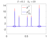
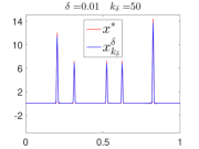
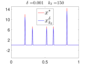
Fig. 1: Reconstruction results for Section 3.1.

3.2 Two-dimensional TV deblurring

In this and next subsections we test the performance of Algorithm 1 on image deblurring problems whose objective is to reconstruct the unknown true image $x^{*}\in{\mathbb{R}}^{M\times N}$ from an observed image $b^{\delta}=Ax^{*}+\eta$ degraded by a linear blurring operator $A$ and a Gaussian noise $\eta$. We consider the case that the blurring operator is shift invariant so that $A$ is a convolution operator whose kernel is a point spread function.

This subsection concerns the total variation deblurring [44], assuming the periodic boundary conditions on images. To apply Algorithm 1, we take $W=\nabla$ to be the discrete gradient operator as used in [47, 48]. Correspondingly, the $x$-subproblem can be solved efficiently by the fast Fourier transform (FFT) and the $y$-subproblem has an explicit solution given by the soft-thresholding [47]. Therefore, Algorithm 1 can be efficiently implemented.

Figure 2 reports numerical results by Algorithm 1 on test images Cameraman ($256\times 256$) and Pirate ($512\times 512$) with motion blur (fspecial(’motion’,35,50)) and Gaussian blur (fspecial(’gaussian’,[20 20], 20)) respectively. The noise level are $\delta=0.256$ and $0.511$ respectively. As comparisons, we also include the results obtained by FTVd v4.1 in [47] which is a state-of-art algorithm for image deblurring. We can see that the images reconstructed by our proposed ADMM have comparable quality as the ones obtained by FTVd v4.1 with similar PSNR (peak sigal-to-noise ratio), while the choice of the regularization parameter is not needed in our algorithm. Here the PSNR is defined by

$$\mathrm{PSNR}=10\cdot\log_{10}\frac{255^{2}}{\mathrm{MSE}}[\mathrm{dB}],$$

where MSE stands for the mean-squared-error per pixel.

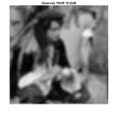
Fig. 2: ADMM-TV Debluring

3.3 Two-dimensional framelet deblurring

In this subsection we show the performance of Algorithm 1 for image deblurring using wavelet frames [6, 7, 14, 15, 46].

In our numerical simulations on grayscale digital images represented by $M\times N$ arrays, we will use the two-dimensional Haar with three level decomposition and piecewise linear B-spline framelets with one level decomposition, which can be constructed by taking tensor products of univariate ones [8]. The action of the discrete framelet transform and its adjoint on images can be implemented implicitly by the MRA-based algorithms [11]. Assuming the periodic boundary condition on images, the $x$-subproblem in Algorithm 1 then can be solved by FFT. The $y$-subproblem can be solved by the soft thresholding. Thus, Algorithm 1 can be efficiently implemented. Figure 3 reports the reconstruction results using the test images Phantom ($256\times 256$) and Peppers ($256\times 256$) with motion blur (fspecial(’motion’,50,90)) and Gaussian blur (fspecial(’gaussian’,[20 20], 30)) respectively. The noise leve is $\delta=0.256$ for two examples. These results indicate the satisfactory performance of our proposed ADMM.

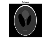
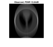
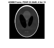
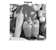
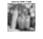
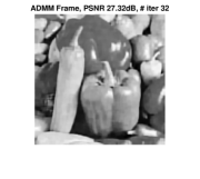
Fig. 3: ADMM-Framelet

3.4 Semi-convergence

In this subsection we investigate the numerical performance of our ADMM if it is not terminated properly. We use the 2-dimensional Cameraman TV deblurring as an example and run our ADMM until a preassigned maximum number of iterations (500) is achieved. In Figures 4 we plot the corresponding results on the PSNR values and the values of $E_{k}^{\delta}$ versus the number of iterations. It turns out that the PSNR increases first and then decreases after a critical number of iterations. This illustrates the semi-convergence property of our proposed ADMM in the framework of iterative regularization methods and indicates the importance of terminating the iteration by a suitable stop rule.

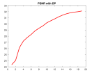
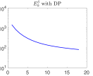
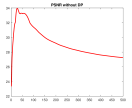
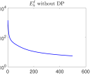
Stop by (45)		Nonstop

Fig. 4: Semi-convergence test

3.5 Sensitivity on $\rho_{1}$ and $\rho_{2}$

In this subsection we illustrate that the performance of Algorithm 1 is not quite sensitive to the two parameters $\rho_{1}$ and $\rho_{2}$. To this end we run our ADMM on the Cameraman TV deblurring problem with same parameters as in Section 3.2 with different $\rho_{1}$ and $\rho_{2}$. The PSNR and the number of iterations are given in Table 1 from which we can see that the reconstructions remain stable for a large range of values of $\rho_{1}$ and $\rho_{2}$.

Table 1: PSNR and number of iteration for different $\rho_{1}$ and $\rho_{2}$.

	250	500	1000	2000	4000
2.5	(31.9, 61 )	(32.1, 30 )	( 32.7, 15 )	(31.7, 9 )	(30.6, 5 )
5	(32.0, 64 )	(32.9, 33 )	( 32.4, 17 )	(31.6, 10 )	(31.5, 6 )
10	(32.5, 68 )	(33.0, 36 )	( 32.1, 20 )	(32.2, 11 )	(32.0, 7 )
20	(33.1, 74 )	(32.3, 40 )	( 32.5, 23 )	(32.7, 14 )	(32.4, 9 )
40	(32.8, 82 )	(32.6, 47 )	( 32.8, 28 )	(32.5, 17 )	(32.0, 11 )
80	(32.7, 97 )	(32.9, 58 )	( 32.8, 36 )	(32.3, 23 )	(31.6, 15 )
160	(32.9, 120 )	(32.9, 76 )	( 32.5, 50 )	(31.9, 34 )	(31.3, 24 )

4 Conclusion

In this work we propose an alternating direction method of multiplies to solve inverse problems. When the data is given exactly, we prove the convergence of the algorithm without using the existence of Lagrange multipliers. When the date contains noise, we propose a stop rule and show that our ADMM renders into a regularization method. Numerical simulations are given to show the efficiency of the proposed algorithm.

There are several possible extensions for this work. First, in our ADMM for solving inverse problems, we used two parameters $\rho_{1}$ and $\rho_{2}$ which are fixed during iterations. It is natural to consider the situation that $\rho_{1}$ and $\rho_{2}$ change dynamically. Variable step sizes have been used in the augmented Lagrangian method to reduce the number of iterations (see [20, 19, 34]). It would be interesting to investigate what will happen if dynamically changing parameters $\rho_{1}$ and $\rho_{2}$ are used in our ADMM. Second, the $x$-subproblem in our ADMM requires to solve linear systems related to $\rho_{1}A^{*}A+\rho_{2}W^{*}W$. In general, solving such linear system is very expensive. It might be possible to remedy this drawback by applying the linearization and/or precondition strategies. Finally, in applications where the sought solution is a priori known to satisfy certain constraints, it is of interest to consider how to incorporate such constraints into our ADMM in an easily implementable way and to prove some convergence results.

References

• [1] H. H. Bauschke and P. L. Combettes. Convex Analysis and Monotone Operator Theory in Hilbert Spaces. Springer Science & Business Media, 2011.
• [2] D. P. Bertsekas. Constrained Optimization and Lagrange Multiplier Methods. Academic press, 1982.
• [3] R. Boţ and T. Hein. Iterative regularization with a general penalty term – theory and application to ${L}^{1}$ and TV regularization. Inverse Problems, 28(10):104010, 2012.
• [4] S. Boyd, N. Parikh, E. Chu, B. Peleato, and J. Eckstein. Distributed optimization and statistical learning via the alternating direction method of multipliers. Foundations and Trends® in Machine Learning, 3(1):1–122, 2011.
• [5] L. M. Bregman. The relaxation method of finding the common point of convex sets and its application to the solution of problems in convex programming. USSR Comput. Math. Math. Phys., 7(3):200–217, 1967.
• [6] J.-F. Cai, B. Dong, S. Osher, and Z. Shen. Image restoration: total variation, wavelet frames, and beyond. J. Amer. Math. Soc., 25(4):1033–1089, 2012.
• [7] J.-F. Cai, B. Dong, and Z. Shen. Image restorations: a wavelet frame based model for piecewise smooth functions and beyond. Preprint, 2014.
• [8] A. Chai and Z. Shen. Deconvolution: a wavelet frame approach. Numer. Math., 106(4):529–587, 2007.
• [9] A. Chambolle and T. Pock. A first-order primal-dual algorithm for convex problems with applications to imaging. J. Math. Imaging Vis., 40(1):120–145, 2011.
• [10] J. B. Conway. A Course in Functional Analysis, volume 96. Springer Science & Business Media, 1990.
• [11] I. Daubechies, B. Han, A. Ron, and Z. Shen. Framelets: MRA-based constructions of wavelet frames. Appl. Comput. Harmon. Anal., 14(1):1–46, 2003.
• [12] D. Davis and W. Yin. Convergence rates of relaxed peaceman-rachford and admm under regularity assumptions. arXiv preprint arXiv:1407.5210, 2014.
• [13] W. Deng and W. Yin. On the global and linear convergence of the generalized alternating direction method of multipliers. Technical report, DTIC Document, 2012.
• [14] B. Dong, Q. Jiang, and Z. Shen. Image restoration: wavelet frame shrinkage, nonlinear evolution pdes, and beyond. UCLA CAM Report, 13:78, 2013.
• [15] B. Dong and Z. Shen. MRA-based wavelet frames and applications. IAS Lecture Notes Series 19, Summer Program on “The Mathematics of Image Processing”, Park City Mathematics Institute, 2010.
• [16] J. Eckstein and D. P. Bertsekas. On the douglas-rachford splitting method and the proximal point algorithm for maximal monotone operators. Math. Program., 55(1-3):293–318, 1992.
• [17] H. W. Engl, M. Hanke, and A. Neubauer. Regularization of Inverse Problems, volume 375. Springer Science & Business Media, 1996.
• [18] K. Frick and M. Grasmair. Regularization of linear ill-posed problems by the augmented Lagrangian method and variational inequalities. Inverse Problems, 28(10):104005, 2012.
• [19] K. Frick, D. A. Lorenz, and E. Resmerita. Morozov’s principle for the augmented Lagrangian method applied to linear inverse problems. Multiscale Model. Simul., 9(4):1528–1548, 2011.
• [20] K. Frick and O. Scherzer. Regularization of ill-posed linear equations by the non-stationary augmented Lagrangian method. J. Integral Equations Appl., 22(2):217–257, 2010.
• [21] D. Gabay. Applications of the method of multipliers to variational inequalities. Studies in Mathematics and its Applications, 15:299–331, 1983.
• [22] D. Gabay and B. Mercier. A dual algorithm for the solution of nonlinear variational problems via finite element approximation. Computers & Mathematics with Applications, 2(1):17–40, 1976.
• [23] V. Girault and P. A. Raviart. Finite Element Approximation of the Navier-Stokes Equations, volume 749 of Lecture Notes in Math. Springer-Verlag, 1979.
• [24] R. Glowinski and A. Marroco. Sur l’approximation, par éléments finis d’ordre un, et la résolution, par pénalisation-dualité d’une classe de problèmes de dirichlet non linéaires. ESAIM: Math. Model. Numer. Anal., 9(R2):41–76, 1975.
• [25] B. He, H. Liu, Z. Wang, and X. Yuan. A strictly contractive peaceman–rachford splitting method for convex programming. SIAM J. Optim., 24(3):1011–1040, 2014.
• [26] B. He and X. Yuan. Convergence analysis of primal-dual algorithms for a saddle-point problem: from contraction perspective. SIAM J. Imaging Sci., 5(1):119–149, 2012.
• [27] B. He and X. Yuan. On the o(1/n) convergence rate of the douglas-rachford alternating direction method. SIAM J. Numer. Anal., 50(2):700–709, 2012.
• [28] M. R. Hestenes. Multiplier and gradient methods. J. Optim. Theory Appl., 4:303–320, 1969.
• [29] M. Hong and Z.-Q. Luo. On the linear convergence of the alternating direction method of multipliers. arXiv preprint arXiv:1208.3922, 2012.
• [30] K. Ito and B. Jin. Inverse Problems: Tikhonov Theory and Algorithms. World Scientific, Singapore, 2014.
• [31] Q. Jin and X. Lu. A fast nonstationary iterative method with convex penalty for inverse problems in Hilbert spaces. Inverse Problems, 30(4):045012, 2014.
• [32] Q. Jin and W. Wang. Landweber iteration of Kaczmarz type with general non-smooth convex penalty functionals. Inverse Problems, 29(8):085011, 2013.
• [33] Q. Jin and H. Yang. Levenberg-marquardt method in baach spaces with general convex regularization terms. Numer. Math., published online: 08 September 2015.
• [34] Q. Jin and M. Zhong. Nonstationary iterated Tikhonov regularization in Banach spaces with uniformly convex penalty terms. Numer. Math., 127(3):485–513, 2014.
• [35] Q. Li, L. Shen, Y. Xu, and N. Zhang. Multi-step fixed-point proximity algorithms for solving a class of optimization problems arising from image processing. Adv. in Comput. Math., pages 1–36, 2014.
• [36] P.-L. Lions and B. Mercier. Splitting algorithms for the sum of two nonlinear operators. SIAM J. Numer. Anal., 16(6):964–979, 1979.
• [37] J. Locker and P. Prenter. Regularization with differential operators 1: general theory. J. Math. Anal. Appl., 74:504–529, 1980.
• [38] V. A. Morozov. Methods for Solving Incorrectly Posed Problems. Springer, New York, Berlin, Heidelberg, 1984.
• [39] V. A. Morozov and M. Stessin. Regularization methods for ill-posed problems. Crc Press Boca Raton, FL:, 1993.
• [40] S. Osher, M. Burger, D. Goldfarb, J. Xu, and W. Yin. An iterative regularization method for total variation-based image restoration. Multiscale Model. Simul., 4(2):460–489, 2005.
• [41] M. J. D. Powell. A method for nonlinear constraints in minimization problems. in Optimization ed. by R. Fletcher, pages 283–298, 1969.
• [42] R. T. Rockafellar. The multiplier method of Hestenes and Powell applied to convex programming. J. Optim. Theory Appl., 12(6):555–562, 1973.
• [43] R. T. Rockafellar. Augmented Lagrangians and applications of the proximal point algorithm in convex programming. Mathematics of Operations Research, 1(2):97–116, 1976.
• [44] L. I. Rudin, S. Osher, and E. Fatemi. Nonlinear total variation based noise removal algorithms. Physica D: Nonlinear Phenomena, 60(1):259–268, 1992.
• [45] T. Schuster, B. Kaltenbacher, B. Hofmann, and K. S. Kazimierski. Regularization Methods in Banach Spaces, volume 10. Walter de Gruyter, 2012.
• [46] Z. Shen. Wavelet frames and image restorations. ”Proceedings of the International Congress of Mathematicians”, India, 2010.
• [47] Y. Wang, J. Yang, W. Yin, and Y. Zhang. A new alternating minimization algorithm for total variation image reconstruction. SIAM J. Imaging Sci., 1(3):248–272, 2008.
• [48] X. Zhang, M. Burger, and S. Osher. A unified primal-dual algorithm framework based on Bregman iteration. J. Sci. Comput., 46(1):20–46, 2011.