Abstract

We provide an alternative formulation of the exact calculation of the current-voltage characteristic of solar cells which have been modeled with a lumped parameters equivalent circuit with one or two diodes. Such models, for instance, are suitable for describing organic solar cells whose current-voltage characteristic curve has an inflection point, also known as an S-shaped anomaly. Our formulation avoids the risk of numerical overflow in the calculation. It is suitable for implementation in Fortran, C or on micro-controllers.

1   Introduction

The current-voltage characteristic of a solar cell is often modeled using an equivalent circuit with lumped parameters. Different models use one, two or three diodes in the circuit. These models have an associated implicit equation which relates the current and voltage measurements, and parameters which can be adjusted to make the model fit experimental data. The implicit equations for some models can be solved explicitly to obtain an exact equation $V=f(I)$ by which the voltage $V$ can be calculated from the current $I$.

Some of the formulas for the equation $V=f(I)$, as they are usually written, involve intermediate calculations which, if not handled properly, may produce arithmetic overflow. Overflow may happen even if the calculation is done using double or quadruple precision hardware floating point arithmetic. It may be necessary to use special software, such as a symbolic mathematics package or a subroutine library for multi-precision arithmetic, in order to calculate some of the formulas for $V=f(I)$ as usually written. That can restrict the applicability of the explicit formula to situations which have appropriate computer software resources.

The purpose of this paper is to review some of the formulas for $V=f(I)$, and to rewrite them to avoid possible overflow. The rewritten formulas can be utilized in Fortran or C with hardware floating point, or on micro-processors with fixed point arithmetic, in order to calculate $V=f(I)$ with little risk of overflow. That enables the explicit formulas to be used in field implementations, such as in test equipment for solar cells, or for load balancing of solar energy installations. There is no need to have a Lambert W function implementation in the Fortran, C, or micro-processor environment. We give a simple algorithm for calculation of an analytic function $y=g(x)$ which serves the same purpose.

We will start with the one diode model in section 2. That model is often used for non-organic solar cells. We show how one can rewrite a $V=f(I)$ formula to avoid overflow. Rewriting of the one diode $V=f(I)$ formula for computational robustness lays the groundwork for considering the two diode model situation.

In section 4 we will turn to a particular two diode model. For some organic solar cells the experimentally measured $I-V$ characteristic curve may have an inflection point, also called an S-shaped anomaly. A two diode model can be used to represent the shape of the $I-V$ curve and to achieve a good fit of the model to the observational data. An inflection point is frequently associated with poor performance of the organic solar cell. The inflection point can be altered, or even removed, by annealing of the solar cell. Having a good analytic formula $V=f(I)$ for the $I-V$ characteristic may be helpful for understanding how the annealing process works. As well, because two diode models have more parameters than the one diode model, it may not be as easy to use numerical search techniques to identify the relevant subspace of physically achievable solar cells.

Our primary objective in this paper is to obtain methods that will assist with the computational tasks associated with investigation of organic solar cells, in particular using two diode models. We also expect that our methods will be useful for field implementations of load balancing for solar panel arrays of solar cells, using either one or two diode models.

2   One Diode Model

Solar cells can be modeled via an equivalent circuit with lumped parameters and a single diode [1], as shown in figure 1. This model is described by an implicit equation which relates the current $I$ and the voltage $V$ in terms of the cell parameters:

$$I=I_{0}\,\Big{(}\mathrm{exp}\Big{[}\frac{q}{nk_{B}T}(V-IR_{s})\Big{]}-1\Big{)}+\frac{V-IR_{s}}{R_{sh}}-I_{ph},$$ (1)

where $I_{ph}$ is the cell’s photocurrent, $I_{0}$ is the diode’s reverse saturation current, $n$ is the diode’s ideality factor, $R_{s}$ is the series resistance, $R_{p}$ is the parallel (shunt) resistance, $q$ is the magnitude of the electron charge, $k_{B}$ is Boltzmann’s constant, and $T$ is absolute temperature. Here we have written the current $I$ with the opposite sign to the current convention on pp 14-15 of [1]. As well, we have assumed unit solar cell area, so that we speak of current rather than current areal density. This model is descriptive of the solar cell under some assumed standard illumination, appropriate for the experimental tests which provide the $I,V$ data points. The photocurrent generated within the solar cell under illumination is represented by $I_{ph}$.

Figure 1: One diode model of a solar cell.
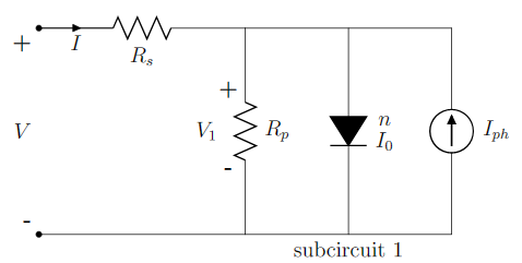
Diode reverse saturation current $I_{0}$ and ideality factor $n$.
————————————————————————————–

This one diode model is adequate for the description of many solar cells. The implicit equation (1) can be solved to obtain an explicit equation for $I$ as a function of $V$, or an explicit equation for $V$ as a function of $I$ [2]. Here we will focus on just the explicit equation for $V$ as a function of $I$, as that is the form which is used in two diode models.

Jain and Kapoor [2] give an exact explicit formula for $V$ as a function of $I$. In our notation and with our sign convention, their formula is

$$V=f(I) = IR_{s}+(I+I_{ph}+I_{0})R_{p}$$ (2)

$$- \frac{nk_{B}T}{q}W\Big{(}\frac{q}{nk_{B}T}I_{0}R_{p}\mathrm{exp}\Big{[}\frac{q}{nk_{B}T}R_{p}(I+I_{ph}+I_{0})\Big{]}\Big{)}$$

The function $W$ is the Lambert W function [3, 4, 5]. The principal branch of that function is used in these calculations since the argument to $W$ is a positive real value and the result is also to be a real value.

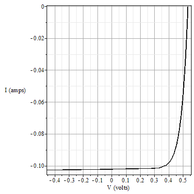
Suppose we consider a solar cell with parameters $I_{ph}=0.1023$ amp, $I_{0}=0.1036\times 10^{-6}$ amp, $n=1.5019$, $R_{s}=0.06826$ ohm, $R_{p}=1000$ ohms, at $T=300$ K. These values are the parameters obtained in [6] for the experimental data for the “blue” solar cell. The original experimental data, and the previous model fit via solution of an equivalent of the implicit equation (1), are reported in [7]. The $I-V$ characteristic curve for this fitted model with the above parameters from reference [6] is shown in figure 2.

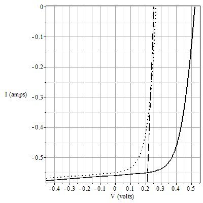
As a second example, we consider another solar cell, the “grey” solar cell, which was also experimentally studied and fitted, with results reported in [7] and further considered in [6]. The parameters obtained in [6] for the grey solar cell are $I_{ph}=0.5610$ amp, $I_{0}=5.514\times 10^{-6}$ amp, $n=1.7225$, $R_{s}=0.07769$ ohm, $R_{p}=25.9$ ohms, at $T=307$ K. The $I-V$ characteristic of the fitted model of the grey solar cell is shown as the solid curve in figure 3.

Figure 2: I-V characteristic for the one diode model of the “blue” solar
cell of [7], calculated from the fitted parameters described in [6].
————————————————————————————-

If the $I-V$ characteristic curve for the blue solar cell, graphed in figure 2, were to be calculated using the formula given in equation (2) using IEEE-754-2008 standard [8] hardware floating point in double precision, there would be an arithmetic overflow exception. For a current $I=0$, the argument of the $W()$ function is $4.59\times 10^{1141}$. The maximum representable magnitude in IEEE-754-2008 compliant double precision is about $10^{323}$. One might use quadruple precision floating point, referred to in the standard as “binary128”, as it is able to represent magnitudes up to about $10^{5107}$. However, as we will see with another example below, also using model parameters which were obtained via fitting the two diode model to experimental data from an actual solar cell, even quadruple floating point arithmetic can be insufficient to avoid overflow during the calculation of the $V=f(I)$ function via a formula such as that written in equation (2).

On the other hand, the calculation of the grey solar cell’s characteristic curve, shown in figure 3, would not produce an arithmetic overflow. The maximum magnitude involved in the calculation of that curve via formula (2) is about $3\times 10^{138}$, even for intermediate variables involved in the calculation. That is compatible with the limitations of standard-compliant hardware double precision arithmetic.

Figure 3: I-V characteristic for the one diode model of the “grey” solar
cell of [7], calculated from the fitted parameters described in [6].
Shows the two components of the model; a sloped straight line
and a “J”-shape representing the scaled $g(x)$ function.
The sum of these two components is the grey cell’s $I-V$ curve.
————————————————————————————-

How is one to know when it is safe to use formula (2) for a calculation? The blue solar cell is not an anomaly. In fact, the authors of the original study [7] consider the blue cell to be of better quality compared to the grey cell. The blue cell has a larger fill factor, lower series resistance, higher shunt resistance, and lower ideality factor.

Higher shunt resistance in the lumped parameters model is associated with improvements in solar cell quality. However, higher shunt resistance also increases the numerical magnitude of the Lambert W function argument in formula (2). Solar cells are better now, three decades after the study [7]. Thus one can expect to encounter actual solar cells whose model parameters will produce arithmetic overflow if the formula (2) is applied in a standard computer language such as Fortran or C, or if an implementation of that formula is attempted on a micro-controller.

How did the authors of the studies [7] and [6] utilize the model parameters they derived? They did not use the explicit formula (2), instead relying upon solving the implicit equation (1), and other approximation techniques. One would like, however, to be able to use a explicit and exact formula such as (2) because it is analytic, that is has derivatives of all orders, and hence can be used in optimization studies and other investigations. What is desired is to obtain a formula to replace (2) which is exact, explicit and analytic, yet is also robust when used in calculations, and does not pose a risk of arithmetic overflow. Such a formula is desirable both for laboratory studies, and for industrial applications (test equipment for a manufacturing line) and field installations (load balance). It should be suitable for programming in Fortran or C, or on micro-controllers which may have only a fixed point arithmetic software package.

A related concern is possible cancellation causing loss of significant digits in the result. Equation (2) involves some subtractions. For $I=0$ for the blue solar cell, we have a value of 102.300 for the linear terms, from which is subtracted a value 101.764 representing the scaled value of the Lambert W function, causing a loss of about two significant digits. Cancellation is not problematic in this instance. However, if there were a way to reduce cancellation while rewriting the formula (2), that would be desirable.

Examples such as these have motivated our introduction of an alternative technique for calculating a function like $V=f(I)$ as defined by equation (2). In the next section, we use the function $g(x)=\mathrm{log}(W(e^{x}))$ which was described in a previous note [9], and rewrite the formula $V=f(I)$ given by (2) in terms of the function $g(x)$. Here $\mathrm{log}$ denotes the natural logarithm (base $e$) function, the inverse of the exponential function.

3   Rewrite of Equation (2) Formula

First, we make the general observation that the function $g(x)$ satisfies

$$g(x)=\mathrm{log}(W(e^{x}))=x-W(e^{x}).$$ (3)

This fact is obtained in [10] as the equivalence of equations (32) and (37) of that paper. To verify equation (3) directly, it suffices to take the exponential of both sides of (3) , multiply out, and use the defining property of the Lambert W function, that $W(z)\,e^{W(z)}=z$. Hence, when we have a formula containing an expression of the form $x-W(e^{x})$ we can replace it by calculation of the function $g(x)$. The two forms are mathematically equivalent, but the form $x-W(e^{x})$ has a risk of arithmetic overflow when the argument $e^{x}$ to the $W()$ function is calculated. There is also a risk of possible cancellation causing loss of significant digits when the subtraction is performed. The function $g(x)$ is well-behaved in numerical calculations.

The function $y=g(x)$ is just the principal branch of the real values of the Lambert W function in another coordinate system. We have $e^{y}=W(e^{x})$. Thus if the function $w=W(z)$, with $w$ and $z$ restricted to positive real values, were to be graphed on log-log axes, we would see the graph of the $y=g(x)$ function. The distinction between the two functions is not in their mathematical properties, but in their computational practicality. In section 5 below we describe how to compute $g(x)$ without overflow. Further details and discussion of the function $g(x)$ are given in reference [9].

We wish to recast (2) to evaluate $W(e^{x})$ for some $x$. Clearly we should write

$$x=\mathrm{log}\Big{[}\frac{q}{nk_{B}T}\,I_{0}R_{p}\Big{]}+\frac{q}{nk_{B}T}\,R_{p}\,(I+I_{ph}+I_{0}).$$ (4)

Transposing the $IR_{s}$ term in equation (2) and multiplying by $\frac{q}{nk_{B}T}$ we obtain

$$\frac{q}{nk_{B}T}\,(V-IR_{s}) = \frac{q}{nk_{B}T}\,(I+I_{ph}+I_{0})\,R_{p}-W(e^{x})$$

$$= \Big{(}x-\mathrm{log}\Big{[}\frac{q}{nk_{B}T}\,I_{0}R_{p}\Big{]}\Big{)}-W(e^{x})$$

$$= g(x)-\mathrm{log}\Big{[}\frac{q}{nk_{B}T}\,I_{0}R_{p}\Big{]}.$$

That is,

$$\frac{q}{nk_{B}T}\,(V-IR_{s})+\mathrm{log}\Big{[}\frac{q}{nk_{B}T}\,I_{0}R_{p}\Big{]}=g(x).$$ (5)

Consider the geometric content of equations (4) and (5). Equation (4) says that the value of the variable $x$ is obtained by a linear shift and scale change of the current $I$. Equation (5) says that the value of the function $g(x)$ is obtained by a linear shift and scale change of the subcircuit 1 voltage drop $V_{1}=V-IR_{s}$. Hence we expect the graph of $V_{1}=V-IR_{s}=f(I)-IR_{s}$ to look like the graph of $y=g(x)$, but with a shift of origin and with linear scale changes on the two axes.

Figures 4 and 5 show the graph of $y=g(x)$ at two different magnifications. From close up, $-4\leq x\leq 4$ in figure 4, the graph looks like a smooth curve going through the point $(1,0)$ near the origin. From far away, $-1000\leq x\leq 1000$ in figure 5, the graph looks like a pair of straight lines, represented by an abrupt change in slope at the origin. Which picture we use for matching with a part of the $V-IR_{s}=f(x)-IR_{s}$ curve, that is either a smooth curve or a pair of straight lines joined at what appears to be a sharp corner, depends upon the particular scales used for $I$ and $V$. That behavior is of course modified by the physical limitations on the voltages and currents within the device being modeled. However, regardless of appearance, whether a smooth curve or joined straight lines, the function $g(x)$ is analytically smooth. That is, $g(x)$ has an unlimited number of derivatives, and one can use it to determine extrema or inflection points, and so on.

Figure 4: Graph of $y=g(x)=\mathrm{log}(W(\mathrm{exp}(x)))$
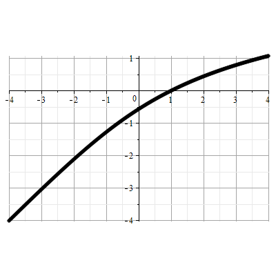
for moderate magnitudes of the argument.
——————————————————————————–

Figure 5: Graph of $y=g(x)=\mathrm{log}(W(\mathrm{exp}(x)))$
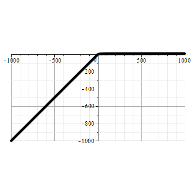
for large magnitudes of the argument.
——————————————————————————–

The voltage $V$ across the solar cell is given in terms of the function $g(x)$, using the variable $x$ which is a transformation of the current $I$, and is calculated as

$$V=I\,R_{S} + n\,\frac{k_{B}T}{q}\,g(x)$$ (6)

$$- \frac{nk_{B}T}{q}\mathrm{log}\Big{[}\frac{q}{nk_{B}T}\,I_{0}R_{p}\Big{]}.$$

Equation (6), with the ancillary equation (4) to define $x$, is our proposed replacement for the formula (2). The function $g(x)$ is to be implemented as described in section 5. The two formulas (2) and (6) are mathematically equivalent, and each of them explicitly calculates $V=f(I)$, the exact solution for the one diode model. The formulas differ, however, in that our proposed formula is unlikely to experience overflow, and will likely have less cancellation error.

When graphing the blue solar cell’s $I-V$ curve to obtain figure 2, formula (2) can have intermediate values as large as $1.7\times 10^{1144}$ in magnitude, which will produce arithmetic overflow in standard-compliant hardware double precision arithmetic. In contrast, the calculation of this graph using formulas (4) and (6) involves intermediate values only up to 3000 in magnitude. For the grey solar cell, the calculation of the graph in figure 3 using the rewritten formulas involves intermediate values only up to 400 in magnitude, whereas the original formula involved intermediate values more than $10^{138}$ in magnitude. These low magnitudes of intermediate variables in calculating formulas (4) and (6) hold for the calculations within both the portion of the code which implements the evaluation of the $g(x)$ function itself, and the portion of the code which carries out the rest of the work in formulas (4) and (6). The magnitudes in the latter portion of the code can of course be adjusted by a suitable choice of units. The $g(x)$ function is in essence a black box, just as the Lambert W function was a black box in formula (2). It is important, when one is going to use a black box function, that it be reliable.

The moderate magnitudes of the intermediate values involved in computing the $V=f(I)$ function using the $g(x)$ function indicates the rewritten formula’s suitability for implementation in fixed point arithmetic, such as on a micro-controller.

We can visualize formula (6) geometrically as the sum of two curves, a sloped straight line plus a copy of the $y=g(x)$ curve. First, recognize that we are graphing $V=f(I)$ with the $V$ axis horizontal and the $I$ axis vertical, so the copy of the $y=g(x)$ curve should be flipped over the diagonal line $y=x$, to put $y$ horizontal and $x$ vertical. The $IR_{s}$ first term in (6), with axes flipped, is a straight line with slope $\frac{1}{R_{s}}$ through the origin, and becomes steeper if the series resistance is lower. The third term in (6), the $\mathrm{log}()$ term, is simply a shift of that straight line left or right (or up or down). The second term of (6) is the addition of a copy of the flipped $y=g(x)$ curve proportional to the ideality factor $n$. Addition of a flipped copy of the $y=g(x)$ curve provides the J-shape of the $I-V$ curve.

This discussion of the method of rewriting the one diode model lays the groundwork for rewriting of the formulas used for two diode models. We will see that similar techniques are applicable. The matching of $I-V$ characteristics with one or two inflection points can be interpreted as finding the appropriate scaling and shift parameters for adding or subtracting flipped copies of the $g(x)$ function graph to a sloped straight line representing the series resistance.

Methodological Note: The reader may wish to know how the above-mentioned intermediate value magnitudes in calculations were obtained. We implemented the formulas (2), (4) and (6) in a software package which does not have a limitation on numerical magnitudes. We inserted “probe” code at various points in the calculations, in order to record the magnitudes of the intermediate values of interest. These probe magnitudes were fed through a high-water-mark filter, and recorded in global variables. After a set of calculations, such as the preparation of a graph like figures 2 or 3, the global variables were inspected to determine the peak magnitudes which were involved in the calculations. That enabled us to determine whether a hardware implementation of the calculation would have produced arithmetic overflow.

4   Two Diode Model

The current-voltage characteristic of some organic solar cells shows an inflection point, also known as an “S-shape anomaly”. This has been modeled by a lumped parameters equivalent circuit using two or three diodes. Each model’s equivalent circuit has an implicit equation relating the current $I$ and voltage $V$. Some of these model configurations are amenable to obtaining exact and explicit formulas of the form $V=f(I)$, utilizing the Lambert W function. In this section we will consider a particular two diode model, and discuss the rewriting of its formulas to reduce the risk of arithmetic overflow during calculations. Having an explicit function is useful because it enables rapid and exact calculation of the $I-V$ curve given values of the parameters of the model. Further the explicit function is analytic so it can be used to perform optimization investigations. There may be eight (or more) parameters in a multi-diode model, so numerical random search optimization methods may be time consuming in comparison to analytic methods.

Romero, et al [11] and García-Sánchez, et al [12] have considered a two diode model with a reverse-bias second diode and shunt resistor, as shown in figure 6. They give an exact solution utilizing eight parameters, which we will write as

$$V = f(I)=(I+I_{ph}+I_{01})\,R_{p1}$$ (7)

$$- \frac{n_{1}k_{B}T}{q}\,W\Big{\{}\frac{q}{n_{1}k_{B}T}\,I_{01}R_{p1}\,\mathrm{exp}\Big{[}\frac{q}{n_{1}k_{B}T}\,R_{p1}\,(I+I_{ph}+I_{01})\big{]}\Big{\}}$$

$$+ \frac{n_{2}k_{B}T}{q}\,W\Big{\{}\frac{q}{n_{2}k_{B}T}\,I_{02}R_{p2}\,\mathrm{exp}\Big{[}\frac{-q}{n_{2}k_{B}T}\,R_{p2}\,(I-I_{02})\Big{]}\Big{\}}$$

$$+ (I-I_{02})\,R_{p2}+IR_{s}$$

Figure 6: Two diode model of a solar cell, as in references [11, 12].
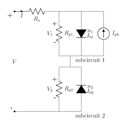
Subcircuit 1 has the photocurrent source, and a diode
with reverse saturation current $I_{01}$ and ideality factor $n_{1}$.
Subcircuit 2 has a reverse bias diode and a shunt resistance.
————————————————————————————–

We refer to the paper [11] for the derivation. All eight model parameters $I_{ph},R_{s},I_{01},R_{p1},n_{1},I_{02},R_{p2},n_{2}$ are positive numbers, except for $R_{s}$ which can be positive or zero.

An example of the S-shape anomaly (inflection point) can be seen in figure 7, which has been calculated from the model parameters obtained by Romero, et al [11] for a particular actual organic solar cell whose test data was fitted with their model. The parameter values used for that figure are $I_{ph}=4.85\,\times\,10^{-5}$ amp (photocurrent); $R_{s}=0$ ohm (series resistance assumed equal to zero); $I_{01}=1.5\,\times\,10^{-5}$ amp (primary diode reverse saturation current); $R_{p1}=1.0\,\times\,10^{8}$ ohms (primary diode shunt resistance); $n_{1}=2.4$ (primary diode ideality factor); $I_{02}=2.4\,\times\,10^{-7}$ amp (secondary diode reverse saturation current); $R_{p2}=4.6\,\times\,10^{4}$ ohms (secondary diode shunt resistance); $n_{2}=9.5$ (secondary diode ideality factor). The $I$ values range between about $-5.5\,\times\,10^{-5}$ amp and $0.1\,\times\,10^{-5}$ amp, and the corresponding $V$ values range between about -0.42 volt and 0.42 volt.

Figure 7: Graph of $V=f(I)$ for two diode model of organic solar cell.
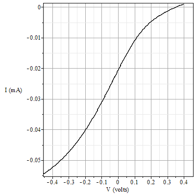
The axes are switched; that is, $I$ is vertical and $V$ is horizontal.
Agrees with best-fit curve shown in figure 2 of reference [11].
——————————————————————————–

The presence of an S-shape anomaly has been observed in organic solar cells produced by a variety of methods, and is associated with poor performance of the device. See [13] for background and for numerous references to examples of organic solar cells manufactured by various methods. The authors of [13] also explore the effect of annealing on changes in the inflection point of a solar cell. It is desirable to investigate the effect of annealing on changes in the model parameters of an organic solar cell, using the various two and three diode models available. It should be mentioned that S-shape anomalies can also be seen in non-organic solar cells. For instance, a recent paper [14] on a silicon quantum dot solar cell shows, in its figure 3, an inflection point in the $I-V$ characteristic of the test device.

As with the one diode model, there can be arithmetic overflow when the formula (7) is used for calculations. Hence it is desirable to rewrite the formula using the $g(x)$ function.

The primary diode circuit (subcircuit 1 in figure 6) is given by an equation identical to that used for a one diode model, with $V_{1}$ denoting the voltage drop across that subcircuit. That is (formula (8) of [11]),

$$V_{1} = f_{1}(I)=(I+I_{ph}+I_{01})\,R_{p1}$$ (8)

$$- \frac{n_{1}k_{B}T}{q}\,W\Big{\{}\frac{q}{n_{1}k_{B}T}\,I_{01}R_{p1}\,\mathrm{exp}\Big{[}\frac{q}{n_{1}k_{B}T}\,R_{p1}\,(I+I_{ph}+I_{01})\Big{]}\Big{\}}$$

This formula can be re-written just as for the one diode model. We obtain

$$x_{1}=\mathrm{log}\Big{[}\frac{q}{n_{1}k_{B}T}\,I_{01}R_{p1}\Big{]}+\frac{q}{n_{1}k_{B}T}\,R_{p1}\,(I+I_{ph}+I_{01}).$$ (9)

and

$$\frac{q}{n_{1}k_{B}T}\,V_{1}+\mathrm{log}\Big{[}\frac{q}{n_{1}k_{B}T}\,I_{01}R_{p1}\Big{]}=g(x_{1}).$$ (10)

Letting $V_{2}$ equal the voltage drop across subcircuit 2, which includes the reverse bias diode and shunt resistance, equation (9) of [11] is a comparable situation, with no photocurrent source. That is,

$$V_{2} = f_{2}(I)=(I-I_{02})\,R_{p2}$$ (11)

$$+ \frac{n_{2}k_{B}T}{q}\,W\Big{\{}\frac{q}{n_{2}k_{B}T}\,I_{02}R_{p2}\,\mathrm{exp}\Big{[}\frac{-q}{n_{2}k_{B}T}\,R_{p2}\,(I-I_{02})\Big{]}\Big{\}}$$

That formula also can be rewritten. We let

$$x_{2}=\mathrm{log}\Big{[}\frac{q}{n_{2}k_{B}T}\,I_{02}R_{p2}\Big{]}-\frac{q}{n_{2}k_{B}T}\,R_{p2}\,(I-I_{02}).$$ (12)

The result is

$$-\frac{q}{n_{2}k_{B}T}\,V_{2}+\mathrm{log}\Big{[}\frac{q}{n_{2}k_{B}T}\,I_{02}R_{p2}\Big{]}=g(x_{2}).$$ (13)

Once again we see that equations (12) and (13) represent the relationship between $I$ and $V_{2}$ in subcircuit 2 as a shift of origin and scale change of the current $I$, related to a shift of origin and scale change of the voltage $V_{2}$, the relationship being given by the function $y=g(x)$. The origin shifts and scale changes are however different from those for subcircuit 1, both for the current transformations and for the voltage transformations.

The two origin shifts and scale changes for the current are given by equations (9) and (12). The two origin shifts and scale changes for the voltage are given by equations (10) and (13).

The voltage $V$ across the solar cell is given by equation (1) of [11],

$$V=I\,R_{s}+V_{1}+V_{2}$$ (14)

In terms of the function $g(x)$, using the two variables $x_{1}$ and $x_{2}$ which are transformations of the current $I$, the voltage $V$ is calculated as

$$V=I\,R_{s} + n_{1}\,\frac{k_{B}T}{q}\,g(x_{1})-n_{2}\,\frac{k_{B}T}{q}\,g(x_{2})$$ (15)

$$- \frac{n_{1}k_{B}T}{q}\mathrm{log}\Big{[}\frac{q}{n_{1}k_{B}T}\,I_{01}R_{p1}\Big{]}$$

$$+ \frac{n_{2}k_{B}T}{q}\mathrm{log}\Big{[}\frac{q}{n_{2}k_{B}T}\,I_{02}R_{p2}\Big{]}.$$

Equation (15), with the ancillary equations (9) and (12) to define $x_{1}$ and $x_{2}$, is our proposed replacement for formula (7).

The new formula (15) produces the same $I-V$ characteristic curve as the original formula (7). The parameters above, used to draw figure 7, were obtained by the authors of [11] from a best fit of the two diode model to an actual solar cell, with the series resistance $R_{s}$ forced to zero. With these parameter values, in the original formula there would be arithmetic overflow even if hardware quadruple precision arithmetic were used, since the argument to one of the Lambert W function evaluations is about $10^{11232}$ when using the formula (7) at $I=0$. In contrast, for the new formula (15), there is no overflow since the maximum magnitude of an intermediate variable involved in the $g(x)$ function calculation is less than 30000, and the maximum magnitude of an intermediate variable involved in the overall $V=f(I)$ calculation of (15) is about $10^{8}$.

We can visualize the formula (15) geometrically as the sum of three curves, a sloped straight line plus two flipped copies of the $y=g(x)$ curve. One copy of the $y=g(x)$ curve, flipped, shifted, and scaled proportionally to the ideality factor $n_{1}$, is to be added; it represents the subcircuit 1 voltage $V_{1}$, the concave-up portion of the $I-V$ curve. The second copy of the $y=g(x)$ curve, flipped, shifted, and scaled proportionally to the ideality factor $n_{2}$, is to be subtracted; it represents the subcircuit 2 voltage $V_{2}$, the concave-down portion of the $I-V$ curve.

The authors of [12] have also proposed a three diode model which provides an improved fit for an organic solar cell with two inflection points in its $I-V$ characteristic curve. Their model presents some interesting computational challenges, related to assumptions regarding the ideality factors of the various diodes in the model. We have not considered, in this present paper, the applicability of our calculational methodology to the three diode model of [12]. We believe that represents an opportunity for further exploration.

5   Implementing the $y=g(x)$ Function

In this section, we describe the implementation of the calculation of the $y=g(x)$ function. See [9] for full details, including a discussion of the computational stability considerations. Here we present only a straightforward description of the necessary calculations to obtain $g(x)$.

Context: The function $y=g(x)=\mathrm{log}(W(\mathrm{exp}(x)))$ is to be calculated. The variable $x$ is a real number argument, positive or negative. The result variable $y$ is also a real number. See figures 4 and 5 for the graph of $y=g(x)$. The computer language should have available exponential and logarithm functions for the chosen precision, and a stored value of $e=\mathrm{exp}(1.0)$.

(a) Make an initial estimate $y_{0}$ of the result, as follows.

For $x\leq-e$, take $y_{0}=x$.

For $x\geq e$, take $y_{0}=\mathrm{log}(x)$.

For $-e<x<e$, take $y_{0}$ as a linear interpolation between the points $(-e,-e)$ and $(e,1)$. That is,

$$y_{0}=-e+\frac{1+e}{2e}\,(x+e)$$

This estimate $y_{0}$ is very crude. See figure 8 for a graph of the absolute error $g(x)-y_{0}$ for $-10<x<30$. The absolute error lies between -0.32 and +0.30.

Figure 8: Graph of $g(x)-y_{0}$ for approximation error
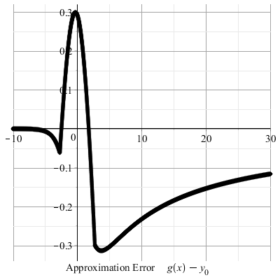
for initial estimate of g(x).
———————————————————————

(b) Refine the estimate $y_{0}$ by calculating

$$y_{1}=y_{0}-\frac{2(y_{0}+e^{y_{0}}-x)(1+e^{y_{0}})}{2(1+e^{y_{0}})^{2}-(y_{0}+e^{y_{0}}-x)e^{y_{0}}}.$$

This iteration formula is Halley’s method and has cubic convergence. See figure 9 for a graph of the absolute error $g(x)-y_{1}$ for $-10<x<30$. The absolute error lies between -0.001 and +0.00001.

Figure 9: Graph of $g(x)-y_{1}$ for approximation error
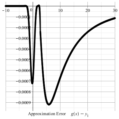
for first iterative refinement of estimate of g(x).
———————————————————————

(c) Further refine the estimate $y_{1}$ by calculating

$$y_{2}=y_{1}-\frac{2(y_{1}+e^{y_{1}}-x)(1+e^{y_{1}})}{2(1+e^{y_{1}})^{2}-(y_{1}+e^{y_{1}}-x)e^{y_{1}}}.$$

This second iteration produces an estimate which is good enough for most practical purposes. See figure 10 for a graph of the absolute error $g(x)-y_{2}$ for $-10<x<30$. The absolute error lies between $-10^{-10}$ and $+10^{-10}$.

The computational workload to obtain $y_{2}$ is two evaluations of the exponential function and one evaluation of the logarithm function.

Figure 10: Graph of $g(x)-y_{2}$ for approximation error
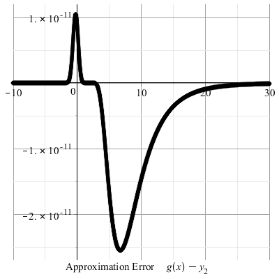
for second iterative refinement of estimate of g(x).
———————————————————————

(d) If the estimate $y_{2}$ is not precise enough for the intended application, perform additional iterations of the refinement formula,

$$y_{n+1}=y_{n}-\frac{2(y_{n}+e^{y_{n}}-x)(1+e^{y_{n}})}{2(1+e^{y_{n}})^{2}-(y_{n}+e^{y_{n}}-x)e^{y_{n}}}.$$

See figure 11 for a graph of the absolute error $g(x)-y_{3}$ after three iterations, for $-10<x<30$. The absolute error lies between $-10^{-33}$ and $+10^{-55}$.

Figure 11: Graph of $g(x)-y_{3}$ for approximation error
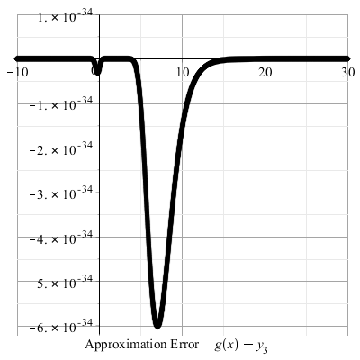
for third iterative refinement of estimate of g(x).
———————————————————————

Note: If examining the differences $|y_{n+1}-y_{n}|$ to determine if the result has converged, one should test for the absolute error, not the relative error. Because $y=0$ for $x=1$, a relative error test would be unreliable for $x$ in the vicinity of 1. Or, one might wish to code to test for absolute error if $|y_{n}|$ were less than 1, and for relative error for larger magnitudes of $|y_{n}|$.

The reason the above algorithm does not produce arithmetic overflow is that at no point is $\mathrm{exp}(x)$ calculated. Rather, the calculations involve only $x$, $y$, and $\mathrm{exp}(y)$. If hardware arithmetic underflow produces an error exception, instead of a zero result, then it will be desirable to code a test for negative values of $y_{n}$, for example $y_{n}<-100$, and simply stop iterating in that circumstance. Further discussion of the method is in reference [9].

6   Conclusion

We have suggested alternative formulas for computing the explicit function $V=f(I)$ which gives the exact current-voltage characteristic of the one or two diode models of a solar cell, in particular a solar cell with the S-curve property. The alternative formulas are less likely to produce arithmetic overflow errors when calculated with hardware floating point arithmetic. The alternative formulas are suitable for implementation in Fortran or C, or on micro-controllers.

We thank B. Romero and F. J. García-Sánchez for their helpful comments during our investigations.

References

- [1] Jenny Nelson, The Physics of Solar Cells. Imperial College Press, 2004.
- [2] Amit Jain, Avinashi Kapoor, “Exact analytical solutions of the parameters of real solar cells using Lambert W-function”. Solar Energy Materials and Solar Cells, vol 81 (2004), pp 269-277.
- [3] R. M. Corless, G. H. Gonnet, D. E. G. Hare, D. J. Jeffrey, D. E. Knuth, “On the Lambert W function”, Advances in Computational Mathematics, vol 5 (1996), pp 329-359.
- [4] S. R. Valluri, D. J. Jeffrey, R. M. Corless, “Some applications of the Lambert W function to physics”, Canadian Journal of Physics, vol 78, no 9 (September 2000), pp 823-831.
- [5] Frank Olver, et al (eds), NIST Handbook of Mathematical Functions, Cambridge, NIST, 2010. See page 111.
- [6] J. C. H. Phang, D. S. H. Chan, J. R. Phillips, “Accurate Analytical Method for the Extraction of Solar Cell Model Parameters”. Electronics Letters, vol 20, no 10 (10-May-1984), pp 406-408.
- [7] J. P. Charles, M. Abdelkrim, Y. H. Muoy, P. Mialhe, “A practical method of analysis of the current-voltage characteristics of solar cells”. Solar Cells, vol 4 (1981), pp 169-178.
- [8] IEEE, “IEEE Standard for Floating-Point Arithmetic”. IEEE 754-2008. Same technical content as the ISO/IEC/IEEE 60559:2011 standard. For a brief summary, see the Wikipedia article “IEEE floating point”.
- [9] Ken Roberts, “A Robust Approximation to a Lambert-Type Function”. ArXiv:1504.01964.
- [10] Francisco J. Garcia Sánchez, Adelmo Ortiz-Conde, Slavica Malobabic, “Aplicaciones de la Función de Lambert en Electrónica”. Universidad, Ciencia y Technología, volumen 10, número 40, septiembre 2006, pp 235-243.
- [11] B. Romero, G. del Pozo, B. Arredondo, “Exact analytical solution of a two diode circuit model for organic solar cells showing S-shape using Lambert W functions”. Solar Energy, vol 86 (2012), pp 3026-3029.
- [12] Francisco J. García-Sánchez, Denise Lugo-Muñoz, Juan Muci, Adelmo Ortiz-Conde, “Lumped Parameter Modeling of Organic Solar Cells’ S-Shaped I-V Characteristics”. IEEE Journal of Photovoltaics, vol 3, no 1 (January 2013), pp 330-335.
- [13] Mathilde R. Lilliedal, Andrew J. Medford, Morten V. Madsen, Kion Norrman, Frederik C. Krebs, “The effect of post-processing treatments on inflection points in current-voltage curves of roll-to-roll processed polymer photovoltaics”. Solar Energy Materials and Solar Cells, vol 94 (2010), pp 2018-2031.
- [14] Paresh Govind Kale, Chetan Singh Solanki, “Silicon quantum dot solar cell using top-down approach”. International Nano Letters, vol 5 (2015), pp 61-65.