Charged Perfect Fluid Sphere in Higher Dimensional Spacetime

Abstract

Present paper provides a new model for perfect fluid sphere filled with charge in higher dimensional spacetime admitting conformal symmetry. We consider a linear equation of state with coefficients fixed by the matching conditions at the boundary of the source corresponding to the exterior Reissner-Nordström higher dimensional spacetime. Several physical features for different dimensions, starting from four up to eleven, are briefly discussed. It is shown that all the features as obtained from the present model are physically desirable and valid as far as the observed data set for the compact star $SAX~{}J1808.4-3658~{}(SS2)$ is concerned.

1 Introduction

With the recent advancement in superstring theory in which the spacetime is considered to be of dimensions higher than four, the studies in higher dimensional spacetime has attained new importance. Throughout the last decade a number of articles have been published in this subject both in localized and cosmological domains. It is a common trend to believe that the $4$-dimensional present spacetime structure is the self-compactified form of manifold with multidimensions. Therefore, it is argued that theories of unification tend to require extra spatial dimensions to be consistent with the physically acceptable models Schwarz1985 ; Weinberg1986 ; Duff1995 ; Polchinski1998 ; Hellerman2007 ; Aharony2007 . It has been shown that some features of higher dimensional black holes differ significantly from $4$-dimensional black holes as higher dimensions allow for a much richer landscape of black hole solutions that do not have 4-dimensional counterparts Emparan2008 . Some recent higher dimensional works admitting one parameter Group of Conformal motion can be seen in the Refs. Pradhan2007 ; Khadekar2014 .

The study of charged fluid sphere has attained considerable interest among researchers in last few decades. It is observed that a fluid sphere of uniform density with a net surface charge becomes more stable than without charge stettner . According to Krasinski Krasinski in the presence of charge, the gravitational collapse of a spherically symmetric distribution of matter to a point singularity may be avoided. Sharma et al. sharma01 argue that in this situation the repulsive Colombian force counterbalances the gravitational attraction in addition to the pressure gradient. To study the cosmic censorship hypothesis and the formation of naked singularities Einstein-Maxwell solutions are also important joshi . The presence of charge affects the values for redshift, luminosity and maximum mass for stars. For a charged fluid spheres the gravitational field in the exterior region is described by Reissner-Nordström spacetime. Charged perfect fluid sphere satisfying a linear equation of state was discussed by Ivanov ivanov . In this paper the author reduced the system to a linear differential equation for one metric component. Regular models with quadratic equation of state was discussed by Maharaj and Takisa maharaj13 .

The obtained solutions of the Einstein-Maxwell system of equations are exact and physically reasonable. A physical analysis of the matter and electromagnetic variables indicates that the model is well behaved and regular. In particular there is no singularity in the proper charge density at the stellar center. A Charged anisotropic matter with linear equation of state has discussed by Thirukkanesh and Maharaj maharaj08 . In connection with this we want to mention a recent work of Varela et al. verela . In this paper the author considered a self-gravitating, charged and isotropic fluid sphere.

To solve Einstein-Maxwell field equation they have assumed both linear and nonlinear equation of state and discussed their result analytically. Rahaman et al. frahaman10 have obtained a singularity free solutions for anisotropic charged fluid sphere with Chaplygin equation of state. The authors used Krori-Barua ansatz kb to solve the system.

The well known inheritance symmetry is the symmetry under conformal killing vectors (CKV) i.e.

$$L_{\xi}g_{ik}=\psi g_{ik},$$ (1)

where $L$ is the Lie derivative of the metric tensor which describes the interior gravitational field of a compact star with respect to the vector field $\xi$ and $\psi$ is the conformal factor. In a deeper sense this inheritance symmetry provides the natural relationship between geometry and matter through the Einstein field equations. It is supposed that the vector $\xi$ generates the conformal symmetry and the metric $g$ is conformally mapped onto itself along $\xi$. Harko et al. Harko07 ; Harko08 have shown that neither $\xi$ nor $\psi$ need to be static even through one consider a static metric.

There are many earlier works on conformal motion in literature. The existence of one parameter group of conformal motion in Einstein-Maxwell spacetime have been studied in krori86a ; krori86b ; maartens . Anisotropic sphere admitting one-parameter group of conformal motion has been discussed by Herrera and León leon85a . A class of solutions for anisotropic stars admitting conformal motion has been studied in farook10 . Charged gravastar admitting conformal motion has been studied by Usmani et al. usmani11 . Bhar bhar1 has generalized this result in higher dimensional spacetime. Relativistic stars admitting conformal motion has been analyzed by Rahaman et al. rahaman10 . Isotropic and anisotropic charged spheres admitting a one parameter group of conformal motions was analyzed in leon85b . Anisotropic spheres admitting a one parameter group of conformal motions has been discussed by Herrera & León hleon85 . Charged fluid sphere with linear equation of state admitting conformal motion has been studied in Ref. aloma10 . The authors have also discussed about the dynamical stability analysis of the system. Ray et al. have given an electromagnetic mass model admitting conformal killing vector ray04 ; ray07 . By assuming the existence of a one parameter group of conformal motion Mak & Harko mak04 have described an charged strange quark star model. The above author have also discussed conformally symmetric vacuum solutions of the gravitational field equations in the brane-world models hm05 . Bhar Bhar2015a has described one parameter group of conformal motion in the presence of quintessence field where the Vaidya-Titekar vaidya ansatz was used to develop the model.

The obtained results are analyzed physically as well as with the help of graphical representation. In a very recent work Bhar et al. Bhar2015b provide a new class of interior solutions for anisotropic stars admitting conformal motion in higher dimensional noncommutative spacetime. The Einstein field equations are solved by choosing a particular density distribution function of Lorentzian type as provided by Nazari and Mehdipour meh1 ; meh2 under a noncommutative geometry.

Inspired by these early works in the present paper we have used the Einstein-Maxwell spacetime geometry to describe a self-gravitating charged anisotropic fluid sphere satisfying a linear equation of state admitting conformal motion in higher dimensions. Once we specify the equation of state (EOS) we have integrated the Tolman-Oppenheimer-Volkoff (TOV) equations to derive the gross features of the stellar configuration. We propose to apply this model to describe charged strange quark stars. The paper has been divided into the following parts : In Sect. 2 we have obtained the Einstein-Maxwell field equations for static spherically symmetric distribution of charged matter. In Sect. 3 the conformal killing equations are solved and used the inheritance symmetry which is the symmetry under conformal killing vectors (CKV). The exterior spacetime using RN metric and investigation of the matching condition are also done here along with the matching of the exterior higher dimensional spacetime and interior spacetime at the boundary. In Sect. 4 various physical properties are analyzed such as (i) stability condition via the TOV equations are integrated to obtain the gravitational ($F_{g}$) and hydrostatic ($F_{h}$) forces, (ii) Energy conditions, namely, Null energy condition (NEC), Weak energy condition (WEC) and Strong energy conditions are discussed and the corresponding graphs for different dimensions plotted against $r$ and (iii) the compactness factor and redshift are investigated. Finally some concluding remarks are passed in Sect. 5.

2 The interior spacetime and Einstein-Maxwell Field equations

To describe the static spherically symmetry spacetime in higher dimension we consider the line element in the standard form as

$$ds^{2}=-e^{\nu(r)}dt^{2}+e^{\lambda(r)}dr^{2}+r^{2}d\Omega_{n}^{2},$$ (2)

where

$$d\Omega_{n}^{2}=d\theta_{1}^{2}+\sin^{2}\theta_{1}d\theta_{2}^{2}+\sin^{2}\theta_{1}\sin^{2}\theta_{2}d\theta_{3}^{2}+...+\Pi_{i=1}^{n-1}\sin^{2}\theta_{i}d\theta_{n}^{2}$$ (3)

and ${\lambda}$ and ${\nu}$ are functions of radial coordinate $r$. Here dimension of the spacetime is assumed as $D=n+2$ so that for $n=2$ it reduces to ordinary $4$-dimensional spacetime geometry.

Now, the Einstein-Maxwell field equations in their fundamental forms are given by

$$R_{ij}-\frac{1}{2}{g_{ij}}R=-\kappa({T_{ij}}^{matter}+{T_{ij}}^{charge}),$$ (4)

where the energy-momentum tensor of perfect fluid distribution is

$${T_{ij}}^{matter}=(\rho+p)u_{i}u_{j}-pg_{ij},$$ (5)

and the energy-momentum of the electromagnetic field is

$${T_{ij}}^{charge}=\frac{1}{4\pi}[-g^{kl}F_{ik}F_{jl}+\frac{1}{4\pi}g_{ij}F_{kl}F^{kl}].$$ (6)

The electromagnetic field equations are given by

$${[{(-g)}^{1/2}F^{ij}],}_{j}=4\pi J^{i}{(-g)}^{1/2},$$ (7)

and

$$F_{[ij,k]}=0,$$ (8)

where the electromagnetic field tensor $F_{ij}$ is related to the electromagnetic potentials as $F_{ij}=A_{i,j}-A_{j,i}$ which is equivalent to the equation (6), viz., $F_{[i,j,k]}=0$. Also, $u^{i}$ is the 4-velocity of a fluid element, $J^{i}$ is the 4-current and $\kappa=-8\pi$ (in relativistic unit $G=c=1$). Here and in what follows a comma denotes the partial differentiation with respect to the coordinate indices involving the index.

The Einstein-Maxwell field equations in higher dimension can be written as

$$e^{-\lambda}\left(\frac{n\lambda^{\prime}}{2r}-\frac{n(n-1)}{2r^{2}}\right)+\frac{n(n-1)}{2r^{2}}=8\pi\rho+E^{2},$$ (9)

$$e^{-\lambda}\left(\frac{n(n-1)}{2r^{2}}+\frac{n\nu^{\prime}}{2r}\right)-\frac{n(n-1)}{2r^{2}}=8\pi p-E^{2},$$ (10)

$$\frac{1}{2}e^{-\lambda}\left[\frac{1}{2}(\nu^{\prime})^{2}+\nu^{\prime\prime}-\frac{1}{2}\lambda^{\prime}\nu^{\prime}+\frac{(n-1)}{r}(\nu^{\prime}-\lambda^{\prime})+\frac{(n-1)(n-2)}{r^{2}}\right]$$

$$-\frac{(n-1)(n-2)}{2r^{2}}=8\pi p+E^{2}.$$ (11)

$$(r^{n}E)^{\prime}=\frac{2\pi^{\frac{n+1}{2}}}{\Gamma\left({\frac{n+1}{2}}\right)}r^{n}\sigma(r)e^{\frac{\lambda}{2}},$$ (12)

where $\sigma(r)$ is the charge density on the $n$-sphere with $n=D-2$, $D$ being dimension of the spacetime.

The above equation equivalently gives

$$E(r)=\frac{1}{r^{n}}\int\frac{2\pi^{\frac{n+1}{2}}}{\Gamma\left({\frac{n+1}{2}}\right)}r^{n}\sigma e^{\frac{\lambda}{2}}dr,$$ (13)

where $\rho,~{}p,~{}E$ are respectively the matter density, isotropic pressure and electric field of the charged fluid sphere. Here ‘prime’ denotes the differentiation with respect to the radial coordinate $r$.

3 The solution under conformal Killing vector

The conformal Killing equation (1) becomes

$$L_{\xi}g_{ik}=\xi_{i;k}+\xi_{k;i}=\psi g_{ik}.$$ (14)

Now the conformal Killing equation for the above line element $(2)$ gives the following equations

$$\xi^{1}\nu^{\prime}=\psi,$$ (15)

$$\xi^{n+2}=C_{1},$$ (16)

$$\xi^{1}=\frac{\psi r}{2},$$ (17)

$$\xi^{1}\lambda^{\prime}+2\xi^{1},_{1}=\psi,$$ (18)

where $C_{1}$ is a constant.

The above equations consequently gives

$$e^{\nu}=C^{2}_{2}r^{2},$$ (19)

$$e^{\lambda}=\left(\frac{C_{3}}{\psi}\right)^{2},$$ (20)

$$\xi^{i}=C_{1}\delta_{n+2}^{i}+\left(\frac{\psi r}{2}\right)\delta_{1}^{i},$$ (21)

Where $C_{2}$ and $C_{3}$ are constants of integrations.

Equations (15)-(17) help us to write Einstein-Maxwell field equations (5)-(9) in the following form

$$\frac{n(n-1)}{2r^{2}}\left(1-\frac{\psi^{2}}{C_{3}^{2}}\right)-\frac{n\psi\psi^{\prime}}{rC_{3}^{2}}=8\pi\rho+E^{2},$$ (22)

$$\frac{n}{2r^{2}}\left[(n+1)\frac{\psi^{2}}{C_{3}^{2}}-(n-1)\right]=8\pi p-E^{2},$$ (23)

$$\frac{n\psi\psi^{\prime}}{rC_{3}^{2}}+n(n-1)\frac{\psi^{2}}{2r^{2}C_{3}^{2}}-\frac{(n-1)(n-2)}{2r^{2}}=8\pi p+E^{2}.$$ (24)

One can note that in Eqs. (18)-(20) we have four unknowns ($\rho$, $p$, $\psi$, $E$) with three equations. So to solve the above equations let us assume that the pressure is linearly dependent on the density, i.e.

$$p=\alpha\rho+\beta,$$ (25)

where $0<\alpha<1$ and $\beta$ is some arbitrary constant. It is to note that $\alpha$ here is a constant which has a relation with the sound speed as $dp_{r}/d\rho=\alpha$, and $\beta$ is arbitrary constant that is related to the dimension of the spacetime.

Solving Eqs. (18)-(20) with the help of equation (21), one can obtain

$$\psi^{2}=\frac{(n-1)^{2}}{n}\frac{(\alpha+1)C_{3}^{2}}{n(1+\alpha)-2\alpha}+\frac{16\pi\beta C_{3}^{2}}{(1+\alpha)(n+1)}r^{2}+C_{4}r^{-\frac{2(n+n\alpha-2\alpha)}{1+3\alpha}},$$ (26)

where $C_{4}$ is a constant of integration. Let us assume $C_{4}=0$ to avoid the infinite mass at the origin. Now $e^{-\lambda}$ can be obtained as

$$e^{-\lambda}=\frac{\psi^{2}}{C_{3}^{2}}=\frac{(n-1)^{2}}{n}\frac{(\alpha+1)}{n(1+\alpha)-2\alpha}+\frac{16\pi\beta}{(1+\alpha)(n+1)}r^{2}.$$ (27)

The matter density and isotropic pressure can be obtained as

$$\rho=\frac{1}{n(1+\alpha)-2\alpha}\frac{(n-1)^{2}}{8\pi r^{2}}-\frac{\beta n}{1+\alpha},$$ (28)

$$p=\frac{\alpha}{n(1+\alpha)-2\alpha}\frac{(n-1)^{2}}{8\pi r^{2}}+\beta\left(1-\frac{\alpha n}{1+\alpha}\right).$$ (29)

The expression of electric field becomes

$$E^{2}=\frac{(n-1)(1-\alpha)}{n(1+\alpha)-2\alpha}~{}\frac{1}{2r^{2}}=\frac{q}{r^{n-2}}.$$ (30)

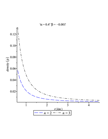
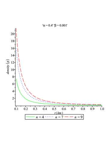
Figure 1: Variation of density $\rho$ against $r$ in the interior of the compact star for different dimensions: $4D$ and $5D$ in the left panel whereas $6D$, $9D$ and $11D$ in the right panel

3.1 The exterior spacetime and matching condition

The solution of the Einstein-Maxwell equation in higher dimensional spacetime for $r>R$ is given by the following Reissner-Nordström (RN) spacetime in higher dimension as

$$ds^{2}=-\left(1-\frac{\mu}{r^{n-1}}+\frac{Q^{2}}{r^{2(n-1)}}\right)dt^{2}+\left(1-\frac{\mu}{r^{n-1}}+\frac{Q^{2}}{r^{2(n-1)}}\right)^{-1}dr^{2}+r^{2}d\Omega^{2},$$ (31)

where $\mu$ is related to the mass $M$ as $\mu=\frac{16\pi GM}{n{\Omega}_{n}}$ and $Q$ is its charge. So our interior solution should match with Eq. (31) at the boundary $r=R$.

The continuity of the metric $e^{\nu}$ gives the constant $C_{2}$ as

$$C_{2}=\sqrt{\frac{1}{R^{2}}\left[1-\frac{\mu}{R^{n-1}}+\frac{Q^{2}}{R^{2(n-1)}}\right]}$$ (32)

and the continuity of $e^{\lambda}$ gives

$$Q^{2}=R^{2(n-1)}\left[\frac{(n-1)^{2}}{n}\frac{\alpha+1}{n+n\alpha-2\alpha}+\frac{16\pi\beta R^{2}}{(\alpha+1)(n+1)}-1+\frac{\mu}{R^{n-1}}\right].$$ (33)

The intensity of the electric field at the boundary can be obtained as

$$E(R)=\frac{Q(R)}{R^{n-2}}=R\sqrt{\frac{(n-1)^{2}}{n}\frac{\alpha+1}{n+n\alpha-2\alpha}+\frac{16\pi\beta R^{2}}{(\alpha+1)(n+1)}-1+\frac{\mu}{R^{n-1}}}.$$ (34)

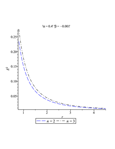
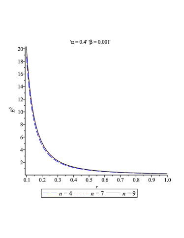
Figure 3: The Electric field are plotted against $r$ for different dimensions: $4D$ and $5D$ in the left panel whereas $6D$, $9D$ and $11D$ in the right panel

The profile of the electric field is shown in Fig. 3. The figure shows that $E^{2}$ is a monotonic decreasing function of $r$ which attains maximum value for $11D$ and minimum value for $4D$.

3.2 The Junction Condition

Here the metric coefficients are continuous at $r=R$, but that does not ensure that their derivatives are also continuous at the junction surface. In other words the affine connections may be discontinuous at the junction surface $r=R$. To take care of this we use the Darmois-Israel formation to determine the surface stresses at the junction boundary. The intrinsic surface stress energy tensor as given by Lancozs equations is as follows:

Obviously the metric coefficients are continuous at but it does not ensure that their derivatives are also continuous at the junction surface. In other words the affine connections may be discontinuous there. To take care of this let us use the Darmois-Israel formation to determine the surface stresses at the junction boundary. The intrinsic surface stress energy tensor $S_{ij}$ is given by Lancozs equations in the following form

$$S^{i}_{j}=-\frac{1}{8\pi}(\kappa^{i}_{j}-\delta^{i}_{j}\kappa^{k}_{k}).$$ (35)

The discontinuity in the second fundamental form is given by

$$\kappa_{ij}=K_{ij}^{+}-K_{ij}^{-},$$ (36)

where the second fundamental form is given by

$$K_{ij}^{\pm}=-n_{\nu}^{\pm}\left[\frac{\partial^{2}X_{\nu}}{\partial\xi^{i}\partial\xi^{j}}+\Gamma_{\alpha\beta}^{\nu}\frac{\partial X^{\alpha}}{\partial\xi^{i}}\frac{\partial X^{\beta}}{\partial\xi^{j}}\right]|_{S}.$$ (37)

Here $n_{\nu}^{\pm}$ are the unit normal vector defined by

$$n_{\nu}^{\pm}=\pm\left|g^{\alpha\beta}\frac{\partial f}{\partial X^{\alpha}}\frac{\partial f}{\partial X^{\beta}}\right|^{-\frac{1}{2}}\frac{\partial f}{\partial X^{\nu}},$$ (38)

with $n^{\nu}n_{\nu}=1$. Here $\xi^{i}$ is the intrinsic coordinate on the shell. $+$ and $-$ corresponds to exterior i.e, RN spacetime in higher dimension and interior (our) spacetime respectively.

Considering the spherical symmetry of the spacetime surface stress energy tensor can be written as $S^{i}_{j}=diag(-\Sigma,\mathcal{P},\mathcal{P},...,\mathcal{P})$ where $\Sigma$ and $\mathcal{P}$ are the surface energy density and surface pressure respectively and can be provided by

$$\Sigma=-\frac{n}{4\pi R}\sqrt{1-\frac{\mu}{R^{n-1}}+\frac{q^{2}}{R^{2(n-1)}}}+\frac{n}{4\pi R}\sqrt{\frac{(n-1)^{2}}{n}\frac{\alpha+1}{n+n\alpha-2\alpha}+\frac{16\pi\beta}{(1+\alpha)(n+1)}r^{2}},$$ (39)

$$\mathcal{P}=\frac{n-1}{4\pi R}\left(1+\frac{\mu}{2R^{n-1}}-\frac{q^{2}}{R^{2n-1}}\right)\sqrt{1+\frac{\mu}{2R^{n-1}}-\frac{q^{2}}{R^{2n-2}}}$$

$$-\frac{n}{4\pi R}\sqrt{\frac{(n-1)^{2}}{n}\frac{\alpha+1}{n+n\alpha-2\alpha}+\frac{16\pi\beta R^{2}}{(\alpha+1)(n+1)}}.$$ (40)

The mass of the thin shell can be obtained as

$$m_{s}=\frac{2\pi^{\frac{n+1}{2}}}{\Gamma\left(\frac{n+1}{2}\right)}R^{n}\Sigma.$$ (41)

Now using Eqs. (40) and (41) one can obtain the mass of the charged fluid sphere in terms of the mass of the thin shell as

$$\mu=R^{n-1}\left[1+\frac{q^{2}}{R^{2(n-1)}}-G^{2}+2BG-B^{2}\right],$$ (42)

where

$$G=\frac{2m_{s}\Gamma\left(\frac{n+1}{2}\right)}{nR^{n-1}\pi^{\frac{n-1}{2}}}$$

and

$$B=\sqrt{\frac{(n-1)^{2}}{n}\frac{\alpha+1}{n+n\alpha-2\alpha}+\frac{16\pi\beta R^{2}}{(\alpha+1)(n+1)}}.$$

4 Physical Analysis of the solutions

For a physically meaningful solution one must have pressure and density are decreasing function of $r$. For our model

$$\frac{dp}{dr}=-\frac{(n-1)^{2}}{n+\alpha(n-2)}\frac{\alpha}{4\pi r^{3}}<0,$$ (43)

$$\frac{d\rho}{dr}=-\frac{(n-1)^{2}}{n+\alpha(n-2)}\frac{1}{4\pi r^{3}}<0.$$ (44)

The above expression indicates that both $\rho$ and $p$ are monotonic decreasing function of $r$, i.e. the have maximum value at the center of the star and it decreases radially outwards. The constant of integration $\beta$ can be obtained by imposing the condition $p(r=R)=0$ as

$$\beta=\frac{\alpha(\alpha+1)(n-1)^{2}}{8\pi R^{2}(n+n\alpha-2\alpha)(n\alpha-\alpha-1)}.$$ (45)

The above equations consequently gives

$$R_{n}=\sqrt{\frac{\alpha(\alpha+1)(n-1)^{2}}{8\pi\beta(n+n\alpha-2\alpha)(n\alpha-\alpha-1)}},$$

where $n=D-2$, $D$ being the dimension of the spacetime. One can easily verify that

$$\frac{dp}{d\rho}=\alpha.$$

To satisfy the causality conditions one must have $0<\frac{dp}{d\rho}<1$ which implies $0<\alpha<1$. To find the radius of different dimensional charged star let us fix $\alpha=0.4$. From the expression of $R_{n}$ one can note that for $\alpha=0.4$, $n+(n-2)\alpha$ is always positive and $n\alpha-\alpha-1$ is negative for $n=2$ and $n=3$, i.e. for four and five dimensional spacetime. So we must have $\beta<0$ for $n=2$ and $n=3$. On the other hand $n\alpha-\alpha-1$ is positive for six dimensional onwards when $\alpha=0.4$. So we have to take positive beta for six dimensional onwards. So to find the radius of the charged star in different dimension we have choose $\alpha=0.4,\beta=-0.001$ for $4D$ and $5D$ spacetime and $\alpha=0.4,\beta=0.001$ for the spacetime onwards six dimension. The radius of the charged star in different dimension are shown in Table 1. From Fig. 2, we see that the radius of the star is found where the graphs of p(r) cut the r-axis and one can note that the radius of the charged star in $5D$ is greater than $4D$ for fixed values of $\alpha$ and $\beta$ mentioned in the figure. On the other hand the radius of the charged star decreases when the dimension increases, i.e. for for fixed values of $\alpha$ and $\beta$ mentioned in the figure the radius is maximum for $6D$ charged star and is minimum for $11D$ charged star.

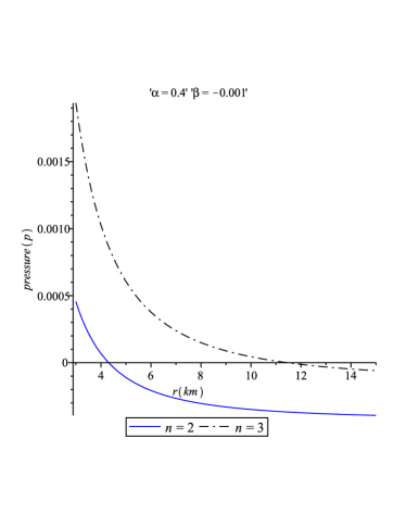
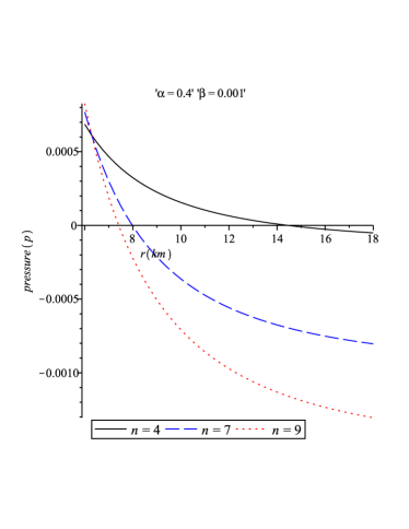
Figure 2: Radii of the stars are found where radial pressures cut $r$ axis for different dimensions: $4D$ and $5D$ in the left panel whereas $6D$, $9D$ and $11D$ in the right panel

The gravitational mass inside the charged sphere can be obtained as

$$m(r)=\int_{0}^{r}\frac{2\pi^{\frac{n+1}{2}}}{\Gamma\left(\frac{n+1}{2}\right)}r^{n}\left[\rho+\frac{E^{2}}{8\pi}\right]dr$$

$$~{}~{}~{}~{}~{}~{}~{}~{}~{}~{}~{}~{}~{}~{}~{}~{}~{}~{}~{}~{}~{}~{}~{}~{}~{}~{}~{}~{}~{}~{}~{}~{}~{}~{}~{}~{}~{}~{}~{}~{}~{}~{}~{}~{}~{}~{}~{}~{}~{}~{}~{}~{}~{}~{}~{}~{}=\frac{\pi^{\frac{n-1}{2}}}{4\Gamma\left(\frac{n+1}{2}\right)}\left[\frac{2n-(1+\alpha)}{2(n+n\alpha-2\alpha)}r^{n-1}-\frac{8n\pi\beta}{(1+\alpha)(n+1)}r^{n+1}\right].$$ (46)

The profile of the mass function for different dimensional compact stars are shown in Fig. 7. The figure indicates that $m(r)$ is a monotonic increasing function of r and $m(r)>0$ inside the charged fluid sphere. Moreover as $r\rightarrow 0$, $m(r)\rightarrow 0$, i.e. the mass function is regular at the center of the charged star.

The charged density can be obtained as

$$\sigma=\frac{\Gamma\left(\frac{n+1}{2}\right)}{2\pi^{\frac{n+1}{2}}}\frac{n-1}{r^{2}}\sqrt{\frac{(n-1)(1-\alpha)}{2(n+n\alpha-2\alpha)}}\sqrt{\frac{(n-1)^{2}}{n}\frac{\alpha+1}{n+n\alpha-2\alpha}+\frac{16\pi\beta}{(1+\alpha)(n+1)}r^{2}}.$$ (47)

The profile of the charged density is shown in Fig. 4. The figure indicates that it is a monotonic decreasing function of $r$ and its values increases as dimensions increases, i.e. the value of $\sigma$ is maximum for $11D$ and minimum for $4D$.

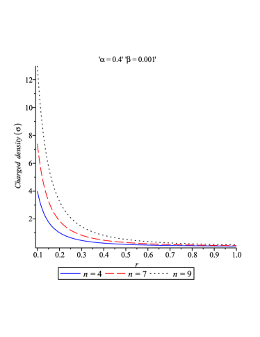
Figure 4: The charged density are plotted against $r$ for different dimensions: $4D$ and $5D$ in the left panel whereas $6D$, $9D$ and $11D$ in the right panel

4.1 Stability condition

To check the stability of our model under three different forces we consider the generalized TOV equation which is given by the equation verela

$$-\frac{M_{G}(\rho+p)}{r^{n-2}}e^{\frac{\lambda-\nu}{2}}-\frac{dp}{dr}+\sigma\frac{q}{r^{n-2}}e^{\frac{\lambda}{2}}=0,$$ (48)

where $M_{G}=M_{G}(r)$ is the effective gravitational mass inside a sphere of radius $r$ which can be derived from the equation

$$M_{G}(r)=\frac{1}{2}r^{n-2}e^{\frac{\nu-\lambda}{2}}\nu^{\prime}$$ (49)

named as Tolman-Whittaker formula. The above equation describes the equilibrium condition of the fluid sphere subject to gravitational,hydrostatics and electric forces. Eq. (44) can be modified in the form

$$F_{g}+F_{h}+F_{e}=0,$$ (50)

where

$$F_{g}=-\frac{\nu^{\prime}}{2}(\rho+p)=-\frac{1}{r}\left[\frac{\alpha+1}{n(1+\alpha)-2\alpha}\frac{(n-1)^{2}}{8\pi r^{2}}-\beta(n-1)\right],$$ (51)

$$F_{h}=-\frac{dp}{dr}=\frac{(n-1)^{2}}{n+\alpha(n-2)}\frac{\alpha}{4\pi r^{3}},$$ (52)

$$F_{e}=\sigma\frac{q}{r^{n-2}}e^{\frac{\lambda}{2}}.$$ (53)

The profiles of $F_{g},~{}F_{h}~{}F_{e}$ has shown in Fig. 5 for different dimensional charged fluid sphere. The figure shows that for our model the gravitational force $(F_{g})$ is counterbalanced by the combined effects of hydrostatic $(F_{h})$ and electric forces $(F_{e})$ and thus helps to keep the model in static equilibrium.

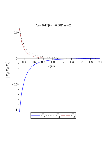
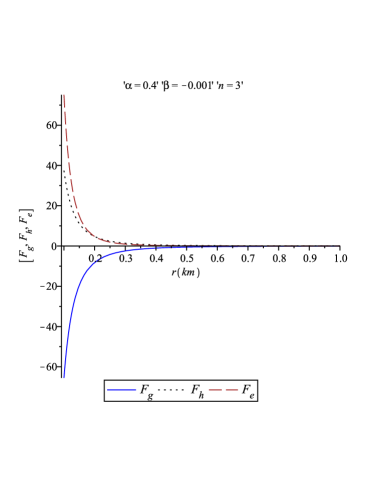
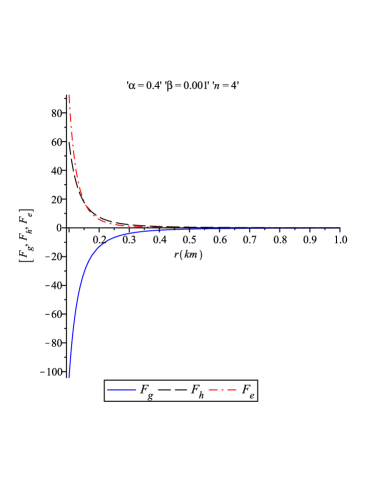
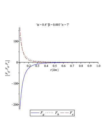
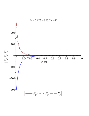
Figure 5: The three different forces, namely, gravitational forces $(F_{g})$, hydrostatic forces $(F_{h})$ and electric forces $(F_{e})$ are plotted against ‘r (km)’ for $4D$ (upper left), $5D$ (upper right), $6D$ (middle left), $9D$ (middle right) and $11D$ (lower)

4.2 Energy Conditions

The isotropic charged perfect fluid sphere will satisfy the Null energy condition (NEC), Weak energy condition (WEC) and Strong energy condition if the following inequalities hold simultaneously inside the fluid sphere:

$$\rho+\frac{E^{2}}{8\pi}\geq 0,$$ (54)

$$\rho+p\geq 0,$$ (55)

$$\rho+p+\frac{E^{2}}{4\pi}\geq 0,$$ (56)

$$\rho+3p+\frac{E^{2}}{4\pi}\geq 0.$$ (57)

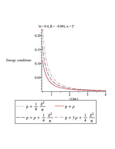
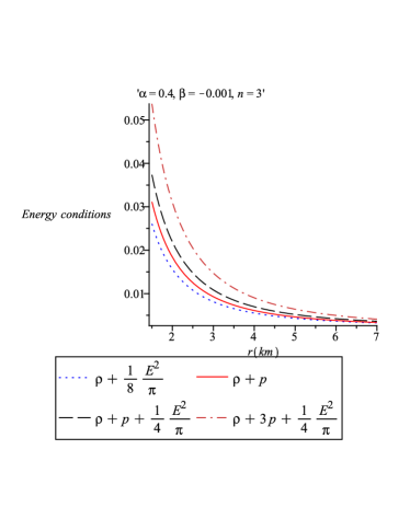
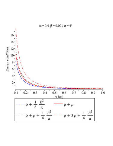
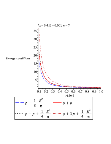
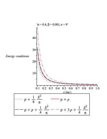
Figure 6: The energy conditions are plotted against $r$ for $4D$ (upper left), $5D$ (upper right), $6D$ (middle left), $9D$ (middle right) and $11D$ (lower)

The graphs of the Energy conditions corresponding to different dimensions are shown in Fig. 6, which indicates that all the Energy conditions are satisfied by proposed model of charged fluid sphere in different dimensional spacetime.

4.3 Compactness and Redshift

We have already obtained the gravitational mass $m(r)$ of the system in Eq. (30). Using this, one can easily find the compactness factor and redshift of the star are respectively as

$$u(r)=\frac{m(r)}{r},$$ (58)

$$z_{s}=(1-2u)^{-1/2}-1.$$ (59)

The graphs of compactness factor and surface redshift corresponding to different dimensions are given in Figs. 7 and 8.

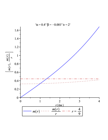
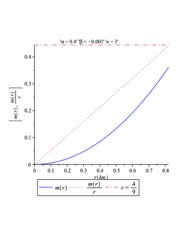
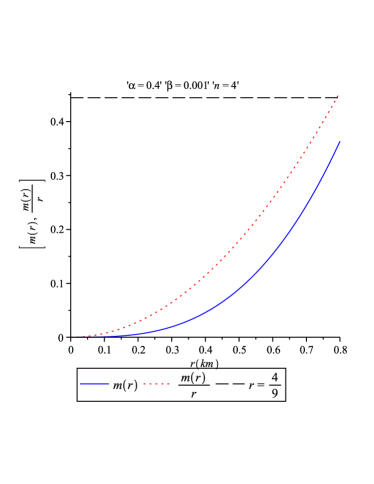
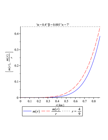
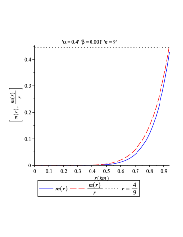
Figure 7: The mass and compactness factor are plotted against $r$ for $4D$ (upper left), $5D$ (upper right), $6D$ (middle left), $9D$ (middle right) and $11D$ (lower)

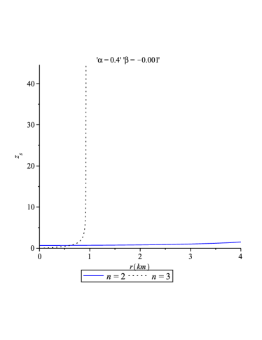
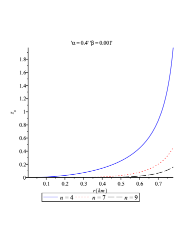
Figure 8: The redshift of the star are plotted against $r$ for different dimensions: $4D$ and $5D$ in the left panel whereas $6D$, $9D$ and $11D$ in the right panel

5 Discussion and Conclusion

In the present paper we have obtained a new set of interior solutions for charged isotropic stars admitting conformal motion in higher dimensional spacetime. Several interesting features have been observed which are as follows:

(1) The obtained solutions are well behaved for $r>0$. The matter-energy density $\rho$, fluid pressure p and electric field intensity $E$ are all monotonically decreasing functions of radial coordinate $r$. All the physical quantities are mostly regular throughout the stellar configuration.

(2) The mass of the star has been proposed (see Eq. (43)) in terms of the thin shell mass.

(3) Various physical properties like the compactness factor and surface redshift are studied not only in the standard four dimensional spacetime but also in higher dimensions. We notice that the surface redshift of the star does not exist for the spacetime related to sixth dimensions (see Table 1).

(4) We have estimated the radii of the star in different dimensions by means of plots (see Table 1). The radii are found out through the technique where the radial pressures meet the radial coordinate $r$. We note that for negative value of $\beta$ radial pressures vanish at the boundary for $4D$ and $5D$ cases and for positive value of $\beta$ radial pressures vanish at the boundary beyond five dimensions. The radii of the star are found to be a few kilometers only for different dimensions and masses of the stars are comparable with the mass of the sun. This data clearly indicates that the model represents a compact star. Plugging the numerical values of the physical constants $G$ and $c$ in the relevant expressions, we have found out mass of the star as $1.204~{}M_{\odot}$ and the surface density as $3.49\times 10^{15}$ (gm/cc) in four dimensional background. We observe that this data as obtained in the Table 1 is quite close to $SAX~{}J1808.4-3658~{}(SS2)$ its mass being $1.323$ $M_{\odot}$.

Table 1: Values of the physical parameters for the strange star candidate $SAX~{}J1808.4-3658~{}(SS2)$ related to different dimensions. Here the computations are shown up to the Buchdahl limit with radius $r=0.84$ km

Dimension	$\beta$	Radius $(p_{r}=0)$	Mass	Mass	$\rho_{s}$	$Z_{s}$
		(km)	(km)	($M_{\odot}$)	(gm/cc)
4	$-0.001$	4.14	1.776	1.204	$3.49\times 10^{15}$	1.637
5	$-0.001$	11	0.3803043117∗	0.2578334317∗	$92.61864817\times 10^{15}$∗	2.252767160∗
6	0.001	14	0.4205932803∗	0.2851479866∗	$139.1248886\times 10^{15}$∗	does not exist∗
9	0.001	7.8	0.3130416663∗	0.2122316382∗	$298.2815551\times 10^{15}$∗	0.98160610∗
11	0.001	7.1	0.1743244558∗	0.1181860717	$404.9245698\times 10^{15}$∗	0.307505974∗

(5) The most important result we obtain is that the model satisfies the Buchdahl inequality i.e. $\frac{m(R)}{R}<\frac{4}{9}$ for four dimensional spacetime only. For the spacetime more than four, Buchdahl inequality does not hold good up to the radius of the star in the range 4-11 km for which $p_{r}(r=R)=0$. However, a thourough investigation shows that up to the radius $0.84$ km (approx) Buchdahl inequality holds good for dimension more than four dimensions also. Along with this also all the other physical characteristics are well behaved and the energy conditions are satisfied up to radius $0.84$ km (see Table 1).

In this regard, specifically we would like to mention that in one of our previous work Bhar2015b we obtained the radius from the plot within 1 km and, therefore, the above feature could not been verified. Now, it can be seen that if we go over 1 km then Buchdahl inequality does not hold good in the work of Bhar et al. Bhar2015b and this new property has been overlooked in previous all studies. As a summary, it reveals that though the stars under the present investigation have radius within the range 4-11 km, but they satisfy Buchdahl inequality within $0.84$ km only.

(6) We have analyzed the TOV equations for different dimensions which indicate that the gravitational force of the star is balanced by the combined effect of the hydrostatic and electric forces. This implies that the system is in static equilibrium under these three forces. Thus our study reveals that up to the radius for which Buchdahl inequality holds good, the compact stars are well behaved in higher dimensional spacetime.

Hence on a primary stage, unlike Bhar et al. Bhar2015b and Ghosh et al. Ghosh2015 , it seems that compact stars do exist even in higher dimensional spacetime as proposed in the current paper. However, before accepting this theoretical result as fact other type of investigations with different propositions are extmremly needed to perform.

References

- (1) J.H. Schwarz, Superstings, World Scientific, Singapore (1985)
- (2) S. Weinberg, Strings and Superstrings, World Scientific, Singapore (1986)
- (3) M.J. Duff, J.T. Liu, R. Minasian, Nucl. Phys. B 452, 261 (1995)
- (4) J. Polchinski, String Theory (Cambridge, 1998)
- (5) S. Hellerman, I. Swanson, J. High Energy Phys. 0709, 096 (2007)
- (6) O. Aharony, E. Silverstein, Phys. Rev. D 75, 046003 (2007)
- (7) R. Emparan, H.S. Reall, Liv. Rev. Relativ. 11, 6 (2008)
- (8) A. Pradhan, G.S. Khadekar, M.K. Mishra and S. Kumbhare, Chin. Phys. Letter. 24, 3013 (2007)
- (9) G.S. Khadekar and S. Kumbhare, Clifford Analysis, Clifford Algebras and Their Applications 3, 307 (2014)
- (10) R. Stettner, Ann. Phys. 80, 212 (1973)
- (11) A. Krasinski, Inhomogeneous cosmological models, Cambridge University Press (1997).
- (12) R. Sharma, S. Mukherjee and S.D. Maharaj, Gen. Relativ. Gravit. 33, 999 (2001)
- (13) P.S. Joshi, Global aspects in gravitation and cosmology, Oxford, Clarendon Press (1993)
- (14) B.V. Ivanov, Phys. Rev. D 65, 104001 (2002)
- (15) P.M. Takisa, S.D. Maharaj, Astrophys. Space Sci. 343, 569 (2013)
- (16) S. Thirukkanesh, S. Maharaj, Class. Quantum Gravit. 25, 235001 (2008)
- (17) V. Varela, F. Rahaman, S. Ray, K. Chakraborty, M. Kalam, Phys. Rev. D 82, 044052 (2010)
- (18) F. Rahaman, S. Ray, A.K. Jafry, K. Chakraborty, Phys. Rev. D 82, 104055 (2010)
- (19) K.D. Krori, J. Barua, J. Phys. A 8, 508 (1975)
- (20) C.G. Böhmer, T. Harko, F.S.N. Lobo, Phys. Rev. D 76, 084014 (2007)
- (21) C.G. Böhmer, T. Harko, F.S.N. Lobo, Class. Quant. Gravit. 25, 075016 (2008)
- (22) K. Krori, P. Borgohain, K. Das, A. Sarma, Can. J. Phys. 64, 887 (1986)
- (23) K. Krori, P. Borgohain, K. Das, A. Sarma, Can. J. Phys. 64, 882 (1986)
- (24) R. Maartens, M. Maharaj, J. Math. Phys. 31, 151 (1990)
- (25) L. Herrera and J. Ponce de León, J. Math. Phys. 26, 778 (1985)
- (26) F. Rahaman, M. Jamil, R. Sharma, K. Chakraborty, Astrophys. Space Sci. 330, 249 (2010)
- (27) A.A. Usmani, F. Rahaman, S. Ray, K.K. Nandi, P.K.F. Kuhfittig, Sk.A. Rakib, Z. Hasan, Phys. Lett. B 701, 388 (2011)
- (28) P. Bhar, Astrophys. Space Sci. 354, 457 (2014)
- (29) F. Rahaman, M. Jamil, M. Kalam, K. Chakraborty, A. Ghosh, Astrophys. space Sci. 137, 325 (2010)
- (30) L. Herrera, J. Ponce de León, J. Math. Phys. 26, 2302 (1985)
- (31) L. Herrera, J. Ponce de León, J. Math. Phys. 26, 2018 (1985)
- (32) M. Esculpi, E. Aloma, Eur. Phys. J. C 67, 521 (2010)
- (33) S. Ray, Gen. Relativ. Gravit. 36, 1451 (2004)
- (34) S. Ray, B. Das, Gravit. Cosmol. 13, 224 (2007)
- (35) M.K. Mak and T. Harko, Int. J. Mod. Phys. D 13, 149 (2004)
- (36) T. Harko and M.K. Mak, Ann Phys. 319, 471 (2005)
- (37) P. Bhar, Eur. Phys. J. C 75, 123 (2015)
- (38) P.C. Vaidya, R. Titekar, J. Astrophy. Astron. 3, 325 (1982)
- (39) W. Israel, Nuo. Cim. B 44, 1 (1966)
- (40) W. Israel, Nuo. Cim. B 48, 463 (1967)
- (41) H.A. Buchdahl, Phy. Rev. 116, 1027 (1959)
- (42) K. Nozari, S.H. Mehdipour, JHEP 0903, 061 (2009)
- (43) S.H. Mehdipour, Eur. Phys. J. Plus 127, 80 (2012)
- (44) P. Bhar, F. Rahaman, S. Ray, V. Chatterjee, Eur. Phys. J. C 75, 190 (2015)
- (45) S. Ghosh, F. Rahaman, B.K. Guha, S. Ray, arXiv:1511.05417