Failure of classical traffic flow theories:
Stochastic highway capacity and automatic driving

Abstract

In a mini-review [Physica A 392 (2013) 5261–5282] it has been shown that classical traffic flow theories and models failed to explain empirical traffic breakdown – a phase transition from metastable free flow to synchronized flow at highway bottlenecks. The main objective of this mini-review is to study the consequence of this failure of classical traffic-flow theories for an analysis of empirical stochastic highway capacity as well as for the effect of automatic driving vehicles and cooperative driving on traffic flow. To reach this goal, we show a deep connection between the understanding of empirical stochastic highway capacity and a reliable analysis of automatic driving vehicles in traffic flow. With the use of simulations in the framework of three-phase traffic theory, a probabilistic analysis of the effect of automatic driving vehicles on a mixture traffic flow consisting of a random distribution of automatic driving and manual driving vehicles has been made. We have found that the parameters of automatic driving vehicles can either decrease or increase the probability of traffic breakdown. The increase in the probability of traffic breakdown, i.e., the deterioration of the performance of the traffic system can occur already at a small percentage (about 5$\%$) of automatic driving vehicles. The increase in the probability of traffic breakdown through automatic driving vehicles can be realized, even if any platoon of automatic driving vehicles satisfies condition for string stability.

1 Introduction. The reason for paradigm shift in traffic and transportation science

A current effort of many car-developing companies is devoted to the development of automatic driving vehicles. It is assumed that the future vehicular traffic consisting of human driving and automatic driving vehicles should considerably enhance highway capacity.

Highway capacity is limited by traffic breakdown, i.e., a transition from free flow to congested traffic [1, 2, 3, 4, 5, 6, 7, 8, 9, 10, 11, 12, 13, 14, 15, 16, 17]. Traffic breakdown with resulting traffic congestion occurs usually at a road bottleneck (see, e.g., [1, 2, 3, 4, 5, 6, 7, 8, 9, 10, 11, 12, 13, 14, 15],

[16, 17, 18, 19, 20, 21, 22, 23, 24, 25, 26, 27, 28, 29, 30, 31, 32, 33, 34, 35],

[36, 37, 38, 39, 40, 41, 42, 43, 44, 45, 46, 47, 48, 49, 50, 51, 52, 53],

[54, 55, 56, 57, 58, 59, 60, 61, 62, 63, 64, 65, 66, 67, 68, 69, 70],

[71, 72, 73, 74, 75, 76, 77, 78, 79, 80, 81, 82, 83, 84, 85, 86, 87],

[88, 89, 90, 91, 92, 93, 94, 95, 96, 97, 98, 99, 100, 101, 102, 103, 104, 105, 106, 107, 108, 109],

[110, 111, 112, 113, 114, 115, 116, 117, 118, 119, 120, 121, 122, 123, 124, 125, 126, 127, 128, 129, 130],

[131, 132, 133, 134, 135, 136, 137, 138, 139, 140, 141, 142, 143, 144, 145, 146, 147, 148, 149, 150, 151, 152] and references in reviews, books, and conference proceedings

[153, 154, 155],  [156, 157, 158, 159, 160, 161, 162, 163, 164, 165, 166, 167, 168, 169, 170, 171],

[172, 173, 174, 175, 176, 177, 178, 179, 180, 181, 182, 183, 184],

[185, 186, 187, 188, 189, 190, 191, 192, 193, 194, 195, 196, 197, 198, 199, 200, 201, 202, 203, 204, 205]). Road bottlenecks are caused, for example, by road works, on- and off-ramps, road gradients, reduction of lane number (see, e.g., [2, 3, 4]), slow moving vehicles (called $``$moving bottlenecks”) [206, 207, 208, 209, 210, 211, 212, 213, 214, 215]. Therefore, to understand the nature of highway capacity of real traffic, empirical features of traffic breakdown at a bottleneck should be known.

1.1 Achievements of empirical study of traffic breakdown

Beginning from the classical work by Greenshields [1], a great effort has been made to understand the empirical features of traffic breakdown (see, e.g., [2, 3, 4, 5, 6, 7, 8, 9, 10],  [11, 12, 13, 14, 15, 16, 17]). Traffic breakdown at a highway bottleneck is a local phase transition from free flow (F) to congested traffic whose downstream front is usually fixed at the bottleneck location (Fig. 1 (a, b)) [2, 3, 4, 5, 6, 7, 8, 9, 10, 11, 12, 13, 14, 15, 16, 17]. In three-phase traffic theory, such congested traffic is called synchronized flow (S) [200, 201]. In other words, using the terminology of the three-phase traffic theory, traffic breakdown is a transition from free flow to synchronized flow (called F$\rightarrow$S transition) [200, 201]. However, it should be emphasized that as long as features of synchronized flow are not discussed (this discussion will be done in Sec. 1.3), the term synchronized flow is nothing more as only the definition of congested traffic whose downstream front is fixed at the bottleneck.

During traffic breakdown vehicle speed sharply decreases (Fig. 1 (c)). For this reason, traffic breakdown is also called speed drop or speed breakdown [2, 3, 4, 5, 6, 7, 8, 9, 10, 11],  [12, 13, 14, 15, 16, 17]. In contrast, after traffic breakdown has occurred the flow rate can remain as large as in an initial free flow (Fig. 1 (d)) [5, 6, 7, 8, 9, 10, 11, 16, 17]. In the review article, the flow rate in free flow at the bottleneck is denoted by $q=q_{\rm sum}$.

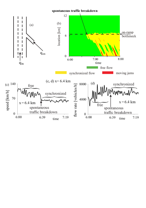
Figure 1: Empirical features of spontaneous traffic breakdown (spontaneous F$\rightarrow$S transition) at on-ramp bottleneck. Real field traffic data measured on three-lane freeway A5-South in Germany on April 15, 1996: (a) Schema of three-lane freeway with on-ramp bottleneck. (b) Speed data measured with road detectors installed along road section; data is presented in space and time with averaging method described in Sec. C.2 of [149]. (c, d) 1-min average data for speed (c) and flow rate (d) as time functions measured at location $x=$ 6.4 km. Empirical results are qualitatively the same as those found from studies of real field traffic data measured in different countries [2, 3, 4, 5, 6, 7, 8, 9, 10, 11, 12, 13, 14, 15, 16, 17]. Free – free flow, synchronized – synchronized flow.

In 1995, Elefteriadou et al. [9, 16, 17] found that traffic breakdown at a highway bottleneck has a stochastic (probabilistic) behavior. This means the following: At a given flow rate $q_{\rm sum}$ in free flow at the bottleneck traffic breakdown can occur but it should not necessarily occur. Thus on one day traffic breakdown occurs, however, on another day at the same flow rate $q_{\rm sum}$ traffic breakdown is not observed. Studying the probability for the probabilistic breakdown phenomenon at a freeway bottleneck, in 1998 Persaud et al. [10] discovered that the probability $P^{\rm(B)}(q_{\rm sum})$ of traffic breakdown is an increasing function of the flow rate $q_{\rm sum}$ in free flow at the bottleneck. The empirical result of Persaud et al. [10] has also been found for freeways in the USA by Lorenz and Elefteriadou [11] as well as for German freeways by Brilon et al. [12, 13, 14, 15].

Traffic parameters, like weather, percentage of long vehicles in traffic flow, shares of aggressive and timid drivers are stochastic time-functions. Thus it is generally assumed that the stochastic nature of real traffic breakdown might be explained by classical traffic flow theories, in which stochastic traffic parameters should be taken into account (see, e.g. [5, 6, 7, 8, 9, 10, 11, 16, 17, 181] and references there).

• In contrast with this general accepted assumption [5, 6, 7, 8, 9, 10, 11, 16, 17, 181], in Sec. 1.3 we will explain that the sole knowledge of the above-mentioned features of empirical traffic breakdown at highway bottlenecks and highway capacity revealed and reviewed in [1, 2, 3, 4, 5, 6, 7, 8, 9],  [10, 11, 12, 13, 14, 15, 16, 17] is not sufficient to disclose the physical nature of traffic breakdown and associated stochastic highway capacity. Indeed, we will find that empirical stochastic highway capacity exhibits the nucleation nature that contradicts basic results of classical traffic flow theories. In particular, in Sec. 3 we will show that the classical understanding of stochastic highway capacity that is generally accepted [5, 6, 7, 8, 9, 10, 11, 16, 17] is invalid for real traffic.

1.2 Basic assumption of three-phase traffic theory

As emphasized in Sec. 1.1, real traffic breakdown at a road bottleneck is an F$\rightarrow$S transition. To explain features of empirical traffic breakdown at highway bottlenecks, in three-phase traffic theory introduced by the author in 1996-2002 (three-phase theory, for short) has been assumed that traffic breakdown is the F$\rightarrow$S transition at the bottleneck that occurs in metastable free flow [200, 201, 216, 217, 218, 219, 220, 221, 222, 223, 224, 225, 226, 227, 228, 229, 230]. Thus in the three-phase theory the term traffic breakdown is a synonym of the term F$\rightarrow$S transition occurring in metastable free flow at the bottleneck.

The term $``$metastable free flow with respect to the F$\rightarrow$S transition at a bottleneck” means that a small enough disturbance (speed, density, and/or flow rate) in free flow at the bottleneck decays. Therefore, in this case free flow persists at the bottleneck over time. However, when a disturbance of a large enough amplitude appears in free flow in a neighborhood of the bottleneck, an F$\rightarrow$S transition occurs at the bottleneck. In accordance with other metastable systems of natural science [231, 232, 233, 234, 235],  [236, 237, 238, 239, 240, 241, 242] such a local disturbance in free traffic flow can be called a nucleus for traffic breakdown (F$\rightarrow$S transition) at a bottleneck.

• A nucleus for traffic breakdown (F$\rightarrow$S transition) at a bottleneck is a time-limited local disturbance in free flow that does lead to traffic breakdown at the bottleneck.

This means that traffic breakdown at the bottleneck exhibits the nucleation nature: If the nucleus for traffic breakdown occurs in free flow at the bottleneck, traffic breakdown does occurs. In contrast, as long as no nucleus appears, no traffic breakdown occurs in a metastable state of free flow.

• The basic assumption of the three-phase theory is that traffic breakdown at a bottleneck is the F$\rightarrow$S transition that exhibits the nucleation nature.

The basic assumption of the three-phase theory can mathematically be formulated as follows [200, 201, 216, 217, 218, 219, 220, 221],  [224, 225, 226, 227, 228, 229, 230]:

$$P^{\rm(B)}(q_{\rm sum})=P^{\rm(B)}_{\rm nucleus}(q_{\rm sum}),$$ (1)

where $P^{\rm(B)}(q_{\rm sum})$ is a flow rate dependence of the probability that during a given time interval $T_{\rm ob}$ traffic breakdown (F$\rightarrow$S transition) occurs in free flow at the bottleneck, $P^{\rm(B)}_{\rm nucleus}(q_{\rm sum})$ is the flow-rate dependence of the probability that during the time interval $T_{\rm ob}$ a nucleus for traffic breakdown occurs spontaneously in this free flow at the bottleneck. A mathematical nucleation theory of traffic breakdown can be found in [243, 244, 245].

1.3 Empirical proof of nucleation nature of traffic breakdown

In real traffic flow, there always different drivers and vehicles. Therefore, to perform a clear empirical proof of the nucleation nature of traffic breakdown that is independent of differences in vehicle and driver characteristics in free flow, we distinguish between empirical spontaneous traffic breakdown (Fig. 1) and empirical induced traffic breakdown (Fig. 2) [200, 201, 204, 205]:

1. Empirical spontaneous traffic breakdown is defined as follows. If before traffic breakdown occurs at the bottleneck, there is free flow at the bottleneck as well as upstream and downstream in a neighborhood of the bottleneck, then traffic breakdown at the bottleneck is called spontaneous traffic breakdown (Fig. 1).

2. Empirical induced traffic breakdown at the bottleneck is traffic breakdown induced by the propagation of a spatiotemporal congested traffic pattern. This congested pattern has occurred earlier than the time instant of traffic breakdown at the bottleneck and at a different road location (for example at a downstream bottleneck) than the bottleneck location (Fig. 2).

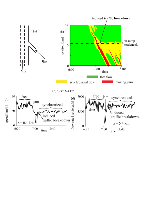
Figure 2: Empirical features of induced traffic breakdown (induced F$\rightarrow$S transition) at on-ramp bottleneck. Real field traffic data measured on three-lane freeway A5-South in Germany on March 22, 2001: (a) Schema of three-lane freeway with on-ramp bottleneck that is the same as that in Fig. 1 (a). (b) Speed data measured with road detectors installed along road section; data is presented in space and time with averaging method described in Sec. C.2 of [149]. (c, d) 1-min average data for speed (c) and flow rate (d) as time functions measured at location $x=$ 6.4 km. Free – free flow, synchronized – synchronized flow, jam – wide moving jam.

In contrast with Fig. 1 (b–d) in which synchronized flow has spontaneously emerged at the on-ramp bottleneck, in Fig. 2 (b) synchronized flow has been induced at the on-ramp bottleneck due to the propagation of a wide moving jam through the bottleneck. In both cases (Figs. 1 (c, d) and 2 (c, d)), synchronized flow resulting from the breakdown at the bottleneck is self-maintained under free flow conditions downstream of the bottleneck. Empirical features of synchronized flow resulting from the induced breakdown (at $t>$ 7:07 in Fig. 2 (b–d)) are qualitatively identical to those found in synchronized flow resulting from empirical spontaneous traffic breakdown (Fig. 1 (b–d)). This means that after the breakdown has occurred, characteristics of synchronized flow that has been formed at the bottleneck do not depend on whether synchronized flow has occurred due to empirical spontaneous breakdown (Fig. 1 (c, d)) or due to empirical induced breakdown (Fig. 2 (c, d)). In particular, as in the case of empirical spontaneous breakdown, in the case of empirical induced traffic breakdown the flow rate in synchronized flow resulting from the breakdown can be as high as the flow rate in free flow just before the breakdown has occurred (location $x=$ 6.4 km in Figs. 1 (d) and 2 (d)); this is in contrast with the wide moving jam within which the flow rate is very small [200, 201]

In [200, 201, 246], it has been shown that in real field traffic data there can be found many different scenarios of empirical spontaneous and induced traffic breakdowns. All these scenarios show qualitatively the same nucleation nature of traffic breakdown.

• The terms empirical spontaneous traffic breakdown and empirical induced traffic breakdown at a bottleneck distinguish different sources of a nucleus that occurrence leads to traffic breakdown [200, 201, 216, 217, 218, 219, 220, 221, 222],

  [223, 224, 225, 226, 227, 228, 229, 230, 246]:

• As found in [246], the source of empirical spontaneous breakdown is usually one of the waves in free flow that reaches a permanent speed disturbance localized at a highway bottleneck. The source of empirical induced breakdown is a localized moving congested pattern that reaches the location of the bottleneck (in Fig. 2 (b), this localized pattern is a wide moving jam).

• The empirical evidence of induced F$\rightarrow$S transition is the empirical proof of the metastability of free flow with respect to traffic breakdown (F$\rightarrow$S transition) (Fig. 2 (b–d)). This empirical proof is independent on the degree of the heterogeneity of real vehicular traffic.

Indeed, the empirical evidence of induced traffic breakdown is the empirical proof that at a given flow rate at a bottleneck there can be one of two different traffic states at the bottleneck: (i) A traffic state related to free flow and (ii) a congested traffic state labeled as synchronized flow in Fig. 2(b). Due to the upstream propagation of a localized congested pattern, a transition from the state of free flow to the state of synchronized flow, i.e., traffic breakdown is induced. A more detailed discussion of the empirical proof of the nucleation nature of real traffic breakdown can be found in [246].

We can make the following conclusions:

• The nucleation nature of real traffic breakdown at road bottlenecks is the fundamental empirical result that changes basically the theoretical fundamentals of transportation science.

• For this reason, the empirical metastability of free flow with respect to the F$\rightarrow$S transition (traffic breakdown) at a highway bottleneck can be considered the empirical fundament of transportation science.

Therefore, rather than features of traffic congested patterns resulting from traffic breakdown, in this min-review we analyze the impact of the nucleation nature of real traffic breakdown on stochastic highway capacity and on characteristics of intelligent transportation systems (ITS).

1.4 Failure of applications of classical traffic and transportation theories for analysis of intelligent transportation systems (ITS) and traffic network optimization

Generally accepted classical traffic and transportation theories have had a great impact on the understanding of many empirical traffic phenomena. In particular, the Lighthill-Whitham-Richards (LWR) model [247, 248] and associated kinetic macroscopic traffic flow models as well as in traffic flow models of the General Motors (GM) model class, diverse driver behavioral characteristics related to real traffic have been discovered and incorporated [153, 156, 157, 158, 159, 160, 161],

[162, 163, 164, 165, 166, 168, 170, 171],

[172, 173, 174, 175, 176, 179, 180, 181].

However, as explained in [204, 205], the classical traffic and transportation theories have nevertheless failed by their applications in the real world. Even several decades of a very intensive effort to improve and validate network optimization and control models based on the classical traffic and transportation theories had have no success. Indeed, there can be found no examples where on-line implementations of the network optimization models based on these classical traffic and transportation theories could reduce congestion in real traffic and transportation networks.

This failure of classical traffic and transportation theories is explained as follows [204, 205]:

• The LWR model [247, 248] cannot show the nucleation nature of traffic breakdown at highway bottlenecks. For this reason, the LWR theory as well as further theoretical approaches based on the LWR theory, like Daganzo’s cell transmission model (CTM) [249, 250], N-curves [209, 128, 251], and a macroscopic fundamental diagram (MFD) [252, 253] (see also references in recent publications [254, 255, 256, 257, 258]) are inconsistent with the nucleation nature of real traffic breakdown at road bottlenecks. Applications of these approaches for an analysis of the effect of ITS on traffic flow, which are widely used by many researchers, do lead to invalid (and sometimes incorrect) conclusions about the ITS performance in real traffic.

• In traffic flow models belonging to the GM model class introduced by Herman, Gazis, Montroll, Potts, Rothery, and Chandler [259, 260, 261, 262], traffic breakdown is associated with the classical traffic flow instability caused by a time delay in vehicle deceleration due to driver reaction time. As has been firstly shown by Kerner and Konhäuser [263, 264], the classical traffic flow instability revealed by Herman, Gazis, Montroll, Potts, Rothery, and Chandler [259, 260, 261, 262] leads to a phase transition from free flow (F) to a moving jam(s) (J) (called F$\rightarrow$J transition). The classical traffic flow instability has been incorporated in a huge number of traffic flow models; examples are the well-known optimal velocity (OV) model by Newell [265, 266, 267], a stochastic version of Newell’s model [268], the Nagel-Schreckenberg (NaSch) cellular automaton (CA) model [269, 270], Gipps model [271, 272], a stochastic model by Krauß et al. [273, 274], Payne’s macroscopic model [275, 276], Whitham’s model [277], Wiedemann’s model [163], the OV model by Bando et al. [278, 279, 280], Treiber’s intelligent driver model [281], the Aw-Rascle macroscopic model [282], a full velocity difference OV model by Jiang et al. [283], a lattice model by Nagatani [284, 285], and a huge number of other traffic flow models. There is a huge number of other traffic flow models belonging to the GM model; some of the models of the GM model class as well as results of their analysis can be found, for example, in

  [213, 214, 286, 287, 288, 289, 290, 291, 292, 293, 294, 295, 296, 297, 298, 299, 300, 301],

  [302, 303, 304, 305, 306, 307, 308, 309, 310, 311, 312, 313, 314, 315, 316, 317, 318, 319, 320, 321, 322, 323, 324],

  [325, 326, 327, 328, 329, 330, 331, 332, 333, 334, 335, 336, 337, 338, 339, 340, 341, 342, 343, 344, 345, 346],

  [347, 348, 349, 350, 351, 352, 353, 354, 355, 356, 357, 358, 359, 360, 361, 362, 363, 364, 365, 366, 367],

  [368, 369, 370, 371, 372, 373, 374, 375, 376, 377, 378]

  and reviews [159, 160, 161, 165, 166, 168, 170, 171, 172, 175, 177, 179, 180, 181, 379]). An F$\rightarrow$J transition exhibits a nucleation nature; however, the nucleation nature of the F$\rightarrow$J transition contradicts to the nucleation nature of empirical traffic breakdown: Rather than an F$\rightarrow$J transition, real traffic breakdown is the F$\rightarrow$S transition.

• Classical models for dynamic traffic assignment, control and optimization of traffic and transportation networks, for example, which are based on Wardrop’s user equilibrium (UE) and system optimum (SO) principles [380] (see, e.g., [258, 381, 382, 383, 384, 385, 386, 387, 388, 389, 390, 391, 392, 393, 394, 395, 396, 397, 398],

  [399, 400, 401, 402, 403, 404, 405, 406, 407, 408, 409, 410],

  [411, 412, 413, 414, 415, 416, 417, 418, 419, 420, 421, 422, 423, 424, 425, 426, 427, 428, 429, 430, 431, 432]

  and references in reviews [433, 434, 435, 436, 437]), failed due to the metastability of empirical free flow with respect to an F$\rightarrow$S transition at a network bottleneck. This is explained as follows [204]. The objective of these and other classical approaches to dynamic traffic assignment, control, and optimization of a traffic network is the minimization of travel times (and/or other $``$travel costs”) in the network. However, this leads to a considerable increase in the probability of traffic breakdown (F$\rightarrow$S transition) on some of the network links [204, 438]. The increase in the breakdown probability results in the deterioration of the performance of the traffic system.

Thus the classical traffic and transportation theories are not consistent with the nucleation nature of empirical traffic breakdown at a highway bottleneck. This is due to the fact that the nucleation nature of empirical traffic breakdown have been understood only during last 20 years. In contrast, the classical theoretical works, in particular, made by Wardrop [380], Lighthill, Whitham, and Richards [247, 248], Herman, Gazis, Montroll, Potts, Rothery, and Chandler [259, 260, 261, 262], Newell [265, 266], Kometani and Sasaki [439, 440, 441], Prigogine [442], Reuschel [443], and Pipes [444] that are the basic for the generally accepted fundamentals and methodologies of traffic and transportation theory have been introduced in the 1950s–1960s. These and other scientists whose ideas led to the classical fundamentals and methodologies of traffic and transportation theory could not know the nucleation nature of real traffic breakdown at road bottlenecks.

Because none of the classical traffic flow models can show the F$\rightarrow$S transition in metastable free flow at the bottleneck, as already emphasized in [204], the application of these classical models for an analysis of the effect of ITS on traffic flow, which is generally accepted by traffic and transportation researchers, do lead to invalid (and sometimes incorrect) conclusions about the ITS performance in real traffic. This criticism is related to all ITS that affect traffic flow, for example, on-ramp metering (see, e.g., [445, 446, 447, 448, 449, 450, 451, 452]), variable speed limit control (see, e.g., [452, 453, 454, 455, 456, 457, 458, 459],

[460, 461, 462, 463]), dynamic traffic assignment

(see, e.g., [258, 381, 382, 383, 384, 385, 386, 387, 388, 389, 390, 391, 392, 393, 394, 395, 396, 397, 398, 399],

[400, 401, 402, 403, 404, 405, 406, 407, 408, 409, 410],

[411, 412, 413, 414, 415, 416, 417, 418, 419, 420, 421, 422, 423, 424, 425, 426, 427, 428, 429, 430, 431, 432]

and references in reviews [433, 434, 435, 436, 437]) and many other ITS-applications (e.g., [464, 465, 466, 467, 468, 469, 470, 471, 472, 473, 474, 475, 476, 477, 478, 479],

[480, 481, 482, 483, 484, 485, 486, 487, 488, 489, 490, 491, 492, 493, 494, 495, 496, 497, 498]).

Unfortunately, this critical conclusion is also related to most studies of the effect of adaptive cruise control (ACC) and other vehicle systems on traffic flow, in particular, considered and/or reviewed in Ref. [180, 181, 302, 499, 500, 501, 502, 503, 504, 505, 506],

[507, 508, 509, 510, 511, 512, 513, 514, 515, 516]. In other words, because the classical generally accepted traffic flow models cannot show the empirical features of metastable free flow at highway bottlenecks, the application of these models and associated simulation tools for a study of the effect of automatic driving vehicles on traffic flow leads to incorrect conclusions. For this reason, such simulations (see, for example, [180, 181, 302, 499, 500, 501, 502, 503, 504, 509, 510, 513, 514, 515, 516]) cannot also be used for the development of reliable systems for automatic driving vehicles. This criticism is also related to the use of well-known simulation tools based on the classical traffic flow theories like simulation tools VISSIM (Wiedemann model [163]) and SUMO (Krauß model [273]) (see, e.g., [511, 512, 515]).

1.5 Breakdown minimization (BM) principle for optimization of traffic and transportation networks

The minimization of $``$travel costs” in traffic and transportation networks, which is performed with classical models for dynamic traffic assignment, control, and optimization in the networks (Sec. 1.4), ignores the metastability of empirical free flow with respect to an F$\rightarrow$S transition at a bottleneck [204]. This can lead to the deterioration of the performance of the traffic system. For this reason, in 2011 the author introduced a breakdown minimization principle (BM principle) for the optimization of traffic and transportation networks [438]. The basis assumption used in the formulation of the BM principle is the metastability of empirical free flow with respect to an F$\rightarrow$S transition at a bottleneck. The BM principle can be formulated as follows [438]:

• The BM principle states that the optimum of a traffic network with $N$ bottlenecks is reached, when dynamic traffic optimization and/or control are performed in the network in such a way that the probability for occurrence of either induced or spontaneous traffic breakdown in at least one of the network bottlenecks during a given observation time reaches the minimum possible value.

• The BM principle is equivalent to the maximization of the probability that either induced or spontaneous traffic breakdown occurs at none of the network bottlenecks.

A detailed consideration of the BM principle is a special subject that is out of scope of this mini-review.

1.6 Infinite number of stochastic highway capacities in three-phase theory

The empirical nucleation nature of real traffic breakdown (F$\rightarrow$S transition) at road bottlenecks leads to the assumption of the three-phase theory that at any time instant there are the infinite number of highway capacities [200, 201, 204, 230]. Indeed, in accordance with empirical results of Sec. 1.3, there should be a range of the flow rate $q_{\rm sum}$ in free flow within which traffic breakdown can be induced in free flow at a bottleneck. Therefore, within this flow rate range free flow is in a metastable state with respect to an F$\rightarrow$S transition. Empirical observations show that this range of the flow rate is limited: When the flow rate $q_{\rm sum}$ in free flow at a bottleneck is smaller than some minimum highway capacity $C_{\rm min}$ no traffic breakdown can be induced at a bottleneck. On contrary, when the flow rate $q_{\rm sum}$ in free flow is larger than some maximum highway capacity $C_{\rm max}$, traffic breakdown should occur with probability $P^{\rm(B)}=1$.

For these reasons, in the three-phase theory it is assumed that the metastability of free flow with respect to an F$\rightarrow$S transition at a bottleneck is realized under the following conditions [200, 201, 204, 230]:

$$C_{\rm min}\leq q_{\rm sum}<C_{\rm max}.$$ (2)

It is assumed in the three-phase theory that when the flow rate $q_{\rm sum}$ satisfies conditions (2), traffic breakdown can be induced at the bottleneck. This explains why in three-phase traffic theory highway capacity of free flow at a bottleneck is defined through the empirical evidence of empirical induced traffic breakdown as follows:

• At any time instant, there are the infinite number of the flow rates $q_{\rm sum}$ in free flow at a bottleneck at which traffic breakdown can be induced at the bottleneck. These flow rates are the infinite number of the capacities of free flow at the bottleneck. The range of these capacities of free flow at the bottleneck is limited by the minimum highway capacity $C_{\rm min}$ and the maximum highway capacity $C_{\rm max}$.

Recently, the theoretical conclusion that at any time instant there are the infinite number of road capacities have been generalized for a city bottleneck due to traffic signal [517, 518, 519].

1.7 About traffic flow models and some ITS-developments in the framework of three-phase theory

The three-phase theory is a qualitative theory that consists of several hypotheses [216, 217, 218, 219, 220, 221, 222, 223], [224, 225, 226, 227, 228]. Some of these hypotheses have been discussed in Secs. 1.2 and 1.6. We can expect that a diverse variety of different mathematical approaches and models can be developed in the framework of the three-phase theory.

The Kerner-Klenov model introduced in 2002 [520] was the first mathematical traffic flow model in the framework of the three-phase traffic theory that can show and explain traffic breakdown by the F$\rightarrow$S transition in the metastable free flow at the bottleneck as found in real field traffic data. Some months later, Kerner, Klenov, and Wolf developed a CA model in the framework of the three-phase theory (KKW CA model) [521]. Based on the KKW CA model, the KKS (Kerner-Klenov-Schreckenberg) CA model [522] and the KKSW (Kerner-Klenov-Schreckenberg-Wolf) CA model [523, 524] have been developed for a more detailed description of empirical features of real traffic.

The Kerner-Klenov stochastic three-phase traffic flow model has further been developed for different applications in [215, 518, 519, 525, 526, 527, 528, 529, 530, 531, 532, 533],

[534, 535, 536, 537, 538, 539, 540, 541, 542, 543, 544],

in particular to simulate on-ramp metering [534, 535, 536, 537], speed limit control [538], traffic assignment [438], traffic at heavy bottlenecks [529] and on moving bottlenecks [215], features of heterogeneous traffic flow consisting of different vehicles and drivers [527], jam warning methods [148, 149], vehicle-to-vehicle (V2V) communication [539, 540, 541], the ACC performance [542, 543], traffic breakdown at signals in city traffic [517, 518, 519, 545], over-saturated city traffic [546], vehicle fuel consumption in traffic networks [547, 548] based on a cumulative vehicle acceleration [549].

Over time several scientific groups have used hypotheses of the three-phase theory and developed new models and new results in the framework of the three-phase theory (e.g., [550, 551, 552, 553, 554, 555, 556, 557, 558, 559, 560, 561, 562],

[563, 564, 565, 566, 567, 568, 569, 570, 571, 572, 573, 574, 575, 576, 577, 578, 579, 580, 581],

[582, 583, 584, 585, 586, 587, 588, 589, 590, 591, 592, 593],

[594, 595, 596, 597, 598, 599, 600, 601, 602, 603]).

In particular, new models in the framework of the three-phase theory have been introduced in the works by Jiang, Wu, Gao, et al. [556, 557], Davis [550, 552], Lee, Kim, Schreckenberg, et al. [555], Schreckenberg, Schadschneider, Knorr, et al. [567, 592], as well as Tian, Treiber, Jia, Ma, Jiang, et al. [597, 598, 599].

Through the use of traffic models in the framework of the three-phase theory, Davis has derived a number of novel results related to ITS applications, in particular, for cooperative vehicle control to avoid synchronized flow at bottlenecks [558], for wirelessly connected ACC-vehicles [603], for predicting travel time to limit congestion [561], for realizing Wardrop equilibria with real-time traffic information [560], for traffic control at highway bottlenecks [559], and for on-ramp metering near the transition to the synchronous flow phase [552]. Davis was also one of the first who studied the effect of ACC-vehicles on traffic flow with a three-phase traffic flow model [551].

Recently, Jiang, et al. [595, 601] have performed traffic experiments on an open section of a road that have revealed new features of growing disturbances of speed reduction in synchronized flow leading to S$\rightarrow$J transitions; additionally, Jiang’s microscopic experimental results have confirmed the hypothesis of the three-phase theory about two-dimensional (2D) states of traffic flow in the flow–density plane (or in the space-gap–speed plane) [216, 217, 218, 219, 220, 221, 222], [223, 224, 225, 226, 227, 228].

1.8 Incommensurability of three-phase theory and classical traffic-flow theories

Due to the criticism of classical traffic-flow theories made in Sec. 1.4, a question arises:

• May some of the classical traffic-flow theories be relatively easily adjusted to take into account the empirical evidence of the induced transition from free flow to synchronized flow?

The explanation of traffic breakdown at a highway bottleneck by an F$\rightarrow$S transition in a metastable free flow at the bottleneck is the basic assumption of three-phase theory [200, 201, 216, 217, 218, 219, 220, 221, 222], [223, 224, 225, 226, 227, 228, 229, 230]. None of the classical traffic-flow theories incorporates metastable free flow with respect to an F$\rightarrow$S transition at the bottleneck. For this reason, the classical traffic-flow models cannot explain empirical induced F$\rightarrow$S transition in free flow at the bottleneck. However, the empirical induced F$\rightarrow$S transition is the empirical evidence of the nucleation nature of traffic breakdown (F$\rightarrow$S transition). Therefore, the three-phase theory is incommensurable with all classical traffic flow theories [524].

• The existence in the three-phase theory of the minimum highway capacity $C_{\rm min}$ at which traffic breakdown (F$\rightarrow$S transition) can still be induced at a highway bottleneck has no sense for the classical traffic and transportation theories.

The term $``$incommensurable” has been introduced by Kuhn in his classical book [604] to explain a paradigm shift in a scientific field. This explains the title of Sec. 1.

1.9 The objective of this mini-review

After publication of the mini-review [204] the author is often confronted with the following questions of many researches:

(i)

There is the infinite number of capacities within some capacity range in both the classical understanding of stochastic highway capacity of free flow at highway bottlenecks [12, 13, 14, 15, 16, 17] and in the three-phase theory [200, 201, 216, 217, 218, 219, 220, 221, 222], [223, 224, 225, 226, 227, 228, 229, 230]. How does the evidence of the nucleation nature of traffic breakdown resolve a highly controversial discussion in the field of the physics of vehicular traffic associated with the understanding of stochastic highway capacity?

(ii)

How to find the effect of automatic driving vehicles on stochastic highway capacity?

(iii)

What features should exhibit vehicle systems for automatic driving and other ITS to enhance stochastic highway capacity, in particular, to decrease the probability of traffic breakdown in traffic and transportation networks?

Clearly, for a reliable analysis of the effect of automatic driving vehicles on traffic breakdown in vehicular traffic, traffic and transportation theories used for this analysis must firstly explain the nucleation nature of real traffic breakdown.

This explains the motivation for a new mini-review as follows. In comparison with the mini-review [204], the main new objectives of this article are as follows:

• We study the consequence of the failure of classical traffic-flow theories in the explanation of empirical traffic breakdown for an analysis of the effect of automatic driving vehicles on traffic flow. We show that there is a deep connection between the understanding of empirical stochastic highway capacity and a reliable analysis of the effect of automatic driving vehicles on traffic flow. We explain why the classical theories failed in the understanding of stochastic highway capacity and why it is not possible to perform a reliable study of the effect of automatic driving vehicles and other ITS on traffic flow with the use of the classical traffic-flow theories.

To reach these goals, in comparison with [204] the following new subjects will be considered in the mini-review:

1.

We consider basic characteristics of traffic breakdown at a bottleneck (Secs. 2.1–2.4).

2.

We discuss why the effect of the cooperative driving through the use of V2V-communication can increase the threshold flow rate for spontaneous traffic breakdown and the maximum capacity at a bottleneck (Sec. 2.5).

3.

We show how the discovering of the empirical nuclei for traffic breakdown at highway bottlenecks made in [246] resolves the controversial discussion about the nature of empirical stochastic highway capacity (Sec. 3).

4.

We explain that driver behaviors assumed in the three-phase theory to explain the empirical nucleation nature of traffic breakdown leads to the conclusion that human drivers do not exhibit string instability in free flow, which is an important characteristic of the classical model of automatic driving vehicles as well as classical traffic flow models (Sec. 4.2).

5.

With the use of simulations in the framework of the three-phase theory, we show that depending on parameters of automatic driving vehicles, traffic flow that consists of a mixture of human driving and automatic driving vehicles ($``$mixture traffic flow” for short) can either decrease or increase the probability of traffic breakdown at road bottlenecks (respectively, Secs. 4.5 and 5).

6.

We discuss briefly how dynamic motion rules of future automatic driving vehicles can learn from the behavior of human driving vehicles in real traffic (Sec. 6).

2 Basic characteristics of traffic breakdown in three-phase theory

In the three-phase theory, we distinguish the following basic characteristics of traffic breakdown at a bottleneck [200, 201, 216, 217, 218, 219, 220, 221, 222], [223, 224, 225, 226, 227, 228, 229, 230]:

• The minimum highway capacity $C_{\rm min}$.

• The threshold flow rate for spontaneous traffic breakdown $q^{\rm(B)}_{\rm th}$.

• The maximum highway capacity $C_{\rm max}$.

• A random time delay of traffic breakdown $T^{\rm(B)}$.

• The probability of spontaneous traffic breakdown $P^{\rm(B)}$.

2.1 Theoretical probability of spontaneous traffic breakdown

A theoretical probability of spontaneous traffic breakdown in the framework of the three-phase theory was firstly found in 2002 (Fig. 3) [521]. This flow-rate function of the breakdown probability is well fitted by a function [521]:

$$P^{\rm(B)}(q_{\rm sum})=\frac{1}{1+{\rm exp}[\alpha(q_{\rm P}-q_{\rm sum})]},$$ (3)

where $\alpha$ and $q_{\rm P}$ are parameters. Formula (3) is the result of the metastability of free flow with respect to an F$\rightarrow$S transition at the bottleneck incorporated in the KKW CA model [521]. The theoretical growing flow-rate function for the breakdown probability (3) [521] explains empirical growing flow-rate dependencies of the breakdown probability discovered firstly by Persaud et al. [10] and later found in other studies of real field traffic data [11, 12, 13, 14, 15, 139, 246].

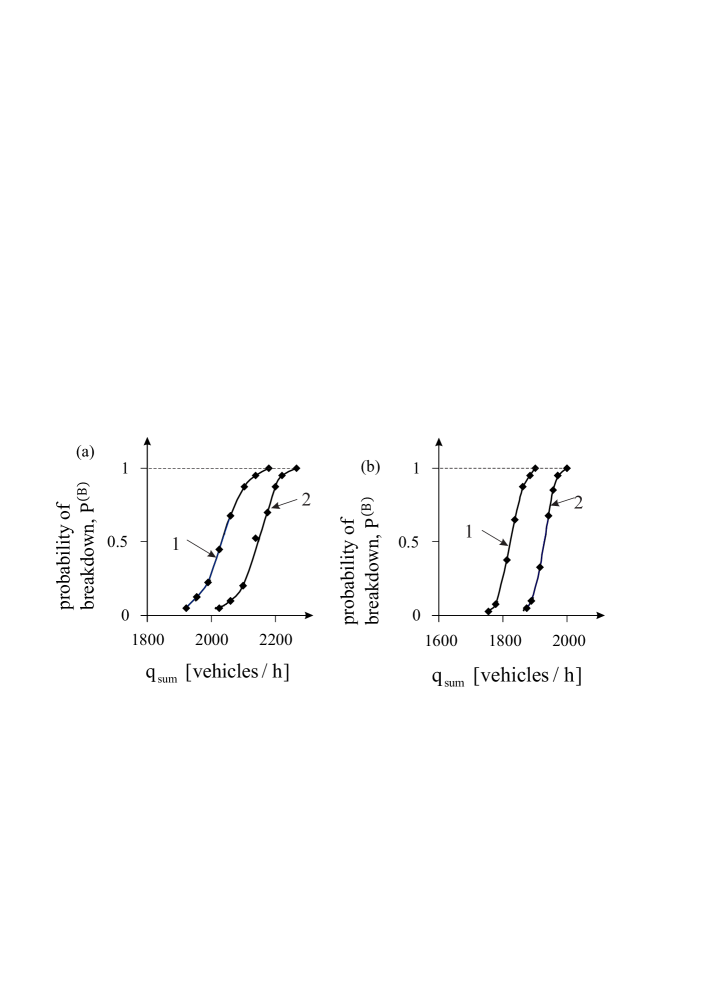
Figure 3: Simulated flow-rate dependencies of probabilities of traffic breakdown at an on-ramp bottleneck on single-lane road [521]: (a) On-ramp inflow rate $q_{\rm on}=$ 60 vehicles/h. (b) On-ramp inflow rate $q_{\rm on}=$ 200 vehicles/h. Curves 1 and 2 in (a, b) are related, respectively, to two different values of time interval for observing traffic flow $T_{\rm ob}=$ 30 (curves 1) and 15 min (curves 2). $q_{\rm sum}=q_{\rm in}+q_{\rm on}$, where $q_{\rm in}$ is the flow rate in free flow on the main road upstream of the bottleneck.

2.2 Threshold flow rate for spontaneous traffic breakdown

For a qualitative analysis of conditions (1), (2), and the flow-rate function of the breakdown probability $P^{\rm(B)}(q_{\rm sum})$ (3) [200, 201, 216, 217, 218, 219, 220, 221, 222], [223, 224, 225, 226, 227, 228, 229, 230], we recall firstly that a nucleus for traffic breakdown (F$\rightarrow$S transition) at a bottleneck is a time-limited local disturbance in free traffic flow that occurrence leads to the breakdown. Clearly that in free flow there can be many time-limited local disturbances with different amplitudes, i.e., many different nuclei that lead to traffic breakdown at the bottleneck. A local disturbance with a minimum amplitude that leads to the breakdown can be called a critical local disturbance. Respectively, the critical local disturbance determines a critical nucleus required for traffic breakdown at the bottleneck.

We can assume that the larger is the flow rate in free flow, the smaller is the critical nucleus required to initiate spontaneous traffic breakdown in metastable free flow at a bottleneck. Obviously, the probability of the occurrence of a small speed disturbance in free flow is considerably larger than the probability of the occurrence of a large disturbance. This means that probability of the spontaneous occurrence of a nucleus for traffic breakdown $P^{\rm(B)}_{\rm nucleus}(q)$ is an increasing function of the flow rate. In accordance with (1), this explains the increasing flow rate function of the breakdown probability $P^{\rm(B)}(q_{\rm sum})$ (3).

As an example of this qualitative discussion of condition (1), we assume that a nucleus for traffic breakdown at a highway bottleneck occurs in free flow that is associated with a time-limited critical local decrease in the speed in an initial free flow at the bottleneck denoted by $\Delta v^{\rm(FS)}_{\rm cr}$ (Fig. 4(a)). The larger the flow rate in free flow, the smaller should be the value $\Delta v^{\rm(FS)}_{\rm cr}$ that initiates the breakdown in free flow. The related decreasing function $\Delta v^{\rm(FS)}_{\rm cr}(q_{\rm sum})$, which is qualitatively shown in Fig. 4(a), has indeed been found in simulations with Kerner-Klenov stochastic microscopic three-phase traffic flow model [520].

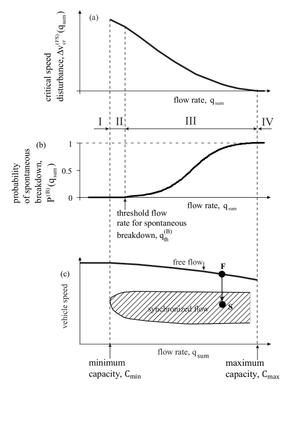
Figure 4: Qualitative explanations of condition (1)  [200, 201, 216, 217, 218, 219, 220, 221, 222], [223, 224, 225, 226, 227, 228, 229, 230]: (a) Qualitative flow rate dependence of function $\Delta v^{\rm(FS)}_{\rm cr}(q_{\rm sum})$. (b) Breakdown probability $P^{\rm(B)}(q_{\rm sum})$ related to formula (3). (c) Z-characteristic for traffic breakdown; arrow in (c) denotes an F$\rightarrow$S transition from a free flow state F to a synchronized flow state S.

At very small flow rates

$$q_{\rm sum}<C_{\rm min},$$ (4)

no traffic breakdown can occur (flow rate range I in Fig. 4). Therefore, there can be no a time-limited speed disturbance in free flow at the bottleneck that can be a nucleus for the breakdown. In flow rate range II, satisfying condition

$$C_{\rm min}\leq q_{\rm sum}<q^{\rm(B)}_{\rm th},$$ (5)

there can be a time-limited speed disturbance in free flow at the bottleneck that can be a nucleus for the breakdown; in (5), $q^{\rm(B)}_{\rm th}$ is a threshold flow rate for spontaneous traffic breakdown (Fig. 4 (a, b)). We assume that under condition (5) a very large value $\Delta v^{\rm(FS)}_{\rm cr}$ (large nucleus) is required for the breakdown, so that the probability of spontaneous occurrence of such very large speed disturbance in free flow during a given time interval $T_{\rm ob}$ is zero, i.e., $P^{\rm(B)}_{\rm nucleus}=0$. In accordance with (1), the probability of spontaneous traffic breakdown

$$P^{\rm(B)}=0.$$ (6)

This means that in this case only induced traffic breakdown is possible. In flow rate range III satisfying condition

$$q^{\rm(B)}_{\rm th}\leq q_{\rm sum}<C_{\rm max},$$ (7)

due to the increase in the flow rate $q_{\rm sum}$ the value $\Delta v^{\rm(FS)}_{\rm cr}(q_{\rm sum})$ required for the breakdown should decrease sharply. For this reason, the probability of the spontaneous occurrence of such a speed disturbance during the time interval $T_{\rm ob}$ can satisfy conditions $0<P^{\rm(B)}_{\rm nucleus}(q_{\rm sum})<1$ and, therefore, in accordance with (1), the probability of spontaneous breakdown

$$0<P^{\rm(B)}(q_{\rm sum})<1.$$ (8)

This consideration explains the sense of the threshold flow rate $q^{\rm(B)}_{\rm th}$: At $q_{\rm sum}=q^{\rm(B)}_{\rm th}$ the breakdown probability is very small but it is still larger than zero. This definition of the threshold flow rate $q^{\rm(B)}_{\rm th}$ for spontaneous traffic breakdown explains why in (5) we assume that at any flow rate $q_{\rm sum}<q^{\rm(B)}_{\rm th}$ the probability of spontaneous traffic breakdown during the time interval $T_{\rm ob}$ is equal to zero (6). In flow rate range IV satisfying condition

$$q_{\rm sum}\geq C_{\rm max},$$ (9)

the value $\Delta v^{\rm(FS)}_{\rm cr}(q_{\rm sum})$ required for the breakdown is as small as zero; therefore, during the time interval $T_{\rm ob}$ the probability of the nucleus occurrence $P^{\rm(B)}_{\rm nucleus}=1$, and, therefore, in accordance with (1), the probability of spontaneous breakdown

$$P^{\rm(B)}(q_{\rm sum})=1.$$ (10)

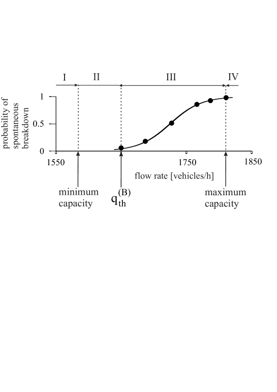
Figure 5: Simulations of flow rate ranges I–IV (4)–(9) for spontaneous and induced traffic breakdowns at on-ramp bottleneck: Typical dependence of the probability of spontaneous traffic breakdown $P^{\rm(B)}(q_{\rm sum})$ on the flow rate $q_{\rm sum}$ calculated with the use of the KKSW CA model for different flow rates $q_{\rm in}$ in free flow upstream of the bottleneck at given $q_{\rm on}=$ 400 vehicles/h. Function $P^{\rm(B)}(q_{\rm sum})$ is related to formula (3). Calculated minimum capacity $C_{\rm min}=$ 1585 vehicles/h. Calculated threshold flow rate $q^{\rm(B)}_{\rm th}\approx 1650$ vehicles/h. Calculated maximum capacity $C_{\rm max}=$ 1810 vehicles/h. $T_{\rm ob}=$ 30 min. Taken from [524].

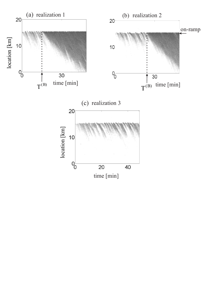
Figure 6: Spontaneous traffic breakdown in KKSW CA model under conditions (7): Speed data presented by regions with variable shades of gray (in white regions the speed is equal to or higher than 120 km/h, in black regions the speed is zero). Three different simulation realizations 1–3 in (a–c) are related to $P^{\rm(B)}=$ 0.775 calculated at $q_{\rm in}=$ 1364 vehicles/h and $q_{\rm on}=$ 400 vehicles/h; different realizations are related to different initial values (at $t=0$) of random model variables. Location of the on-ramp bottleneck is $x_{\rm on}=$ 15 km. Taken from [524].

This qualitative discussion of the basic assumption of the three-phase theory (1) [200, 201, 216, 217, 218, 219, 220, 221, 222], [223, 224, 225, 226, 227, 228, 229, 230] is confirmed by numerical simulations made with the use of the KKSW CA model presented in Figs. 5 and 6 [524]. Simulations show that under condition (4) no traffic breakdown can be either induced or occur spontaneously. Under condition (5), traffic breakdown can be induced at a bottleneck only (Fig. 5). Under condition (7), the breakdown can either be induced or it can occur spontaneously (Figs. 6 (a, b)). There is a time delay for spontaneous traffic breakdown $T^{\rm(B)}$ that is a random value for different simulation realizations (compare values of $T^{\rm(B)}$ for spontaneous traffic breakdown occurring in two different simulation realizations 1 and 2 that are related to the same set of the flow rates $q_{\rm on}$ and $q_{\rm in}$ in Fig. 6 (a, b)). Because under condition (7) we get $0<P^{\rm(B)}(q_{\rm sum})<1$, in some of the simulation realizations no spontaneous breakdown occurs during a chosen observation time for traffic variables $T_{\rm ob}$, as shown for realization 3 in Fig. 6 (c). In this case, traffic breakdown can nevertheless be induced during the observation time $T_{\rm ob}$. Under condition (9), traffic breakdown occurs spontaneously in each of the simulation realizations, i.e., the breakdown probability $P^{\rm(B)}=1$.

2.3 Accuracy of determination of characteristics of probability of traffic breakdown

As in a study of the flow-rate dependence of the empirical breakdown probability $P^{\rm(B)}$ [10, 139], in numerical calculations of the breakdown probability $P^{\rm(B)}(q_{\rm sum})$ [521] only a finite number $N$ of simulation realizations (runs) can be made for the calculation of the value $P^{\rm(B)}$ for each given flow rate $q_{\rm sum}$. In accordance with the definition of the threshold flow rate $q^{\rm(B)}_{\rm th}$, the smallest value of the breakdown probability $P^{\rm(B)}$ that is still larger than zero reaches at the flow rate $q_{\rm sum}=q^{\rm(B)}_{\rm th}$. Thus, the smallest value of the breakdown probability satisfying condition (8) is given by formula

$$P^{\rm(B)}\mid_{q_{\rm sum}=q^{\rm(B)}_{\rm th}}=\frac{1}{N}.$$ (11)

In other words, the larger the number $N$ of simulation realizations (runs), the more exactly the threshold flow rate $q_{\rm sum}=q^{\rm(B)}_{\rm th}$ can be calculated. Correspondingly, an approximate value of $C_{\rm max}$ is found from condition

$$P^{\rm(B)}\mid_{q_{\rm sum}=C_{\rm max}}=\frac{N-1}{N}.$$ (12)

2.4 Dependence of characteristics of breakdown probability on heterogeneity of traffic flow

As shown in real field traffic data [246], empirical spontaneous traffic breakdown is caused by the propagation of a wave in free flow through a permanent speed disturbance localized at a bottleneck. The wave is associated with slow moving vehicles in heterogeneous traffic flow. The slow moving vehicles can be considered $``$moving bottleneck”. Therefore, to explain the basic importance of the function $P^{\rm(B)}(q_{\rm sum})$ for transportation science, we consider simulations of traffic breakdowns in a heterogeneous traffic flow with a moving bottleneck and in traffic flow without moving bottlenecks (Fig. 7).

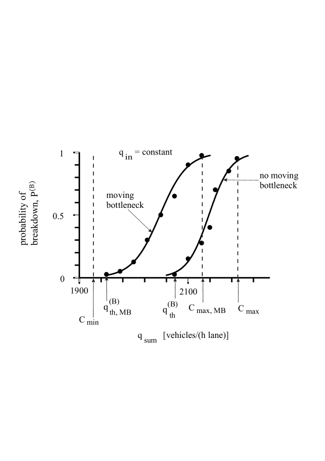
Figure 7: Simulations of probabilities of traffic breakdown in traffic flows with the moving bottleneck and without moving bottlenecks with Kerner-Klenov stochastic three-phase traffic flow model on a two-lane road with on-ramp bottleneck: Probabilities of traffic breakdown $P^{\rm(B)}(q_{\rm sum})$ in traffic flow of identical drivers and vehicles with moving bottleneck (left curve labeled by $``$moving bottleneck”) and without moving bottlenecks (right curve labeled by $``$no moving bottleneck”) as functions of the flow rate downstream of the bottleneck $q_{\rm sum}=q_{\rm in}+0.5q_{\rm on}$ that is varied through the change in the on-ramp inflow rate $q_{\rm on}$ at constant $q_{\rm in}=$ 1800 vehicles/h. Functions $P^{\rm(B)}(q_{\rm sum})$ are described by formula (3). $C_{\rm min}\approx$ 1925 vehicles/(h lane). Taken from [246].

We have found that at any chosen set of the flow rates $(q_{\rm in},\ q_{\rm on})$, the moving bottleneck results in the increase in the probability for traffic breakdown in comparison with the breakdown probability in traffic flow without moving bottlenecks. In other words, the function $P^{\rm(B)}(q_{\rm sum})$ for traffic flow with the moving bottleneck is shifted to the left in the flow rate axis in comparison with the function $P^{\rm(B)}(q_{\rm sum})$ for traffic flow without moving bottlenecks (Fig. 7).

We have also found that the moving bottleneck results in the decrease in both the maximum capacity $C_{\rm max}$ and the threshold flow rate for spontaneous traffic breakdown $q^{\rm(B)}_{\rm th}$. To distinguish the cases of traffic flows with the moving bottleneck and without moving bottlenecks, we denote the maximum capacity $C_{\rm max}$ and the threshold flow rate $q^{\rm(B)}_{\rm th}$ for traffic flow with the moving bottleneck by $C_{\rm max,\ MB}$ and $q^{\rm(B)}_{\rm th,\ MB}$, respectively (Fig. 7).

In contrast with values $C_{\rm max}$ and $q^{\rm(B)}_{\rm th}$, the minimum capacity $C_{\rm min}$ does not depend on whether there is a moving bottleneck in traffic flow or not. This is because at the given flow rate $q_{\rm in}$ the minimum capacity $C_{\rm min}$ shown in Fig. 7 determines the smallest flow rate $q_{\rm on}$ at which traffic breakdown can still be induced at the bottleneck.

2.5 Effect of cooperative vehicles on breakdown probability

Wireless vehicle communication, which is the basic technology for ad-hoc vehicle networks, is one of the most important scientific fields of ITS. This is because there can be many applications of ad-hoc vehicle networks for so-called $``$cooperative driving” in vehicular traffic, including systems for danger warning, adaptive assistance systems, traffic information, improving of traffic flow characteristics, etc. (see, e.g., [605, 606, 607, 608, 609, 610, 611, 612, 613]). As emphasized in Sec. 1.4, the classical traffic flow models used in all known traffic simulation tools cannot explain features of traffic breakdown (F$\rightarrow$S transition) as observed in real measured traffic data. Therefore, these traffic simulation tools cannot be used for the reliable analysis of the effect of an ad-hoc network on traffic flow. For this reason, we review briefly only results of the application of traffic flow models in the framework of the three-phase theory for the analysis of the effect of cooperative vehicles on traffic flow.

Davis was one of the first who applied hypotheses of the three-phase theory for simulations of the cooperative merging at an on-ramp bottleneck to study the prevention of the formation of synchronized flow at the bottleneck [558]. In [539], for a study of cooperative driving we have developed $``$a united network model” that incorporates both a model of ad-hoc network and the Kerner-Klenov three-phase microscopic stochastic traffic flow model.

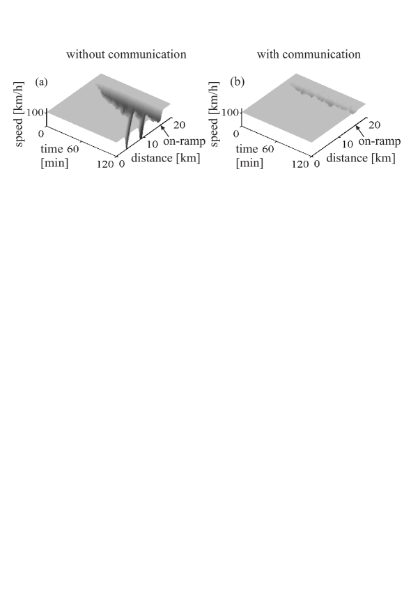
Figure 8: Simulations of prevention of traffic breakdown at on-ramp bottleneck through vehicle communication: Speed in time and space without communication (a) and with vehicle communication (b). Taken from [540].

Figure 9: Simulations of flow-rate functions of probabilities of traffic breakdown $P^{\rm(B)}(q_{\rm sum})$ made with Kerner-Klenov stochastic three-phase model on a two-lane road with on-ramp bottleneck: Traffic flows with V2V-communication (left curve denoted by $``$with communication”) and without V2V-communication (right curve denoted by $``$without communication”). The flow rate downstream of the bottleneck $q_{\rm sum}=q_{\rm in}+0.5q_{\rm on}$ is varied through the change in the on-ramp inflow rate $q_{\rm on}$ at constant $q_{\rm in}=$ 1800 vehicles/h. $C_{\rm min}\approx$ 1925 vehicles/(h lane). Function $P^{\rm(B)}(q_{\rm sum})$ denoted by $``$without communication” is the same as that denoted by $``$no moving bottleneck” in Fig. 7. Functions $P^{\rm(B)}(q_{\rm sum})$ are described by formula (3).

In simulations based on this model [540] (Fig. 8), we assume that vehicles moving in the on-ramp lane send a message for neighbor vehicles moving in the right road lane when the vehicle intends to merge from the on-ramp onto the main road. We assume that the following vehicle in the right lane increases a time headway for the vehicle merging to satisfy a safe gap between the merging vehicle and the following vehicle in the right lane of the main road. Simulations show that in comparison with the case in which no V2V-communication is applied and traffic breakdown occurs (Fig. 8 (a)) this change in driver behavior of communicating vehicles decreases disturbances in free flow at the bottleneck. This results in the prevention of traffic breakdown (Fig. 8 (b)).

The effect of the cooperative merging of vehicles from the on-ramp onto the main road on the breakdown probability is shown in Fig. 9. We can see that the cooperative merging (that is the same as that in Fig. 8 (b)) leads to slight increases in the threshold flow rate for spontaneous traffic breakdown (spontaneous F$\rightarrow$S transition) as well as in the maximum capacity denoted for the case of the cooperative merging by $q^{\rm(B)}_{\rm th,\ com}$ and $C_{\rm max,\ com}$ in comparison with the threshold flow rate $q^{\rm(B)}_{\rm th}$ and the maximum capacity $C_{\rm max}$ related to traffic flow without V2V-communication. The minimum capacity $C_{\rm min}$ is not affected through the cooperative merging. The physics of these results is as follows. The cooperative merging decreases the mean amplitude of speed disturbances occurring through the vehicle merging from the on-ramp onto the main road. For this reason, the cooperative merging increases the threshold flow rate for the spontaneous traffic breakdown and the maximum capacity. The minimum capacity $C_{\rm min}$ determines the threshold for the induced traffic breakdown. The cooperative merging does not affect the possibility of the induced traffic breakdown, therefore, no change in $C_{\rm min}$ has been found.

A study of the effect of moving bottlenecks and cooperative systems on the breakdown probability presented above (Figs. 7 and 9) shows that the characteristics of the breakdown probability $P^{\rm(B)}(q_{\rm sum})$ are the basis characteristics of traffic flow. Therefore, we can make the following conclusions.

• A proof of whether ITS improve traffic flow or not can be made through an analysis of whether there is a shift of the flow-rate function of the breakdown probability $P^{\rm(B)}(q_{\rm sum})$ to the larger flow rates $q_{\rm sum}$ or not. The larger this shift is, the more the effect of ITS on the increase in stochastic highway capacity.

We will use this criterion for an analysis of the effect of automatic driving vehicle on traffic flow in Secs. 4.5 and 5. However, before we consider the nature of empirical stochastic highway capacity.

3 Stochastic highway capacity: Classical theory versus three-phase theory

3.1 Classical understanding of stochastic highway capacity

The classical understanding of highway capacity is defined through the occurrence of traffic breakdown at a bottleneck: The highway capacity is equal to the flow rate in an initially free flow at the bottleneck at which traffic breakdown is observed at the bottleneck [2, 5, 6, 7, 8, 9, 10, 11], [12, 13, 14, 15, 16, 17].

As above-explained, empirical traffic breakdown exhibits the probabilistic nature (Sec. 1.1) [9, 10, 11],  [12, 13, 14, 15, 16, 17]. Respectively, Brilon [12, 13, 14, 15, 16, 17] has introduced the following definition for stochastic highway capacity that is in agreement with the classical capacity definition: Brilon’s stochastic highway capacity $C$ is equal to the flow rate $q_{\rm sum}$ in an initially free flow at the bottleneck at which traffic breakdown is observed at the bottleneck. At any time instant, there is a particular value of stochastic capacity of free flow at the bottleneck. However, as long as free flow is observed at the bottleneck, this particular value of stochastic capacity cannot be measured. Therefore, stochastic capacity is defined through a capacity distribution function $F^{\rm(B)}_{\rm C}(q_{\rm sum})$ [12, 13, 14, 15]:

$$F^{\rm(B)}_{\rm C}(q_{\rm sum})=p(C\leq q_{\rm sum}),$$ (13)

where $p(C\leq q_{\rm sum})$ is the probability that stochastic highway capacity $C$ is equal to or smaller than the flow rate $q_{\rm sum}$ in free flow at a highway bottleneck.

Thus the basic theoretical assumption of the classical understanding of stochastic highway capacity is that traffic breakdown is observed at a time instant $t$ at which the flow rate $q_{\rm sum}$ reaches the capacity $C(t)$. This means that the flow rate function of the probability of traffic breakdown $P^{\rm(B)}(q_{\rm sum})$ should be determined by the capacity distribution function $F^{\rm(B)}_{\rm C}(q_{\rm sum})$ [12, 13, 14, 15]:

$$P^{\rm(B)}(q_{\rm sum})=F^{\rm(B)}_{\rm C}(q_{\rm sum}).$$ (14)

It must be noted that the breakdown probability function found in empirical observations is the empirical evidence. However, condition (14) is a theoretical hypothesis only. This is because in contrast with the breakdown probability function $P^{\rm(B)}(q_{\rm sum})$, the capacity distribution function $F^{\rm(B)}_{\rm C}(q_{\rm sum})$ cannot be measured [12, 13, 14, 15, 16, 17].

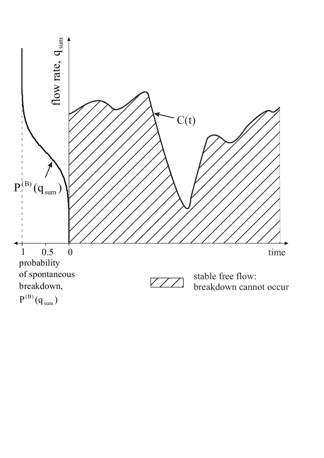
Figure 10: Qualitative explanation of Brilon’s stochastic highway capacity (14) of free flow at a highway bottleneck: Figure left is the flow rate function of the probability of the spontaneous breakdown $P^{\rm(B)}(q_{\rm sum})$. Figure right is a hypothetical fragment of stochastic highway capacity $C(t)$ over time.

This understanding of stochastic capacity of free flow at a bottleneck is qualitatively illustrated in Fig. 10, right, where we show a qualitative hypothetical fragment of the time-dependence of stochastic capacity $C(t)$. Left in Fig. 10, a qualitative flow rate dependence of the probability of spontaneous traffic breakdown $P^{\rm(B)}(q_{\rm sum})$ is shown. The stochastic capacity $C(t)$ can stochastically change over time (Fig. 10). It is often assumed that a stochastic behavior of highway capacity is associated with a stochastic change in traffic parameters over time. Examples of the traffic parameters, which can indeed be stochastic time-functions in real traffic, are weather, mean driver’s characteristics (e.g., mean driver reaction time), share of long vehicles, etc.

Below we will show that the classical understanding of stochastic highway capacity (14), which is generally accepted in transportation research community, contradicts basically the nucleation nature of traffic breakdown in real traffic (Sec. 1.3).

3.2 Characteristics of stochastic highway capacities in three-phase theory

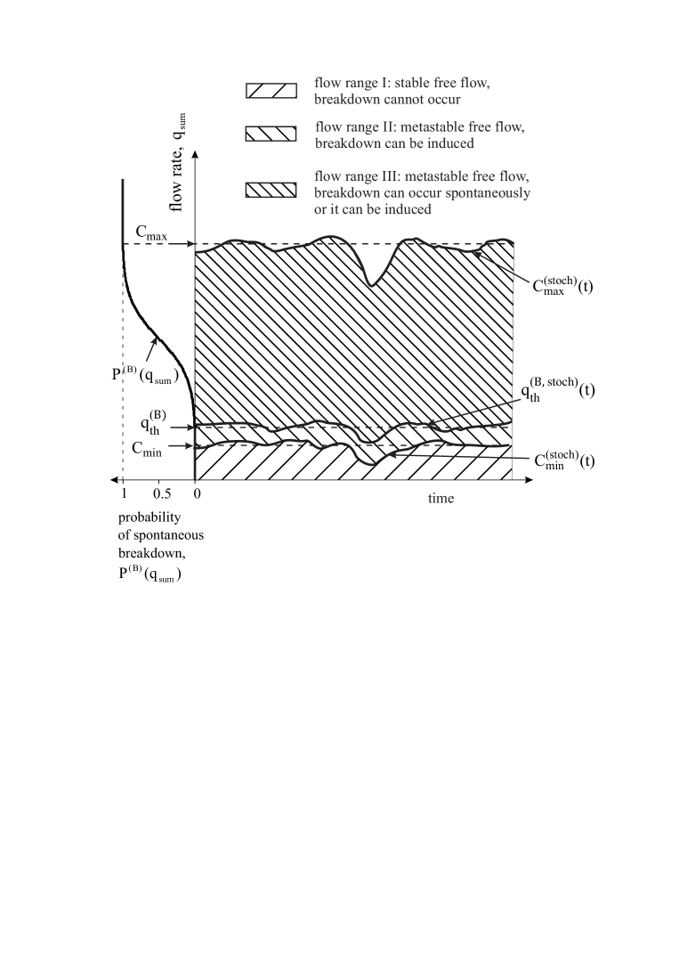
Figure 11: Qualitative explanation of the infinite number of capacities of free flow at a highway bottleneck in three-phase traffic theory. Probability function for traffic breakdown $P^{\rm(B)}(q_{\rm sum})$ (figure left) is the same as that shown in Figs. 10 (left) and 4(b). Flow rate regions I, II, and III mentioned in labeling are, respectively, the same as those shown in Fig. 4 (b) and explained in Sec. 2.2.

It must be noted that the maximum capacity $C_{\rm max}$, the minimum capacity $C_{\rm min}$, and the value $q^{\rm(B)}_{\rm th}$ depend on traffic parameters, like weather, mean driver’s characteristics (e.g., mean driver reaction time), share of long vehicles, etc. In real traffic flow, these traffic parameters change over time. For this reason, the values $C_{\rm max}$, $C_{\rm min}$, and $q^{\rm(B)}_{\rm th}$ change also over time. Moreover, in real traffic flow, the traffic parameters are stochastic time functions. Therefore, in real traffic flow we should consider some stochastic maximum capacity $C^{\rm(stoch)}_{\rm max}(t)$, stochastic minimum capacity $C^{\rm(stoch)}_{\rm min}(t)$, and a stochastic threshold flow rate $q^{\rm(B,\ stoch)}_{\rm th}(t)$ whose time dependence is determined by stochastic characteristics of traffic parameters. Qualitative hypothetical fragment of these time-functions within a time interval is shown in Fig. 11 (right).

Stochastic functions $C^{\rm(stoch)}_{\rm max}(t)$, $C^{\rm(stoch)}_{\rm min}(t)$, and $q^{\rm(B,\ stoch)}_{\rm th}(t)$ shown in Fig. 11 are qualitative hypothetical functions that cannot be measured in empirical observations. Only their mean values (respectively, $C_{\rm max}$, $C_{\rm min}$, and $q^{\rm(B)}_{\rm th}$) can be found in empirical studies of measured traffic data. In particular, the mean values $C_{\rm max}$ and $q^{\rm(B)}_{\rm th}$ can be found from an empirical study of the flow rate function of the breakdown probability $P^{\rm(B)}(q_{\rm sum})$ (Fig. 4 (b)).

It must be noted that in empirical observations the mean value of the minimum capacity $C_{\rm min}$ can be found from a study of a finite number of different days at which induced traffic breakdowns have been observed at a given bottleneck. The value $C_{\rm min}$ is related to these empirical days of observations only. In other words, it can occur that at another day, which is not within the days used for the calculation of $C_{\rm min}$, traffic breakdown at this bottleneck can be induced at a smaller flow rate $q_{\rm sum}$ than the minimum capacity and the minimum flow rate at which traffic breakdown was induced at this bottleneck in all earlier observations. A similar comment is related to the physical meaning of the mean value of $q^{\rm(B)}_{\rm th}$ and $C_{\rm max}$. To explain this, we should note that with a finite number of measurements it is not possible to find some $``$exact value” of the minimum flow rate at which traffic breakdown can occur. In other words, strictly speaking, mean values $C_{\rm max}$, $C_{\rm min}$, and $q^{\rm(B)}_{\rm th}$ are valid only for the days of the observing of traffic breakdown that have been used for the calculations of these mean values.

From Fig. 11 we can see that in the three-phase theory traffic breakdown cannot occur spontaneously at $``$any flow rate”. Indeed, at any time instant at which the flow rate $q_{\rm sum}$ in free flow is smaller than the minimum capacity $C^{\rm(stoch)}_{\rm min}(t)$, no traffic breakdown can occur at the bottleneck. When the flow rate $q_{\rm sum}$ satisfies conditions (5), specifically,

$$C^{\rm(stoch)}_{\rm min}(t)\leq q_{\rm sum}(t)<q^{\rm(B,\ stoch)}_{\rm th}(t),$$ (15)

traffic breakdown can be induced only. Only under conditions

$$q^{\rm(B,\ stoch)}_{\rm th}(t)\leq q_{\rm sum}(t)<C^{\rm(stoch)}_{\rm max}(t)$$ (16)

traffic breakdown can occur spontaneously with some probability $0<P^{\rm(B)}<1$ during a given observation time.

Thus, we can see in Fig. 11 that in accordance with the highway capacity definition made in three-phase theory, under conditions

$$C^{\rm(stoch)}_{\rm min}(t)\leq q_{\rm sum}(t)<C^{\rm(stoch)}_{\rm max}(t)$$ (17)

at any time instant there is the infinite number of highway capacities at which traffic breakdown can occur with some probability or can be induced at the bottleneck.

3.3 Infinite number of stochastic highway capacities in the classical theory and the three-phase theory

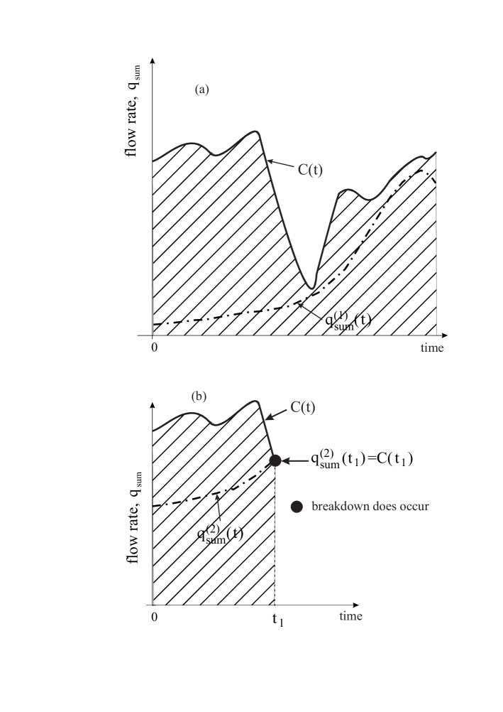
Figure 12: Qualitative explanation of traffic breakdown with the use of Brilon’s stochastic highway capacity of free flow at a highway bottleneck. The fragment of the hypothetical time-function of Brilon’s stochastic highway capacity $C(t)$ is taken from Fig. 10 (right).

In accordance with the classical definition of stochastic capacity (13), (14), no traffic breakdown can occur, when the time dependence of the flow rate is given by a hypothetical time dependence $q^{(1)}_{\rm sum}(t)$ (Fig. 12(a)). This is because the following condition

$$q^{(1)}_{\rm sum}(t)<C(t).$$ (18)

is satisfied at all time instants shown in Fig. 12(a).

In contrast, for another hypothetical time dependence $q^{(2)}_{\rm sum}(t)$ (Fig. 12(b)) traffic breakdown should occur at time instant $t_{1}$ at which

$$q^{(2)}_{\rm sum}(t_{1})=C(t_{1}).$$ (19)

This is because under condition (19) the flow rate $q^{(2)}_{\rm sum}(t)$ is equal to the capacity value (Fig. 12(b)).

In other words, the classical understanding of a particular value of stochastic capacity can be explained as follows: At a given time instant no traffic breakdown can occur at a highway bottleneck if the flow rate $q_{\rm sum}$ in free flow at the bottleneck at the time instant is smaller than the value of the capacity $C$ at this time instant. The basic importance of the words $``$at a given time instant” in the capacity definition is as follows: Because Brilon’s stochastic capacity $C(t)$ changes stochastically over time (Fig. 10), at a given time instant traffic breakdown can occur at the flow rate $q_{\rm sum}$ that is smaller than the value of the stochastic capacity was at another time instant.

In the classical understanding of stochastic capacity, free flow is stable under condition (18). This means that no traffic breakdown can occur or be induced at the bottleneck at long as the flow rate in free flow at the bottleneck is smaller than the stochastic capacity. This contradicts to the empirical fact that traffic breakdown can be induced at the bottleneck due to the upstream propagation of a localized congested pattern (Fig. 2(b)).

This is because stochastic highway capacity cannot depend on whether there is a congested pattern, which has occurred outside of the bottleneck and independent of the bottleneck existence, or not. Indeed, the empirical evidence of induced traffic breakdown is the empirical proof that at a given flow rate at a bottleneck there can be one of two different traffic states at the bottleneck: (i) A state F (free flow) and (ii) a state S (synchronized flow). Due to the upstream propagation of a localized congested pattern, a transition from the state F to the state S, i.e., traffic breakdown is induced. The induced traffic breakdown is impossible to occur under the classical understanding of stochastic highway capacity. This is because in this classical understanding of stochastic highway capacity, free flow is stable under condition (18), i.e., no traffic breakdown can occur (Fig. 12(a)).

In contrast with the classical understanding of stochastic highway capacity, the evidence of the empirical induced breakdown means that free flow is in a metastable state with respect to the breakdown. The metastability of free flow at the bottleneck should exist for all flow rates at which traffic breakdown can be induced at the bottleneck as observed in real traffic (Fig. 2(b)). This empirical evidence of the metastability of free flow at the bottleneck contradicts fundamentally the concept of Brilon’s stochastic capacity, in which free flow is stable under condition (18). This explains why the generally accepted classical understanding of stochastic highway capacity has failed.

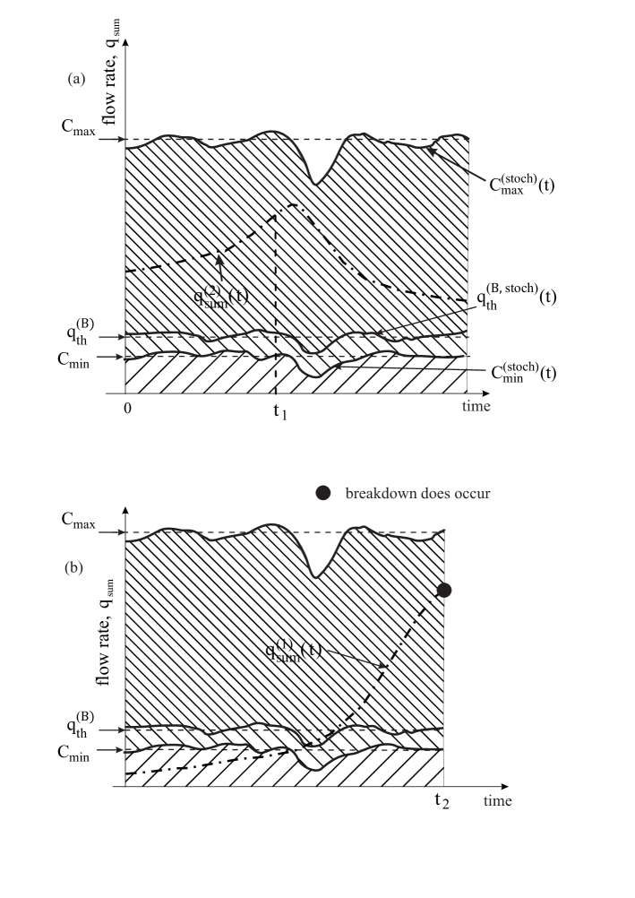
Figure 13: Qualitative explanation of traffic breakdown with the use of the infinite number of capacities of free flow at a highway bottleneck of three-phase theory. Hypothetical time-functions $C^{\rm(stoch)}_{\rm max}(t)$, $C^{\rm(stoch)}_{\rm min}(t)$, and $q^{\rm(B,\ stoch)}_{\rm th}(t)$ are taken from Fig. 11. Hypothetical time functions of the flow rates $q^{(2)}_{\rm sum}(t)$ in (a) and $q^{(1)}_{\rm sum}(t)$ in (b) as well as time instant $t_{1}$ in (a) are, respectively, the same as those in Fig. 12.

The classical understanding of stochastic highway capacity is based on the assumption that the empirical probability of traffic breakdown is determined by the capacity distribution function, i.e., condition (14) is valid. In contrast, the assumption of the three-phase theory about the metastability of traffic breakdown with respect to traffic breakdown (1) is based on the empirical evidence that traffic breakdown can be induced at a bottleneck. In both the classical theory and three-phase theory there is the infinite number of stochastic capacities. However, in the classical understanding of stochastic highway capacity at a given time instant there is only one value of capacity (Fig. 10) that we do not know because the capacity is a stochastic value.

Contrarily, in the three-phase theory at any given time instant there is the infinite number of stochastic capacities within some capacity range between minimum $C^{\rm(stoch)}_{\rm min}$ and maximum capacities $C^{\rm(stoch)}_{\rm max}$. We cannot measure values of $C^{\rm(stoch)}_{\rm max}(t)$ and $C^{\rm(stoch)}_{\rm min}(t)$ because $C^{\rm(stoch)}_{\rm max}(t)$ and $C^{\rm(stoch)}_{\rm min}(t)$ are stochastic values. However, due to the empirical evidence of the possibility of induced traffic breakdown, we know that $C^{\rm(stoch)}_{\rm max}(t)>C^{\rm(stoch)}_{\rm min}(t)$ (Fig. 11). This emphasizes a crucial difference between the sense of the term infinite number of stochastic capacities in the classical theory and the three-phase theory.

Thus the observation of empirical induced breakdowns proves that condition (14) of Brilon’s stochastic capacity cannot be valid for real traffic. However, the following question arises:

• What are the consequences of this controversial understanding of the nature of traffic breakdown?

With the use of Fig. 13, we can qualitatively illustrate the basic difference between the classical understanding of stochastic highway capacity and the understanding of the infinite number of stochastic highway capacities made in the three-phase theory. In the classical understanding of stochastic capacity (14), for the hypothetical time dependence of the flow rate $q^{(2)}_{\rm sum}(t)$ shown in Fig. 12(b), traffic breakdown has occurred at time instant $t_{\rm 1}$ at which condition (19) is satisfied, i.e., when the flow rate is equal to the capacity value. In contrast, in the three-phase theory for the same time dependence of the flow rate $q^{(2)}_{\rm sum}(t)$, for which conditions (7) are satisfied, no breakdown should be necessarily occur both at time instant $t_{\rm 1}$ and for a later time interval (Fig. 13(a)).

In the classical understanding of stochastic capacity (14), for the hypothetical time dependence of the flow rate $q^{(1)}_{\rm sum}(t)$ shown in Fig. 12(a), traffic breakdown could not occur because for all time instants condition (18) is satisfied. In contrast, in the three-phase theory for the same time dependence of the flow rate $q^{(1)}_{\rm sum}(t)$ traffic breakdown can occur spontaneously with some probability as this is shown for time instant $t_{\rm 2}$ in Fig. 13 (b).

Because the classical understanding of stochastic highway capacity (13), (14) contradicts the empirical nucleation nature of real traffic breakdown, the understanding of stochastic highway capacity made in [12, 13, 14, 15, 16, 17] cannot be used for reliable highway design and highway operations.

4 Enhancement of vehicular traffic through automatic driving vehicles

For a probabilistic analysis of the effect of automatic driving vehicles on traffic flow, we consider a simple case of vehicular traffic on a single-lane road with an on-ramp bottleneck. On the single-lane road, no vehicles can pass. For this reason, automatic driving can be achieved through the use of an adaptive cruise control (ACC) in a vehicle: An ACC-vehicle follows a preceding vehicle automatically based on some ACC dynamics rules of motion. Depending on the dynamic behavior of the preceding vehicle, these ACC-rules determine either automatic acceleration or automatic deceleration of the ACC-vehicle or else the maintaining of time-independent speed. The preceding vehicle can be either a human driving vehicle or an automatic driving vehicle through an ACC-system in the vehicle.

4.1 Classical model of ACC

There can be many different ACC dynamics rules of motion behind the preceding vehicle (e.g., [180, 181, 302, 542, 543, 551, 552, 553, 554, 614, 615, 616, 617],

[618, 619, 620, 621, 622, 623, 624, 625, 626, 627],

[628, 629, 630, 631, 632, 633, 634, 635, 636, 637, 638, 639, 640, 641, 642, 643]). We limit the consideration by a classical model of ACC-vehicle. In the classical ACC model, acceleration (deceleration) $a^{\rm(ACC)}(t)$ of the ACC vehicle is determined by current values of the space gap to a preceding vehicle $g(t)$ and the relative speed $\Delta v(t)=v_{\ell}(t)-v(t)$ measured by the ACC vehicle as well as by a desired space gap $g^{\rm(ACC)}=v(t)\tau^{\rm(ACC)}_{\rm d}$, where $v(t)$ is the speed of the ACC-vehicle, $v_{\ell}(t)$ is the speed of the preceding vehicle, and $\tau^{\rm(ACC)}_{\rm d}$ is a desired net time gap (desired time headway) of the ACC-vehicle to the preceding vehicle(e.g., [180, 181, 302, 499, 500, 501, 502, 503, 504, 505, 506],

[507, 508, 509, 510, 513, 542, 543, 551, 552, 553, 554],

[614, 615, 616, 617, 618, 619, 620, 621, 622, 623, 624, 625],

[626, 627, 628, 635, 636, 637, 638, 639, 640, 641, 642, 643]):

$$a^{\rm(ACC)}(t)=K_{1}(g(t)-v(t)\tau^{\rm(ACC)}_{\rm d})+K_{2}(v_{\ell}(t)-v(t)),$$ (20)

where $K_{1}$ and $K_{2}$ are coefficients of ACC adaptation.

Figure 14: Model of the ACC vehicle

All simulations of human driving vehicles presented below are made with Kerner-Klenov microscopic stochastic three-phase traffic flow model [520]. Because in the Kerner-Klenov model discrete time step is used (Appendix A), we use in the classical ACC-model the discrete time $t=n\tau$, where $n=0,1,2,..$; $\tau=$1 s is time step. Therefore, the space gap to a preceding vehicle is equal to $g_{n}=x_{\ell,n}-x_{n}-d$ and the relative speed is given by $\Delta v_{n}=v_{\ell,n}-v_{n}$ (Fig. 14), where $x_{n}$ and $v_{n}$ are coordinate and speed of the ACC-vehicle, $x_{\ell,n}$ and $v_{\ell,n}$ are coordinate and speed of the preceding vehicle, $d$ is the vehicle length that is assumed the same for all automatic driving and human driving vehicles. Respectively, the current net time gap (time headway) between ACC-vehicle and the preceding vehicle calculated by ACC-vehicle is equal to $\tau^{\rm(net)}_{n}=g_{n}/v_{n}$. Correspondingly, the classical model of the dynamics of ACC-vehicle (20) can be rewritten as follows:

$$a^{\rm(ACC)}_{n}=K_{1}(g_{n}-v_{n}\tau^{\rm(ACC)}_{\rm d})+K_{2}(v_{\ell,n}-v_{n}).$$ (21)

Coefficients of ACC adaptation $K_{1}$ and $K_{2}$ describe the dynamic adaptation of the ACC vehicle when either the space gap is different from the desired one $v_{n}\tau^{\rm(ACC)}_{\rm d}$:

$$g_{n}\neq v_{n}\tau^{\rm(ACC)}_{\rm d}$$ (22)

or the vehicle speed is different from the speed of the preceding vehicle:

$$v_{n}\neq v_{\ell,n}.$$ (23)

If in contrast

$$v_{n}=v_{\ell,n}$$ (24)

and the condition

$$g_{n}=v_{n}\tau^{\rm(ACC)}_{\rm d}$$ (25)

is satisfied, from (21) we obtain that

$$a^{\rm(ACC)}_{n}=0,$$ (26)

i.e., the ACC vehicle moves with a time-independent speed.

The physics of the dynamic equation for the ACC vehicle (21) is as follows. It can be seen that the current time headway $\tau^{\rm(net)}_{n}=g_{n}/v_{n}$ in (21) is compared with the desired time headway $\tau^{\rm(ACC)}_{\rm d}$. If $\tau^{\rm(net)}_{n}>\tau^{\rm(ACC)}_{\rm d}$, then the ACC vehicle automatically accelerates to reduce the time headway to the desired value $\tau^{\rm(ACC)}_{\rm d}$. If $\tau^{\rm(net)}_{n}<\tau^{\rm(ACC)}_{\rm d}$, then the ACC vehicle decelerates automatically to increase the time headway. Moreover, the acceleration and deceleration of the ACC vehicle depend on the current difference between the speed of the ACC vehicle and the preceding vehicle. If the preceding vehicle has a higher speed than the ACC vehicle, i.e., when $v_{\ell,n}>v_{n}$, the ACC vehicle accelerates. Otherwise, if $v_{\ell,n}<v_{n}$ the ACC vehicle decelerates.

In simulations of traffic flow discussed below, there are vehicles that have no ACC system (human driving vehicles) and ACC-vehicles (automatic driving vehicles); we call this traffic flow as $``$mixture traffic flow”. In mixture traffic flow, the ACC vehicles are randomly distributed on the road between human driving vehicles. The percentage of automatic driving vehicles denoted by $\gamma$ is the same value in traffic flow upstream of the bottleneck and in the on-ramp inflow onto the main road.

The ACC vehicles move in accordance with Eq. (21) where, in addition, the following formulas are used:

$$v^{\rm(ACC)}_{{\rm c},n}=v_{n}+\tau\max(-b_{\rm ACC},\min(\lfloor a^{\rm(ACC)}_{n}\rfloor,a_{\rm ACC})),$$ (27)

$$v_{n+1}=\max(0,\min({v_{\rm free},v^{\rm(ACC)}_{{\rm c},n},v_{{\rm s},n}})),$$ (28)

where we have taken into account that we use a discrete-in-space version of the Kerner-Klenov model (Appendix A), $\lfloor z\rfloor$ denotes the integer part of $z$. Through the use of formula (27), acceleration and deceleration of the ACC vehicles are limited by some maximum acceleration $a_{\rm ACC}$ and maximum deceleration $b_{\rm ACC}$, respectively. Owing to the formula (28), the speed of the ACC vehicle $v_{n+1}$ at time step $n+1$ is limited by the maximum speed in free flow $v_{\rm free}$ and by the safe speed $v_{{\rm s},n}$ to avoid collisions between vehicles. The maximum speed in free flow $v_{\rm free}$ and the safe speed $v_{{\rm s},n}$ are chosen, respectively, the same as those in the microscopic model of human driving vehicles (Appendix A). It should be noted that the model of ACC-vehicle merging from the on-ramp onto the main road is similar to that for for human driving vehicles (see Sec. A.9 of Appendix A).

An important characteristic of the ACC-vehicles is a stability of a platoon of the ACC-vehicles called string stability. Liang and Peng [626] have found that for a string stability of the ACC vehicles coefficients of ACC adaptation $K_{1}$ and $K_{2}$ in (20) and the desired time headway of the ACC vehicles $\tau^{\rm(ACC)}_{\rm d}$ should satisfy condition [626]

$$K_{2}>\frac{2-K_{1}(\tau^{\rm(ACC)}_{\rm d})^{2}}{2\tau^{\rm(ACC)}_{\rm d}}.$$ (29)

Below to limit the analysis, we consider the effect of the ACC vehicles on traffic flow only for a relatively short desired time headway of the ACC vehicles $\tau^{\rm(ACC)}_{\rm d}=$ 1.1 s. However, we will use different sets of coefficients $K_{1}$ and $K_{2}$ of ACC adaptation.

4.2 String instability versus S$\rightarrow$F instability of three-phase theory

To understand the effect of the ACC vehicles on traffic flow discussed below, firstly we should understand a crucial difference between the dynamic behaviors of the ACC-vehicles (21) and the dynamic behavior of manual driving vehicles in the three-phase theory. As above-mentioned, the platoon of the ACC-vehicles exhibits a string instability, when (29) is not satisfied. For the string instability of traffic flow consisting of 100$\%$ ACC-vehicles, we find a known result that the string instability is a growing wave of local decrease in speed of ACC-vehicles (Fig. 15 (a–c)).

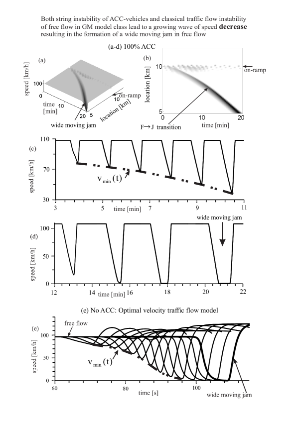
Figure 15: Comparison of string instability in traffic flow of $\gamma=100\%$ of ACC-vehicles at on-ramp bottleneck on single-lane road simulated with classical ACC-model of Sec. 4.1 (a–d) with classical traffic flow instability in traffic flow without ACC-vehicles simulated with OV model [278] belonging to the GM model class (see references in reviews [165, 166, 168, 170, 171, 172, 175, 177, 180, 181, 204]) (e): (a, b) Vehicle speed in space and time (a) and the same speed data presented by regions with variable shades of gray (b) (in white regions the speed is larger than 105 km/h, in black regions the speed is equal to zero). (c–e) Microscopic vehicle speed along vehicle trajectories (only a few of the subsequent trajectories are shown) as time-functions. In (a–d), ACC-parameters are $\tau^{\rm(ACC)}_{\rm d}=1.1$ s, coefficients $(K_{1},\ K_{2})=$ (0.5 $s^{-2}$, 0.2 $s^{-1}$) in (21) do not satisfy condition (29) for string stability; values $a_{\rm ACC}=b_{\rm ACC}=3\ {\rm m}/{\rm s}^{2}$; the flow rates are $q_{\rm on}=50$ vehicles/h, $q_{\rm in}=2609$ vehicles/h ($q_{\rm sum}=q_{\rm on}+q_{\rm in}=2659$ vehicles/h). Figure (e) is taken from [544].

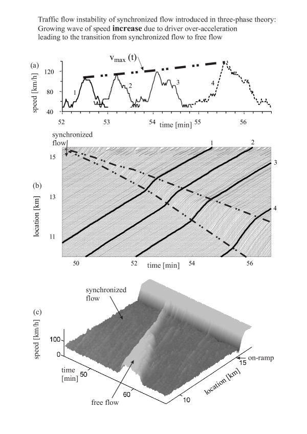
Figure 16: Simulations of S$\rightarrow$F instability introduced in three-phase theory that governs an F$\rightarrow$S transition (traffic breakdown) at on-ramp bottleneck [544]: (a, b) Vehicle speed along trajectories as time-functions (a) and vehicle trajectories in space and time (b); numbers of trajectories in (b) are related to trajectories labeled in (a) by the same numbers. (c) Speed in space and time.

Qualitatively the same growing wave of local decrease in speed occurs due to the classical instability in a platoon of manual driving vehicles moving at free flow speed in accordance with rules of a traffic flow model of the GM model class. As in traffic flow models of the GM model class, this growing wave caused by the string instability of the ACC-vehicles leads to the emergence of a wide moving jam in traffic flow of the ACC-vehicles, i.e., to an F$\rightarrow$J transition (compare Fig. 15 (a–d) for string instability of the ACC-vehicles with well-known results shown in Fig. 15 (e) for the classical traffic flow instability of the GM model class). Thus we can make the conclusions:

• As the classical traffic flow instability of the GM model class (Fig. 15 (e)), string instability of the ACC-vehicles (Fig. 15 (a–c)) is a growing wave of speed reduction in free flow.

• As the classical traffic flow instability (Fig. 15 (e)), the string instability of the ACC-vehicles leads to the formation of wide moving jams in free flow (F$\rightarrow$J transition) (Fig. 15 (a, b, d)).

In contrast with the ACC-vehicles and with the classical traffic flow instability of the GM model class, as explained and proven in a recent paper [544], in the three-phase theory there is no string instability in a platoon of manual driving vehicles moving at free flow speed. Rather than string instability, traffic breakdown in traffic flow that consists only of manual driving vehicles is associated with the existence of an S$\rightarrow$F instability introduced in the three-phase theory. As proven [544], the S$\rightarrow$F instability governs the metastability of free flow with respect to an F$\rightarrow$S transition (traffic breakdown) at a bottleneck as observed in all real field traffic data. As explained in details in [544], the S$\rightarrow$F instability is a growing wave of local increase in speed in synchronized flow (Fig. 16 (a, b)) that leads to the S$\rightarrow$F transition (Fig. 16 (c)). Thus we can make the conclusions:

• Contrary to classical instability of the GM model class and string instability of the ACC-vehicles that lead to speed reduction in free flow (Fig. 15), the S$\rightarrow$F instability of the three-phase theory is a growing wave of local increase in speed in synchronized flow (Fig. 16) [544].

• Contrary to classical instability of the GM model class and string instability of the ACC-vehicles leading to the F$\rightarrow$J transition (Fig. 15 (a, b, d, e)), the S$\rightarrow$F instability of the three-phase theory governs traffic breakdow (F$\rightarrow$S transition)n in free flow [544].

• In the three-phase theory, no string instability occurs in a platoon of manual driving vehicles moving at a free flow speed.

However, it should be noted that the critical conclusion that the classical traffic instability of the GM model class (see references in reviews

[165, 166, 168, 170, 171, 172],

[175, 177, 180, 181, 204]) failed to explain traffic breakdown in real field traffic data (see Sec. 1.4) is not related to the string instability of the platoon of the ACC-vehicles.

The reason for this is as follows: In general, the dynamics rules of motion of an ACC vehicle are related to a fixed program written by ACC-developers, not to some behavior of manual drivers in real traffic flow. Therefore, if the classical rules (21) exhibit a string instability of the platoon of the ACC-vehicles, then this is a feature of the rules (21). This feature of the ACC-vehicle should not necessarily be in agreement with real dynamic rules of motion of manual driving vehicles.

This is crucially different for a traffic flow model that should describe dynamics rules of motion of real manual driving vehicles. In other words, in contrast with the rules of motion of the ACC-vehicles, dynamics rules of motion of manual driving vehicles in the traffic flow model should be in agreement with real field traffic data. The real data reflects the behavior of real manual driving vehicles: The real behavior of drivers results in the empirical evidence that traffic breakdown is the F$\rightarrow$S transition in metastable free flow, not the F$\rightarrow$J transition resulting from simulations of traffic flow models of the GM model class.

This explains why the failure of traffic flow models of the GM model class should not necessarily be considered as a drawback of the classical rules (21) of the dynamics of the ACC-vehicles. Nevertheless, from the analysis of the effect of the classical ACC-vehicles of traffic flow, which will be made below in Sec. 5, we could have an assumption that to improve traffic flow through automatic driving vehicles considerably, the dynamic behavior of the future ACC-vehicles should learn from some behaviors of manual driving vehicles in real traffic flow (see an example in Sec. 6).

4.3 Main objective of analysis of effect of ACC-vehicles on traffic flow

It should be noted that even when condition for string stability (29) is satisfied, nevertheless, traffic congestion occurs in traffic flow consisting of 100$\%$ ACC-vehicles, if the flow rate $q_{\rm sum}$ exceeds the value

$$q_{0}=\frac{3600}{\tau^{\rm(ACC)}_{\rm d}+d/v_{\rm free}}.$$ (30)

For this reason, in all simulations of the effect of ACC-vehicles on traffic flow presented in this mini-review below, we have chosen model parameters at which traffic breakdown occurs in a mixture traffic flow, only when the flow rate at the bottleneck $q_{\rm sum}$ is considerably smaller than $q_{0}$ (30):

$$q_{\rm sum}=q_{\rm on}+q_{\rm in}<q_{0}\approx 2667\ {\rm[vehicles/h]},$$ (31)

where in formula (30) we have taken into account that we consider only ACC-vehicles with $\tau^{\rm(ACC)}_{\rm d}=1.1$ s, $v_{\rm free}=$ 30 m/s, and $d=$ 7.5 m. Under condition (31), it is often expected that if there is string stability of a platoon of the ACC-vehicles, then the ACC-vehicles should improve traffic flow.

• The main objective of our analysis of the effect of the ACC-vehicles on traffic flow presented below is to prove that this assumption should not necessarily be valid, even when condition of string stability for the ACC-vehicles (29) and condition (31) are satisfied.

• We will find that depending on the coefficients of ACC adaptation $K_{1}$ and $K_{2}$ in (21) (which all satisfy condition (29) for string stability) the ACC-vehicles can either improve or deteriorate the traffic system.

Before we consider cases in which the ACC-vehicles under conditions (29) and (31) deteriorate the traffic system (Sec. 5), in Secs. 4.4 and 4.5 we consider expected cases in which the ACC-vehicles enhance the traffic system, specifically, prevent traffic breakdown (Sec. 4.4) or decrease the breakdown probability (Sec. 4.5) .

4.4 Suppression of traffic breakdown through automatic driving vehicles

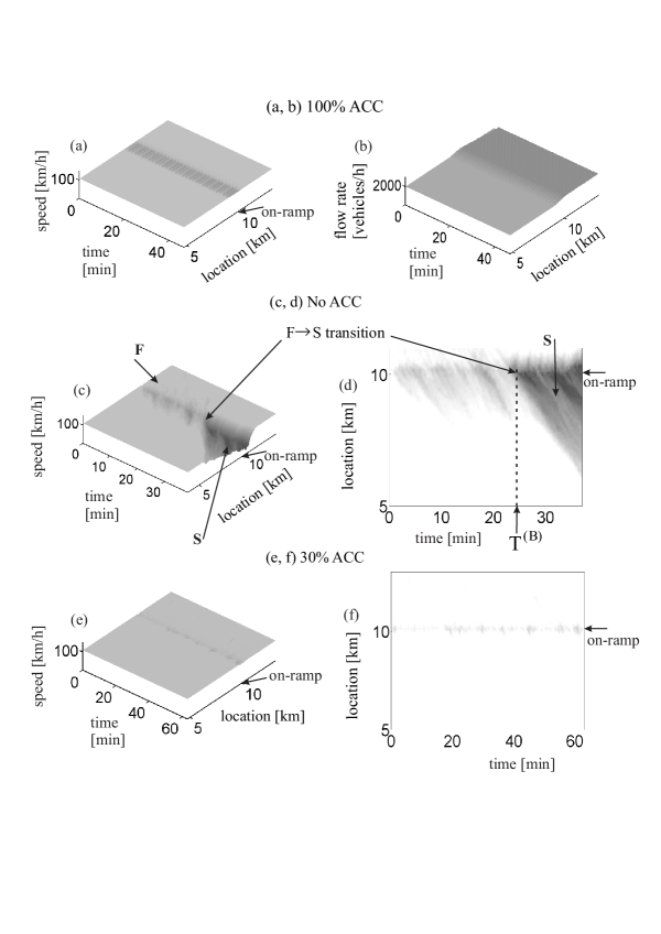
Figure 17: Suppression of F$\rightarrow$S transition in traffic flow on single-lane road with an on-ramp bottleneck through ACC-vehicles: (a, b) Vehicle speed (a) and the flow rate (averaging over 20 vehicles) (b) in space and time. (c–f) Vehicle speed in space and time (c, e) and the same speed data presented by regions with variable shades of gray (d, f) (in white regions the speed is equal to 105 km/h, in black regions the speed is equal to zero). In (a, b), traffic flow with $\gamma=100\%$ of ACC vehicles with $\tau^{\rm(ACC)}_{\rm d}=1.1$ s and coefficients $(K_{1},\ K_{2})=$(0.14 $s^{-2}$, 0.9 $s^{-1}$) satisfying (29); values $a_{\rm ACC}=b_{\rm ACC}=3\ {\rm m}/{\rm s}^{2}$. In (c, d), no ACC vehicles – traffic flow consisting only of human driving vehicles. In (e, f) $\gamma=30\%$ of ACC vehicles with the same parameters as those (a, b). Flow rates in all figures are $q_{\rm on}=320$ vehicles/h, $q_{\rm in}=2000$ vehicles/h ($q_{\rm sum}=q_{\rm on}+q_{\rm in}=2320$ vehicles/h that satisfies (31)). F – free flow, S – synchronized flow. On-ramp location $x_{\rm on}=$ 10 km.

As expected, free flow consisting of $\gamma=100\%$ of ACC vehicles that satisfy conditions (29) and (31) is stable: All speed disturbances occurring due to the merging of ACC-vehicles at the bottleneck decay over time (Fig. 17 (a, b)). However, the disturbances cause a decrease in free flow speed at the bottleneck location seen in Fig. 17 (a): Automatic driving vehicles moving initially on the main road with the speed $v_{\rm free}$ upstream of the bottleneck should decelerate in a neighborhood of the bottleneck due to the merging of other automatic driving vehicles from the on-ramp onto the main road.

At the same flow rates $q_{\rm on}$ to the on-ramp and on the main road $q_{\rm in}$ as those in Fig. 17 (a, b), in free flow consisting only of human driving vehicles (no ACC-vehicles) traffic breakdown occurs at the bottleneck during the time interval $T_{\rm ob}=$ 30 min with the probability $P^{\rm(B)}=$ 0.375 (Fig. 17 (c, d)). In a simulation realization shown in Fig. 17 (c, d), traffic breakdown has occurred after a random time delay $T^{\rm(B)}\approx$ 25 min.

When we consider a mixture traffic flow and increase the percentage $\gamma$ of ACC vehicles in the mixture traffic flow to $\gamma=30\%$, we get a known result derived with different traffic flow models in the framework of the three-phase theory that no traffic breakdown (F$\rightarrow$S transition) occurs (Fig. 17 (e, f)). The work by Davis [551] was one of the first to obtain this result with another human driver model that had some of the features of the three-phase theory.

4.5 Decrease in probability of traffic breakdown through automatic driving vehicles

At a smaller percentage of ACC-vehicles than $\gamma=30\%$ in the mixture traffic flow with the same parameters of the ACC-vehicles and the flow rates as those in Fig. 17, we have found the following results (Fig. 18). As long as the percentage of ACC-vehicles is appreciably smaller than $\gamma=10\%$, no considerable change in the probabilistic features of traffic breakdown at the bottleneck is observed. Even when the percentage of ACC-vehicles increases to $\gamma=10\%$, features of traffic breakdown remains almost the same as those in traffic flow of manual driving vehicles (Fig. 18 (a, b)) and only a relatively small decrease in the probability of the breakdown is observed (Fig. 19 (a), curve labeled by $``$10$\%$ ACC”).

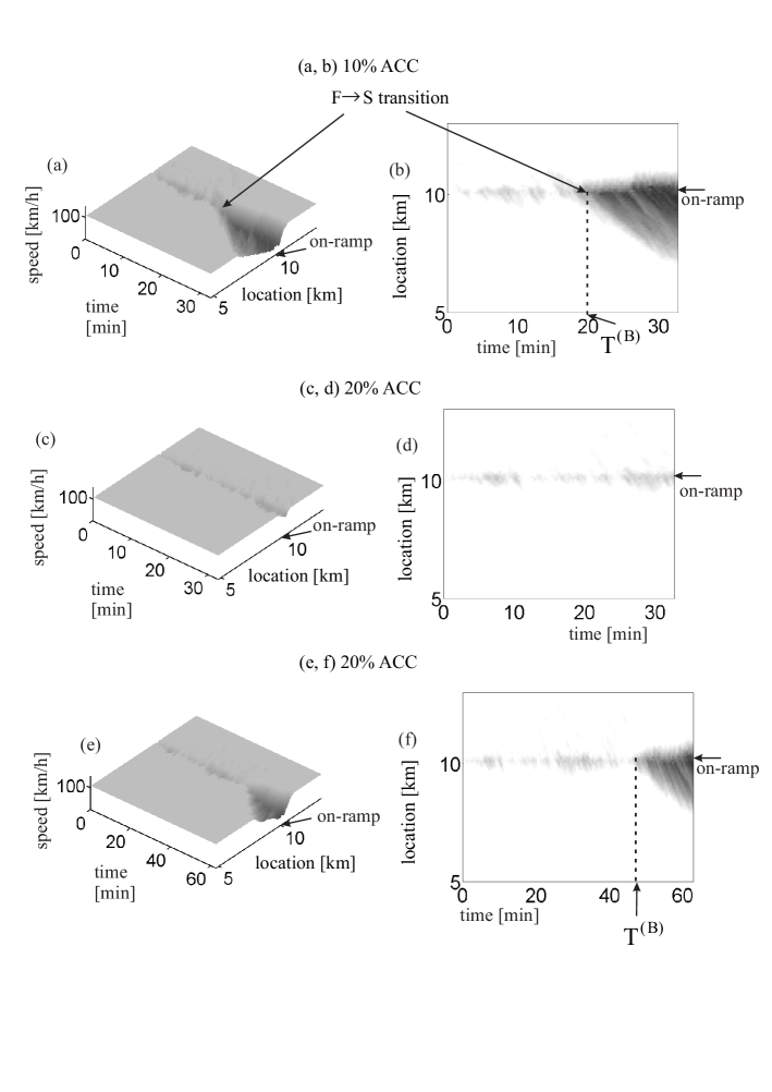
Figure 18: Simulations of the effect of ACC-vehicles on probabilistic characteristic of traffic breakdown: Vehicle speed in space and time (a, c, e) and the same speed data presented by regions with variable shades of gray (b, d, f) (in white regions the speed is equal to 105 km/h, in black regions the speed is equal to zero). (a, b) $\gamma=10\%$. (c–f) $\gamma=20\%$. ACC-parameters are the same as those in Fig. 17. Arrows F$\rightarrow$S in (a, b) mark the F$\rightarrow$S transition (traffic breakdown) at the location of on-ramp bottleneck. F – free flow, S – synchronized flow.

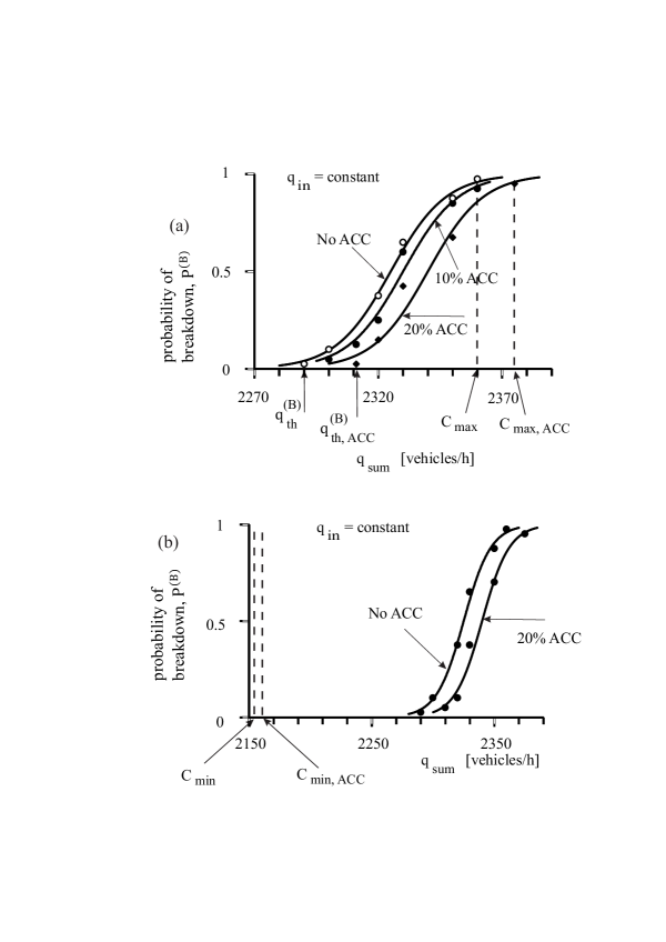
Figure 19: Flow-rate functions of probabilities of traffic breakdown $P^{\rm(B)}(q_{\rm sum})$ in traffic flows without ACC-vehicles (left curves in (a, b) labeled by $``$No ACC”) as well as with 10$\%$ and 20$\%$ of ACC-vehicles (right curves labeled by $``$10$\%$ ACC” and $``$20$\%$ ACC”) as functions of the flow rate downstream of the bottleneck $q_{\rm sum}$; curves $``$No ACC” and $``$20$\%$ ACC” are shown in different flow-rate scales in (a) and (b). The flow rate $q_{\rm sum}=q_{\rm in}+q_{\rm on}$ is varied through the change in the on-ramp inflow rate $q_{\rm on}$ at constant $q_{\rm in}=$ 2000 vehicles/h. To distinguish the cases of traffic flows with the ACC-vehicles and without ACC-vehicles, we denote the maximum capacity $C_{\rm max}$, the minimum capacity $C_{\rm min}$, and the threshold flow rate $q^{\rm(B)}_{\rm th}$ for traffic flow with 20$\%$ of ACC-vehicles by $C_{\rm max,\ ACC}$, $C_{\rm min,\ ACC}$, and $q^{\rm(B)}_{\rm th,\ ACC}$, respectively. Functions $P^{\rm(B)}(q_{\rm sum})$ are described by formula (3). Other model parameters are the same as those in Fig. 17.

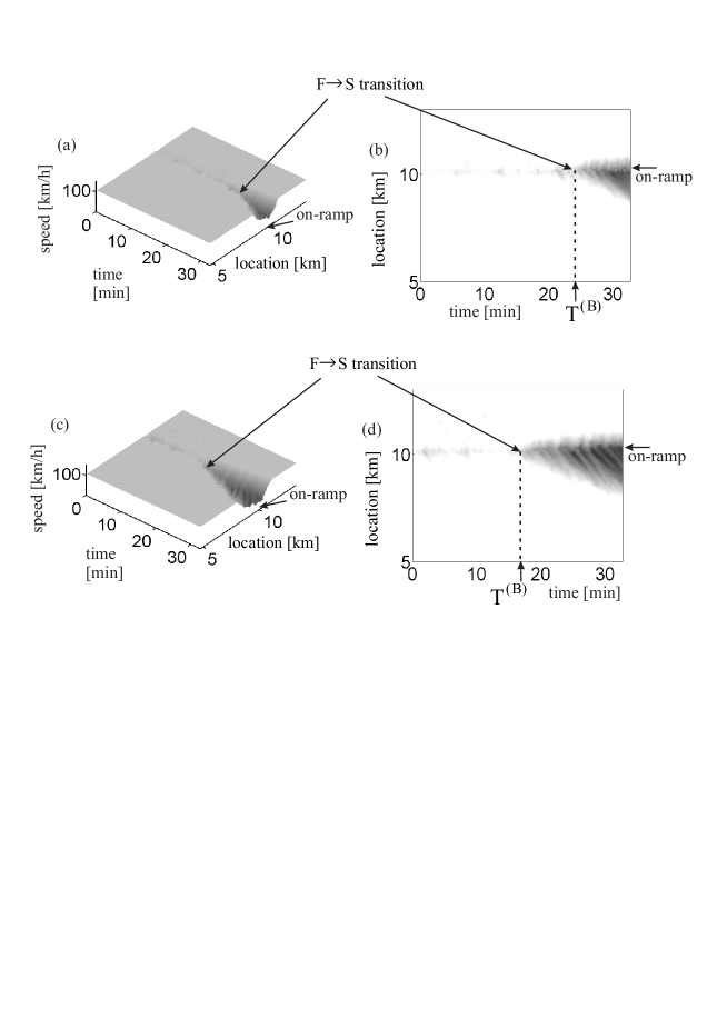
Figure 20: Two different simulation realizations 2 (a, b) and 3 (c, d) of the effect of ACC on probabilistic features of traffic breakdown for $\gamma=20\%$ of ACC vehicles with the same time of observation of traffic flow $T_{\rm ob}=$ 30 min as that in simulation realization 1 in which no breakdown occurs during $T_{\rm ob}=$ 30 min (Fig. 18 (c, d)): Vehicle speed in space and time (a, c) and the same speed data presented by regions with variable shades of gray (b, d) (in white regions the speed is equal to 105 km/h, in black regions the speed is equal to zero). Other model parameters are the same as those in Fig. 17.

Now, in comparison with Fig. 18 (a, b), we increase the percentage $\gamma$ of automatic driving vehicles to $\gamma=20\%$ without any other changes in simulations. We have found that at $\gamma=20\%$ automatic driving vehicles no traffic breakdown occurs during the observation time $T_{\rm ob}=30$ min (Fig. 18 (c, d)). However, if we continue simulations shown Fig. 18 (c, d) during a longer time interval, we have found that after a long time delay $T^{\rm(B)}\approx 47$ min traffic breakdown has nevertheless occurred at the bottleneck (Fig. 18 (c, d)). We have found that the mean time delay of traffic breakdown for $\gamma=20\%$ of ACC vehicles is considerably longer than for traffic flow consisting of only human driving vehicles.

For $\gamma=20\%$ of automatic driving vehicles the probability that traffic breakdown in the mixture traffic flow occurs during the observation time $T_{\rm ob}=30$ min is equal to $P^{\rm(B)}=$ 0.1 for model parameters used in Fig. 18 (c, d). Thus we can expect that in comparison with the simulation realization shown in Fig. 18 (c, d), in which no breakdown is observed, there should be other simulation realizations made at the same parameters of the mixture traffic flow, in which traffic breakdown is observed during the time interval $T_{\rm ob}=30$ min. Such simulation realizations with different random values of time delays $T^{\rm(B)}$ to the breakdown indeed exist (Fig. 20).

The physics of these results can be explained as follows. In traffic flow consisting of human driving vehicles only, traffic breakdown (F$\rightarrow$S transition) occurs (Fig. 17 (c, d)), when a large enough speed disturbance (nucleus for the breakdown) occurs in metastable free flow in a neighborhood of the bottleneck. Free flow that consists of $100\%$ automatic driving vehicles is stable (Fig. 17 (a, b)). For this reason, we can assume that a long enough platoon of ACC-vehicles that propagates through the disturbance can cause the dissolution of the disturbance. The larger the percentage $\gamma$ of automatic driving vehicles in the mixture traffic flow, the larger the probability of the appearance of the long platoon of ACC-vehicles, and, therefore, the larger the probability of the disturbance dissolution and the smaller the breakdown probability $P^{\rm(B)}$.

These qualitative explanations are confirmed by numerical simulations of the flow-rate dependence of the probability of traffic breakdown $P^{\rm(B)}(q_{\rm sum})$ presented in Fig. 19. Indeed, we have found that the flow-rate dependence of the probability of traffic breakdown for the mixture traffic flow with 20$\%$ automatic driving vehicles (right curve $P^{\rm(B)}(q_{\rm sum})$ labeled by $``$20$\%$ ACC” in Fig. 19 (a)) is shifted to larger flow rates in comparison with the function $P^{\rm(B)}(q_{\rm sum})$ for traffic flow consisting of human driving vehicles only (left curve labeled by $``$No ACC” in Fig. 19 (a)).

Correspondingly, we have found that the maximum capacity $C_{\rm max}$ and the threshold flow rate $q^{\rm(B)}_{\rm th}$ for spontaneous traffic breakdown increase for the mixture flow. Traffic flow consisting of human driving vehicles only and mixture traffic flow are different traffic flows. We can expect that the minimum capacities $C_{\rm min}$ can also be different values in these two different traffic flows. Indeed, we have found that in the mixture traffic flow the minimum capacity $C_{\rm min,\ ACC}$ is slightly larger in comparison with the minimum capacity $C_{\rm min}$ in traffic flow consisting of human driving vehicles only (Fig. 19 (b)).

• Automatic driving vehicles can indeed decrease the probability of traffic breakdown in the mixture free flow.

• Automatic driving vehicles can increase the threshold flow rate for spontaneous traffic breakdown as well as the maximum and minimum capacities of free flow at the bottleneck.

5 Deterioration of performance of traffic system through automatic driving vehicles

Rather than the enhancement of traffic flow characteristics (Secs. 4.4 and 4.5), automatic driving vehicles can also result in the deterioration of performance of traffic system. To show this, we consider a mixture traffic flow under condition (31). In this mixture traffic flow, ACC-vehicles exhibit the same short desired time headway $\tau^{\rm(ACC)}_{\rm d}=1.1$ s as used above in Secs. 4.4 and 4.5. Moreover, all sets of dynamics coefficients $K_{1}$ and $K_{2}$ of ACC-vehicles used below (see Fig. 21–23) satisfy condition of string stability (29). Nevertheless, we will find that the ACC-vehicles can lead to a considerable increase in the probability of traffic breakdown at road bottlenecks (Fig. 21).

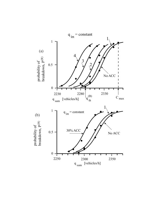
Figure 21: Increase in the probability of traffic breakdown $P^{\rm(B)}$ in mixture free traffic flow through ACC-vehicles with $\tau^{\rm(ACC)}_{\rm d}=1.1$ s: In (a, b), the flow-rate dependence of the breakdown probability $P^{\rm(B)}(q_{\rm sum})$ labeled by $``$No ACC” is taken from Fig. 19 for free flow of manual driving vehicles without ACC-vehicles. In (a), curves $P^{\rm(B)}(q_{\rm sum})$ labeled by numbers 1–4 are related to mixture free flows with $\gamma=5\%$ of ACC-vehicles with different sets of coefficients $(K_{1},\ K_{2})=$ (0.2 $s^{-2}$, 0.82 $s^{-1}$) for curve 1, (0.3 $s^{-2}$, 0.77 $s^{-1}$) for curve 2, (0.5 $s^{-2}$, 0.65 $s^{-1}$) for curve 3, (0.7 $s^{-2}$, 0.55 $s^{-1}$) for curve 4, which satisfy (29); values $a_{\rm ACC}=b_{\rm ACC}=3\ {\rm m}/{\rm s}^{2}$. In (b), curve $P^{\rm(B)}(q_{\rm sum})$ labeled by $``$30$\%$ ACC” is related to mixture free flow with $\gamma=30\%$ of ACC-vehicles with $(K_{1},\ K_{2})=$ (0.2 $s^{-2}$, 0.82 $s^{-1}$); curve 1 is the same as that in (a). The flow rate $q_{\rm sum}=q_{\rm in}+q_{\rm on}$ is varied through the change in the on-ramp inflow rate $q_{\rm on}$ at constant $q_{\rm in}=$ 2000 vehicles/h. Functions $P^{\rm(B)}(q_{\rm sum})$ are described by formula (3).

Indeed, we have found that even a relatively small percentage $\gamma=5\%$ of the ACC-vehicles in the mixture traffic flow can increase considerably the probability of traffic breakdown (Fig. 21 (a), curves 1–4). The importance of this result is as follows: In Secs. 4.4 and 4.5, we have mentioned that the positive effect of the ACC-vehicles on traffic flow, in particular, the decrease in the probability of traffic breakdown is considerable only at large percentages of ACC-vehicles $\gamma\approx 20\%$. In the next future, we could expect only much smaller percentages of automatic driving vehicles in the mixture traffic flow, like $\gamma\approx 5\%$. Therefore, the deterioration of the performance of a mixture traffic flow shown Fig. 21 (a) (curves 1–4) can be a subject of the development of automatic driving vehicles in car-development companies already during next years.

To understand the deterioration of the performance of the traffic system through automatic driving vehicles (Fig. 21), firstly we should note that for each set of dynamic coefficients $(K_{1},\ K_{2})$ of the ACC-vehicles used in simulations shown Fig. 21 (a) (curves 1–4), free flow consisting of $\gamma=100\%$ of the ACC-vehicles is stable: We have found the same results for free flow stability as those presented in Fig. 17 (a, b). This means that when in the mixture free flow the percentage of the ACC-vehicles increases, then, at least under condition $\gamma\rightarrow 100\%$, no traffic breakdown should be observed any more. This has indeed been found in simulations.

We have found that for any of the sets of dynamic coefficients $(K_{1},\ K_{2})$ used in Fig. 21, when the percentage of the ACC-vehicles increases from $\gamma=5\%$ to larger values, firstly, the flow rate dependence of the breakdown probability $P^{\rm(B)}(q_{\rm sum})$ is subsequently shifted to the left in the flow rate axis as shown in Fig. 21 (b) (curve labeled by $``$30$\%$ ACC”).

However, there should be a critical percentage of the ACC-vehicles denoted by $\gamma^{\rm(increase)}_{\rm cr}$. When $\gamma=\gamma^{\rm(increase)}_{\rm cr}$, then the shift of the function $P^{\rm(B)}(q_{\rm sum})$ to the left in the flow rate axis should reach its maximum. When the percentage of ACC-vehicles increases subsequently, i.e, $\gamma>\gamma^{\rm(increase)}_{\rm cr}$, then the function $P^{\rm(B)}(q_{\rm sum})$ should begin to be shifted to the right in the flow rate axis in comparison with the case $\gamma=\gamma^{\rm(increase)}_{\rm cr}$. Finally, as above-mentioned, at $\gamma\rightarrow 100\%$, free flow should occur as long as condition (31) is satisfied.

The above assumption about the behavior of the function $P^{\rm(B)}(q_{\rm sum})$ under increase in the percentage of the ACC-vehicles is indeed confirmed by simulation results, which have been made for each of the sets of dynamic coefficients $(K_{1},\ K_{2})$ of the ACC-vehicles used in Fig. 21. Moreover, it turns out that already for dynamic coefficients $(K_{1},\ K_{2})=$ (0.2 $s^{-2}$, 0.82 $s^{-1}$), which do not considerably differ from $(K_{1},\ K_{2})=$ (0.14 $s^{-2}$, 0.9 $s^{-1}$) used in Figs. 17–19, we have found that $\gamma^{\rm(increase)}_{\rm cr}\approx 30\%$ (curve $P^{\rm(B)}(q_{\rm sum})$ labeled by $``$30$\%$ ACC” in Fig. 21 (b)). This leads to the following result:

• The deterioration of the performance of the traffic system through automatic driving vehicles can occur within broad ranges of the percentage of ACC-vehicles and the set of coefficients $(K_{1},\ K_{2})$, which satisfy condition (29) of string stability of ACC-vehicles.

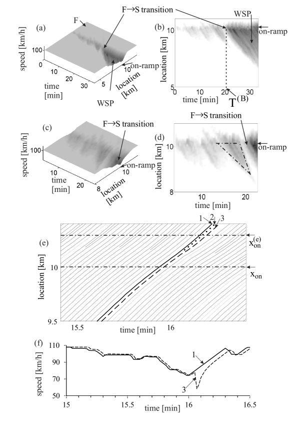
Figure 22: Simulations of dynamics of permanent speed disturbance at on-ramp bottleneck on single-lane road for a mixed traffic flow with $\gamma=5\%$ of ACC-vehicles with coefficients $(K_{1},\ K_{2})=$ (0.5 $s^{-2}$, 0.65 $s^{-1}$): (a–d) Speed in space and time (a, c) and the same data presented by regions with variable shades of gray (b, d) (in white regions the speed is equal to or higher than 105 km/h, in black regions the speed is equal to 0 km/h (b) and smaller than 20 km/h (d)); in (c, d), we show the same data as those in (a, b), however, for smaller space and time intervals. (e) Fragment of vehicle trajectories in space and time related to (c, d). (f) Microscopic vehicle speeds along trajectories as time functions labeled by the same numbers as those in (e). In (d), dashed-dotted lines denote F$\rightarrow$S$\rightarrow$F transitions. F – free flow, WSP – widening synchronized flow pattern. $q_{\rm on}=$ 320 vehicles/h, $q_{\rm in}=$ 2000 vehicles/h.

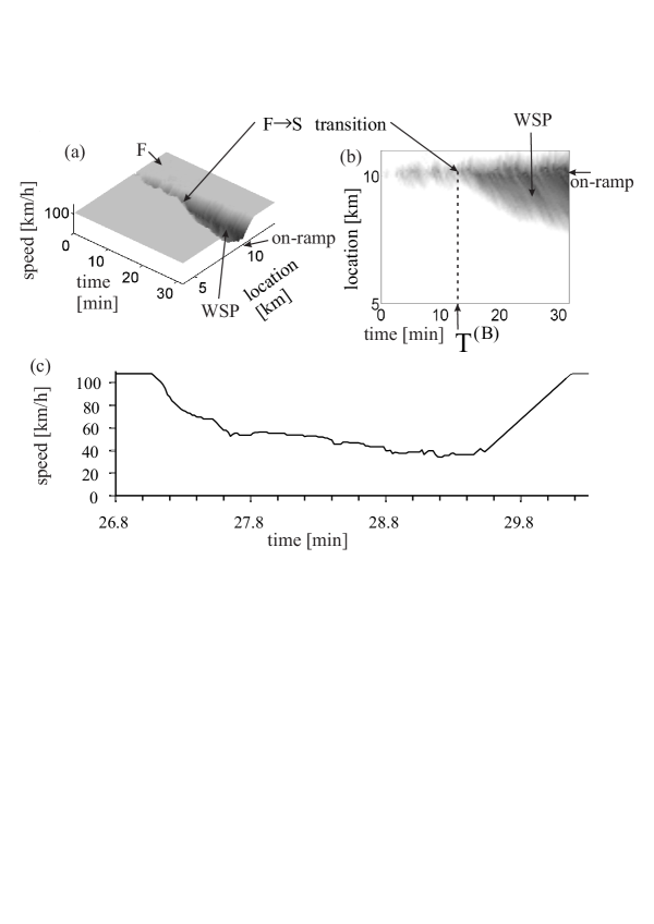
Figure 23: Simulations of F$\rightarrow$S transition (traffic breakdown) at on-ramp bottleneck on single-lane road for mixture traffic flow with $\gamma=30\%$ of ACC-vehicles with $(K_{1},\ K_{2})=$ (0.2 $s^{-2}$, 0.82 $s^{-1}$) related to curve labeled by $``$30$\%$ ACC” in Fig. 21 (b): (a, b) Speed in space and time (a) and the same data presented by regions with variable shades of gray (b) (in white regions the speed is equal to or higher than 105 km/h, in black regions the speed is equal to 0 km/h). (c) One of vehicle trajectories as time-function that propagates through WSP in (a, b). F – free flow, WSP – widening synchronized flow pattern. $q_{\rm on}=$ 305 vehicles/h, $q_{\rm in}=$ 2000 vehicles/h.

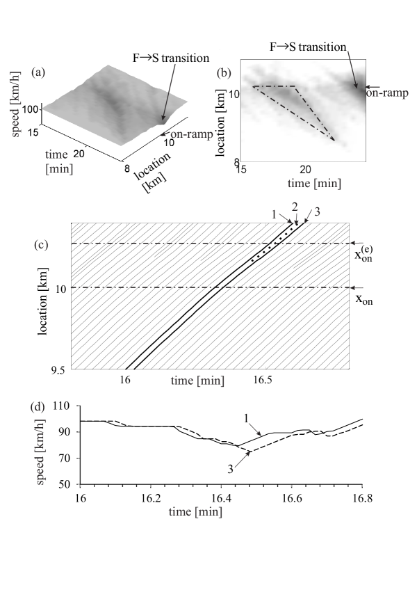
Figure 24: Simulations of dynamics of permanent speed disturbance at on-ramp bottleneck on single-lane road for traffic flow consisting only of manual driving vehicles related to Fig. 17 (c, d): (a, b) Speed in space and time (a) and the same data presented by regions with variable shades of gray (b) (in white regions the speed is equal to or higher than 105 km/h, in black regions the speed is smaller than 20 km/h); in (a, b), we show the same data as those in Fig. 17 (c, d), however, for smaller space and time intervals. (c) Fragment of vehicle trajectories in space and time related to (a, b). (d) Microscopic vehicle speeds along trajectories as time functions labeled by the same numbers as those in (c). In (b), dashed-dotted lines denote F$\rightarrow$S$\rightarrow$F transitions. $q_{\rm on}=$ 320 vehicles/h, $q_{\rm in}=$ 2000 vehicles/h.

To understand this negative effect of the ACC-vehicles on traffic flow, firstly note that as long as the percentage of the ACC-vehicles in a mixture traffic flow is not very large, traffic breakdown at the bottleneck is qualitatively the same time-delayed F$\rightarrow$S transition (Figs. 22 (a, b) and 23 (a, b)) as that in traffic flow consisting of manual driving vehicles only (Fig. 17 (c, d)). In both cases, WSPs result from the breakdown (Figs. 17 (c, d), 22 (a, b), and 23 (a, b)). Moreover, in both cases, before traffic breakdown occurs (time intervals $0<t<T^{\rm(B)}$ in Figs. 17 (c, d), 22 (a, b), and 23 (a, b)), there are many F$\rightarrow$S$\rightarrow$F transitions at the bottlenecks (dashed-dotted lines shown in Figs. 22 (d) and 24 (b) denote some of the regions of synchronized flow occurring due to a sequence of the F$\rightarrow$S$\rightarrow$F transitions). As explained in [544], the F$\rightarrow$S$\rightarrow$F transitions determine the dynamics of a permanent speed disturbance at the bottleneck.

A crucial difference between a mixture traffic flow and traffic flow without ACC-vehicles becomes clear, when we consider the dynamics of a permanent speed disturbance at the bottleneck: We have found that the amplitude of the permanent speed disturbance at the bottleneck occurring in the mixture traffic flow can increase considerably in comparison with that occurring in free flow consisting only of manual driving vehicles (Figs. 22 (c–f) and 24).

When a vehicle moving at a low speed in the on-ramp lane merges from the on-ramp to the main road (bold dotted trajectory 2 in Fig. 24 (c)) between two vehicles moving on the main road (bold trajectories 1 and 3 in Fig. 24 (c)), then, in comparison with vehicle 1 moving on the main road that is not influenced by the merging vehicle, vehicle 3 (bold trajectory 3 in Fig. 24 (c)) should decelerate to the speed of this merging vehicle. As a result, due to the vehicle merging the speed decreases within the permanent speed disturbance localized at the bottleneck (compare speeds of vehicles 1 and 3 in Fig. 24 (d)).

It turns out that the effect of the speed reduction caused by the merging vehicle can increase considerably, when vehicle 3 is an ACC-vehicle (bold dashed trajectory 3 in Fig. 22 (e)). Indeed, the deceleration of the ACC-vehicle (vehicle 3 in Fig. 22 (f)) due to the merging vehicle (bold dotted trajectory 2 in Fig. 22 (e)) becomes considerably larger than in the case of traffic flow without ACC-vehicles (compare speeds of vehicles 1 and 3 in Fig. 22 (f) with speeds of vehicles 1 and 3 in Fig. 24 (d), respectively). Due to a stronger speed reduction at the bottleneck caused by the ACC-vehicles, the probability of traffic breakdown increases at the same flow rates as those in the case of traffic flow consisting of manual driving vehicles only (Fig. 21 (a)).

When the percentage $\gamma$ of the ACC-vehicles increases, the frequency of large speed disturbances at the bottleneck caused by the ACC-vehicles increases either. This explains why at given flow rates the probability of traffic breakdown increases when $\gamma$ increases from $\gamma\approx 5\%$ to $\gamma^{\rm(increase)}_{\rm cr}$ (the value $\gamma^{\rm(increase)}_{\rm cr}\approx 30\%$ for parameters of ACC-vehicles used in Fig. 21 (b)). Only when the percentage of the ACC-vehicles $\gamma>\gamma^{\rm(increase)}_{\rm cr}$, long stable platoons of the ACC-vehicle can occur that lead to a decrease in the breakdown probability. Indeed, free flow consisting of $100\%$ ACC-vehicles is stable.

To understand the physics of the deterioration of the performance of the traffic system through the ACC-vehicles in more details, we should note that in accordance with the hypothesis of the three-phase theory about the existence of 2D-states of traffic flow [200, 201, 216, 217, 218, 219, 220, 221, 222, 223, 224, 225, 226, 227, 228, 229, 230], drivers do not control the space gap $g$ to the preceding vehicle when condition

$$g_{\rm safe}\leq g\leq G,$$ (32)

is satisfied, where $G$ and $g_{\rm safe}$ are the synchronization and safe space gaps, respectively.

In contrast to the manual driver behavior (32), in accordance with the classical ACC-model (21), the ACC-vehicle tries to reach an $``$optimal” space gap given by formula (25). This qualitative different dynamic behavior of the ACC-vehicles and manual driving vehicles could explain the occurrence of large disturbances in free flow at the bottleneck. When the space gap between the ACC-vehicle and the merging manual vehicle is smaller than that given by formula (25), the ACC-vehicle decelerates, whereas a manual driving vehicle should not decelerate as long as condition (32) is satisfied. The deceleration of the ACC-vehicle is the stronger, the larger the coefficient $K_{1}$ in (21). This can explain the result of simulations that the larger the coefficient $K_{1}$, the more is the shift of the function $P^{\rm(B)}(q_{\rm sum})$ to the left in the flow rate-axis (curves 1–4 in Fig. 21 (a)). We can make the following conclusion.

• When dynamics rules of motion of automatic driving vehicles differ considerably from those of human driving vehicles, such automatic driving vehicles can cause the deterioration of the performance of the traffic system. In particular, speed disturbances in a mixture traffic flow at road bottlenecks can increase strongly. This can cause the considerable increase in the probability of traffic breakdown.

Naturally, through the use of cooperative driving (Sec. 2.5) this negative effect of automatic driving vehicles on traffic flow could be reduced. However, it seems better to develop such dynamics rules of motion of automatic driving vehicles that avoid situations at which human drivers can consider automatic driving vehicles as $``$obstacles”.

6 Automatic driving vehicles learning from driver behavior in real traffic: ACC in framework of three-phase theory

The deterioration of the performance of the traffic system through the ACC-vehicles discussed in Sec. 5 could be avoided through the use of automatic driving systems in vehicles, which learn from behaviors of drivers in real traffic as incorporated in hypotheses of the three-phase theory.

In particular, in accordance with the hypothesis of three-phase theory about 2D-states of traffic flow [200, 201, 216, 217, 218, 219, 220, 221, 222, 223, 224, 225, 226, 227, 228, 229, 230], we have introduced ACC-systems [644, 645, 646], in which, in contrast with the classical model of the ACC-vehicle (20), there is no fixed desired time headway of ACC-vehicle to the preceding vehicle.

In these ACC-systems based on the three-phase theory [644, 645, 646], when the space gap to the preceding vehicle is within a 2D-region in the space-gap–speed plane (dashed region in Fig. 25), i.e., condition (32) is satisfied, then the acceleration (deceleration) of an ACC-vehicle is given by formula

$$a(t)=K_{\rm\Delta v}\Delta v(t).$$ (33)

This means that the ACC-vehicle adapts its speed to the speed of the preceding vehicle without caring, what the precise space gap (time headway) is. In (33), $K_{\rm\Delta v}$ is a dynamic coefficient ($K_{\rm\Delta v}>0$). At $g>G$ the ACC-vehicle accelerates, whereas at $g<g_{\rm safe}$ the ACC-vehicle decelerates. Outside of the 2D-region in the space-gap–speed plane (Fig. 25) formula (33) is not applied [646, 647, 648, 649].

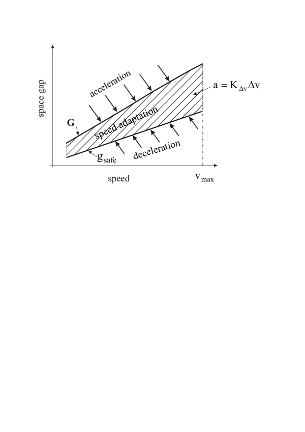
Figure 25: Explanation of ACC in the framework of three-phase theory [644, 645, 646]: A part of 2D-states of traffic flow in the space-gap–speed plane (dashed region) within which an ACC-vehicle moves in accordance with Eq. (33).

Thus, in some traffic situations acceleration (deceleration) of the ACC-vehicle does not depend on the space gap, i.e., on the time headway to the preceding vehicle at all. In other words, the ACC mode (33) does not maintain some desired time headway of the classical model of the ACC-vehicle (20). Moreover, the dynamic coefficient $K_{\rm\Delta v}$ in (33) can be chosen to be considerably smaller than the dynamic coefficient $K_{2}$ in the classical model of the ACC-vehicle (20). This explains the following possible advantages of the ACC-system based on three-phase theory in comparison with the classical ACC-system (20):

• The removing of a conflict between the dynamic and comfortable ACC behavior. In particular, a much comfortable vehicle motion is possible.

• The reduction of fuel consumption and $\rm CO_{2}$ emissions while moving in congested traffic.

• Because the ACC-mode (33) decreases speed changes in traffic flow, a sequence of such ACC-vehicles can prevent traffic breakdown at a bottleneck.

Therefore, a development of automatic driving vehicles based on the three-phase theory can be a very interesting task for further investigations.

7 Conclusions

(i) The empirical metastability of free flow with respect to the F$\rightarrow$S transition (traffic breakdown) at a highway bottleneck can be considered the empirical fundament of transportation science.

(ii) The theoretical fundament of transportation science resulting from the above empirical fundament is as follows: At any time instant, there are the infinite number of highway capacities within a range of the flow rate between the minimum capacity and the maximum capacity; within this flow rate range, traffic breakdown can be induced at the bottleneck.

(iii) Additionally to the minimum capacity and the maximum capacity, an important characteristic of traffic breakdown is a threshold flow rate for spontaneous traffic breakdown at a bottleneck.

(iv) Classical traffic and transportation theories failed to explain the empirical evidence that traffic breakdown at the bottleneck is an F$\rightarrow$S transition occurring in metastable free flow at the bottleneck. For this reasons, traffic flow models, which are based on these classical traffic theories, cannot be used for a reliable analysis of the impact of automatic driving and/or other ITS-applications on traffic flow. Simulations of the effect of automatic driving and/or other ITS-applications on traffic flow with the use of such traffic simulation models and tools lead to incorrect results and invalid conclusions.

(v) To perform reliable analysis of the impact of automatic driving and/or other ITS-applications on traffic flow, traffic flow models in the framework of the three-phase theory should be used. This is because these models can explain the empirical evidence that traffic breakdown at the bottleneck is an F$\rightarrow$S transition occurring in metastable free flow at the bottleneck.

(vi) Based on simulations with a stochastic three-phase traffic flow model we have found that depending on the parameters of automatic driving vehicles, they can either decrease or increase the probability of traffic breakdown in a mixture traffic flow consisting of a random distribution of automatic driving and manual driving vehicles. The increase in the probability of traffic breakdown at a bottleneck, i.e., the deterioration of the performance of the traffic system can occur already at a small percentage (about 5$\%$) of automatic driving vehicles. The negative effect of the automatic driving vehicles on traffic flow can be realized, even if any platoon of the automatic driving vehicles satisfies condition for string stability; this effect occurs even at the same flow rates at the bottleneck at which there is no traffic breakdown in free flow consisting of 100$\%$ of automatic driving vehicles.

Appendix A Kerner-Klenov stochastic microscopic model in framework of three-phase traffic theory

In a discrete model version of Kerner-Klenov stochastic microscopic three-phase model [526] used for simulations in Secs. 4 and 5, rather than the continuum space co-ordinate of [520, 525], a discrete space co-ordinate with a small enough value of the discrete cell $\delta x=0.01$ m is used. Consequently, the vehicle speed and acceleration (deceleration) discretization intervals are $\delta v$= $\delta x/\tau$ and $\delta a$= $\delta v/\tau$, respectively, where time step $\tau=$ 1 s. Because in the discrete model version discrete (and dimensionless) values of speed and acceleration are used, which are measured respectively in values $\delta v$ and $\delta a$, and time is measured in values of $\tau$, value $\tau$ in all formulas below is assumed to be the dimensionless value $\tau=1$.

A.1 Update rules of vehicle motion in road lane

Update rules of vehicle motion are as follows [520, 525, 526]:

$$v_{n+1}=\max(0,\min({v_{\rm free},\tilde{v}_{n+1}+\xi_{n},v_{n}+a\tau,v_{{\rm s},n}})),$$ (34)

$$x_{n+1}=x_{n}+v_{n+1}\tau,$$ (35)

where the index $n$ corresponds to the discrete time $t_{\rm n}=\tau n,\ n=0,1,...$, $v_{n}$ is the vehicle speed at time step $n$, $a$ is the maximum acceleration, $\tilde{v}_{n}$ is the vehicle speed without speed fluctuations $\xi_{n}$:

$$\tilde{v}_{n+1}=\min(v_{\rm free},v_{{\rm s},n},v_{{\rm c},n}),$$ (36)

$$v_{{\rm c},n}=\left\{\begin{array}[]{ll}v_{n}+\Delta_{n}&\textrm{at $g_{n}\leq G_{n}$,}\\ v_{n}+a_{n}\tau&\textrm{at $g_{n}>G_{n}$},\\ \end{array}\right.$$ (37)

$$\Delta_{n}=\max(-b_{n}\tau,\min(a_{n}\tau,\ v_{\ell,n}-v_{n})),$$ (38)

$$g_{n}=x_{\ell,n}-x_{n}-d,$$ (39)

the subscript $\ell$ denotes variables related to the preceding vehicle, $v_{{\rm s},n}$ is a safe speed at time step $n$, $v_{\rm free}$ is the maximum speed in free flow, $\xi_{n}$ describes speed fluctuations; $v_{{\rm c},n}$ is a desired speed; all vehicles have the same length $d$. The vehicle length $d$ includes the mean space gap between vehicles within a wide moving jam where the speed is zero. Values $a_{n}\geq 0$ and $b_{n}\geq 0$ in (37), (38) restrict changes in speed per time step when the vehicle accelerates or adjusts the speed to that of the preceding vehicle.

A.2 Synchronization gap and hypothetical steady states of synchronized flow

Equations (37), (38) describe the adaptation of the vehicle speed to the speed of the preceding vehicle, i.e., the speed adaptation effect in synchronized flow. This vehicle speed adaptation takes place within the synchronization gap $G_{n}$: At

$$g_{n}\leq G_{n}$$ (40)

the vehicle tends to adjust its speed to the preceding vehicle. This means that the vehicle decelerates if $v_{n}>v_{\ell,n}$, and accelerates if $v_{n}<v_{\ell,n}$ [520].

In the general rules (34)–(38), the synchronization gap $G_{n}$ depends on the vehicle speed $v_{n}$ and on the speed of the preceding vehicle $v_{\ell,n}$:

$$G_{n}=G(v_{n},v_{\ell,n}),$$ (41)

$$G(u,w)=\max(0,\lfloor k\tau u+a^{-1}u(u-w)\rfloor),$$ (42)

$k>1$ is constant.

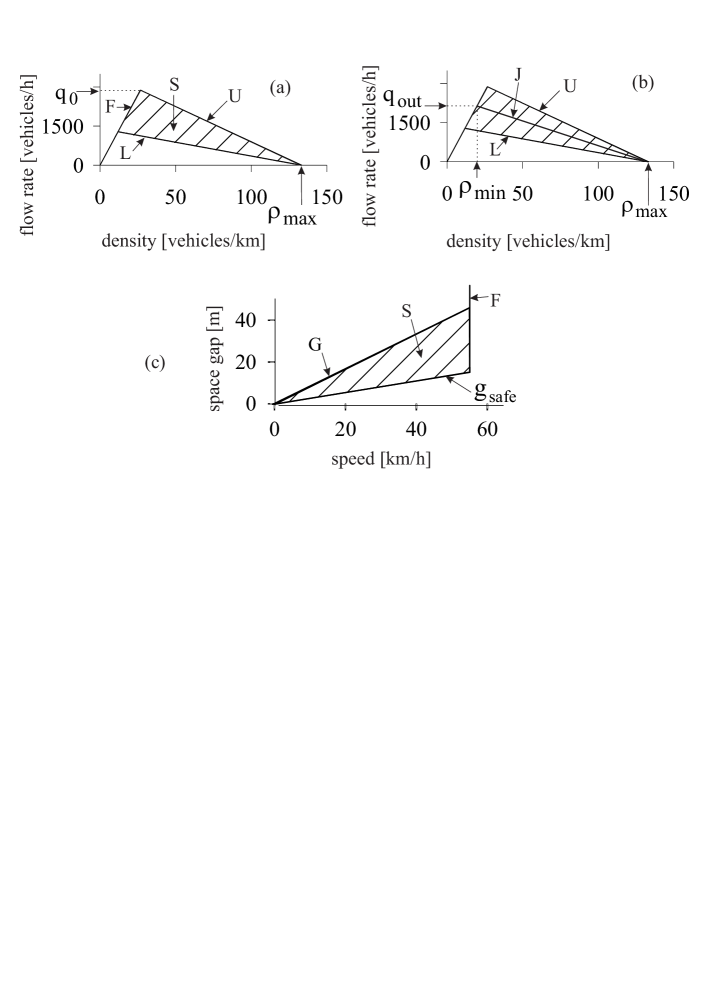
Figure 26: Steady speed states for the three-phase traffic flow model in the flow–density (a, b) and in the space-gap–speed planes (c). $L$ and $U$ are, respectively, lower and upper boundaries of 2D-regions of steady states of synchronized flow, $F$ - free flow, $S$ – synchronized flow, $J$ is line $J$ whose slope is equal to the characteristic mean velocity $v_{\rm g}$ of a wide moving jam; in the flow–density plane, the line $J$ represents the propagation of the downstream front of the wide moving jam with time-independent velocity $v_{\rm g}$.

The speed adaptation effect within the synchronization gap is related to the hypothesis of three-phase theory about 2D-states of traffic flow

[200, 201, 216, 217, 218, 219, 220, 221, 222],

[223, 224, 225, 226, 227, 228, 229, 230]. Respectively, as for the continuum-in-space Kerner-Klenov model (see Sec. 16.3 of the book [200]), for the discrete model considered here hypothetical steady states of traffic flow cover a 2D-region in the flow–density plane (Fig. 26 (a)). However, because the speed $v$ and space gap $g$ are integer in the discrete model, the steady states do not form a continuum in the flow–density plane as they do in the continuum model. The inequalities

$$g\leq G(v,\ v)\quad\rm{and}\quad v\leq\rm{min}(v_{\rm free},\ v_{\rm s}(g,\ v))$$ (43)

define a 2D-region in the flow–density plane in which the hypothetical steady states of traffic flow exist for the discrete model, when all model fluctuations are neglected. In (43), we have taken into account that in the hypothetical 2D-steady states of traffic flow vehicle speeds are assumed to be time-independent and the speed of each of the vehicles is equal to the speed of the associated preceding vehicle: $v=v_{\ell}$.

It should be emphasized that due to model fluctuations (see Sec. A.3), 2D-steady states of traffic flow are destroyed, i.e., they do not exist in simulations. This explains the term $``$hypothetical” 2D-steady states of traffic flow. Rather than 2D-steady states of traffic flow, in the Kerner-Klenov stochastic model all 2D-states of traffic flow are non-homogeneous in space and time. However, in accordance with the three-phase theory (see explanations in Secs. 4.3.4 and 6.3.3 of the book [200]), the non-homogeneous in space and time 2D-states of traffic flow of the Kerner-Klenov stochastic model exhibit qualitatively the same features with respect to phase transitions (F$\rightarrow$S, S$\rightarrow$F, and S$\rightarrow$J transitions) as those postulated in the three-phase theory for 2D-steady states of traffic flow [200, 201, 216, 217, 218, 219, 220, 221, 222], [223, 224, 225, 226, 227, 228, 229, 230].

A.3 Model speed fluctuations

In the model, random deceleration and acceleration are applied depending on whether the vehicle decelerates or accelerates, or else maintains its speed:

$$\xi_{n}=\left\{\begin{array}[]{ll}\xi_{\rm a}&\textrm{if $S_{n+1}=1$}\\ -\xi_{\rm b}&\textrm{if $S_{n+1}=-1$}\\ \xi^{(0)}&\textrm{if $S_{n+1}=0$}.\end{array}\right.$$ (44)

State of vehicle motion $S$ in (44) is determined by formula

$$S_{n+1}=\left\{\begin{array}[]{ll}-1&\textrm{if $\tilde{v}_{n+1}<v_{n}$}\\ 1&\textrm{if $\tilde{v}_{n+1}>v_{n}$}\\ 0&\textrm{if $\tilde{v}_{n+1}=v_{n}$}.\end{array}\right.$$ (45)

In (44), $\xi_{\rm b}$, $\xi^{(0)}$, and $\xi_{\rm a}$ are random sources for deceleration and acceleration that are as follows:

$$\xi_{\rm b}=a^{(\rm b)}\tau\Theta(p_{\rm b}-r),$$ (46)

$$\xi^{(0)}=a^{(0)}\tau\left\{\begin{array}[]{ll}-1&\textrm{if $r<p^{(0)}$}\\ 1&\textrm{if $p^{(0)}\leq r<2p^{(0)}$}\quad{\rm and}\ v_{n}>0\\ 0&\textrm{otherwise},\end{array}\right.$$ (47)

$$\xi_{\rm a}=a^{(\rm a)}\tau\Theta(p_{\rm a}-r),$$ (48)

$p_{\rm b}$ is probability of random deceleration, $p_{\rm a}$ is probability of random acceleration, $p^{(0)}$ and $a^{(0)}\leq a$ are constants, $a^{(\rm a)}=a^{(\rm b)}=a$, $r={\rm rand(0,1)}$, $\Theta(z)=0$ at $z<0$ and $\Theta(z)=1$ at $z\geq 0$.

A.4 Stochastic time delays in vehicle acceleration and deceleration

To simulate time delays either in vehicle acceleration or in vehicle deceleration, $a_{n}$ and $b_{n}$ in (38) are taken as the following stochastic functions

$$a_{n}=a\Theta(P_{\rm 0}-r_{\rm 1}),$$ (49)

$$b_{n}=a\Theta(P_{\rm 1}-r_{\rm 1}),$$ (50)

$$P_{\rm 0}=\left\{\begin{array}[]{ll}p_{\rm 0}&\textrm{if $S_{n}\neq 1$}\\ 1&\textrm{if $S_{n}=1$},\end{array}\right.$$ (51)

$$P_{\rm 1}=\left\{\begin{array}[]{ll}p_{\rm 1}&\textrm{if $S_{n}\neq-1$}\\ p_{\rm 2}&\textrm{if $S_{n}=-1$},\end{array}\right.$$ (52)

$r_{1}={\rm rand}(0,1)$, $p_{\rm 1}$ is constant, $p_{\rm 0}=p_{\rm 0}(v_{n})$ and $p_{\rm 2}=p_{\rm 2}(v_{n})$ are speed functions.

The physical sense of the functions $P_{0}$ and $P_{1}$ in (51) and (52) is as follows. The function $P_{0}$ in (51) determines the probability $\psi_{\rm a}$ of a random time delay in vehicle acceleration at time step $n+1$ corresponding to

$$\psi_{\rm a}=1-P_{0}.$$ (53)

The function $P_{1}$ (52) determines the probability $\psi_{\rm b}$ of a random time delay in vehicle deceleration at time step $n+1$ corresponding to

$$\psi_{\rm b}=1-P_{1}.$$ (54)

A.5 Safe speed

In the model, the safe speed $v_{{\rm s},n}$ in (34) is chosen in the form

$$v_{{\rm s},n}=\min{(v^{\rm(safe)}_{n},g_{n}/\tau+v^{\rm(a)}_{\ell})},$$ (55)

$v^{\rm(a)}_{\ell}$ is an $``$anticipation” speed of the preceding vehicle that will be considered below, the function

$$v^{\rm(safe)}_{n}=\lfloor v^{\rm(safe)}(g_{n},\ v_{\ell,n})\rfloor$$ (56)

in (55) is related to the safe speed $v^{\rm(safe)}(g_{n},\ v_{\ell,n})$ in the model by Krauß et al. [273, 274], which is a solution of the Gipps’s equation [271]

$$v^{\rm(safe)}\tau_{\rm safe}+X_{\rm d}(v^{\rm(safe)})=g_{n}+X_{\rm d}(v_{\ell,n}),$$ (57)

where $\tau_{\rm safe}$ is a safe time gap that can be individual for drivers, $X_{\rm d}(u)$ is the braking distance that should be passed by the vehicle moving first with the speed $u$ before the vehicle can come to a stop:

$$X_{\rm d}(u)=b\tau^{2}\bigg{(}\alpha\beta+\frac{\alpha(\alpha-1)}{2}\bigg{)},$$ (58)

$\alpha=\lfloor u/b\tau\rfloor$ and $\beta=u/b\tau-\alpha$ are the integer and fractional parts of $u/b\tau$, respectively, $b$ is constant.

The safe speed $v^{\rm(safe)}$ as a solution of equation (57) at the distance $X_{\rm d}(u)$ given by (58) and at $\tau_{\rm safe}=\tau$ has been found in [273, 274]

$$v^{\rm(safe)}(g_{n},v_{\ell,n})=b\tau(\alpha_{\rm safe}+\beta_{\rm safe}),$$ (59)

where

$$\alpha_{\rm safe}=\lfloor{\sqrt{2\frac{X_{\rm d}(v_{\ell,n})+g_{n}}{b\tau^{2}}+\frac{1}{4}}-\frac{1}{2}}\rfloor,$$ (60)

$$\beta_{\rm safe}=\frac{X_{\rm d}(v_{\ell,n})+g_{n}}{(\alpha_{\rm safe}+1)b\tau^{2}}-\frac{\alpha_{\rm safe}}{2}.$$ (61)

The safe speed in the model by Krauß et al. [273, 274] provides collision-less motion of vehicles if the time gap $g_{n}/v_{n}$ between two vehicles is greater than or equal to the time step $\tau$, i.e., if $g_{n}\geq v_{n}\tau$ [274]. In the model, it is assumed that in some cases, mainly due to lane changing or merging of vehicles onto the main road within the merging region of bottlenecks, the space gap $g_{n}$ can become less than $v_{n}\tau$. In these critical situations, the collision-less motion of vehicles in the model is a result of the second term in (55) in which some prediction ($v^{\rm(a)}_{\ell}$) of the speed of the preceding vehicle at the next time step is used. The related $``$anticipation” speed $v^{\rm(a)}_{\ell}$ at the next time step that is given by formula

$$v^{\rm(a)}_{\ell}=\max(0,\min(v^{\rm(safe)}_{\ell,n},v_{\ell,n},g_{\ell,n}/\tau)-a\tau),$$ (62)

where $v^{\rm(safe)}_{\ell,n}$ is the safe speed (56), (59)–(61) for the preceding vehicle, $g_{\ell,n}$ is the space gap in front of the preceding vehicle. Simulations have shown that formulas (55), (56), (59)–(62) lead to collision-less vehicle motion over a wide range of parameters of the merging region of the bottleneck.

A.6 Boundary and initial conditions

In the model, open boundary conditions are applied. At the beginning of the road new vehicles are generated one after another in each of the lanes of the road at time moments

$$t^{(k)}=\tau\lceil k\tau_{\rm in}/\tau\rceil,\ k=1,2,....$$ (63)

In (63), $\tau_{\rm in}=1/q_{\rm in}$, $q_{\rm in}$ is the flow rate in the incoming boundary flow per lane, $\lceil z\rceil$ denotes the nearest integer greater than or equal to $z$. A new vehicle appears on the road only if the distance from the beginning of the road ($x=x_{\rm b}$) to the position $x=x_{\ell,n}$ of the farthest upstream vehicle on the road is not smaller than the distance

$$x_{\ell,n}-x_{\rm b}\geq v_{\ell,n}\tau+d,$$ (64)

where $n=t^{(k)}/\tau$. Otherwise, condition (64) is checked at time $(n+1)\tau$ that is the next one to time $t^{(k)}$ (63), and so on, until the condition (64) is satisfied. Then the next vehicle appears on the road. After this occurs, the number $k$ in (63) is increased by 1.

The speed $v_{n}$ and coordinate $x_{n}$ of the new vehicle are

$$\begin{array}[]{ll}v_{n}=v_{\ell,n},\\ x_{n}={\rm max}(x_{\rm b},x_{\ell,n}-\lfloor{v_{n}\tau_{\rm in}}\rfloor).\end{array}$$ (67)

The flow rate $q_{\rm in}$ is chosen to have the value $v_{\rm free}\tau_{\rm in}$ integer. In the initial state ($n=0$), all vehicles have the maximum speed $v_{n}=v_{\rm free}$ and they are positioned at space intervals $x_{\ell,n}-x_{n}=v_{\rm free}\tau_{\rm in}$.

After a vehicle has reached the end of the road it is removed. Before this occurs, the farthest downstream vehicle maintains its speed. For the vehicle following the farthest downstream one, the $``$anticipation” speed $v^{\rm(a)}_{\ell}$ in (62) is equal to the speed of the farthest downstream vehicle.

A.7 Model of on-ramp bottleneck

Figure 27: Model of on-ramp bottleneck on single-lane road.

The on-ramp bottleneck consists of two parts (Fig. 27):

(i)

The merging region of length $L_{\rm m}$ where vehicle can merge onto the main road from the on-ramp lane.

(ii)

A part of the on-ramp lane of length $L_{\rm r}$ upstream of the merging region where vehicles move in accordance with the model (34)–(39). The maximal speed of vehicles is $v_{\rm free}=v_{\rm free\ on}$.

At the beginning of the merging region of the on-ramp lane ($x=x^{\rm(b)}_{\rm on}$) the flow rate to the on-ramp $q_{\rm on}$ is given as in $q_{\rm in}$.

A.8 Manual driving vehicle merging at on-ramp bottleneck

A merging region at an on-ramp bottleneck is a road region of length $L_{\rm m}$ within which a vehicle moving in the on-ramp lane merges to the right lane of the main road (Fig. 27). When a vehicle is within the merging region of the bottleneck, the vehicle takes into account the space gaps to the preceding vehicles and their speed both in the current and target lanes. Respectively, instead of formula (37), in (36) for the speed $v_{{\rm c},n}$ the following formula is used:

$$v_{{\rm c},n}=\left\{\begin{array}[]{ll}v_{n}+\Delta^{+}_{n}&\textrm{at $g^{+}_{n}\leq G(v_{n},\hat{v}^{+}_{n})$,}\\ v_{n}+a_{n}\tau&\textrm{at $g^{+}_{n}>G(v_{n},\hat{v}^{+}_{n})$},\\ \end{array}\right.$$ (68)

$$\Delta^{+}_{n}=\max(-b_{n}\tau,\min(a_{n}\tau,\ \hat{v}^{+}_{n}-v_{n})),$$ (69)

$$\hat{v}^{+}_{n}=\max(0,\min(v_{\rm free},\ v^{+}_{n}+\Delta v^{(2)}_{r})),$$ (70)

$\Delta v^{(2)}_{r}$ is constant. Superscripts $+$ and $-$ in variables, parameters, and functions denote the preceding vehicle and the trailing vehicle in the $``$target” (neighboring) lane, respectively (the target lane is the lane into which the vehicle wants to change).

The safe speed $v_{{\rm s},n}$ in (34), (36) for the vehicle that is the closest one to the end of merging region is chosen in the form

$$v_{{\rm s},n}=\lfloor v^{\rm(safe)}(x^{\rm(e)}_{\rm on}-x_{n},\ 0)\rfloor.$$ (71)

Vehicle merging at the bottleneck occurs, when safety conditions ($\ast$) or safety conditions ($\ast\ast$) are satisfied. Safety conditions ($\ast$) are as follows:

$$\begin{array}[]{ll}g^{+}_{n}>\min(\hat{v}_{n}\tau,\ G(\hat{v}_{n},v^{+}_{n})),\\ g^{-}_{n}>\min(v^{-}_{n}\tau,\ G(v^{-}_{n},\hat{v}_{n})),\end{array}$$ (72)

$$\hat{v}_{n}=\min(v^{+}_{n},\ v_{n}+\Delta v^{(1)}_{r}),$$ (73)

$\Delta v^{(1)}_{r}>0$ is constant.

Safety conditions ($\ast\ast$) are as follows:

$$x^{+}_{n}-x^{-}_{n}-d>g^{\rm(min)}_{\rm target},$$ (74)

where

$$g^{\rm(min)}_{\rm target}=\lfloor\lambda_{\rm b}v^{+}_{n}+d\rfloor,$$ (75)

$\lambda_{\rm b}$ is constant. In addition to conditions (74), the safety condition ($\ast\ast$) includes the condition that the vehicle should pass the midpoint

$$x^{\rm(m)}_{n}=\lfloor(x^{+}_{n}+x^{-}_{n})/2\rfloor$$ (76)

between two neighboring vehicles in the target lane, i.e., conditions

$$\begin{array}[]{ll}x_{n-1}<x^{\rm(m)}_{n-1}\ \textrm{and}\ x_{n}\geq x^{\rm(m)}_{n}\\ \ \textrm{\it or}\\ x_{n-1}\geq x^{\rm(m)}_{n-1}\ \textrm{and}\ x_{n}<x^{\rm(m)}_{n}.\end{array}$$ (77)

should also be satisfied.

The vehicle speed after vehicle merging is equal to

$$v_{n}=\hat{v}_{n}.$$ (78)

Under conditions ($\ast$), the vehicle coordinate $x_{n}$ remains the same. Under conditions ($\ast\ast$), the vehicle coordinate $x_{n}$ is equal to

$$x_{n}=x^{\rm(m)}_{n}.$$ (79)

A.9 ACC-vehicle merging at on-ramp bottleneck

In the on-ramp lane, an ACC vehicle moves in accordance with the model (21), (27), (28). The maximal speed of the ACC vehicle in the on-ramp lane is $v_{\rm free}=v_{\rm free\ on}$. The safe speed $v_{{\rm s},n}$ in (28) for the ACC vehicle that is the closest one to the end of merging region is the same as that for manual driving vehicles (71).

ACC-vehicle merges from the on-ramp lane onto the main road, when some ACC-safety conditions ($\ast$) or safety conditions ($\ast\ast$) are satisfied. Safety conditions ($\ast$) for ACC-vehicles are as follows:

$$\begin{array}[]{ll}g^{+}_{n}>\hat{v}_{n}\tau,\quad g^{-}_{n}>v^{-}_{n}\tau,\end{array}$$ (80)

where $\hat{v}_{n}$ is given by formula (73). Safety conditions ($\ast\ast$) are given by formulas (74)–(77), i.e., they are the same as those for manual driving vehicles. Respectively, as for manual driving vehicles, the ACC-vehicle speed and its coordinate after ACC-vehicle merging are determined by formulas (78) and (79).

Table 1: Model parameters used in simulations (other model parameters are given in figure captions)

Vehicle motion in road lane:

$\tau_{\rm safe}=\tau$, $\tau=$1 s, $d=7.5\ \rm m/\delta x$, $\delta x=$ 0.01 m,

$v_{\rm free}=30\ {\rm ms^{-1}}/\delta v$, $b=1\ {\rm ms^{-2}}/\delta a$,

$\delta v=0.01\ {\rm ms^{-1}}$,  $\delta a=0.01\ {\rm ms^{-2}}$, $k=$ 3,

$p_{1}=$ 0.3, $p_{b}=0.1$, $p_{a}=0.17$,

$p^{(0)}=0.005$, $p_{\rm 2}(v_{n})=0.48+0.32\Theta{(v_{n}-v_{21})}$,

$p_{\rm 0}(v_{n})=0.575+0.125\min{(1,v_{n}/v_{01})}$,

$a^{(0)}=0.2a$, $a^{(\rm a)}=a^{(\rm b)}=a$,

$v_{01}=10\ {\rm ms^{-1}}/\delta v$, $v_{21}=15\ {\rm ms^{-1}}/\delta v$, $a=$ 0.5 ${\rm ms^{-2}}/\delta a$.

Model of on-ramp bottleneck:

$\lambda_{\rm b}=$ 0.75,  $v_{\rm free\ on}=22.2\ {\rm ms^{-1}}/\delta v$,

$\Delta v^{\rm(2)}_{\rm r}=$ 5 ${\rm ms^{-1}}/\delta v$,

$L_{\rm r}=1\ {\rm km}/\delta x$, $\Delta v^{\rm(1)}_{\rm r}=10\ {\rm ms^{-1}}/\delta v$,

$L_{\rm m}=$ 0.3  ${\rm km}/\delta x$.

Acknowledgments:

I thank our partners for their support in the project $``$UR:BAN - Urbaner Raum: Benutzergerechte Assistenzsysteme und Netzmanagement”, funded by the German Federal Ministry of Economics and Technology by resolution of the German Federal Parliament. I thank Sergey Klenov for very helpful suggestions and help in simulations.

References

- [1] B.D. Greenshields, in Highway Research Board Proceedings 14 (1935) 448–477.
- [2] A.D. May, Traffic Flow Fundamentals, Prentice-Hall, Inc., New Jersey, 1990.
- [3] Highway Capacity Manual 2000, National Research Council, Transportation Research Boad, Washington, D.C., 2000.
- [4] Highway Capacity Manual 2010, National Research Council, Transportation Research Boad, Washington, D.C., 2010.
- [5] F.L. Hall, M.A. Gunter, Trans. Res. Rec. 1091 (1986) 1–9.
- [6] F.L. Hall, Trans. Res. A 21 (1987) 191–201.
- [7] F.L. Hall, K. Agyemang-Duah, Trans. Res. Rec. 1320 (1991) 91–98.
- [8] F.L. Hall, V.F. Hurdle, J.H. Banks, Transp. Res. Rec. 1365 (1992) 12–18.
- [9] L. Elefteriadou, R.P. Roess, W.R. McShane, Transp. Res. Rec. 1484 (1995) 80–89.
- [10] B.N. Persaud, S. Yagar, R. Brownlee, Trans. Res. Rec. 1634 (1998) 64–69.
- [11] M. Lorenz, L. Elefteriadou, Transp. Res. Circular E-C018 (2000) 84–95.
- [12] W. Brilon, M. Regler, J. Geistefeld, Straßenverkehrstechnik, Heft 3 (2005) 136.
- [13] W. Brilon, H. Zurlinden, Straßenverkehrstechnik, Heft 4 (2004) 164.
- [14] W. Brilon, J. Geistefeldt, M. Regler, in: [185] (2005) pp. 125–144.
- [15] J. Geistefeldt, W. Brilon, in: [187] (2009) pp. 583–602.
- [16] L. Elefteriadou, A. Kondyli, W. Brilon, F.L. Hall, B. Persaud, S. Washburn, J. of Transp. Eng. 140 (4) (2014).
- [17] L. Elefteriadou, An Introduction to Traffic Flow Theory. Springer Optimization and Its Applications, Vol. 84, Springer, Berlin 2014).
- [18] A. Ceder, Investigation of Two-Regime Traffic Flow Models at the Micro- and Macroscopic Levels, Ph.D. Thesis, UC, Berkeley University, Berkeley, CA, 1975.
- [19] A. Ceder, A.D. May, Transp. Res. Rec. 567 (1976) 1–15.
- [20] F.L. Hall, D. Barrow, Transp. Res. Rec. 1194 (1988) 55–65.
- [21] F.L. Hall, W. Brilon, Transp. Res. Rec. 1457 (1994) 35–42.
- [22] F.L. Hall, A. Pushkar, Y. Shi, Transp. Res. Rec. 1398 (1993) 24–30.
- [23] A.D. May, Highway Res. Rec. 59 (1964) 9–38.
- [24] A.D. May, P. Athol, W. Parker, J.B. Rudden, Highway Res. Rec. 21 (1963) 48–70.
- [25] J. Drake, J. Shofer, A.D. May, Highway Res. Rec. 154 (1967) 53–87.
- [26] M.J. Cassidy, A. Skabardonis, A.D. May, Transp. Res. Rec. 1225 (1989) 61–72.
- [27] H.C. Chin, A.D. May, Transp. Res. Rec. 1320 (1991) 75–82.
- [28] J. Schoen, A.D. May, W. Reilly, T. Urbanik, Speed–Flow Relationships for Basic Freeway Segments, Final Report, NCHRP Project 3–45, JHK & Associates and Texas Transportation Institute, 1995.
- [29] B.N. Persaud, Study of a Freeway Bottleneck to Explore Some Unresolved Traffic Flow Issues, Ph.D. Dissertation, University of Toronto, Toronto, Canada, 1986.
- [30] B.N. Persaud, F.L. Hall, Trans. Res. A 23 (1989) 103–113.
- [31] B.N. Persaud, F.L. Hall, L.M. Hall, Transp. Res. Rec. 1287 (1990) 167–175.
- [32] B.N. Persaud, V.F. Hurdle, Transp. Res. Rec. 1194 (1988) 191–198.
- [33] B.N. Persaud, V.F. Hurdle, in: Proceedings of International Symposium on Highway Capacity, Karlsruhe, Germany, 1991.
- [34] B.N. Persaud, S. Yagar, D. Tsui, H. Look, Transp. Res. Rec. 1748 (2001) 110–115.
- [35] J. Ringert, T. Urbanik II, Transp. Res. Rec. 1398 (1993) 31–41.
- [36] J.H. Banks, Transp. Res. Rec. 1510 (1995) 1–10.
- [37] J.H. Banks, Transp. Res. Rec. 1225 (1989) 53–60.
- [38] J.H. Banks, Transp. Res. Rec. 1287 (1990) 20–28.
- [39] J.H. Banks, Evaluation of the Two-Capacity Phenomenon as a Basis for Ramp Metering, Final Report, Civil Engineering Report Series 9002, San Diego State University, San Diego, CA, 1990.
- [40] J.H. Banks, Transp. Res. Rec. 1320 (1991) 234–241.
- [41] J.H. Banks, Transp. Res. Rec. 1320 (1991) 83–90.
- [42] J.H. Banks, Transp. Res. Rec. 1394 (1993) 17–25.
- [43] J.H. Banks, Transp. Res. Rec. 1678 (1999) 128–134.
- [44] J.H. Banks, Transp. Res. Rec. 1802 (2002) 225–232.
- [45] P. Hsu, J.H. Banks, Transp. Res. Rec. 1398 (1993) 17–23.
- [46] S.M. Easa, A.D. May, Transp. Res. Rec. 772 (1980) 24–37.
- [47] L.C. Edie, Oper. Res. 9 (1961) 66–77.
- [48] L.C. Edie, E. Baverez, in: Third Int. Sym. on the Theory of Traffic Flow, 1995, pp. 26–37.
- [49] L.C. Edie, R.S. Foote, in: Highway Research Board Proceedings, HRB, National Research Council, Washington, D.C., 1958, 37, pp. 334.
- [50] L.C. Edie, R.S. Foote, in: Highway Research Board Proceedings, HRB, National Research Council, Washington, D.C., 1960, 39, pp. 492–505.
- [51] L.C. Edie, R. Herman, T.N. Lam, Transp. Sci. 14 (1980) 55–76.
- [52] E.A. Wemple, A.M. Morris, A.D. May, in: U. Brannolte (Ed.), Procs. of the International Symposium on Highway Capacity, Karlsruhe, Germany, 1991, pp. 439–455.
- [53] T. Urbanik II, W. Hinshaw, K. Barnes, Transp. Res. Rec. 1320 (1991) 110–118.
- [54] J. Treiterer, Transp. Res. 1 (1967) 231–251.
- [55] J. Treiterer, Investigation of Traffic Dynamics by Aerial Photogrammetry Techniques, Ohio State University Technical Report PB 246 094, Columbus, Ohio, 1975.
- [56] J. Treiterer, J. Myers, in: Proc. of 6th Int. Symp. on Traffic and Transportation Theory, Sydney, Australia, 1974, pp. 13–38.
- [57] J. Treiterer, J.I. Taylor, Highway Res. Rec. 142 (1966) 1–12.
- [58] M. Koshi, M. Iwasaki, I. Ohkura, in: V.F. Hurdle (Ed.), Proc. 8th International Symposium on Transportation and Traffic Theory, University of Toronto Press, Toronto, Ontario, 1983, pp. 403.
- [59] M. Koshi, Inter. Ass. of Traffic and Safety Sci. 10 (1984) No. 1.
- [60] M. Koshi, in: [192] (2003) pp. 199–210.
- [61] L. Neubert, H.Y. Lee, M. Schreckenberg, J. Phys. A: Math. Gen. 32 (1999) 6517–6525.
- [62] L. Neubert, L. Santen, A. Schadschneider, M. Schreckenberg, Phys. Rev. E 60 (1999) 6480–6490.
- [63] L. Neubert, L. Santen, A. Schadschneider, M. Schreckenberg, in: [191] (2000) pp. 307–314.
- [64] L. Newman, Highway Res. Rec. 27 (1963) 14–43.
- [65] A. Nakayama, M. Fukui, M. Kikuchi, K. Hasebe, K. Nishinari, Y. Sugiyama, S-i. Tadaki, S. Yukawa, New J. Phys. 11 (2009) 083025.
- [66] P. Athol, Highway Res. Rec. 72 (1965) 58–87.
- [67] P. Athol, Highway Res. Rec. 72 (1965) 137–155.
- [68] J.W. Hess, Highway Res. Rec. 27 (1963) 69–115.
- [69] J.W. Hess, Highway Res. Rec. 99 (1965) 81–116.
- [70] H. Greenberg, A. Daou, Oper. Res. 8 (1960) 524–532.
- [71] C.L. Dudek, C.J. Messer, Transp. Res. Rec. 469 (1973) 1–15.
- [72] C.L. Dudek, S.H. Richards, Transp. Res. Rec. 869 (1982) 14–18.
- [73] G. Forbes, F.L. Hall, Transp. Res. A 24 (1990) 338.
- [74] T.W. Forbes, J.J. Mullin, M.E. Simpson, in: L.C. Edie (Ed.), Proc. 3rd International Symposium on the Theory of Traffic Flow, Elsevier, New York, 1967, pp. 97–108.
- [75] T.W. Forbes, M.E. Simpson, Transp. Sci. 2 (1968) 77–104.
- [76] D.C. Gazis, R.S. Foote, Transp. Sci. 3 (1969) 255–275.
- [77] D.C. Gazis, R. Herman, G.H. Weiss, Oper. Res. 10 (1962) 658–667.
- [78] T.R. Jones, R.B. Potts, Oper. Res. 10 (1962) 745–763.
- [79] D.R. Drew, Highway Res. Rec. 99 (1965) 47–58.
- [80] D.R. Drew, C.J. Keese, Highway Res. Rec. 99 (1965) 1–47.
- [81] A. Daou, Oper. Res. 12 (1964) 360–361.
- [82] B.D. Hillegas, D.G. Houghton, P.J. Athol, Transp. Res. Rec. 495 (1974) 53–63.
- [83] J.J. Haynes, Highway Res. Rec. 99 (1965) 59–80.
- [84] D.J. Buckley, Transp. Sci. 2 (1968) 107–133.
- [85] H.S. Mika, J.B. Kreer, L.S. Yuan, Highway Res. Rec. 279 (1969) 1–13.
- [86] K.G. Courage, Highway Res. Rec. 279 (1969) 118–120.
- [87] E.R. Jones, M.E. Goolsby, Highway Res. Rec. 321 (1970) 74–82.
- [88] A.J. Miller, Transp. Sci. 4 (1970) 164–186.
- [89] T.N. Lam, R.W. Rothery, Transp. Sci. 4 (1970) 293–310.
- [90] A.V. Gafarian, R.L. Lawrence, P.K. Munjal, J. Pahl, Highway Res. Rec. 349 (1971) 13–30.
- [91] P.K. Munjal, Y.S. Hsu, Transp. Res. Rec. 509 (1974) 29–41.
- [92] P.K. Munjal, Y.S. Hsu, R.L. Lawrence, Transp. Res. 5 (1971) 257–266.
- [93] P. Munjal, L. Pipes, Transp. Res. 5 (1971) 241–255.
- [94] P.K. Munjal, L.A. Pipes, Transp. Sci. 5 (1971) 390–402.
- [95] J.C. Muñoz, C.F. Daganzo, in: Proc. of the 80th Annual Meeting of the Transportation Research Board (TRB, Washington, D.C., 2001).
- [96] J. Pahl, T. Sands, Transp. Sci. 5 (1971) 403–417.
- [97] M.P. Heyes, R. Ashworth, Transp. Res. 6 (1972) 287–291.
- [98] D.B. Martin, L. Newman, R.T. Johnson, Highway Res. Rec. 432 (1973) 25–31.
- [99] L. Breiman, R.L. Lawrence, Transp. Res. 7 (1973) 77–105.
- [100] L. Breiman, R.L. Lawrence, Transp. Res. 11 (1977) 177–182.
- [101] L. Breiman, R.L. Lawrence, D. Goodwin, B. Bailey, Transp. Res. 11 (1977) 221–228.
- [102] D.S. Dendrinos, Transp. Res. 12 (1978) 191–194.
- [103] J.R. Tolle, Transp. Res. 8 (1974) 91–96.
- [104] P. Wasielewski, Transp. Sci. 15 (1981) 364–378.
- [105] D. Branston, Transp. Sci. 10 (1976) 125–148.
- [106] E.M. Linzer, R.P. Roess, W.R. McShane, Transp. Res. Rec. 699 (1979) 17–24.
- [107] U. Kohler, Transp. Sci. 13 (1979) 146–162.
- [108] J.M. McDermott, Transp. Engineering J. 106 (1980) 333–348.
- [109] R.E. Dudash, A.G.R. Bullen, Transp. Res. Rec. 905 (1983) 115–117.
- [110] V.F. Hurdle, P.K. Datta, Transp. Res. Rec. 905 (1983) 127–137.
- [111] V.F. Hurdle, D.Y. Solomon, Transp. Sci. 20 (1986) 153–163 .
- [112] D. Mahalel, A.S. Hakkert, Transp. Sci. 17 (1983) 71–86.
- [113] D. Westland, in: R. Rysgaard (Ed.), Proc. of the 3rd Sym. on Highway Capacity and Level of Service, Vol. 2, Road Directorate, Copenhagen, Ministry of Transport – Denmark, 1998, pp. 1095–1116.
- [114] D. Owens, M.J. Schofield, Traffic Eng. and Cont. 29 (1988) 616–623.
- [115] C.R. Bennett, C.M. Dunn, Transp. Res. Rec. 1510 (1995) 70–75.
- [116] M. Iwasaki, Transp. Res. Rec. 1320 (1991) 242–250.
- [117] R.T. Luttinen, Transp. Res. Rec. 1365 (1992) 92–97.
- [118] P.H.L. Bovy (Ed.), Motorway Analysis: New Methodologies and Recent Empirical Findings, Delft University Press, Delft, 1998.
- [119] K.M. Kockelman, Transp. Res. Rec. 1644 (1998) 47–56.
- [120] C.D. Van Goeverden, H. Botma, P.H.L. Bovy, Transp. Res. Rec. 1646 (1998) 1–8.
- [121] J.R. Windover, Empirical Studies of the Dynamic Features of Freeway Traffic, Ph.D. Thesis, Dept. of CEE, ITS, UC, Berkeley, 1998.
- [122] S. Yukawa, M. Kikuchi, A. Nakayama, K. Nishinari, Y. Sugiyama, S. Tadaki, in: [192] (2003) pp. 243–256.
- [123] M.J. Cassidy, in: 2001 IEEE Inter. Transp. Sys. Proc., IEEE, Oakland, USA, 2001, pp. 513–535.
- [124] M.J. Cassidy, S. Ahn, Transp. Res. Rec. 1934 (2005) 140-147.
- [125] M.J. Cassidy, R.L. Bertini, Transp. Res. B 33 (1999) 25–42.
- [126] C.F. Daganzo, M.J. Cassidy, R.L. Bertini, Transp. Res. A. 33 (1999) 365–379.
- [127] M.J. Cassidy, B. Coifman, Transp. Res. Rec. 1591 (1997) 1–6.
- [128] M.J. Cassidy, J.R. Windover, Transp. Res. Rec. 1484 (1995) 73–79.
- [129] K.R. Smilowitz, C.F. Daganzo, M.J. Cassidy, R.L. Bertini, Transp. Res. Rec. 1678 (1999) 225–233.
- [130] H. Rehborn, S. L. Klenov, J. Palmer, Physica A 390 (2011) 4466–4485.
- [131] K. Nishinari, M. Hayashi (Eds.), Traffic Statistics in Tomei Express Way, The Math. Soc. of Traffic Flow, Japan, 1999.
- [132] K. Nishinari, M. Treiber, D. Helbing, Phys. Rev. E 68 (2003) 067101.
- [133] S.P. Hoogendoorn, P.H.L. Bovy, Transp. Res. Rec. 1646 (1998) 18–28.
- [134] M. Treiber, A. Kesting, R.E. Wilson, Computer-Aided Civil and Infrast. Eng. 26 (2011) 408–419.
- [135] J. van Lint, S.P. Hoogendoorn, Computer-Aided Civil and Infrast. Eng. 24 (2009) 1–17.
- [136] B. Zielke, R. Bertini, M. Treiber, Transp. Res. Rec. 2088 (2008) 57–67.
- [137] R. Bertini, S. Hansen, K. Bogenberger, Transp. Res. Rec. 1934 (2005) 97–107.
- [138] R.V. Lindgren, R.L. Bertini, D. Helbing, M. Schönhof, Transp. Res. Rec. 1965 (2006) 12–22.
- [139] M. Koller, PhD Thesis (University Tübingen, Germany) (2015).
- [140] H. Rehborn, M. Koller, J. of Adv. Transp. 48 (2014) 1107–1120.
- [141] B.S. Kerner, H. Rehborn, Phys. Rev. E 53 (1996) R1297–R1300.
- [142] B.S. Kerner, H. Rehborn, Phys. Rev. E 53 (1996) R4275–R4278.
- [143] B.S. Kerner, H. Rehborn, Phys. Rev. Lett. 79 (1997) 4030.
- [144] B.S. Kerner, H. Rehborn, Internationales Verkehrswesen 50 , (1998) 196–203.
- [145] B.S. Kerner, H. Rehborn, Internationales Verkehrswesen 50 (1998) 347–348.
- [146] B.S. Kerner, Traffic Engineering & Control 54 (2013) 47–52.
- [147] B.S. Kerner, in: M. Chraibi, M. Boltes, A. Schadschneider, A. Seyfried (eds.) Traffic and granular flow‘13 (Springer Berlin 2015) pp. 369–377.
- [148] B.S. Kerner, H. Rehborn, J. Palmer, S.L. Klenov, Traffic Engineering and Control 52 (2011) 141–148.
- [149] B.S. Kerner, H. Rehborn, R.-P. Schäfer, S. L. Klenov, J. Palmer, S. Lorkowski, N. Witte, Physica A 392 (2013) 221–251.
- [150] B.S. Kerner, in: Transportation Systems 1997 (M. Papageorgiou and A. Pouliezos, eds.) (Elsevier Science Ltd., London, 1997), pp. 765–770.
- [151] B.S. Kerner, H. Rehborn, M. Aleksic, A Haug, Transp. Res. C 12 (2004) 369–400; B. S. Kerner, H. Rehborn, M. Aleksic, in: [191], pp. 339–344; B. S. Kerner, H. Rehborn, M. Aleksic, in: Transportation Systems 2000, edited by E. Schieder, U. Becker (Elsevier Science, London, 2000), pp. 501–506; B.S. Kerner, M. Aleksic, H. Rehborn, A. Haug, in: Proc. of the 7th World Congress on Intelligent Transport Systems (Turin, Italy, 2000), Paper No. 2035; B.S. Kerner, R.G. Herrtwich, Automatisierungstechnik, 49 (2001) 505–511; B.S. Kerner, H. Rehborn, M. Aleksic, A. Haug, Traffic Engineering & Control 42 (2001) 282–287; B.S Kerner, H. Rehborn, M. Aleksic, A. Haug, R. Lange, Traffic Engineering and Control 42 (2001) 345–350; B.S. Kerner, in: 2001 IEEE Intelligent Transportation Systems Conference Proceedings (Oakland, 2001), pp. 88–93; B.S. Kerner, H. Rehborn, M. Aleksic, A Haug, in: Human behaviour and traffic networks, edited by M. Schreckenberg and R. Selten (Springer, Berlin, 2004), pp. 251–284; B.S. Kerner, H. Rehborn, M. Aleksic, A. Haug, in: Proceedings of the 8th Int. IEEE conference on IST (Vienna, Austria, 2005), pp. 251–256; B.S. Kerner, H. Rehborn, A. Haug, I. Maiwald-Hiller, Traffic Engineering & Control, 11 (2006) 380–385; J. Palmer, H. Rehborn, B.S. Kerner, Traffic Engineering and Control 52 (2011) 183–191.
- [152] L. Leclercq, V.L. Knoop, F. Marczak, S.P. Hoogendoorn, Transp. Res. C (2015) doi.org/10.1016/j.trc.2015.06.025
- [153] F.A. Haight, Mathematical Theories of Traffic Flow, Academic Press, New York, 1963.
- [154] D. Drew, Traffic Flow Theory and Control, NY, McGraw Hill, New York, 1968.
- [155] F.L. Mannering, W.P. Kilareski, Principles of Highway Engineering and Traffic Analysis, 2nd ed., John Wiley Sons, New York, 1998.
- [156] I. Prigogine, R. Herman, Kinetic Theory of Vehicular Traffic, American Elsevier, New York, 1971.
- [157] C.F. Daganzo, Fundamentals of Transportation and Traffic Operations, Elsevier Science Inc., New York, 1997.
- [158] M. Papageorgiou, Application of Automatic Control Concepts in Traffic Flow Modeling and Control, Springer, Berlin, New York, 1983.
- [159] M. Cremer, Der Verkehrsfluss auf Schnellstrassen, Springer, Berlin, 1979.
- [160] W. Leutzbach, Introduction to the Theory of Traffic Flow, Springer, Berlin 1988.
- [161] N.H. Gartner, C.J. Messer, A.K. Rathi (Eds.), Traffic Flow Theory, Transportation Research Board, Washington, D.C., 2001.
- [162] G.B. Whitham, Linear and Nonlinear Waves, Wiley, New York, 1974.
- [163] R. Wiedemann, Simulation des Verkehrsflusses, University of Karlsruhe, Karlsruhe, 1974.
- [164] G.F. Newell, Applications of Queuing Theory, Chapman Hall, London, 1982.
- [165] M. Brackstone, M. McDonald, Transp. Res. F 2 (1998) 181.
- [166] D.C. Gazis, Traffic Theory, Springer, Berlin 2002.
- [167] D.E. Wolf, Physica A 263 (1999) 438–451.
- [168] D. Chowdhury, L. Santen, A. Schadschneider, Physics Reports 329 (2000) 199.
- [169] D. Helbing, Verkehrsdynamik, Springer, Berlin, 1997.
- [170] D. Helbing. Rev. Mod. Phys. 73 (2001) 1067–1141.
- [171] T. Nagatani. Rep. Prog. Phys. 65 (2002) 1331–1386.
- [172] K. Nagel, P. Wagner, R. Woesler, Oper. Res. 51 (2003) 681–716.
- [173] R. Mahnke, J. Kaupužs, I. Lubashevsky, Phys. Rep. 408 (2005) 1-130.
- [174] N. Bellomo, V. Coscia, M. Delitala, Math. Mod. Meth. App. Sc. 12 (2002) 1801–1843.
- [175] S. Maerivoet, B. De Moor, Phys. Rep. 419 (2005) 1-64.
- [176] B. Piccoli, A. Tosin, in: R.A. Meyers (Ed.), Encyclopedia of Complexity and System Science, Springer, Berlin, 2009, pp. 9727–9749.
- [177] H. Rakha, P. Pasumarthy, S. Adjerid, Transp. Lett. 1 (2009) 95–110.
- [178] H. Rakha, W. Wang, Transp. Res. Rec. 2124 (2009) 113–124.
- [179] A. Schadschneider, D. Chowdhury, K. Nishinari, Stochastic Transport in Complex Systems, Elsevier Science Inc., New York, 2011.
- [180] M. Treiber, A. Kesting, Verkehrsdynamik und -simulation: Daten, Modelle und Anwendungen der Verkehrsflussdynamik, Springer, Heidelberg, Dordrecht, London, New York, 2010.
- [181] M. Treiber, A. Kesting, Traffic Flow Dynamics, Springer, Heidelberg, New York, Dordrecht, London, 2013.
- [182] J.-B. Lesort (Ed.), Transportation and Traffic Theory, Elsevier Science Ltd, Oxford, 1996.
- [183] A. Ceder (Ed.), Transportation and Traffic Theory, Elsevier Science Ltd, Oxford, 1999.
- [184] M.A.P. Taylor (Ed.), Transportation and Traffic Theory in the 21st Century, Elsevier Science Ltd, Amsterdam, 2002.
- [185] H.S. Mahmassani (Ed.), Traffic and Transportation Theory, Elsevier Science, Amsterdam, 2005.
- [186] R.E. Allsop, M.G.H. Bell, B.G. Heydecker (Eds.), Transportation and Traffic Theory 2007, Elsevier Science Ltd, Amsterdam, 2007.
- [187] W.H.K. Lam, S.C. Wong, H.K. Lo (Eds.), Transportation and Traffic Theory 2009, Springer, Dordrecht, Heidelberg, London, New York 2009.
- [188] M.J. Cassidy, A. Skabardonis (Eds.), Papers selected for the 19th Int. Sym. on Transp. and Traffic Theory, Procedia - Social and Behavioral Sci. 17 (2011) 1–716.
- [189] D.E. Wolf, M. Schreckenberg, A. Bachem (Eds.), Traffic and Granular Flow, Proceedings of the International Workshop on Traffic and Granular Flow, World Scientific, Singapore, 1995.
- [190] M. Schreckenberg, D.E. Wolf (Eds.), Traffic and Granular Flow’97, Proceedings of the International Workshop on Traffic and Granular Flow, Springer, Singapore, 1998.
- [191] D. Helbing, H.J. Herrmann, M. Schreckenberg, D.E. Wolf (Eds.), Traffic and Granular Flow’99, Springer, Heidelberg, 2000.
- [192] M. Fukui, Y. Sugiyama, M. Schreckenberg, D.E. Wolf (Eds.), Traffic and Granular Flow’01, Springer, Heidelberg, 2003.
- [193] S.P. Hoogendoorn, S. Luding, P.H.L. Bovy, M. Schreckenberg, D.E. Wolf (Eds.), Traffic and Granular Flow’03, Springer, Heidelberg, 2005.
- [194] A. Schadschneider, T. Pöschel, R. Kühne, M. Schreckenberg, D.E. Wolf (Eds.), Traffic and Granular Flow’05, Springer, Heidelberg, 2007.
- [195] C. Appert-Rolland, F. Chevoir, P. Gondret, S. Lassarre, J.-P. Lebacque, M. Schreckenberg (Eds.), Traffic and Granular Flow’07, Springer, Heidelberg, 2009.
- [196] N.H. Gartner, N.H.M. Wilson (Eds.), Transportation and traffic theory, Elsevier, New York, 1987.
- [197] H. Rehborn, S.L. Klenov, in Encyclopedia of Complexity and System Science, ed. by R.A. Meyers. (Springer, Berlin, 2009), pp. 9500–9536.
- [198] B.S. Kerner, in Encyclopedia of Complexity and System Science, ed. by R.A. Meyers. (Springer, Berlin, 2009), pp. 9302–9355.
- [199] B.S. Kerner, in Encyclopedia of Complexity and System Science, ed. by R.A. Meyers. (Springer, Berlin, 2009), pp. 9355–9411.
- [200] B.S. Kerner, The Physics of Traffic, Springer, Berlin, Heidelberg, New York, 2004.
- [201] B.S. Kerner, Introduction to Modern Traffic Flow Theory and Control, Springer, Heidelberg, Dordrecht, London, New York, 2009.
- [202] B.S. Kerner, in: Transportation Research Trends, ed. by P.O. Inweldi. (Nova Science Publishers, Inc., New York, USA, 2008), pp. 1–92.
- [203] B.S. Kerner, Transportation research circular E-C149, (2011) 22–44.
- [204] B.S. Kerner, Physica A 392 (2013) 5261–5282.
- [205] B.S. Kerner, e & i Elektrotechnik und Informationstechnik 132 (2015) 417–433.
- [206] D.C. Gazis, R. Herman, Trans. Sci. 26 (1992) 223.
- [207] G.F. Newell, A moving bottleneck. Inst. of Transp. Studies Research Report UCB ITS-RR-93-3) (Berkley, CA: University of California 1993).
- [208] G.F. Newell, Transp. Res. B 32 (1988) 531.
- [209] J.C. Muñoz, C.F. Daganzo, in: Traffic and Transportation Theory, ed. by M.A.P. Taylor (Pergamon, Oxford, 2002) pp 441–462.
- [210] J.P. Lebacque, J.B. Lesort, F. Giorgi, Transp. Res. Rec. 1644 (1998) 70–79.
- [211] L. Leclercq, S. Chanut, J.B. Lesort, Transp. Res. Rec. 1883 (2004) 3–13.
- [212] C.F. Daganzo, J.A. Laval. On the Numerical Treatment of Moving Bottlenecks. Report UCB-ITS-RR-93-7. Institute of Transportation Studies, University of California, Berkeley, 2003.
- [213] K. Fadhloun, H. Rakha, A. Loulizi, Transp. Lett. 6 (2014) 185–196.
- [214] K. Fadhloun, H. Rakha, A. Loulizi, Transp. Res. Rec. 2422 (2014) 61–70.
- [215] B.S. Kerner, S.L. Klenov, J. Phys. A: Math. Theor. 43 (2010) 425101.
- [216] B.S. Kerner. Phys. Rev. Lett. 81 (1998) 3797–3800.
- [217] B.S. Kerner, in Proceedings of the Symposium on Highway Capacity and Level of Service, ed. by R. Rysgaard, Vol 2, (Road Directorate, Ministry of Transport – Denmark, 1998), pp. 621–642.
- [218] B.S. Kerner, Trans. Res. Rec. 1678 (1999) 160–167.
- [219] B.S. Kerner, in Transportation and Traffic Theory, ed. by A. Ceder. (Elsevier Science, Amsterdam, 1999), pp. 147–171.
- [220] B.S. Kerner. J. Physics A: Math. Gen. 33 (2000) L221–L228.
- [221] B.S. Kerner, in: Traffic and Granular Flow ’99: Social, Traffic and Granular Dynamics, edited by D. Helbing, H.J. Herrmann, M. Schreckenberg, and D.E. Wolf (Springer, Heidelberg, Berlin, 2000), pp. 253–284.
- [222] B.S. Kerner. Transp. Res. Rec. 1710 (2000) 136–144.
- [223] B.S. Kerner, in: 2001 IEEE Intelligent Transp. Systems Conference Proc. (Oakland, 2001), pp. 88–93.
- [224] B.S. Kerner, Networks and Spatial Economics 1 (2001) 35–76.
- [225] B. S. Kerner, Transp. Res. Rec. 1802 (2002) 145–154.
- [226] B. S. Kerner, in: Traffic and Transportation Theory in the 21st Century, edited by M. A. P. Taylor (Elsevier Science, Amsterdam, 2002), pp. 417–439.
- [227] B.S. Kerner, Phys. Rev. E. 65 (2002) 046138.
- [228] B. S. Kerner. Mathematical and Computer Modelling 35 (2002) 481–508.
- [229] B.S. Kerner, in: Traffic and Granular Flow’ 01, edited by M. Schreckenberg, Y. Sugiyama and D. Wolf (Springer, Berlin, 2003) pp. 13–50.
- [230] B.S. Kerner. Physica A, 333 379–440 (2004).
- [231] H. Haken, Synergetics (Springer, Berlin 1977)
- [232] C.W. Gardiner, Handbook of Stochastic Methods, Second Edition (Springer, Berlin 1990).
- [233] G. Nicolic, I. Prigogine, Self-Organization in Non-equilibrium Systems (Wiley, N.Y. 1977)
- [234] E. Schöll, Nonequilibrium Phase Transitions in Semiconductors (D. Reidel, Dordrecht 1987)
- [235] V.A. Vasil’ev, Yu.M. Romanovskii, D.S. Chernavskii, V.G. Yakhno, Autowave Processes in Kinetic Systems (Springer, Berlin 1990)
- [236] A.S. Mikhailov, Foundations of Synergetics Vol. I (Springer, Berlin 1994), 2nd ed.
- [237] A.S. Mikhailov, A.Yu. Loskutov: Foundation of Synergetics II. Complex patterns (Springer, Berlin 1991)
- [238] B.S. Kerner, V.V. Osipov, Autosolitons: A New Approach to Problems of Self-Organization and Turbulence (Kluwer, Dordrecht, Boston, London 1994); B.S. Kerner, V.V. Osipov, Sov. Phys. Usp. 32 (1989) 101–138; B.S. Kerner, V.V. Osipov, Sov. Phys. Usp. 33 (1990) 679–719.
- [239] S. Chandrasekhar, Hydrodynamic and Hydromagnetic Stability (Oxford University Press, Oxford 1961)
- [240] F.-J. Niedernostheide (ed.) Nonlinear Dynamics and Pattern Formation in Semiconductors and Devices (Springer, Berlin 1995).
- [241] G.M. Pound, V.K. La Mer. J. American Chemical Society 74 (1952) 2323.
- [242] E. Sanz, C. Vega, J.R. Espinosa, R. Cabellero-Bernal, J.L.F. Abascal, C. Valeriani, J. American Chemical Society 135 (2013) 15008–15017.
- [243] B.S Kerner, S.L. Klenov, in: Encyclopedia of Complexity and System Science, (ed. R.A. Meyers) (Springer, Berlin 2009), pp. 9282–9302.
- [244] B.S Kerner, S.L. Klenov, Physica A 364 (2006) 473–492.
- [245] B.S Kerner, S.L. Klenov, Transp. Res. Rec. 1965 (2006) 70–78.
- [246] B.S. Kerner, M. Koller, S.L. Klenov, H. Rehborn, M. Leibel, Physica A 438 (2015) 365–397.
- [247] M.J. Lighthill, G.B. Whitham, Proc. Roy. Soc. A 229 (1955) 281–345.
- [248] P.I. Richards, Oper. Res. 4 (1956) 42–51.
- [249] C.F. Daganzo, Transp. Res. B 28 (1994) 269–287.
- [250] C.F. Daganzo, Transp. Res. B 29 (1995) 79–93.
- [251] W.H. Lin, C.F. Daganzo, Transp. Res. A 31 (1997) 141–155.
- [252] C. Daganzo, Transp. Res. B 41 (2007) 49–62.
- [253] N. Geroliminis, C.F. Daganzo, Transp. Res. B 42 (2008) 759–770.
- [254] L. Leclercq, N. Chiabaut, B. Trinquier, Transp. Res. B 62 (2014) 1–12.
- [255] V.L. Knoop, H. van Lint, S.P. Hoogendoorn, Physica A 438 (2015) 236–250.
- [256] J. Du, H. Rakha, V.V. Gayah, Transp. Res. C (2015) doi.org/10.1016/j.trc.2015.08.015.
- [257] C. Xiong, X. Chen, X. He, X. Lin, L. Zhang, Transp. Res. C (2015) doi.org/10.1016/j.trc.2015.04.008.
- [258] M. Yildirimoglu, M. Ramezani, N. Geroliminis, Transp. Res. C 59 (2015) 404–420.
- [259] R. Herman, E.W. Montroll, R.B. Potts, R.W. Rothery, Oper. Res. 7 (1959) 86–106.
- [260] D.C. Gazis, R. Herman, R.B. Potts, Oper. Res. 7 (1959) 499–505.
- [261] D.C. Gazis, R. Herman, R.W. Rothery, Oper. Res. 9 (1961) 545–567.
- [262] R.E. Chandler, R. Herman, E.W. Montroll, Oper. Res. 6 (1958) 165–184.
- [263] B.S. Kerner, P. Konhäuser, Phys. Rev. E 48 (1993) 2335–2338.
- [264] B.S. Kerner, P. Konhäuser, Phys. Rev. E 50 (1994) 54–83; B.S. Kerner, P. Konhäuser, bild der wissenschaft, Heft 11 (1994) 86–89.
- [265] G.F. Newell, Oper. Res. 9 (1961) 209–229.
- [266] G.F. Newell, Instability in dense highway traffic, a review”. In: Proc. Second Internat. Sympos. on Traffic Road Traffic Flow (OECD, London 1963) pp. 73–83.
- [267] G.F. Newell, Transp. Res. B 36 (2002) 195–205.
- [268] J.A. Laval, C.S. Toth, Y. Zhou, Transp. Res. B 70 (2014) 228–238.
- [269] K. Nagel, M. Schreckenberg, J. Phys. I France 2 (1992) 2221–2229.
- [270] R. Barlović, L. Santen, A. Schadschneider, M. Schreckenberg, Eur. Phys. J. B 5 (1998) 793–800.
- [271] P.G. Gipps, Trans. Res. B 15 (1981) 105–111.
- [272] P.G. Gipps, Trans. Res. B 20 (1986) 403–414.
- [273] S. Krauß, P. Wagner, C. Gawron, Phys. Rev. E 55 (1997) 5597–5602.
- [274] S. Krauß, PhD thesis, DRL-Forschungsbericht 98-08, 1998. http://www.zaik.de/ paper.
- [275] H.J. Payne, in Mathematical Models of Public Systems, ed. by G.A. Bekey. Vol. 1, (Simulation Council, La Jolla, 1971).
- [276] H.J. Payne, Tran. Res. Rec. 772 (1979) 68.
- [277] G.B. Whitham, Proc. R. Soc. London A 428 (1990) 49.
- [278] M. Bando, K. Hasebe, A. Nakayama, A. Shibata, Y. Sugiyama, Jpn. J. Appl. Math. 11 (1994) 203–223.
- [279] M. Bando, K. Hasebe, A. Nakayama, A. Shibata, Y. Sugiyama, Phys. Rev. E 51 (1995) 1035–1042.
- [280] M. Bando, K. Hasebe, A. Nakayama, A. Shibata, Y. Sugiyama, J. Phys. I France 5 (1995) 1389–1399.
- [281] M. Treiber, A. Hennecke, D. Helbing, Phys. Rev. E 62 (2000) 1805–1824.
- [282] A. Aw, M. Rascle, SIAM J. Appl. Math. 60 (2000) 916–938.
- [283] R. Jiang, Q.S. Wu, Z.J. Zhu, Phys. Rev. E 64 (2001) 017101.
- [284] T. Nagatani, Physica A 261 (1998) 599–607.
- [285] T. Nagatani, Physica A 271 (1999) 200–221.
- [286] K. Nagel, D.E. Wolf, P. Wagner, P. Simon, Phys. Rev. E 58 (1998) 1425–1437.
- [287] R.D. Kühne, in: J. Volmer, R. Hammerslag (Eds.), Procs. of the 9th Inter. Sym. on Transp. and Traffic Theory, VNU Scientific Press, Utrecht, The Netherlands, 1984, pp. 21–42.
- [288] R. Kühne, in: U. Brannolte (Ed.), Highway Capacity and Level of Service, A.A. Balkema, Rotterdam, 1991, pp. 211.
- [289] B.S. Kerner, P. Konhäuser, M. Rödiger, in: Proc. of the Second World Congress on Intelligent Transport Systems, 1995 Yokohama, Japan, Vol. IV, VERTIS, Tokyo, (1995), pp. 1911–1914; B.S. Kerner, in: Chaotic, Fractal, and Nonlinear Signal Processing (R. A. Katz, ed.), American Institute of Physics, New York, AIP Conference Proceedings 375, (1995) pp. 777–839.
- [290] B.S. Kerner, P. Konhäuser, M. Schilke, Phys. Rev. E 51 (1995) 6243–6246; B.S. Kerner, P. Konhäuser, M. Schilke, in: Modelling Transport ´Systems (D. Hensher, J. King and T. Oum, eds.) Vol. 2, Pergamon, Amsterdam, (1995) pp. 167–182; B.S. Kerner, P. Konhäuser, M. Schilke, in: [182], pp. 119–145.
- [291] B.S. Kerner, P. Konhäuser, M. Schilke, Phys. Lett. A. 215 (1996) 45–56.
- [292] B.S. Kerner, S.L. Klenov, P. Konhäuser, Phys. Rev. E 56 (1997) 4200–4216.
- [293] M. Herrmann, B.S. Kerner, Physica A 255 (1998) 163–188.
- [294] R. Herman, S. Ardekani, Transp. Sci. 18 (1984) 101–140.
- [295] C.F. Tanga, R. Jiang, Q.S. Wu, Physica A 377 (2007) 641–650.
- [296] Y. Sugiyama, M. Fukui, M. Kikuchi, K. Hasebe, A. Nakayama, K. Nishinari, S.-I. Tadaki, S. Yukawa, New J. Phys. 10 (2008) 033001.
- [297] Y. Sugiyama, H. Yamada, Phys. Rev. E 55 (1997) 7749–7752.
- [298] V. Shvetsov, D. Helbing, Phys. Rev. E 59 (1999) 6328–6339.
- [299] S.I. Tadaki, K. Nishinari, M. Kikuchi, Y. Sugiyama, S. Yukawa, Physica A, 315 (2002) 156–162.
- [300] E. Tomer, L. Safonov, S. Havlin, Phys. Rev. Lett. 84 (2000) 382.
- [301] E. Tomer, L. Safonov, N. Madar, S. Havlin, Phys. Rev. E 65 (2002) 065101(R).
- [302] A. Kesting, M. Treiber, D. Helbing, Phil. Trans. R. Soc. A 368 (2010) 4585–4605.
- [303] R.E. Wilson, IMA J. Appl. Math. 66 (2001) 509–537.
- [304] R.E. Wilson, Philos. Trans. R. Soc. A 366 (2008) 2017–2032.
- [305] E. Chamberlayne, H. Rakha, D. Bish, Transp. Lett. 4 (2012) 227–242.
- [306] P. Berg, A. Mason, A.W. Woods, Phys. Rev. E 61 (2000) 1056–1066.
- [307] P. Berg, A.W. Woods, Phys. Rev. E 64 (2001) 035602(R).
- [308] E. Brockfeld, R.D. Kühne, A. Skabardonis, P. Wagner, Trans. Res. Rec. 1852 (2003) 124–129.
- [309] E. Brockfeld, R.D. Kühne, P. Wagner, in: Proc. of the TRB 84th Annual Meeting, TRB Paper # 05-2152 (TRB, Washington, DC, 2005).
- [310] H.-T. Fritzsche, Transp. Eng. Contribution 5 (1994) 317.
- [311] M. Hilliges, W. Weidlich, Trans. Res. B 29 (1995) 407.
- [312] S.P. Hoogendoorn, Multiclass Continuum Modelling of Multilane Traffic Flow, Delft University of Technology, Delft, 1999.
- [313] D.A. Kurtze, D.C. Hong, Phys. Rev. E 52 (1995) 218–221.
- [314] H.Y. Lee, H.-W. Lee, D. Kim, Phys. Rev. Lett. 81 (1998) 1130.
- [315] H.Y. Lee, H.-W. Lee, D. Kim, Phys. Rev. E 59 (1999) 5101–5111.
- [316] H.Y. Lee, H.-W. Lee, D. Kim, Physica A 281 (2000) 78.
- [317] H.Y. Lee, H.-W. Lee, D. Kim, Phys. Rev. E 62 (2000) 4737.
- [318] S. Ossen, S.P. Hoogendoorn, Transp. Res. C 19 (2011) 182–195.
- [319] A. Schadschneider, M. Schreckenberg, J. Phys. A 26 (1993) L697.
- [320] M. Schreckenberg, A. Schadschneider, K. Nagel, N. Ito, Phys. Rev. E 51 (1995) 2939.
- [321] M. Rickert, K. Nagel, M. Schreckenberg, A. Latour, Physica A 231 (1996) 534–550.
- [322] J. Esser, M. Schreckenberg, Int. J. of Mod. Phys. C 8 (1997) 1025.
- [323] S. Lübeck, M. Schreckenberg, K.D. Usadel, Phys. Rev. E 57 (1998) 1171.
- [324] B. Eisenblätter, L. Santen, A. Schadschneider, M. Schreckenberg, Phys. Rev. E 57 (1998) 1309.
- [325] W. Knospe, L. Santen, A. Schadschneider, M. Schreckenberg, Physica A 265 (1999) 614.
- [326] O. Kaumann, K. Froese, R. Chrobok, J. Wahle, L. Neubert, M. Schreckenberg, in: [191] (2000) pp. 351–356.
- [327] M. Schreckenberg, R. Barlović, W. Knospe, H. Klüpfel, in: K.H. Hoffmann, M. Schreiber (EDS.), Computational Statistical Physics, Springer, Berlin, 2001, pp. 113–126.
- [328] J. Wahle, R. Chrobok, A. Pottmeier, M. Schreckenberg, Networks and Spatial Economics, 2 (2002) 371–386.
- [329] R. Barlović, T. Huisinga, A. Schadschneider, M. Schreckenberg, Phys. Rev. E 66 (2002) 046113.
- [330] W. Knospe, L. Santen, A. Schadschneider, M. Schreckenberg, Phys. Rev. E 70 (2004) 016115.
- [331] A. Schadschneider, W. Knospe, L. Santen, M. Schreckenberg, Physica A 346 (2004) 165–173.
- [332] S. Hoogendoorn, R. Hoogendoorn, Phil. Trans. R. Soc. A 368 (2010) 4497–4517.
- [333] R. Jiang, Q.S. Wu, B.-H. Wang, Phys. Rev. E 66 (2002) 036104.
- [334] R. Jiang, Q.S. Wu, Z.J. Zhu, Chinese Science Bulletin, 46 (2001) 345–348.
- [335] R. Jiang, Q.S. Wu, Z.J. Zhu, Transp. Res. B 36 (2002) 405–419.
- [336] R. Sipahi, S.-I. Niculescu, Phil. Trans. R. Soc. A 368 (2010) 4563–4583.
- [337] Y. Hino, K. Tobita, T. Nagatani, Physica A 392 (2013) 3223–3230.
- [338] N. Sugiyama, T. Nagatani, Physica A 392 (2013) 1848–1857.
- [339] G.H. Peng, Physica A 391 (2013) 5971–5977.
- [340] D. Ngoduy, S.P. Hoogendoorn, R. Liu, Physica A 388 (2009) 2705–2716.
- [341] Z.-Y. Gao, K.-P. Li, X.-G. Li, H.-J. Huang, B.-H. Mao, J.-F. Zheng, Physica A 380 (2007) 577–584.
- [342] J.P.L. Neto, M.L. Lyra, C.R. da Silva, Physica A 390 (2011) 3558–3565.
- [343] T.Q. Tang, C.Y. Li, Y.H. Wu, H.J. Huang, Physica A 390 (2011) 3362–3368.
- [344] D.-H. Sun, X.-Y. Liao, G.H. Peng, Physica A 390 (2011) 631–635.
- [345] Q.-L. Li, B.-H. Wang, M.-R. Liu, Physica A 390 (2011) 1356–1362.
- [346] H.-x. Ge, X.-p. Meng, R.-j. Cheng, S.-M. Lo, Physica A 390 (2011) 3348–3353.
- [347] W. Lv, W.-g. Song, Z.-m. Fang, Physica A 390 (2011) 2303–2314.
- [348] S. Jin, D.-H. Wang, Z.-Y. Huang, P.-F. Tao, Physica A 390 (2011) 1931–1940.
- [349] J.-f. Tian, Z.-z. Yuan, B. Jia, M.-h. Li, G.-j. Jiang, Physica A 391 (2012) 4476–4482.
- [350] J. Vasic, H.J. Ruskin, Physica A 391 (2012) 2720–2729.
- [351] J. Zhang, X. Li, R. Wang, X. Sun, X. Cui, Physica A 391 (2012) 2381–2389.
- [352] W.-X. Zhu, L.-D. Zhang, Physica A 391 (2012) 4597–4605.
- [353] P. Zhang, C.-X. Wu, S.C. Wong, Physica A 391 (2012) 456–463.
- [354] Y. Naito, T. Nagatani, Physica A 391 (2012) 1626–1635.
- [355] D. Yang, P. Jin, Y. Pu, B. Ran, Eur. Phys. J. B 86 (2013) 92.
- [356] G. Peng, W-Z. Lu, H. He, Physica A 425 (2015) 27–33.
- [357] G. Peng, H. He, W-Z. Lu, Physica A 442 (2016) 197–202.
- [358] T. Nagatani, Phys. Rev. E 59 (1999) 4857–4864.
- [359] T. Nagatani, Physica A 272 (1999) 592–611.
- [360] G.H. Peng, Nonlinear Dyn. 73 (2013) 1035–1043.
- [361] G.H. Peng, X.H. Cai, C.Q. Liu, B.F. Cao, M.X. Tuo, Phys. Lett. A 375 (2011) 3973–3977.
- [362] G.H. Peng, X.H. Cai, C.Q. Liu, M.X. Tuo, Phys. Lett. A 375 (2011) 2823–2827.
- [363] G.H. Peng, X.H. Cai, C.Q. Liu, M.X. Tuo, Phys. Lett. A 375 (2011) 2153–2157.
- [364] G.H. Peng, X.H. Cai, C.Q. Liu, M.X. Tuo, Phys. Lett. A 376 (2012) 447–451.
- [365] G.H. Peng, X.H. Cai, B.F. Cao, C.Q. Liu, Physica A 391 (2012) 656–663.
- [366] G.H. Peng, H.D. He, W.Z. Lu, Nonlinear Dyn. (2015) doi:10.?1007/?s11071-015-2001-9.
- [367] G.H. Peng, D.H. Sun, Phys. Lett. A 374 (2010) 1694–1698.
- [368] M. Zhang, D.H. Sun, C. Tian, Nonlinear Dyn. 77 (2014) 839–847.
- [369] M. Zhang, D.H. Sun, W.N. Liu, Nonlinear Dyn. (2015) doi:10.?1007/?s11071-015-2095-0.
- [370] M. Zhang, D.H. Sun, W.N. Liu, M. Zhao, S.L. Chen, Physica A 422 (2015) 16–24.
- [371] W.X. Zhu, L.D. Zhang, Int. J. Mod. Phys. C 23 (2012) 1250025.
- [372] H.X. Ge, R.J. Cheng, Physica A 387 (2008) 6952–6958.
- [373] A.K. Gupta, P. Redhu, Physica A 392 (2013) 5622–5632.
- [374] A.K. Gupta, P. Redhu, Nonlinear Dyn. 76 (2014) 1001–1011.
- [375] A.K. Gupta, S. Sharma, P. Redhu, Nonlinear Dyn. (2015). doi:10.?1007/?s11071-015-1929-0.
- [376] T. Wang, Z.Y. Gao, W.Y. Zhang, J. Zhang, S.B. Li, Nonlinear Dyn. 77 (2014) 635–642.
- [377] T. Wang, Z.Y. Gao, J. Zhang, Nonlinear Dyn. 73 (2013) 2197–2205.
- [378] J.L. Cao, Z.K. Shi, Int. J. Mod. Phys. C (2015) doi:10.?1142/?S012918311550121?1.
- [379] M. Saifuzzaman, Z. Zheng, Transport. Res. C 48 (2014) 379—403.
- [380] J.G. Wardrop, in: Proc. of Inst. of Civil Eng. II. 1 (1952) 325–378.
- [381] D.K. Merchant, G.L. Nemhauser, Transp. Sci. 12 (1978) 187–199.
- [382] D.K. Merchant, G.L. Nemhauser, Transp. Sci. 12 (1978) 200–207.
- [383] M.G.H. Bell, Transp. Res. B 26 (1992) 303–313.
- [384] M.G.H. Bell, Transp. Res. B 29 (1995) 287–295.
- [385] M.G.H. Bell, Transp. Res. B 34 (2000) 533–545.
- [386] M.G.H. Bell, Ch. Cassir, Transp. Res. B 36 (2002) 671–681.
- [387] M.G.H. Bell, C.M. Shielda, F. Busch, G. Kruse, Transp. Res. C 5 (1997) 197–210.
- [388] H. Ceylan, M.G.H. Bell, Transp. Res. B 39 (2005) 169–185.
- [389] H. Yang, M.G.H. Bell, Transp. Res. B 31 (1997) 303–314.
- [390] H. Yang, M.G.H. Bell, Transp. Res. B 32 (1998) 539–545.
- [391] H. Yang, M.G.H. Bell, Q. Menga, Transp. Res. B 34 (2000) 255–275.
- [392] H. Yang, M.G.H. Bell, Transport Rev. 18 (1998) 257–278.
- [393] M.G.H. Bell, Transp. Res. B 25 (1991) 115–125.
- [394] M.G.H. Bell, Transp. Sci. 17 (1983) 198–217.
- [395] M.G.H. Bell, Transp. Res. B 25 (1991) 13–22 .
- [396] M.G.H. Bell, Transp. Res. B 29 (1995) 125–137.
- [397] B.G. Heydecker, J.D. Addison, Transp. Sci. 39 (2005) 39–57.
- [398] C.F. Daganzo, Trans. Sci. 32 (1998) 3–11.
- [399] E.J. Gonzales, C.F. Daganzo, Trans. Res. B. 46 (2012) 1519–1534.
- [400] H.S. Mahmassani, G.L. Chang. Transp. Sci. 21 (1987) 89–99.
- [401] H.S. Mahmassani, R. Herman, Transp. Sci. 18 (1984) 362–384.
- [402] H.S. Mahmassani, S. Peeta, Transp. Res. Rec. 1408 (1993) 83–93 .
- [403] S. Peeta, H.S. Mahmassani, Transp. Res. C 3 (1995) 83–98.
- [404] S. Peeta, H.S. Mahmassani, Annals of Oper. Res. 60 (1995) 81–113.
- [405] A. Ziliaskopoulos, D. Kotzinos, H.S. Mahmassani, Transp. Res. C 5 (1997) 95–107.
- [406] K. Abdelghany, D. Valdes, A. Abdelfatah, H.S. Mahmassani, Transp. Res. Rec. 1667 (1999) 67–76.
- [407] Y.-C. Chiu, H.S. Mahmassani, Transp. Res. Rec. 1783 (2002) 89–97.
- [408] N. Huynh, H.S. Mahmassani, H. Tavana, Transp. Res. Rec. 1783 (2002) 55–65.
- [409] X. Zhou, H.S. Mahmassani, K. Zhang, Transp. Res. C 16 (2008) 167–186.
- [410] K. Zhang, H.S. Mahmassani, C.-C. Lu, Transp. Res. Rec. 2085 (2008) 86–94.
- [411] T. L. Friesz, D. Bernstein, T.E. Smith, R.L. Tobin, B.W. Wie, Oper. Res. 41 (1993) 179–191.
- [412] T.L. Friesz, J. Luque, R.L. Tobin, B.-W. Wie, Oper. Res. 37 (1989) 893–901.
- [413] R.L. Tobin, T.L. Friesz, Transp. Sci. 22 (1988) 242–250.
- [414] Ch. Suwansirikul, T.L. Friesz, R.L. Tobin, Transp. Sci. 21 (1987) 254–263.
- [415] T.L. Friesz, D. Bernstein, N.J. Mehta, R.L. Tobin, S. Ganjalizadeh, Oper. Res. 42 (1994) 1120–1136.
- [416] T.L. Friesz, H.-J. Cho, N.J. Mehta, R.L. Tobin, G. Anandalingam, Transp. Sci. 26 (1992) 18–26.
- [417] T.L. Friesz, Transp. Res. A 19 (1985) 413–427 .
- [418] T.L. Friesz, R.L. Tobin, T.E. Smith, P.T. Harker, J. of Regional Sci. 23 (1983) 337–359.
- [419] B.-W. Wie, T.L. Friesz, R.L. Tobin, Transp. Res. B 24 (1990) 431–442.
- [420] K. Han, T.L. Friesz, T. Yao, Transp. Res. B 53 (2013) 17–30.
- [421] T.L. Friesz, K. Han, P.A. Neto, A. Meimand, T. Yao, Transp. Res. B 47 (2013) 102–126.
- [422] Y. Nesterov, A. de Palma, Networks Spatial Econ. 3 (2003) 371–395.
- [423] K. Doan, S.V Ukkusuri, Transport. Res. C 51 (2015) 41–65.
- [424] L. Lu, Y. Xu, C. Antoniou, M. Ben-Akiva Transport. Res. C 51 (2015) 149–166.
- [425] J. Yang, G. Jiang, Transp. Res. C 47 (2014) 168–178.
- [426] M. Amirgholy, E.J.Gonzales, Transp. Res. B (2016) doi.org/10.1016/j.trb.2015.11.006.
- [427] X. Xu, A. Chen, S. Kitthamkesorn, H. Yang, H.K. Lo, Transp. Res. B 81 (2015) 686–703.
- [428] S.D. Ahipas, R. Meskarian, T.L. Magnanti, K. Natarajan, Transp. Res. B 81 (2015) 333–354.
- [429] H. Liu, D.Z.W. Wang Transp. Res. B 72 (2015) 20–39.
- [430] W.H.K. Lam, H. K. Lo, S.C. Wong, Transp. Res. B 66 (2014) 1–3.
- [431] W. Shen, H.M. Zhang, Transp. Res. B 65 (2014) 1–17.
- [432] M. Carey, P. Humphreys, M. McHugh, R. McIvor, Transp. Res. B 65 (2014) 90–104.
- [433] Y. Sheffi, Urban transportation networks: Equilibrium analysis with mathematical programming methods. New Jersey: Prentice-Hall, 1984.
- [434] M.G.H. Bell, Y. Iida, Transportation network analysis, John Wiley & Sons, Incorporated, Hoboken, NJ 07030-6000, USA, 1997.
- [435] B. Ran, D. Boyce, Modeling dynamic transportation networks, Springer-Verlag, Berlin, 1996.
- [436] H.S. Mahmassani, Networks and Spatial Economics 1 (2001) 267–292.
- [437] H. Rakha, A. Tawfik, in Encyclopedia of Complexity and System Science, ed. by R.A. Meyers. (Springer, Berlin, 2009), pp. 9429–9470.
- [438] B.S. Kerner, J. Phys. A: Math. Theor. 44 (2011) 092001; B.S. Kerner, Traffic Eng. Control 52 (2011) 379–386; B.S. Kerner, in: Proc. of 2011 IEEE Forum on Integrated and Sustainable Transp. Sys., Austria, Vienna, 2011, pp. 196–201; B.S. Kerner, in: Proc. of the 19th ITS World Congress, Austria, Vienna, 2012, Paper No. EU-00190.
- [439] E. Kometani, T. Sasaki, J. Oper. Res. Soc. Jap. 2 (1958) 11.
- [440] E. Kometani, T. Sasaki, Oper. Res. 7 (1959) 704.
- [441] E. Kometani, T. Sasaki, in: Theory of Traffic Flow edited by R. Herman (Elsevier, Amsterdam 1961) pp. 105.
- [442] I. Prigogine, in: Theory of Traffic Flow, edited by R. Herman (Elsevier, Amsterdam 1961) pp. 158.
- [443] A. Reuschel, Österreichisches Ingenieur-Archiv 4 (3/4) (1950) 193–215.
- [444] L.A. Pipes, Journal of Applied Physics 24 (1953) 274–287.
- [445] E.D. Arnold, Ramp Metering: A Review of the Literature, Virginia Transportation Research Council, 1998.
- [446] M. Papageorgiou, J.-M. Blosseville, H. Hadj-Salem, Trans. Res. A. 24 (1990) 361–370.
- [447] M. Papageorgiou, H. Hadj-Salem, J.-M. Blosseville, Transp. Res. Rec. 1320 (1991) 58–64.
- [448] M. Papageorgiou, H. Hadj-Salem, F. Middleham, Transp. Res. Rec. 1603 (1997) 90–98.
- [449] M. Papageorgiou, E. Kosmatopoulos, I. Papamichail, Y. Wang, IEEE Trans. on ITS 9 (2008) 360–365.
- [450] M. Papageorgiou, Y. Wang, E. Kosmatopoulos, I. Papamichail, Traf. Eng. Cont. 48 (2007) 271–276.
- [451] Y. Kan, Y. Wang, M. Papageorgiou, I. Papamichail, Transp. Res. C (2015) doi:10.1016/j.trc.2015.08.016.
- [452] R.C. Carlson, I. Papamichail, M, Papageorgiou, Transp. Res. C 46 (2014) 209–221.
- [453] M. Abdel-Aty, J. Dilmore, A. Dhindsa, Accid. Anal. Prevent. 38 (2006) 335–345.
- [454] P. Allaby, B. Hellinga, M. Bullock, IEEE Trans. Intell. Transp. Syst., 8 (2006) 671–680.
- [455] R.C. Carlson, I. Papamichail, M. Papageorgiou, A. Messmer, Transport. Sci., 44 (2010) 238–253.
- [456] R.C. Carlson, I. Papamichail, M. Papageorgiou, A. Messmer, Transport. Res. C 18 (2010) 193–212.
- [457] R.C. Carlson, I. Papamichail, M. Papageorgiou, IEEE Trans. Intell. Transp. Syst. 12 (2011) 1261–1276.
- [458] R.C. Carlson, I. Papamichail, M. Papageorgiou, J. Intell. Transport. Syst. 17 (2013) 268–281.
- [459] A.G. Castro, A. Monzon, in: Proc. of the 13th International Conference on Reliability and Statistics in Transportation and Communication (RelStat’13), Riga, Latvia, October 2013, pp. 117–127.
- [460] D. Chen, S. Ahn, A. Hegyi, Transp. Res. B 70 (2014) 340–358.
- [461] A. Hegyi, B. De Schutter, J. Hellendoorn, IEEE Trans. Intell. Transp. Syst. 6 (2005) 102–112.
- [462] B. Khondaker, L. Kattan, Transp. Lett. 7 (2015) 264–278.
- [463] B. Khondaker, L. Kattan, Transp. Res. C 58 (2015) 146–159.
- [464] T. Akamatzu, T. Nagae, in: [186] (2007) pp. 87–110.
- [465] W.Y. Szeto, L. O’Brien, M. O’Mahony, in: [186] (2007) pp. 127–154.
- [466] A.H.F. Chow, in: [186] (2007) pp. 301–326.
- [467] J.-D. Schmöcker, M.G.H. Bell, F. Kurauchi, H. Shimamoto, in: [187] (2009) pp. 1–18.
- [468] Z. Qian, W. Shen, H.M. Zhang, Transp. Res. B 46 (2012) 874–893.
- [469] A. Chen, Z. Zhou, W.H.K. Lam, Transp. Res. B 45 (2011) 1619–1640.
- [470] R.X. Zhong, A. Sumalee, T.L. Friesz, W.H.K. Lam, Transp. Res. B 45 (2011) 1035–1061.
- [471] T. Iryo, Transp. Res. B 45 (2011) 867–879.
- [472] D. Sun, A. Clinet, A.M. Bayen, Transp. Res. B 45 (2011) 880–902.
- [473] S. Nakayama, R.D. Connors, D. Walting, in: [187] (2009) pp. 39–56.
- [474] R. Mounce, in: [187] (2009) pp. 327–344.
- [475] G. Kalafatos, S. Peeta, in: [187] (2009) pp. 541–558.
- [476] L. D’Acierno, M. Gallo, B. Montella, Europ. J. Operational Res. 217 (2012) 459–469.
- [477] E. Cipriani, S. Gori, M. Petrelli, Transp. Res. C 20 (2012) 3–14.
- [478] S. Wang, Q. Meng, H. Yang, Transp. Res. B 50 (2013) 42–60.
- [479] H. Yang, X. Wang, Y. Yin, Transp. Res. B 46 (2012) 1295–1307.
- [480] W.-L. Jin, Transp. Res. B 46 (2012) 1360–1373.
- [481] Z. Qian, H.M. Zhang, Transp. Res. B 46 (2012) 1489–1503.
- [482] K. Doan, S.V. Ukkusuri, Transp. Res. B 46 (2012) 1218–1238.
- [483] C. Xie, S.T. Waller, Transp. Res. B 46 (2012) 1023–1042.
- [484] P. Luathep, A. Sumalee, W.H.K. Lam, Z-Ch. Li, H.K. Lo, Transp. Res. B 45 (2011) 808–827.
- [485] M. Keyvan-Ekbatani, A. Kouvelas, I. Papamichail, M. Papageorgiou, Transp. Res. B 46 (2012) 1393–1403.
- [486] J. Haddad, M., Ramezani, N. Geroliminis, in: Proc. of the 91th TRB Annual Meeting (TRB, Washington, D.C, USA, 2012).
- [487] M. Keyvan-Ekbatani, M. Papageorgiou, I. Papamichail, in: Proc. of TRB 2013 Annual Meeting (TRB, Washington, D.C., 2013).
- [488] Y. Nie, Transp. Res. B 45 (2011) 329–342.
- [489] K. Zhang, H.S. Mahmassani, C.-C. Lu, Transp. Res. C 27 (2013) 189–204.
- [490] B.D. Chung, T. Yao, B. Zhang, Networks and Spatial Economics 12 (2012) 167–181.
- [491] A.A. Kurzhanskiy, P. Varaiya, Phil. Trans. R. Soc. A 368 (2010) 4607–4626.
- [492] M.J. Smith, Transp. Res. C 29 (2013) 131–147.
- [493] R. Zhong, A. Sumalee, T. Maruyama, J. Adv. Transp. 46 (2012) 191–221.
- [494] C. Wei, Y. Asakura, T. Iryo, J. Adv. Transp. 46 (2012) 222–235.
- [495] W.Y. Szeto, X. Jaber, S.C. Wong, Transport Rev. 32 (2012) 491–518.
- [496] H.R. Varia, P.J. Gundaliya, S.L. Dhingra, Res. Transp. Economics 38 (2013) 35–44.
- [497] A. Kumar, S. Peeta, Y. Nie, Transp. Res. Rec. 2283 (2012) 131–142.
- [498] H. Yang, W.-L. Jin Transport. Res. C 53 (2015) 19–34.
- [499] P.Y. Li, A. Shrivastava, Transp. Res. C, 10 (2002) 275–301.
- [500] J. Zhou, H. Peng, IEEE Trans. Intell. Transp. Syst. 6 (2005) 229–237.
- [501] A. Kesting, Microscopic Modeling of Human and Automated Driving: Towards Traffic-Adaptive Cruise Control. Doctoral Thesis. (Technical University of Dresden, Germany, 2008).
- [502] D. Ngoduy, Transpormetrica 8 (2012) 43–60.
- [503] D. Ngoduy, Commun. Nonlinear Sci Numer. Simulat. 18 (2013) 2838–2851.
- [504] S.E. Shladover, D. Su, X.-T. Lu, Transp. Res. Rec. 2324 (2012) 6370.
- [505] J. VanderWerf, S.E. Shladover, M.A. Miller, N. Kourjanskaia, Transp. Res. Record 1800 (2002) 78–84.
- [506] H. Suzuki, JSAE Rev. 24 (2003) 403–410 .
- [507] T.-W. Lin, S.-L. Hwang, P. Green, Saf. Sci. 47 (2009) 620–625.
- [508] J.-J. Martinez, C. Canudas-do-Wit, IEEE Trans. Control Syst. Technol. 15 (2007) 246–258.
- [509] I.A. Ktousakis, I.K. Nokolos, M. Papageorgiou Transp. Res. Procedia 9 (2015) 111–127.
- [510] A.I. Delis, I.K. Nikolos, M. Papageorgiou, Comp. Math. Appl. (2015) http://dx.doi.org/10.1016/j.camwa.2015.08.002.
- [511] P. Wagner, in: Maurer M., Gerdes J.Ch., Lenz B., Winner H. (eds.). Autonomes Fahren. (Springer, Berlin 2015) pp. 313–330.
- [512] B. Friedrich, In: Maurer M., Gerdes J.Ch., Lenz B., Winner H. (eds.). Autonomes Fahren. (Springer, Berlin 2015) pp. 331–350.
- [513] C. Roncoli, M. Papageorgiou, I. Papamichail, Transp. Res. C 57 (2015) 241–259.
- [514] C. Roncoli,M. Papageorgiou, I. Papamichail, Transport. Res. C 57 (2015) 260—275.
- [515] N. Motamedidehkordi, T. Benz, M. Margreiter, in: Advanced Microsystems for Automotive Applications 2015, Lecture Notes in Mobility 2016 (Springer Berlin 2016), pp 37–52.
- [516] M.W. Levin, S.D. Boyles, Transport. Res. C (2015), doi.org/10.1016/j.trc.2015.10.005.
- [517] B.S Kerner, Phys. Rev. E 84, (2011) 045102(R).
- [518] B.S. Kerner, Europhys. Lett. 102 (2013) 28010.
- [519] B.S. Kerner, Physica A 397 (2014) 76–110.
- [520] B.S. Kerner, S.L. Klenov, J. Phys. A: Math. Gen. 35 (2002) L31–L43.
- [521] B.S. Kerner, S.L. Klenov, D.E. Wolf, J. Phys. A: Math. Gen. 35 (2002) 9971–10013.
- [522] B.S. Kerner, S.L. Klenov, M. Schreckenberg, Phys. Rev. E 84 (2011) 046110.
- [523] B.S. Kerner, S.L. Klenov, G. Hermanns, M. Schreckenberg, Physica A 392 (2013) 4083–4105.
- [524] B.S. Kerner, S.L. Klenov, M. Schreckenberg, Phys. Rev. E, 89 (2014) 052807.
- [525] B.S. Kerner, S.L. Klenov, Phys. Rev. E 68 (2003) 036130.
- [526] B.S. Kerner, S.L. Klenov, 80 (2009) 056101.
- [527] B.S. Kerner and S.L. Klenov. J. Phys. A: Math. Gen. 37 (2004) 8753–8788.
- [528] B.S. Kerner, Phys. Rev. E 85 (2012) 036110.
- [529] B.S. Kerner, J. Phys. A: Math. Theor. 41 (2008) 215101.
- [530] B.S. Kerner, S.L. Klenov, J. Phys. A: Math. Gen. 39 (2006) 1775–1809.
- [531] B.S. Kerner, S.L. Klenov, A. Hiller, J. Phys. A: Math. Gen. 39 (2006) 2001–2020.
- [532] B.S. Kerner, S.L. Klenov, A. Hiller, H. Rehborn, Phys. Rev. E 73 (2006) 046107.
- [533] B.S. Kerner, S.L. Klenov, A. Hiller, Non. Dynamics 49 (2007) 525–553.
- [534] B.S. Kerner, Physica A 355 (2005) 565–601.
- [535] B.S. Kerner, in: [185] (2005). pp. 181–203.
- [536] B.S. Kerner, IEEE Transactions on ITS 8 (2007) 308–320.
- [537] B.S. Kerner, Traffic Engineering & Control, 48 (2007) 28–35; B.S. Kerner, Traffic Engineering & Control, 48 (2007) 68–75; B.S. Kerner, Traffic Engineering & Control, 48 (2007) 114–120; B.S. Kerner, Transportation Research Record, 2088 (2008) 80–89;
- [538] B.S. Kerner, Transportation Research Record 1999 (2007) 30–39.
- [539] B.S. Kerner, S.L. Klenov, A. Brakemeier, E-print, arXiv: 0712.2711 (2007); B.S. Kerner, S.L. Klenov, A. Brakemeier, in Proc. of 2008 IEEE Intelligent Vehicles Symposium, (2008) pp. 180–185; B.S. Kerner, S.L. Klenov, A. Brakemeier, in Proc. of 4th Int. Workshop V2VCOM 2008, (2008), pp. 57–63.
- [540] B.S. Kerner, S.L. Klenov, A. Brakemeier, E-print, arXiv: 0910.0381v2 (2009); B.S. Kerner, S.L. Klenov, A. Brakemeier, Traffic Eng. and Control, No. 6, (2010) 217–222. B.S. Kerner, S.L. Klenov, A. Brakemeier, in Proc. of the Transportation Research Board 2010 Annual Meeting, TRB, Washington DC, Paper No.: 10-0456 (2010).
- [541] B.S. Kerner, in: Vehicular Communications and Networks, ed. by W. Chen (Woodhead Publishings, Cambridge, 2015), pp. 223–254.
- [542] B.S. Kerner, cond-mat/0309017, e-print in http://arxiv.org/abs/cond-mat/0309017 (2003).
- [543] B.S. Kerner, in: Proceedings of the 10th World Congress on Intelligent Transport Systems, Paper No. 2043 T (Madrid, Spain 2003).
- [544] B.S. Kerner, Phys. Rev. E 92, (2015) 062827.
- [545] B.S Kerner, S.L Klenov and M. Schreckenberg, J. Stat. Mech.: Theory and Experiment, (2014) P03001.
- [546] B.S. Kerner, S.L. Klenov, G. Hermanns, P. Hemmerle, H. Rehborn, and M. Schreckenberg, ii. Phys. Rev. E 88 (2013) 054801; B.S. Kerner, P. Hemmerle, M. Koller, G. Hermanns, S.L. Klenov, H. Rehborn and M. Schreckenberg, Phys. Rev. E 90 (2014) 032810.
- [547] G. Hermanns, P. Hemmerle, H. Rehborn, M. Koller, B.S. Kerner, and M. Schreckenberg, Transportation Research Record 2490 (2015) 47–55.
- [548] P. Hemmerle, M. Koller, H. Rehborn, B.S. Kerner, M. Schreckenberg, IET Intell. Transp. Syst. ( 2015) 1–8, doi: 10.1049/iet-its.2015.0014.
- [549] B.S. Kerner, Traffic Engineering and Control 55 (2014) 139–141.
- [550] L.C. Davis, Phys. Rev. E 69 (2004) 016108.
- [551] L.C. Davis, Phys. Rev. E. 69 (2004) 066110.
- [552] L.C. Davis, Physica A 368 (2006) 541–550.
- [553] L.C. Davis, Physica A 379 (2007) 274–290.
- [554] L.C. Davis, Physica A 405 (2014) 128–139.
- [555] H.K. Lee, R. Barlović, M. Schreckenberg, D. Kim, Phys. Rev. Lett. 92 (2004) 238702.
- [556] R. Jiang, Q.-S. Wu, J. Phys. A: Math. Gen. 37 (2004) 8197–8213.
- [557] K. Gao, R. Jiang, S.-X. Hu, B.-H. Wang, Q.-S. Wu, Phys. Rev. E 76 (2007) 026105.
- [558] L.C. Davis, Physica A 361 (2006) 606–618.
- [559] L.C. Davis, Physica A 387 (2008) 6395–6410.
- [560] L.C. Davis, Physica A 388 (2009) 4459–4474.
- [561] L.C. Davis, Physica A 389 (2010) 3588–3599.
- [562] L.C. Davis, Physica A 391 (2012) 1679.
- [563] R. Jiang, M.-B. Hua, R. Wang, Q.-S. Wu, Phys. Lett. A 365 (2007) 6–9.
- [564] R. Jiang, Q.-S. Wu, Phys. Rev. E 72 (2005) 067103.
- [565] R. Jiang, Q.-S. Wu, Physica A 377 (2007) 633–640.
- [566] R. Wang, R. Jiang, Q.-S. Wu, M. Liu, Physica A 378 (2007) 475–484.
- [567] A. Pottmeier, C. Thiemann, A. Schadschneider, M. Schreckenberg, in: A. Schadschneider, T. Pöschel, R. Kühne, M. Schreckenberg, D.E. Wolf (Eds.), Traffic and Granular Flow’05, Springer, Berlin, 2007, pp. 503–508.
- [568] X.G. Li, Z.Y. Gao, K.P. Li, X.M. Zhao, Phys. Rev. E 76 (2007) 016110.
- [569] J.J. Wu, H.J. Sun, Z.Y. Gao, Phys. Rev. E 78 (2008) 036103.
- [570] J.A. Laval, in: A. Schadschneider, T. Pöschel, R. Kühne, M. Schreckenberg, D.E. Wolf (Eds.), Traffic and Granular Flow’05, Springer, Berlin, 2007, pp. 521–526.
- [571] S. Hoogendoorn, H. van Lint, V.L. Knoop, Trans. Res. Rec. 2088 (2008) 102–108.
- [572] K. Gao, R. Jiang, B.-H. Wang, Q.-S. Wu, Physica A 388 (2009) 3233–3243.
- [573] B. Jia, X.-G. Li, T. Chen, R. Jiang, Z.-Y. Gao, Transportmetrica 7 (2011) 127.
- [574] J.-F. Tian, B. Jia, X.-G. Li, R. Jiang, X.-M. Zhao, Z.-Y. Gao, Physica A 388 (2009) 4827–4837.
- [575] S. He, W. Guan, L. Song, Physica A 389 (2009) 825–836.
- [576] C.-J. Jin, W. Wang, R. Jiang, K. Gao, J. Stat. Mech. (2010) P03018.
- [577] S.L. Klenov, in: V.V. Kozlov (Ed.), Proc. of Moscow Inst. of Phys. and Technology (State University), Vol. 2, (2010) pp. 75–90 (in Russian).
- [578] A.V. Gasnikov, S.L. Klenov, E.A. Nurminski, Y.A. Kholodov, N.B. Shamray, Introduction to mathematical simulations of traffic flow, Moscow, MCNMO, 2013 (in Russian).
- [579] S. Kokubo, J. Tanimoto, A. Hagishima, Physica A 390 (2011) 561–568.
- [580] H.-K. Lee, B.-J. Kim, Physica A 390 (2011) 4555–4561.
- [581] C.-J. Jin, W. Wang, Physica A 390 (2011) 4184–4191.
- [582] J.P.L. Neto, M.L. Lyra, C.R. da Silva, Physica A 390 (2011) 3558–3565.
- [583] P. Zhang, C.-X. Wu, S.C. Wong, Physica A 391 (2012) 456–463.
- [584] W.-H. Lee, S.-S. Tseng, J.-L. Shieh, H.-H. Chen, IEEE Trans. on ITS 12 (2011) 1047–1056.
- [585] S. Lee, B. Heydecker, Y.H. Kim, E.-Y. Shon, J. of Adv. Trans. 4 (2011) 143–158.
- [586] J.-F. Tian, Z.-Z. Yuan, M. Treiber, B. Jia, W.-Y. Zhanga, Physica A 391 (2012) 3129.
- [587] R. Borsche, M. Kimathi, A. Klar, Comp. and Math. with Appl. 64 (2012) 2939–2953.
- [588] Y. Wang, Y.I. Zhang, J. Hu, L. Li, Int. J. of Mod. Phys. C 23 (2012) 1250060.
- [589] J.-F. Tian, Z.-Z. Yuan, B. Jia, H.-q. Fan, T. Wang, Phys. Lett. A 376 (2012) 2781–2787.
- [590] Y. Qiu, J. of Non-Newtonian Fluid Mechanics 197 (2013) 1–4.
- [591] H. Yang, J. Lu, X. Hu, J. Jiang, Physica A 392 (2013) 4009–4018.
- [592] F. Knorr, M. Schreckenberg, J. Stat. Mech. (2013) P07002.
- [593] Z.-T. Xiang, Y.-J. Li, Y.-F. Chen, L. Xiong, Physica A 392 (2013) 5399–5413.
- [594] A.R. Mendez, R.M. Velasco, J. Phys. A: Math. Theor. 46 (2013) 462001.
- [595] R. Jiang, M.-B. Hu, H.M. Zhang, Z.-Y. Gao, B. Jia, Q.-S. Wu, B. Wang, M. Yang, PLOS One 9 (2014) e94351.
- [596] K. Hausken, H. Rehborn, Game Theoretic Analysis of Congestion, Safety and Security, in: Springer Series in Reliability Engineering, Springer, Berlin, 2015, pp. 113–141.
- [597] J.F. Tian, M. Treiber, B. Jia, S.F. Ma, B. Jia, W.Y. Zhang, Transp. Res. B 71 (2015) 138–157.
- [598] J.F. Tian, B. Jia, S.F. Ma, C.Q. Zhu, R. Jiang, Y.X. Ding, arXiv preprint: 1503.05986 (2015); Transp. Sci. (in press).
- [599] J.F. Tian, R. Jiang, B. Jia, G. Li, M. Treiber, N. Jia, S.F. Ma, arXiv preprint: 1507.04054 (2015).
- [600] R. Jiang, M.B. Hu, H.M. Zhang, Z.Y. Gao, B. Jia, Q.S. Wu, Transp. Res. B 80 (2015) 338–354.
- [601] C.-J. Jin, W. Wanga, R. Jiang, H.M. Zhang, H. Wanga, M.-B. Hud, Transp. Res. C 60 (2015) 324–338.
- [602] Ch. Xu, P. Liu, W. Wang, Zh. Li, Accident Analysis Prevention 85 (2015) 45–57.
- [603] L.C. Davis, arXiv:1510.00869 (2015).
- [604] T.S. Kuhn, The structure of scientific revolutions. (fourth edition) (The University of Chicago Press, Chicago, London 2012).
- [605] B. Sklar, IEEE Communications Magazine 35 (1997) 90–100.
- [606] Q. Chen, F.Schmidt-Eisenlohr, D. Jiang, M. Torrent-Moreno, L. Delgrossi, H. Hartenstein, in: MSWiM’07 Proceedings of the 10th ACM Symposium on Modeling, analysis, and simulation of wireless and mobile systems (2007), pp. 159–168.
- [607] D.R. Choffnes, F.E. Bustamante, in: VANET’05 Proceedings of the 2nd ACM international workshop on Vehicular ad hoc network (2005), pp. 69–78.
- [608] H. Hartenstein, K. Laberteaux (Eds.), VANET – Vehicular Applications and Inter-Networking Technologies, Wiley, New York (2010).
- [609] M. Sepulcre, J. Gozalvez, J. Härri, H. Hartenstein, IEEE Transactions on Wireless Communications, 10, (2011) 385–389.
- [610] F. Schmidt-Eisenlohr, M. Torrent Moreno, J. Mittag, H. Hartenstein, in: Proceedings of the 4th Annual IEEE/IFIP Conference on Wireless On demand Network Systems and Services (WONS), Obergurgl, Austria (2007), pp. 50–58.
- [611] M. Torrent-Moreno, D. Jiang, H. Hartenstein, in VANET’04: Proceedings of the 1st ACM International Workshop on Vehicular Ad Hoc Networks, Philadelphia, Pennsylvania (2004), pp. 10–18.
- [612] M. Torrent Moreno, J. Mittag, P. Santi, H. Hartenstein, IEEE Transactions on Vehicular Technology, 58, (2009) 3684–3707.
- [613] M. Torrent Moreno, S. Corroy, F. Schmidt-Eisenlohr, H. Hartenstein, in: MSWiM’06 Proceedings of the 9th ACM international symposium on Modeling analysis and simulation of wireless and mobile systems (2006), pp. 68–77.
- [614] W. Levine, M. Athans, IEEE Trans. Automat. Contr., 11 (1966) 355–361.
- [615] S. Becker, M. Bork, H.T. Dorissen, G. Geduld, O. Hofmann, K. Naab, G. Nöcker, P. Rieth, J. Sonntag, in: Proceedings of the 1st World Congress on Applications of Transport Telematics and Intelligent Vehicle-Highway Systems (1994), pp. 1828–1835.
- [616] S. Becker, M. Bork, H.T. Dorissen, G. Geduld, O. Hofmann, K. Naab, G. Nöcker, P. Rieth, J. Sonntag, in: Proceedings of the 1st World Congress on Applications of Transport Telematics and Intelligent Vehicle-Highway Systems (1994), pp. 1836–1843.
- [617] C.C. Chien, Y. Zhang, P.A. Ioannou, Automatica 33 (1997) 1273–1285.
- [618] C. Demir, M. Cremer, S. Donikian, S. Espie, in: Proceedings of 5th World Congress on Intelligent Transport Systems (Seoul 1998)
- [619] C. Demir, in: [192], pp. 305–317
- [620] S. Donikian, S. Espie, M. Parent, G. Rousseau, in: Proceedings of 5th World Congress on Intelligent Transport Systems (Seoul 1998)
- [621] J.H. Hogema, W.H. Janssen, in: Proceedings of 3rd World Congress on Intelligent Transport Systems (1996).
- [622] M. McDonald, J. Wu, in: The Integrated Impacts of Autonomous Proceedings of the ISC 97 Conference (Boston, USA 1997)
- [623] G. Sala, P. Fabio, in: Proceedings of 3rd World Congress on Intelligent Transport Systems (1996).
- [624] B. van Arem, J.H. Hogema, S.A. Smulders, in: Proceedings of 3rd World Congress on Intelligent Transport Systems (1996).
- [625] B. van Arem, A.P. de Vos, M.J. Vanderschuren: The microscopic traffic simulation model MIXIC 1.3’. TNO-Report, INRO-VVG 1997-02b (Delft, 1997).
- [626] C.-Y. Liang, H. Peng, Veh. Syst. Dyn. 32 (1999) 313–330.
- [627] C.-Y. Liang, H. Peng, JSME Jnt. J. Ser. C 43 (2000) 671–677.
- [628] M. Treiber, D. Helbing, Automatisierungstechnik 49 (2001) 478–484.
- [629] R. Müller, G. Nöcker, in: Proceedings of the Intelligent Vehicles ’92 Symosium, ed. by I. Masaki (IEEE, Detroit, USA 1992) pp. 173–178.
- [630] G. Nöcker, in Band Elektronik im Kraftfahrzeugwesen, ed. by G. Walliser. Vol. 437, (Expert Verlag 1994), pp. 299–322 (ISBN 3-8169-1024-6).
- [631] A. Hiller, in: Tagungsband des Workshops Fahrerassistenzsysteme FAS2003, Hrsg.: C. Stiller und M. Maurer (Universität Karlsruhe, Germany 2003) S. 31–34 (ISBN 3-9809121-0-8).
- [632] ISO 15622, 2010.Intelligent transport systems - Adaptive Cruise Control systems - Performance requirements and test procedures.
- [633] R. Ourulingesh, Adaptive Cruise Control. M.Sc. Thesis. Kamval Rekhi School of Information Techno1ogy, Indian Institute of Techno1ogy Bombay, 2004.
- [634] P.A. Ioannou, C.C. Chien, IEEE Trans. Veh. Technol. 42 (1993) 657–672.
- [635] S.E. Shladover, Review of the State of Development of Advanced Vehicle Control Systems (AVCS). Veh. Syst. Dyn. 24 (1995) 551–595.
- [636] R. Rajamani, Vehicle Dynamics aml Control, Mechanical Engineering Series. (Springer US, Boston, MA, 2012).
- [637] D. Swaroop, J.K. Hedrick, IEEE Trans. Automat. Contr. 41 (1996) 349–357.
- [638] D. Swaroop, J.K. Hedrick, S.B. Choi, IEEE Trans. Veh. Technol. 50 (2001) 150–161 .
- [639] B.S. Kerner, in Transportation and Traffic Theory. Proceedings of the 16th Inter. Sym. on Transportation and Traffic Theory, ed. by H.S. Mahmassani. (Elsevier, Amsterdam, 2005), pp. 181–204.
- [640] B. van Arem, C. van Driel, R. Visser, IEEE Trans. Intell. Transp. Syst. 7 (2006) 429.
- [641] S. Kukuchi, N. Uno, and M. Tanaka, J. Transp. Eng. 129 (2003) 146.
- [642] A. Bose and P. Ioannou, Transp. Res. C, 11 (2003) 439.
- [643] S.P. Sathiyan, S.S. Kumar, A.I. Selvakumar, Int. J. Innovative Technol. Exploring Eng. (IJITEE) 2 (2013) 89–96.
- [644] B.S. Kerner, Verfahren zur Ansteuerung eines in einem Fahrzeug befindlichen verkehrsadaptiven Assistenzsystems, German patent publication DE 10308256A1 (2004); German patent DE 502004001669D1 (2006); Patent WO 2004076223A1 (2004); EU Patent EP 1597106B1 (2006).
- [645] B.S. Kerner, Method for actuating a traffic-adaptive assistance system which is located in a vehicle, USA patent US 20070150167 (2007).
- [646] B.S. Kerner, Betriebsverfahren für ein in einem Fahrzeug befindliches verkehrsadaptives Assistenzsystem, German patent publications DE 102005017559A1 (2006) and DE 102005017560A1 (2006).
- [647] B.S. Kerner, Verkehrsadaptives Assistenzsystem und Betriebsverfahren für ein in einem Fahrzeug befindliches verkehrsadaptives Assistenzsystem, German patent publication DE 102005033495 (2007).
- [648] B.S. Kerner, Betriebsverfahren für ein fahrzeugseitiges verkehrsadaptives Assistenzsystem, German patent publications DE 102007008255A1 (2007), DE 102007008253A1 (2007), DE 102007008257 (2007).
- [649] B.S. Kerner, Betriebsverfahren für ein fahrzeugseitiges verkehrsadaptives Assistensystem, German patent publication DE 102007008254A1 (2008); H. Eisele, B.S. Kerner, R. Möbus, Verfahren zur Steuerung eines verkehrsadaptiven Assistenzsystems eines Fahrzeugs, DE 102008023704A1 (2009).