Polynomials with rational generating functions and real zeros

Abstract

This paper investigates the location of the zeros of a sequence of polynomials generated by a rational function with a binomial-type denominator. We show that every member of a two-parameter family consisting of such generating functions gives rise to a sequence of polynomials $\{P_{m}(z)\}_{m=0}^{\infty}$ that is eventually hyperbolic. Moreover, the real zeros of the polynomials $P_{m}(z)$ form a dense subset of an interval $I\subset\mathbb{R}^{+}$, whose length depends on the particular values of the parameters in the generating function.
MSC: 30C15, 26C10, 11C08

1 Introduction

The study of the location of zeros of polynomials is one of the oldest endeavors in mathematics. The prolific mathematical production of the nineteenth century included a number of advances in this endeavor. The unsolvability of the general quintic equation together with the fundamental theorem of algebra led to the consideration that when it comes to extracting information about the zeros of a complex polynomial from its coefficients, one should perhaps strive to determine subsets of $\mathbb{C}$ where the zeros must lie, rather than looking for the exact location of the zeros. The development of the Cauchy theory for analytic functions provided some of the classic machinery suitable for such investigations, including Rouché’s theorem, the argument principle and the Routh-Hurwitz condition for left-half plane stability. We mention these results not only because they are powerful tools, but also because they embody a fundamental dichotomy. Explicit criteria for the location of the zeros of a polynomial in terms of its coefficients may severely restrict the domain to which they apply, whereas ubiquitous applicability of a theorem to various domains may render the result difficult to use.
The Gauss-Lucas theorem, relating the location of the zeros of $p^{\prime}(z)$ to those of the polynomial $p(z)$, pioneered a new approach to an old question: instead of studying the zeros of a function, one can study the behavior of the zero set of a function under certain operators. In this light, given the Taylor expansion of a (real) entire function ${\displaystyle{f(x)=\sum_{k=0}^{\infty}\frac{\gamma_{k}}{k!}x^{k}}}$, one can interpret $f(x)$ as the result of the sequence $\left\{\gamma_{k}\right\}_{k=0}^{\infty}$ acting on the function $e^{x}$ by forming a Hadamard product. Thus, complex sequences have a dual nature: they are coefficients of ‘polynomials of infinite degree’ (á la Euler), as well as linear operators on $\mathbb{C}[x]$. G. Pólya and J. Schur’s 1914 paper [7] was a major mile stone in understanding how sequences (as linear operators) affect the location of the zeros of polynomials. More precisely, Pólya and Schur gave a classification of real sequences that preserve reality of zeros of real polynomials, and initiated a research program on stability preserving linear operators on circular domains, which was recently completed by J. Borcea and P. Brändén ([2]).
Since the work of Pólya and Schur, the study of sequences as linear operators on $\mathbb{R}[x]$ has attracted a great amount of attention. We remark here only that real sequences, when looked at as operators on $\mathbb{R}[x]$, admit a representation as a formal power series

$$\left\{\gamma_{k}\right\}_{k=0}^{\infty}\sim\sum_{k=0}^{\infty}Q_{k}(x)D^{k},$$

where $D$ denotes differentiation, and the $Q_{k}(x)$s are polynomials with degree $k$ or less (see for example [6]). In [3] the first author and A. Piotrowski study the extent to which the ‘generated’ sequence $\left\{Q_{k}(x)\right\}_{k=0}^{\infty}$ encodes the reality preserving properties of the sequence $\{\gamma_{k}\}_{k=0}^{\infty}$, and find that if this latter sequence is a Hermite-diagonal reality preserving operator, then all of the $Q_{k}(x)$s must have only real zeros.
The present paper extends the works of S. Beraha, J. Kahane, and N. J. Weiss ([1]), A. Sokal ([10]) and K. Tran ([8], [9]), by studying a large family of generating functions which give rise to sequences of polynomials with only real zeros. Our main result (see Theorem 1) concerns a sequence of polynomials, whose generating function is rational with a binomial-type denominator.

Theorem 1.

Let $n,r\in\mathbb{N}$ such that $\max\{r,n\}>1$, and set $D_{n,r}(t,z):=(1-t)^{n}+zt^{r}$. For all large $m$, the zeros of the polynomial $P_{m}(z)$ generated by the relation

$$\sum_{m=0}^{\infty}P_{m}(z)t^{m}=\frac{1}{D_{n,r}(t,z)}$$ (1)

lie on the interval

$$I=\left\{\begin{array}[]{cc}(0,\infty)&\mbox{ if }n,r\geq 2\\ (0,n^{n}/(n-1)^{n-1})&\text{if}r=1\\ ((r-1)^{r-1}/r^{r},\infty)&\text{if}n=1\end{array}\right.$$

Furthermore, if $\mathcal{Z}(P_{m})$ denotes the set of zeros of the polynomial $P_{m}(z)$, then $\bigcup_{m\gg 1}\mathcal{Z}(P_{m})$ is dense in $I$.

Although this result is asymptotic in nature, we do believe that in fact all of the generated polynomials have only real zeros. Given that we have no proof of this claim at this time, we pose this stronger statement as an open problem (see Problem 12 in Section 4).
We close this introduction by noting that if $A(z)$ and $B(z)$ are any two (non-zero) polynomials with complex coefficients, then setting $n=1$ and replacing $z$ by $(-1)^{r}A(z)/B(z)^{r}$ and $t$ by $-B(z)t$ in Theorem 1 reproduces the main result in a recent paper by the second author:

Theorem 2 (Theorem 1, p. 879 in [9]).

Let $P_{m}(z)$ be a sequence of polynomials whose generating function is

$$\sum_{m=0}^{\infty}P_{m}(z)t^{m}=\frac{1}{1+B(z)t+A(z)t^{r}},$$

where $A(z)$ and $B(z)$ are polynomials in $z$ with complex coefficients. There is a constant $C=C(r)$ such that for all $m>C$, the roots of $P_{m}(z)$ which satisfy $A(z)\neq 0$ lie on a fixed curve given by

$$\Im\left(\frac{B^{r}(z)}{A(z)}\right)=0\qquad\mbox{and}\qquad 0\leq(-1)^{r}\frac{B^{r}(z)}{A(z)}\leq\frac{r^{r}}{(r-1)^{r-1}}$$

and are dense there as $m\to\infty$.

The rest of the paper is organized as follows. In Section 2 we present all the preliminary results needed for the proof of Theorem 1. Along with a number of technical lemmas, we prove a key proposition (Proposition 6) concerning estimates for the relative magnitudes of the zeros (in $t$) of $D(t,z)$. Section 3 is dedicated to the proof of Theorem 1. Before presenting the proof, we illustrate the techniques to be employed by proving a slightly stronger result for small $n$ and $r$ (Proposition 8). The paper concludes with Section 4, where we list some open problems related to our investigations.

2 Preliminaries

We establish Theorem 1 by showing that for large $m$, the polynomials $P_{m}(z)$ have at least as many zeros on $I$ as their degree, and since $I\subset\mathbb{R}$, all zeros of $P_{m}(z)$ must be real when $m\gg 1$.Thus, we lose no generality (in retrospect) by assuming that $z\in\mathbb{R}$, which we shall do for the remainder of the paper. We start our investigations with the following

Lemma 3.

Suppose that the sequence of polynomials ${\displaystyle{\left\{P_{m}(z)\right\}_{m=0}^{\infty}}}$ is generated by (1). Then $\deg P_{m}(z)\leq\lfloor m/r\rfloor$ for all $m$.

Proof.

Rearranging (1) yields the equation

$$((1-t)^{n}+zt^{r})\sum_{m=0}^{\infty}P_{m}(z)t^{m}=1.$$

By equating coefficients we see that the polynomial $P_{m}(z)$ satisfies the recurrence

$$((1-\Delta)^{n}+z\Delta^{r})P_{m}(z)=0,$$ (2)

where the operator $\Delta$ is defined by $\Delta P_{m}:=P_{m-1}$, and $\Delta P_{0}=0$. The claim follows. ∎

Since we are interested in various $z\in\mathbb{R}$ as potential zeros of $P_{m}(z)$, we seek to understand how $z$ and the zeros of $D_{n,r}(t,z)$ (when seen as a polynomial in $t$) correlate. The next result sheds some light on this question.

Lemma 4.

Let $n,r\in\mathbb{N}$ be such that $\max\{n,r\}>1$. Suppose $z\in\mathbb{R}$, and that $t=|t|e^{-i\theta}$ is a zero of $D_{n,r}(t,z)$. Then the equation

$$z=\frac{\sin^{n}\theta}{\sin^{n-r}(\phi-\theta)\sin^{r}\phi}$$ (3)

holds, where ${\displaystyle{\phi=\frac{(n-1)\pi+r\theta}{n}}}$.

Proof.

Suppose $z\in\mathbb{R}$. Then $D_{n,r}(t,z)\in\mathbb{R}[t]$, and consequently if $t=|t|e^{-i\theta}$, $\theta\in\mathbb{R}$, is a zero of $D_{n,r}(t,z)$, then so is $|t|e^{i\theta}=te^{2i\theta}$. Rearranging $D_{n,r}(t,z)=D_{n,r}(te^{2i\theta},z)$ yields the equation

$$\left(\frac{te^{2i\theta}-1}{t-1}\right)^{n}=e^{2ir\theta},$$

one of whose solutions is

$$t=\frac{1-e^{2\pi i(n-1)/n}e^{2ir\theta/n}}{e^{2i\theta}-e^{2\pi i(n-1)/n}e^{2ir\theta/n}}.$$ (4)

We set ${\displaystyle{\phi=\frac{(n-1)\pi+r\theta}{n}}}$ and note that $\phi-\theta\neq 0$. Hence the substitution ${\displaystyle{e^{2\pi i(n-1)/n}e^{2ir\theta/n}=e^{2i\phi}}}$ in equation (4) gives

$$t=\frac{1-e^{2i\phi}}{e^{2i\theta}-e^{2i\phi}}=e^{-i\theta}\frac{e^{-i\phi}-e^{i\phi}}{e^{i(\theta-\phi)}-e^{-i(\theta-\phi)}}=\frac{\sin\phi}{\sin(\phi-\theta)}e^{-i\theta},$$ (5)

and consequently

$$(1-t)^{n}=\frac{(-\cos\phi\sin\theta+i\sin\phi\sin\theta)^{n}}{\sin^{n}(\phi-\theta)}=(-1)^{n}\frac{\sin^{n}\theta e^{-in\phi}}{\sin^{n}(\phi-\theta)}=-\frac{\sin^{n}\theta e^{-ir\theta}}{\sin^{n}(\phi-\theta)}.$$

Solving $D_{n,r}(t,z)=0$ for $z$ thus gives

$$z=-\frac{(1-t)^{n}}{t^{r}}=\frac{\sin^{n}\theta}{\sin^{n-r}(\phi-\theta)\sin^{r}\phi}.$$ (6)

The proof is complete. ∎

We note that equation (3) defines a smooth curve in $(0,\pi/r)\times\mathbb{R}^{+}$ which, as we shall see, contains at least $\lfloor m/r\rfloor$ many points with distinct second coordinates that are all zeros of $P_{m}(z)$ if $m$ is large. For the graphs of $z$ as a function of $\theta$ when $n=3$, $r=1$, and $r=2$, see Figure 1.

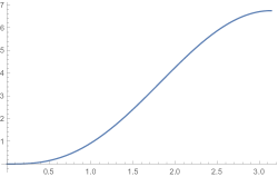
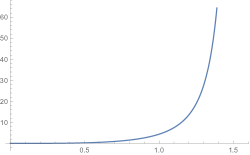
Figure 1: The curve $z(\theta)$ when $n=3,r=1$ (left), and $n=3,r=2$ (right)

We next give the proof of two key properties of the curve defined by (3).

Lemma 5.

Let $n,r\in\mathbb{N}$ be such that $\max\{n,r\}>1$, let ${\displaystyle{\phi=\frac{(n-1)\pi+r\theta}{n}}}$, and let $I$ be the interval as in Theorem 1. The function ${\displaystyle{z(\theta)=\frac{\sin^{n}\theta}{\sin^{n-r}(\phi-\theta)\sin^{r}(\phi)}}}$ is increasing on $(0,\pi/r)$, and maps this interval onto $I$.

Proof.

We start by computing three derivatives:

$$\frac{d}{d\theta}\left(\frac{\sin\theta}{\sin(\phi-\theta)}\right) = \frac{\cos\theta\sin(\phi-\theta)-\sin\theta\cos(\phi-\theta)\left(r/n-1\right)}{\sin^{2}(\phi-\theta)}$$ (7)

$$= \frac{\sin\phi-r\sin\theta\cos(\phi-\theta)/n}{\sin^{2}(\phi-\theta)},$$

$$\frac{d}{d\theta}\left(\frac{\sin\theta}{\sin\phi}\right)=\frac{\cos\theta\sin\phi-r\sin\theta\cos\phi/n}{\sin^{2}\phi},$$ (8)

and

$$\frac{d}{d\theta}\left(\frac{\sin(\phi-\theta)}{\sin\phi}\right) = \frac{\sin\phi\cos(\phi-\theta)(r/n-1)-r\sin(\phi-\theta)\cos\phi/n}{\sin^{2}\phi}$$ (9)

$$= \frac{r\sin\theta/n-\sin\phi\cos(\phi-\theta)}{\sin^{2}\phi}.$$

Armed with these calculations we now consider three cases, depending on the relative sizes of $n$ and $r$.

• In this case $z(\theta)$ simplifies to $z(\theta)=\sin\theta/\sin\phi$. This is an increasing function on $(0,\pi/r)$, since its derivative (8) is equal to ${\displaystyle{\frac{\sin((n-1)\pi/n)}{\sin((n-1)\pi/n+\theta)}}}$, a quantity strictly bigger than 0 for $\theta\in(0,\pi/r)$. Finally, we observe that $z(\theta)$ is continuous on $(0,\pi/r)$, ${\displaystyle{\lim_{\theta\to 0}z(\theta)=0}}$, and that ${\displaystyle{\lim_{\theta\to\pi/r}z(\theta)=+\infty}}$. We conclude that $z(\theta)$ maps $(0,\pi/r)$ to $(0,\infty)$.

• We write

  $$z(\theta)=\left(\frac{\sin\theta}{\sin(\phi-\theta)}\right)^{n-r}\left(\frac{\sin\theta}{\sin\phi}\right)^{r},$$

  and note that the inequalities

  $$\pi-\frac{\pi}{n}<\phi<\pi$$ (10)

  and

  $$\pi-\frac{\pi}{r}<\phi-\theta<\pi-\frac{\pi}{n}$$ (11)

  hold for $\theta\in(0,\pi/r)$. We now demonstrate that $\sin\theta/\sin(\phi-\theta)$ and $\sin\theta/\sin\phi$ are both increasing functions of $\theta$ on $(0,\pi/r)$. If $2\leq r<n$, then $\cos\theta>0$ and $\cos(\phi-\theta)<0$. Consequently (7) and (8) are positive. By checking the limits as $\theta\rightarrow 0$ and $\theta\rightarrow\pi/r$, we see that $z(\theta)$ maps $(0,\pi/r)$ onto $(0,\infty)$. If $r=1$ and $\theta\leq\pi/2$, then $\cos\theta\geq 0$ and $\cos(\phi-\theta)\leq 0$ and $z(\theta)$ is an increasing function of $\theta$ for the same reason.
  Finally, we treat the case when $r=1$ and $\pi>\theta>\pi/2$. We write

  $$\sin\phi=\sin\frac{(n-1)\pi+\theta}{n}=\sin\frac{\pi-\theta}{n},$$

  and note that for any angle $0<\alpha<\pi/2$, the inequality

  $$\sin\frac{\alpha}{n}>\frac{1}{n}\sin\alpha$$

  holds, as the two sides agree when $\alpha=0$ and the derivative of the left side is greater than that of the right side when $0<\alpha<\pi/2$. Thus $\sin\phi>\sin\theta/n$ and (7) is positive. To show (8) is positive, we note that for any angle $0<\alpha<\pi/2$, the inequality

  $$\frac{1}{n}\sin\alpha\cos\frac{\alpha}{n}>\cos\alpha\sin\frac{\alpha}{n}$$ (12)

  holds since the two sides are equal when $\alpha=0$ and their respective derivatives satisfy

  $$\frac{1}{n}\cos\alpha\cos\frac{\alpha}{n}-\frac{1}{n^{2}}\sin\alpha\sin\frac{\alpha}{n}>\frac{1}{n}\cos\alpha\cos\frac{\alpha}{n}-\sin\alpha\sin\frac{\alpha}{n}.$$

  Applying (12) with $\alpha=\pi-\theta$ establishes that (8) is positive. Thus $z(\theta)$ is an increasing function for all pairs $r,n$ under consideration. We next compute

  $$\lim_{\theta\rightarrow\pi}\frac{\sin\theta}{\sin(\phi-\theta)} = \lim_{\theta\rightarrow\pi}\frac{\sin(\pi-\theta)}{\sin\left((n-1)(\pi-\theta)/n\right)}=\frac{n}{n-1},$$ (13)

  $$\lim_{\theta\rightarrow\pi}\frac{\sin\theta}{\sin\phi} = \lim_{\theta\rightarrow\pi}\frac{\sin(\pi-\theta)}{\sin((\pi-\theta)/n)}=n.$$ (14)

  Consequently, if $1=r<n$, then $z(\theta)$ maps the interval $(0,\pi)$ to $(0,n^{n}/(n-1)^{n-1})$.

• We apply arguments akin to those above to the function

  $$z(\theta)=\left(\frac{\sin\theta}{\sin\phi}\right)^{n}\left(\frac{\sin(\phi-\theta)}{\sin\phi}\right)^{r-n}$$

  and see that $z(\theta)$ is an increasing function of $\theta$ on $(0,\pi/r)$. If $n>1$, then $z$ maps $(0,\pi/r)$ onto $(0,\infty$). If $n=1$, we compute

  $$\lim_{\theta\rightarrow 0}\frac{\sin\theta}{\sin\phi} = \frac{1}{r}\qquad\text{and}$$ (15)

  $$\lim_{\theta\rightarrow 0}\frac{\sin(\phi-\theta)}{\sin\phi} = \frac{r-1}{r},$$ (16)

  and conclude that $z(\theta)$ maps the interval $(0,\pi/r)$ onto $((r-1)^{r-1}/r^{r},\infty)$. The proof is complete.

∎

We now reformulate the condition $D_{n,r}(t,z)=0$ by rescaling the zeros of $D_{n,r}(t,z)$. Although it may seem insignificant at first, this change in point of view will enable to us derive key magnitude estimates for these zeros (see Proposition 6). These estimates in turn lay the foundation for the asymptotic analysis, and with that for the proof of Theorem 1, in Section 3.
We proceed as follows. Suppose $t=|t|e^{-i\theta}$ is a zero of $D_{n,r}(t,z)$, set

$$t_{0} = \frac{\sin\phi}{\sin(\phi-\theta)}e^{-i\theta}\qquad\text{(see (\ref{eq:t0form})), and}$$

$$t_{1} = t_{0}e^{2i\theta}=\overline{t_{0}}.$$

After labeling the remaining $\max\{n,r\}-2$ zeros of $D_{n,r}(t,z)$ as $t_{2},t_{3},\ldots,t_{\max\{n,r\}-1}$, write

$$q_{k} = \frac{t_{k}}{t_{0}},\qquad\text{and}$$

$$\zeta_{k} = q_{k}e^{-i\theta}\qquad\text{for}\quad 0\leq k<\max\{n,r\}.$$

With this notation we rewrite $(1-t_{k})^{n}+zt_{k}^{r}=0$ as

$$-z=\frac{(1-t_{k})^{n}}{t_{k}^{r}}=\frac{(t_{0}^{-1}-q_{k})^{n}}{q_{k}^{r}}t_{0}^{n-r}.$$

Combining (5) with (3) we see that $D_{n,r}(t_{k},z)=0$ if and only if

$$-\frac{\sin^{n}\theta}{\sin^{n-r}(\phi-\theta)\sin^{r}\phi}=\frac{\left(\sin(\phi-\theta)/\sin\phi-\zeta_{k}\right)^{n}}{\zeta_{k}^{r}}\left(\frac{\sin\phi}{\sin(\phi-\theta)}\right)^{n-r},$$

or equivalently

$$\left(\frac{\sin(\phi-\theta)}{\sin\phi}-\zeta_{k}\right)^{n}+\zeta_{k}^{r}\left(\frac{\sin\theta}{\sin\phi}\right)^{n}=0.$$ (17)

We remark that $k=0,1$ correspond to the two trivial solutions of (17), namely $\zeta_{0}=e^{-i\theta}$ and $\zeta_{1}=e^{i\theta}$. The next proposition establishes that these are the solutions of (17) of smallest magnitude.

Proposition 6.

Suppose $n,r\in\mathbb{N}$ are such that $\max\{n,r\}>1$, $\theta\in(0,\pi/r)$ and $\phi=((n-1)\pi+r\theta)/n$. The polynomial

$$Q(\zeta)=\left(\frac{\sin(\phi-\theta)}{\sin\theta}-\zeta\frac{\sin\phi}{\sin\theta}\right)^{n}+\zeta^{r}$$ (18)

has exactly two zeros on the unit circle. All other zeros of $Q(\zeta)$ lie outside the closed unit disk $|\zeta|\leq 1$.

Proof.

We replace $\zeta$ by $\zeta^{n}$ and consider the zeros of

$$\widetilde{Q(\zeta)}=\left(\frac{\sin(\phi-\theta)}{\sin\theta}-\zeta^{n}\frac{\sin\phi}{\sin\theta}\right)^{n}+\zeta^{rn}.$$

Note that if $\zeta$ is a zero of $\widetilde{Q(\zeta)}$, then $\zeta$ is a zero of

$$R(\zeta) = \sin(\phi-\theta)-\zeta^{n}\sin\phi-\omega\zeta^{r}\sin\theta$$

$$= \sin\theta(-\omega\zeta^{r}-\cos\phi)-\sin\phi(\zeta^{n}-\cos\theta),$$

where $\omega=\exp\{i(\pi+2\pi k)/n\}$ for some $0\leq k<n$. Consequently, it suffices to establish the result for $R(\zeta)$.
Zeros of $R(\zeta)$ on the unit circle. Consider the image of the unit circle $\zeta=e^{i\psi}$, $0\leq\psi<2\pi$, under $R$:

$$R(e^{i\psi})=\sin\theta(e^{i(r\psi+\alpha)}-\cos\phi)-\sin\phi(e^{in\psi}-\cos\theta),\qquad 0\leq\psi<2\pi,$$

where

$$\alpha=\pi+\frac{\pi+2k\pi}{n},\qquad\text{for some}\quad 0\leq k<n.$$

The two curves

$$C_{1} : \qquad\sin\theta(e^{i(r\psi+\alpha)}-\cos\phi),\qquad 0\leq\psi<2\pi\quad\text{and}$$

$$C_{2} : \qquad\sin\phi(e^{in\psi}-\cos\theta)\qquad 0\leq\psi<2\pi$$

are circles with radii $r_{1}=\sin\theta,r_{2}=\sin\phi$ and centers $z_{1}=-\sin\theta\cos\phi,z_{2}=-\sin\phi\cos\theta$ respectively. (see Figure 3 when $\cos\theta>0$ and $\cos\phi<0$). Thus, the equality $R(e^{i\psi})=0$ holds only when these two circles intersect, and hence the solutions of $R(\zeta)=0$ on the unit circle must satisfy $n\psi\equiv\pm\theta\mbox{ (mod $2\pi$)}$, or equivalently, $\zeta^{n}=e^{\pm i\theta}$.

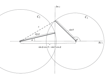
Figure 2: Generic positioning of the two circles $C_{1}$ and $C_{2}$

A priori we don’t know where the points of intersection (if any) of the two circles $C_{1}$ and $C_{2}$ are. A quick calculation using the law of cosines shows however, that in Figure 2, we must in fact have $x=\sin\phi$, and we obtain the more accurate Figure 3.

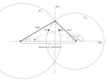
Figure 3: The two circles $C_{1}$ and $C_{2}$

Zeros of $R(\zeta)$ inside the unit disk. We claim that the loop $\Gamma:=R(e^{i\psi})$, $0\leq\psi<2\pi$, does not intersect the ray $(-\infty,0)$, and hence the winding number of $\Gamma$ about any point on $(-\infty,0)$ is $0$. We demonstrate the claim by treating three different cases, distinguished by whether $r$, $n$, or neither is equal to one.
If $r\geq 2$ and $n\geq 2$, then $\cos\theta>0$ and $\cos\phi<0$. Suppose, by way of contradiction, that $\Gamma$ intersects the ray $(-\infty,0)$. Then modulo $2\pi$ the inequalities

$$-\theta<n\psi<\theta\quad\text{and}$$

$$\phi<r\psi+\alpha<2\pi-\phi$$

must hold. Whence, the points $p_{1}$ and $p_{2}$ (on $C_{1}$ and $C_{2}$ respectively) corresponding to $\psi$ must lie on the arc of $C_{1}(C_{2}$ resp) that is inside of $C_{2}(C_{1}$ resp), (see Figure 3). Write

$$\theta-n\psi \equiv \beta\pmod{2\pi}\quad\text{and}$$ (20)

$$r\psi+\alpha-\phi \equiv \gamma\pmod{2\pi}$$ (21)

where, given the symmetry about the $x$-axis, we may without loss of generality assume that $0<\beta\leq\theta$ and $0<\gamma\leq(\pi-r\theta)/n$. We add $r$ times the first congruence to $n$ times the second congruence and obtain

$$r\beta+n\gamma\equiv 0\mbox{ (mod $2\pi$)},$$

which is impossible since $0<r\beta+n\gamma\leq\pi$.
If $n=1$, the fact that the zeros of the function

$$R(\zeta)=\sin((r-1)\theta)-\zeta\sin r\theta+\zeta^{r}\sin\theta$$

lie outside the open unit disk is a direct consequence of Lemma 8 in [9]. If $r=1$, we write $R(\zeta)$ as

$$R(\zeta) = \sin\theta(-\omega\zeta-\cos\phi)-\sin\phi(\zeta^{n}-\cos\theta)$$

$$= \sin(\pi-\theta)\left(-\omega\zeta+\cos\frac{\pi-\theta}{n}\right)-\sin\frac{\pi-\theta}{n}\left(\zeta^{n}+\cos(\pi-\theta)\right).$$

Applying the substitutions $\omega\zeta\rightarrow\zeta$, $(\pi-\theta)/n\rightarrow\theta$, and $n\rightarrow r$, reduces this case to the case $n=1$, and completes the proof. ∎

We close this section with a result concerning the multiplicities of the zeros of $Q(\zeta)$, in addition to their location furbished by Proposition 6.

Lemma 7.

Let $n,r\in\mathbb{N}$ be such that $\max\{n,r\}>1$, $0<\theta<\pi/r$, and ${\displaystyle{\phi=\frac{(n-1)\pi+r\theta}{n}}}$. The zeros of the polynomial

$$Q(\zeta)=\left(\frac{\sin(\phi-\theta)}{\sin\theta}-\zeta\frac{\sin\phi}{\sin\theta}\right)^{n}+\zeta^{r}$$

are distinct, except when

1. $n>r>1$ and $r$ is odd, or

2. $r>n>1$ and $n$ is odd .

If (1) or (2) hold, then there exists a unique $\theta^{*}\in(0,\pi/r)$ so that $Q(\zeta)$ has one double zero, and all of its remaining zeros are distinct.

Proof.

Suppose that $\zeta_{*}$ is a multiple zero of $Q(\zeta)$, that is, $Q(\zeta_{*})=Q^{\prime}(\zeta_{*})=0$. If $n=r$, $\zeta_{*}$ would have to satisfy $\zeta_{*}^{n-1}(\sin(\phi-\theta)/\sin\phi)=0$, and hence $\zeta_{*}=0$. Since $Q(0)\neq 0$, we conclude that if $n=r$, $Q(\zeta)$ has no multiple zeros.
If $n\neq r$, the equations $Q(\zeta_{*})=0=Q^{\prime}(\zeta_{*})$ imply that

$$Q^{\prime}(\zeta_{*}) = -n\frac{\sin\phi}{\sin\theta}\left(\frac{\sin(\phi-\theta)}{\sin\theta}-\zeta_{*}\frac{\sin\phi}{\sin\theta}\right)^{n-1}+r\zeta_{*}^{r-1}$$

$$= \zeta_{*}^{r-1}\left(n\frac{\zeta_{*}\sin\phi}{\sin(\phi-\theta)-\zeta_{*}\sin\phi}+r\right)$$

$$= 0.$$

We note that (2) has the unique non-zero solution

$$\zeta_{*}=-\frac{r}{n-r}\frac{\sin(\phi-\theta)}{\sin\phi}.$$

Substituting this expression into the equation $Q(\zeta^{*})=0$ yields

$$\frac{\sin^{n}(\phi-\theta)}{\sin^{n}\theta}\left(\frac{n^{n}}{(n-r)^{n}}+(-1)^{r}\frac{r^{r}}{(n-r)^{r}}\frac{\sin^{n}\theta}{\sin^{r}\phi\sin^{n-r}(\phi-\theta)}\right)=0.$$ (23)

By Lemma 5, the left hand side of equation (23) does not vanish for $\theta\in(0,\pi/r)$, unless (1) or (2) hold, in which case it vanishes for a unique value $\theta^{*}\in(0,\pi/r)$. ∎

3 The proof of Theorem 1

We now turn our attention to the proof of Theorem 1, which admittedly is technical. As such, that the reader may benefit from seeing the proof of a special case before proceeding to the general case. Recall that the generating function $1/D_{n,r}(t,z)$ of the sequence $\left\{P_{m}(z)\right\}_{m=0}^{\infty}$ depends on $n,r\in\mathbb{N}$. If $\max\{n,r\}=2$, the result in Theorem 1 is in fact a consequence of Theorem 1 in [8]. In the following proposition we treat the case $\max\{n,r\}=3$. As it turns out, in this case the conclusions of Theorem 1 can be strengthened to $P_{m}(z)$ having only real zeros for all $m\geq 0$.

Proposition 8.

Suppose that $n,r\in\mathbb{N}$ be such that $\max\{n,r\}=3$. Let $D_{n,r}(t,z)=(1-t)^{n}+zt^{r}$, and let $I$ be the real interval in the statement of Theorem 1. Suppose further that

$$\sum_{m=0}^{\infty}P_{m}(z)t^{m}=\frac{1}{D_{n,r}(t,z)},$$

and write $\mathcal{Z}(P_{m})$ for the set of zeros of $P_{m}(z)$. Then $\mathcal{Z}(P_{m})\subset I$ for all $m\geq 0$, and ${\displaystyle{\bigcup_{m=0}^{\infty}\mathcal{Z}(P_{m})}}$ is dense in $I$.

Proof.

Suppose $\theta\in(0,\pi/r)$ and let $z\in I$ be the point so that $t_{0}=|t_{0}|e^{-i\theta},\,t_{1}=t_{0}e^{2i\theta}$ and $t_{2}\in\mathbb{R}$ are the zeros of $D_{n,r}(t,z)$. Note that by Lemma 7, $t_{0},t_{1}$ and $t_{2}$ are distinct. Thus by partial fraction decomposition we obtain

$$\frac{1}{D_{n,r}(t,z)} = -\frac{1}{(t-t_{0})(t_{0}-t_{1})(t_{0}-t_{2})}-\frac{1}{(t-t_{1})(t_{1}-t_{0})(t_{1}-t_{2})}-\frac{1}{(t-t_{2})(t_{2}-t_{0})(t_{2}-t_{1})}$$

$$= \sum_{m=0}^{\infty}\left(\frac{1}{(t_{0}-t_{1})(t_{0}-t_{2})}\frac{1}{t_{0}^{m+1}}+\frac{1}{(t_{1}-t_{0})(t_{1}-t_{2})}\frac{1}{t_{1}^{m+1}}+\frac{1}{(t_{2}-t_{0})(t_{2}-t_{1})}\frac{1}{t_{2}^{m+1}}\right)t^{m},$$

and consequently, for all $m\geq 0$,

$$P_{m}(z)=\frac{1}{t_{0}^{m+1}(t_{0}-t_{1})(t_{0}-t_{2})}+\frac{1}{t_{1}^{m+1}(t_{1}-t_{0})(t_{1}-t_{2})}+\frac{1}{t_{2}^{m+1}(t_{2}-t_{0})(t_{2}-t_{1})}.$$ (24)

We set $q_{1}=t_{1}/t_{0}$, $q_{2}=t_{2}/t_{0}$, and divide the right hand side of (24) by $t_{0}^{m+3}$ to conclude that $z$ is a zero of $P_{m}(z)$ if and only if

$$\frac{1}{(1-q_{1})(1-q_{2})}+\frac{1}{q_{1}^{m+1}(q_{1}-1)(q_{1}-q_{2})}+\frac{1}{q_{2}^{m+1}(q_{2}-1)(q_{2}-q_{1})}=0.$$ (25)

By multiplying the left hand side of (25) by $e^{(m+3)i\theta}$ we obtain the equivalent equation

$$-\frac{1}{2i\sin\theta e^{-i(m+1)\theta}(e^{-i\theta}-\zeta_{2})}+\frac{1}{2i\sin\theta e^{i(m+1)\theta}(e^{i\theta}-\zeta_{2})}+\frac{1}{\zeta_{2}^{m+1}(\zeta_{2}^{2}-2\cos\theta\zeta_{2}+1)}=0,$$

where $\zeta_{2}:=q_{2}e^{-i\theta}\in\mathbb{R}$ since $t_{2}\in\mathbb{R}$. Combining the first two summands and factoring the expression ${\displaystyle{\frac{1}{\zeta_{2}^{2}-2\zeta_{2}\cos\theta+1}}}$ establishes that equation (25) is equivalent to

$$\frac{\sin(m+2)\theta-\zeta_{2}\sin(m+1)\theta}{\sin\theta}+\frac{1}{\zeta_{2}^{m+1}}=0.$$ (26)

Finally, using the identity $\sin(m+2)\theta=\sin(m+1)\theta\cos\theta+\cos(m+1)\theta\sin\theta$, we see that equation (26) holds if and only if $\theta$ is a zero of

$$R_{m}(\theta)=\frac{(\cos\theta-\zeta_{2})\sin(m+1)\theta}{\sin\theta}+\cos(m+1)\theta+\frac{1}{\zeta_{2}^{m+1}}.$$ (27)

According to Proposition 6, $|\zeta_{2}|>1$, and hence the sign of $R_{m}(\theta)$ alternates at values of $\theta$ for which $\cos(m+1)\theta=\pm 1$. Thus, by the Intermediate Value Theorem, there are at least $\left\lfloor m/r\right\rfloor$ zeros $\theta$ of $R_{m}(\theta)$ on $(0,\pi/r)$. Lemma 5 in turn implies that each of these zeros $\theta$ yields an distinct zero $z(\theta)$ of $P_{m}(z)$ on $I$. Since the degree of $P_{m}(z)$ is $\left\lfloor m/r\right\rfloor$, we see that $\mathcal{Z}(P_{m})\subset I$ for all $m\geq 0$. Finally, note that the set of solutions to $\cos(m+1)\theta=\pm 1$, $m\geq 0$, is dense in $(0,\pi/r)$, which immediately implies that ${\displaystyle{\bigcup_{m=0}^{\infty}\mathcal{Z}(P_{m})}}$ is dense in $I$, and completes the proof. ∎

We continue with some remarks regarding Theorem 1 in the case when $\max\{n,r\}>3$ and $m$ is large. If the the zeros $t_{k}$, $0\leq k<\max\{n,r\}$, of $D_{n,r}(t,z)$ are distinct, then the partial fraction decomposition of ${\displaystyle{\frac{1}{D_{n,r}(t,z)}}}$ gives

$$\sum_{m=0}^{\infty}P_{m}(z)t^{m} = \pm\prod_{k=1}^{\max(n,r)-1}\frac{1}{t-t_{k}}$$

$$= \pm\sum_{k=0}^{\max(n,r)-1}\frac{1}{t-t_{k}}\prod_{l\neq k}\frac{1}{t_{k}-t_{l}}$$

$$= \pm\sum_{m=0}^{\infty}\left(\sum_{k=0}^{\max(n,r)-1}\frac{1}{t_{k}^{m+1}}\prod_{l\neq k}\frac{1}{t_{k}-t_{l}}\right)t^{m}.$$

Equating coefficients of powers of $t$ in these formal power series shows that for any $m\geq 0$, the equation $P_{m}(z)=0$ is equivalent to

$$\sum_{k=0}^{\max(n,r)-1}\frac{1}{t_{k}^{m+1}}\prod_{l\neq k}\frac{1}{t_{k}-t_{l}}=0.$$ (28)

We multiply equation (28) by $t_{0}^{m+\max\{n,r\}}$ and by $e^{(m+\max\{n,r\})i\theta}$ and conclude that $z$ is a zero of $P_{m}(z)$ if and only if $\theta$ is a zero of

$$R_{m}(\theta) := \sum_{k=0}^{\max(n,r)-1}\frac{1}{\zeta_{k}^{m+1}}\prod_{l\neq k}\frac{1}{\zeta_{k}-\zeta_{l}}$$ (29)

$$= \sum_{k=0}^{\max\{n,r\}-1}\frac{1}{\zeta_{k}^{m+1}Q^{\prime}(\zeta_{k})},$$

where $\zeta_{k}=e^{-i\theta}t_{k}/t_{0}$, $0\leq k<\max\{n,r\}-1$, are the roots of

$$Q(\zeta)=\left(\frac{\sin(\phi-\theta)}{\sin\theta}-\zeta\frac{\sin\phi}{\sin\theta}\right)^{n}+\zeta^{r}$$

with $\phi=((n-1)\pi+r\theta)/n$. Using symmetric reduction we conclude that $R_{m}(\theta)$ is a real valued continuous function of $\theta$ on $(0,\pi/r)$.
If $D_{n,r}(t,z)$ has zeros of multiplicity greater than one, then so does $Q(\zeta)$. Thus we must be in either case (1) or (2) in Lemma 7, and hence there exists a unique $\theta^{*}\in(0,\pi/r)$ corresponding to the double zero $\zeta_{*}$ of $Q(\zeta)$. It is clear that $R_{m}(\theta)$ has a singularity at $\theta^{*}$. We claim that this singularity is removable. Indeed, if $\zeta_{a}=\zeta_{b}=\zeta_{*}$ for some $0\leq a<b<\max\{n,r\}-1$, then the sum of the two terms of $R_{m}(\theta)$ involving both $\zeta_{a}$ and $\zeta_{b}$ is equal to

$$\frac{m+1}{\zeta_{a}^{m+2}}\prod_{l\neq a,b}\frac{1}{\zeta_{a}-\zeta_{l}}.$$

Thus we may consider $R(\theta)$ to be a real valued continuous function of $\theta$ on $(0,\pi/r)$, regardless of whether or not the zeros of $D_{n,r}(t,z)$ are distinct.
Recall that the magnitude estimates of Proposition 6 allowed us to dispense with the term in $R_{m}(\theta)$ corresponding to the third zero of $Q(\zeta)$ in Proposition 8. In order to make a similar approach work in the general case, we will need the following calculations concerning the dominating terms in $R_{m}(\theta)$.
Assume that $\theta\in(0,\pi/r)$, set ${\displaystyle{\phi=\frac{(n-1)\pi+r\theta}{n}}}$, and recall that $\zeta_{0,1}=e^{\mp i\theta}$ are the two trivial zeros of $Q(\zeta)$ of minimal magnitude. Using the identity

$$\sin(\phi-\theta)-e^{i\theta}\sin\phi=-\sin\theta e^{i\phi},$$

we rewrite the expression for $Q^{\prime}(\zeta)$ in (2) as

$$Q^{\prime}(e^{i\theta}) = e^{(r-1)i\theta}\left(-n\frac{\sin\phi}{\sin\theta}e^{i(\theta-\phi)}+r\right).$$

Thus sum of the two terms in (29) corresponding $\zeta_{0}=e^{-i\theta}$ and $\zeta_{1}=e^{i\theta}$ can be written as

$$2\frac{\Re\left(e^{i(m+1)\theta}Q^{\prime}(e^{i\theta})\right)}{|Q^{\prime}(e^{i\theta})|^{2}}=\frac{2}{|Q^{\prime}(e^{i\theta})|^{2}}\left(A\cos(m+r)\theta-B\sin(m+r)\theta\right),$$ (30)

where

$$A=A(\theta) = -n\frac{\sin\phi}{\sin\theta}\cos(\phi-\theta)+r,$$ (31)

$$B=B(\theta) = n\frac{\sin\phi}{\sin\theta}\sin(\phi-\theta).$$

Just as we did in the proof of Proposition 8, we will demonstrate that the sign of $R_{m}(\theta)$ changes at points where $\cos(m+r)\theta=\pm 1$. At such points $B(\theta)=0$, so in order to be able to track the exact number of sign changes in $R_{m}(\theta)$, it remains to describe the function $A(\theta)$, which we do in the next lemma.

Lemma 9.

Let $n,r\in\mathbb{N}$ be such that $\max\{n,r\}>1$, suppose that $\theta\in(0,\pi/r)$ and set $\phi=((n-1)\pi+r\theta)/n$. The function

$$A(\theta)=-n\frac{\sin\phi}{\sin\theta}\cos(\phi-\theta)+r$$

is strictly positive.

Proof.

If $\cos(\phi-\theta)\leq 0$ then $A(\theta)>0$ since $\sin\phi>0$ and $\sin\theta>0$ on the interval under consideration. Consequently, if $r\geq 2$ and $n\geq 2$, then $A(\theta)>0$.
If $r=1$, then $A(\theta)>0$ if and only if

$$\sin\theta-n\sin\phi\cos(\phi-\theta)>0.$$

Note that the left side of the above inequality is $0$ when $\theta=\pi$, and it is a decreasing function of $\theta$ on $(0,\pi)$ because its derivative is negative there:

$$\frac{d}{d\theta}\left(\sin\theta-n\sin\phi\cos(\phi-\theta)\right)$$

$$= \cos\theta-\cos\phi\cos(\phi-\theta)+n\sin\phi\sin(\phi-\theta)\left(\frac{1}{n}-1\right)$$

$$= (2-n)\sin\phi\sin(\phi-\theta)$$

$$< 0.$$

It follows that if $r=1$, then $A(\theta)>0$.
Finally, if $n=1$, then $\phi=r\theta$, and

$$A(\theta)\sin\theta = r\sin\theta-\sin\phi\cos(\phi-\theta)$$

$$= (r-1)\sin\theta-\cos\phi\sin(\phi-\theta).$$

Since $A(0)\sin(0)=0$, and

$$\frac{d}{d\theta}(A(\theta)\sin(\theta))=(2r-1)\sin(r\theta)\sin((r-1)\theta)>0$$

for $\theta\in(0,\pi/r)$, we conclude that $A(\theta)>0$ in this case as well. ∎

We are now in position to describe the sign changes of $R_{m}(\theta)$ on the interval $(0,\pi/r)$.

Proposition 10.

Suppose that $n,r\in\mathbb{N}$ are such that $\max\{n,r\}>1$, and let $R_{m}(\theta)$ be defined as in equation (29) for $m\geq 0$. If ${\displaystyle{\theta_{h}=\frac{h\pi}{m+r},(h=1,\ldots,\left\lfloor m/r\right\rfloor),}}$ denote the values of $\theta$ in $(0,\pi/r)$ which give $\cos(m+r)\theta=\pm 1$, then

• $\textrm{sgn}\left(R_{m}(\theta_{h})\right)=(-1)^{h}$, and

• $\textrm{sgn}\left(R_{m}(\pi/r^{-})\right)=(-1)^{\left\lfloor m/r\right\rfloor+1}$.

for all $m$ sufficiently large.

Proof.

The proof is broken into three cases as dictated by the asymptotic behavior of the expressions $\theta_{h}$ as $m$ goes to infinity. Some of these will stay bounded away from both zero and $\pi/r$, some will approach $0$, and some will tend to $\pi/r$.

Case 1: $\gamma<\theta<\pi/r-\gamma$ for some small fixed $\gamma$ independent of $m$

Proposition 6 implies that if $2\leq k<\max(n,r)$, then $|\zeta_{k}|>1+\epsilon$ for some fixed $\epsilon>0$. Using Lemma 9 and equation (30) we write

$$R_{m}(\theta)=\frac{2}{|Q^{\prime}(e^{i\theta})|^{2}}\left(A\cos(m+r)\theta-B\sin(m+r)\theta\right)+\sum_{k=2}^{\max(n,r)-1}\frac{1}{\zeta_{k}^{m+1}Q^{\prime}(\zeta_{k})},$$

where the $A(\theta)>0$ and the sum approaches $0$ exponentially fast when $m\rightarrow\infty$. We invoke Lemma 9 to conclude that the sign of $R_{m}(\theta_{h})$ is $(-1)^{h}$.

Case 2: $\theta\rightarrow 0$ as $m\rightarrow\infty$

If $n=1$, the zeros $e^{\pm i\theta}$ of $Q(\zeta)$ converge to $1$, while its remaining zeros converge to those zeros of $T(\zeta)=r-1-r\zeta+\zeta^{r}$ which are greater than one in magnitude, and hence are uniformly separated from the closed unit disk. Thus, following an argument similar to the one in Case 1, we see that the sum in

$$R_{m}(\theta)=\frac{2}{|Q^{\prime}(e^{i\theta})|^{2}}\left(A\cos(m+r)\theta-B\sin(m+r)\theta\right)+\sum_{k=2}^{\max(n,r)-1}\frac{1}{\zeta_{k}^{m+1}Q^{\prime}(\zeta_{k})},$$

approaches $0$ exponentially fast as $m\rightarrow\infty$. We next calculate

$$A(\theta) = r-\frac{\sin(r\theta)\cos((r-1)\theta)}{\sin\theta}$$

$$= \left(\frac{r}{3}-r^{2}+\frac{2r^{3}}{3}\right)\theta^{2}+\mathcal{O}(\theta^{4}),$$

and deduce that $A(\theta)\to 0$ at a polynomial rate. Consequently, the sign of $R_{m}(\theta_{h})$ is $(-1)^{h}$ for $m\gg 1$.

On the other hand, if $n\neq 1$, then $Q(\zeta)$ has $n$ zeros in a neighborhood of $1$, and the possible remaining $\max\{n,r\}-n$ zeros lie outside the closed unit disk. Assume without loss of generality that $\zeta_{k}$ is in a neighborhood of $1$ for $0\leq k<n$. For the same reason as in Case 1, the sum

$$\sum_{k=n}^{\max(r,n)-1}\frac{1}{\zeta_{k}^{m+1}Q^{\prime}(\zeta_{k})}$$

is either $0$, or it approaches $0$ exponentially fast. We next consider the sum

$$\sum_{k=0}^{n-1}\frac{1}{\zeta_{k}^{m+1}Q^{\prime}(\zeta_{k})}.$$

Set $\zeta=1+\epsilon$, $\epsilon\in\mathbb{C}$, and note that

$$\sin\left(\phi-\theta\right)-\zeta\sin\phi = \sin\frac{\pi+(n-r)\theta}{n}-\zeta\sin\frac{\pi-r\theta}{n}$$ (32)

$$= \sin\frac{\pi}{n}+\left(\cos\frac{\pi}{n}\right)\left(\frac{(n-r)\theta}{n}\right)-(1+\epsilon)\sin\frac{\pi}{n}+(1+\epsilon)\left(\cos\frac{\pi}{n}\right)\left(\frac{r\theta}{n}\right)+\mathcal{O}\left(\theta^{2}\right)$$

$$= \theta\cos\frac{\pi}{n}+\frac{r\theta\epsilon}{n}\cos\frac{\pi}{n}-\epsilon\sin\frac{\pi}{n}+\mathcal{O}\left(\theta^{2}\right).$$

Thus, if $\zeta$ is a zero of $Q(\zeta)$, then

$$0=\left(\theta\cos\frac{\pi}{n}+\frac{r\theta\epsilon}{n}\cos\frac{\pi}{n}-\epsilon\sin\frac{\pi}{n}+\mathcal{O}(\theta^{2})\right)^{n}+\theta^{n}(1+\epsilon)^{r}(1+\mathcal{O}(\theta)).$$

We deduce that

$$\theta\cos\frac{\pi}{n}+\frac{r\theta\epsilon}{n}\cos\frac{\pi}{n}-\epsilon\sin\frac{\pi}{n}=\omega\theta\left(1+\epsilon\right)^{r/n}\left(1+\mathcal{O}\left(\theta\right)\right),$$

where $\omega$ is an $n$-th root of $-1$. Expanding $(1+\epsilon)^{n/r}$ and solving for $\epsilon$ yields

$$\epsilon=\frac{\theta\left(\cos(\pi/n)-\omega\right)}{\sin(\pi/n)}+\mathcal{O}\left(\theta^{2}\right).$$ (33)

Substituting (32) and (33) into the expression (2) for $Q^{\prime}(\zeta)$ we see that if $\zeta$ is a zero of $Q(\zeta)$, then

$$Q^{\prime}(\zeta) = \zeta^{r-1}\left(n\frac{\zeta\sin\phi}{\sin(\phi-\theta)-\zeta\sin\phi}+r\right)$$ (34)

$$= \zeta^{r-1}\left(\frac{n\zeta\sin(\pi/n)}{\theta\omega}+\mathcal{O}(1)\right).$$

Thus,

$$\sum_{k=0}^{n-1}\frac{1}{\zeta_{k}^{m+1}Q^{\prime}(\zeta_{k})}=\frac{\theta}{n\sin(\pi/n)}\sum_{k=0}^{n-1}\frac{\omega_{k}}{\zeta_{k}^{m+r}}\left(1+\mathcal{O}(\theta)\right),$$ (35)

where $\omega_{k}=e^{(2k-1)\pi i/n}$, $0\leq k<n$.

If $\theta\geq\delta/\sqrt{m}$ for some small $\delta$, then equation (33) gives

$$|\zeta_{k}| \geq \left|1+\frac{\theta(\cos(\pi/n)-\omega_{k})}{\sin(\pi/n)}\right|$$

$$> \left|1+\frac{\delta\left(\cos(\pi/n)-\cos\left((2k-1)\pi/n\right)\right)}{2\sqrt{m}\sin(\pi/n)}\right|.$$

From this inequality we deduce that when $m$ is large,

$$\sum_{k=2}^{n-1}\frac{1}{\zeta_{k}^{m+1}Q^{\prime}(\zeta_{k})}$$

approaches $0$ faster than the polynomial decay of $\frac{2}{|Q^{\prime}(e^{i\theta})|^{2}}\left(A\cos(m+r)\theta-B\sin(m+r)\theta\right)$. Thus the sign of $R_{m}(\theta_{h})$ is again $(-1)^{h}$ for $m\gg 1$.
On the other hand, if $\theta<\delta/\sqrt{m}$ for $\delta\ll 1$, then

$$\zeta_{k}^{m+r} = \left(1+\frac{\theta(\cos(\pi/n)-\omega_{k})}{\sin(\pi/n)}+\mathcal{O}(\theta^{2})\right)^{m+r}$$

$$= \exp\left(\frac{\cos(\pi/n)-\omega_{k}}{\sin(\pi/n)}h\pi\right)\left(1+\mathcal{O}\left(\frac{h^{2}}{m}\right)\right).$$

We select $\delta$ small enough so that the sign of $R_{m}(\theta_{h})$ is the same as the sign of

$$\sum_{k=0}^{n-1}\omega_{k}\exp^{-1}\left(\frac{\cos(\pi/n)-\omega_{k}}{\sin(\pi/n)}h\pi\right),$$

which in turn is determined by the sign of

$$\sum_{k=0}^{n-1}\omega_{k}\exp\left(\frac{h\pi\omega_{k}}{\sin(\pi/n)}\right),$$

since ${\displaystyle{\exp^{-1}\left(\cos(\pi/n)/\sin(\pi/n)\right)>0}}$. The next lemma establishes that the sign of the expression in question is $(-1)^{h}$, thereby completing Case 2.

Lemma 11.

Suppose that $n\geq 2$. Then for al $h\in\mathbb{N}$, the sign of the expression

$$\sum_{k=0}^{n-1}\omega_{k}\exp^{-1}\left(\frac{\cos(\pi/n)-\omega_{k}}{\sin(\pi/n)}h\pi\right),$$ (36)

is $(-1)^{h}$.

Proof.

Note that the sum of the first two terms of (36) is

$$2(-1)^{h}\cos\left(\frac{\pi}{n}\right),$$

whereas the sum of the remaining $n-2$ terms is at most

$$\sum_{k=2}^{n-1}\exp^{-1}\left(\frac{\cos(\pi/n)-\cos((2k-1)\pi/n)}{\sin(\pi/n)}h\pi\right),$$ (37)

a sum which is largest when $h=1$. We use a computer to check that when $n\leq 85$ and $h=1$, (37) is less than $|2\cos(\pi/n)|$, hence the sign of (36) is $(-1)^{h}$. For $n>85$ we bound (37) as follows:

$$\sum_{k=2}^{n-1}\exp^{-1}\left(\frac{\cos(\pi/n)-\cos((2k-1)\pi/n)}{\sin(\pi/n)}h\pi\right) = \sum_{k=2}^{n-1}\exp^{-1}\left(2\frac{h\pi}{\sin(\pi/n)}\sin\frac{k\pi}{n}\sin\frac{(k-1)\pi}{n}\right)$$

$$< 2\sum_{k=2}^{\left\lfloor n/2\right\rfloor}\exp^{-1}\left(2h\pi\sin\frac{k\pi}{n}\right)$$

$$\stackrel{{\scriptstyle(i)}}{{<}} 2\sum_{k=2}^{\left\lfloor n/2\right\rfloor}\exp^{-1}\left(\frac{hk\pi^{2}}{n}\right)$$

$$\stackrel{{\scriptstyle(ii)}}{{<}} \frac{2}{e^{h\pi^{2}/n}(e^{h\pi^{2}/n}-1)},$$

where inequality $(i)$ follows from the fact that $2\sin(k\pi/n)>k\pi/n$ when $k<n/2$, and inequality $(ii)$ is obtained by replacing the partial geometric sum by the whole series. The reader will note that the inequality

$$\frac{2}{e^{h\pi^{2}/n}(e^{h\pi^{2}/n}-1)}<2\cos\frac{\pi}{85}<2\cos\frac{\pi}{n}$$

holds when $e^{h\pi^{2}/n}>1.62$, or when $n<20h$. Consequently, when $n<20h$,

$$\sum_{k=2}^{n-1}\omega_{k}\exp^{-1}\left(\frac{\cos(\pi/n)-\omega_{k}}{\sin(\pi/n)}h\pi\right)<|2\cos(\pi/n)|$$

and the sign of (36) is $(-1)^{h}$.
Consider now the case $h<n/20$. We note that $n>85$ implies that

$$\sum_{k=0}^{n-1}\omega_{k}\exp\left(\frac{h\pi\omega_{k}}{\sin(\pi/n)}\right)\approx\sum_{k=0}^{n-1}\omega_{k}e^{hn\omega_{k}}.$$

By expanding the exponential function in a series we obtain

$$\sum_{k=0}^{n-1}\omega_{k}e^{hn\omega_{k}} = \sum_{k=0}^{n-1}\omega_{k}\sum_{j=0}^{\infty}\frac{1}{j!}\left(hn\omega_{k}\right)^{j}$$ (38)

$$= \sum_{j=0}^{\infty}\frac{1}{j!}(hn)^{j}\left(\sum_{k=0}^{n-1}\omega_{k}^{j+1}\right).$$

The identity

$$\sum_{k=0}^{n-1}\omega_{k}^{a}=\left\{\begin{array}[]{cc}0&\text{if}n\nmid a\\ n(-1)^{a/n}&\text{if }n\mid a\end{array}\right.,$$

simplifies (38) to

$$n\sum_{j=1}^{\infty}(-1)^{j}\frac{1}{(nj-1)!}\left(hn\right)^{jn-1}=:n\sum_{j=1}^{\infty}a_{j}.$$

It is straightforward to show that $|a_{j}|<|a_{j+1}|$ for $j=0,1,\ldots,h-1$, and $|a_{j}|>|a_{j+1}|$ for $j=h,h+1,\ldots$. Since the sum $\sum a_{j}$ is alternating, we conclude that

$$\left|\sum_{j=0}^{h-1}a_{j}\right|<|a_{h-1}|,\qquad\text{and}\qquad\left|\sum_{j=h+1}^{\infty}a_{j}\right|<|a_{h+1}|.$$

We now relate the quantities $|a_{h-1}|,|a_{h}|$ and $|a_{h+1}|$. To this end, we compute

$$\left|\frac{a_{j+1}}{a_{j}}\right|=\frac{(hn)^{n}}{\prod_{\ell=0}^{n-1}nj+\ell},$$

and consequently,

$$\frac{|a_{h-1}|+|a_{h+1}|}{|a_{h}|} = \frac{\prod_{\ell=0}^{n-1}(n(h-1)+\ell)}{(nh)^{n}}+\frac{(hn)^{n}}{\prod_{\ell=0}^{n-1}(nh+\ell)}$$

$$= \prod_{\ell=0}^{n-1}\left(1-\frac{n-\ell}{n}\frac{1}{h}\right)+\frac{1}{\prod_{\ell=1}^{n-1}\left(1+\frac{\ell}{nh}\right)}$$

$$= P_{1}+\frac{1}{P_{2}}.$$

Taking the natural logarithm of $P_{1}$ we obtain

$$\ln(P_{1}) = \sum_{\ell=0}^{n-1}\ln\left(1-\frac{n-\ell}{n}\frac{1}{h}\right)$$

$$\stackrel{{\scriptstyle\ast}}{{<}} \sum_{\ell=0}^{n-1}\left(-\frac{n-\ell}{n}\frac{1}{h}\right)$$

$$= -\frac{1}{nh}\frac{n(n+1)}{2}$$

$$= -\frac{n+1}{2h},$$

where the starred inequality follows from the fact that $\ln x\leq x-1$ for all $x>0$, with equality only when $x=1$. We conclude that $P_{1}<\exp(-\frac{n+1}{2h})$. On the other hand, taking the natural logarithm of $P_{2}$ gives

$$\ln(P_{2}) = \sum_{\ell=1}^{n-1}\ln\left(1+\frac{\ell}{nh}\right)$$

$$\stackrel{{\scriptstyle\ast}}{{>}} \sum_{\ell=1}^{n-1}\frac{\ell}{2nh}$$

$$= \frac{1}{2nh}\frac{(n-1)n}{2}$$

$$= \frac{n-1}{4h},$$

where for the starred inequality we used the fact that $\ln x>\frac{x-1}{2}$ for $1<x<2$. Consequently, ${\displaystyle{P_{2}>\exp\left(\frac{n-1}{4h}\right)}}$. Combining these two results we see that

$$P_{1}+\frac{1}{P_{2}}<e^{-\frac{n+1}{2h}}+e^{-\frac{n-1}{4h}}<1,$$

which in turn implies that $|a_{h-1}|+|a_{h+1}|<|a_{h}|$, and hence

$$\left|\sum_{j\neq h}a_{j}\right|<|a_{h}|$$

when $h<n/20$ and $n>85$. Thus, the sign of the expression (36) is $(-1)^{h}$ in this case as well. ∎

Case 3: $\theta\rightarrow\pi/r$ as $m\rightarrow\infty$

When $\theta\rightarrow\pi/r$ and $r=1$, we observe that with $R(\zeta)$ as in (2), the polynomial

$$\frac{R(\zeta)}{\sin\theta}=(-\omega\zeta-\cos\phi)-\frac{\sin\phi}{\sin\theta}(\zeta^{n}-\cos\theta)$$

converges locally uniformly to

$$\widetilde{T}(\zeta)=(1-\omega\zeta)-\frac{1}{n}(1+\zeta^{n}).$$

A quick calculation shows that

$$n\widetilde{T}(\zeta)\big{|}_{\omega\zeta\to\zeta}=T(\zeta),$$ (39)

the polynomial we treated at the beginning of case 2. Since the transformations used in (39) preserve the location of the zeros in, on, and outside the unit circle, we conclude that as $\theta\rightarrow\pi/r$, $Q(\zeta)$ converges locally uniformly to a polynomial whose zeros lie outside the closed unit disk besides the double zeros at $\zeta=-1$. As a result, the sign of $R_{m}(\theta_{h})$ is again determined by the sign of $\cos(m+r)\theta_{h}$, and is hence equal to $(-1)^{h}$.
When $r>1$, the polynomial $Q(\zeta)$ has $r$ zeros approaching the $r$-th roots of $-1$, with the possible remaining $n-r$ zeros (when $n>r)$ tending to $\infty$. We thus consider the sum

$$\sum_{k=0}^{r-1}\frac{1}{\zeta_{k}^{m+1}Q^{\prime}(\zeta_{k})}$$

where each $\zeta_{k}$, $0\leq k<r$, approaches an $r$-th root of $-1$. We set $e_{k}=e^{(2k-1)\pi i/r}$ and $\zeta_{k}=e_{k}+\epsilon$, for some $\epsilon\in\mathbb{C}$, and write

$$\eta=\frac{\pi}{r}-\theta=\frac{\pi}{r}-\frac{h\pi}{m+r}=\frac{m+r-hr}{r(m+r)}\pi.$$

We compute the difference

$$\sin\left(\phi-\theta\right)-\zeta\sin\phi = \sin\frac{\pi+(n-r)\theta}{n}-\zeta\sin\frac{\pi-r\theta}{n}$$

$$= \sin\frac{\pi}{r}+\frac{(r-n)\eta}{n}\cos\frac{\pi}{r}-\zeta\frac{r\eta}{n}+\mathcal{O}(\eta^{2}),$$

and use it to rewrite the equation $Q(\zeta_{k})=0$ as

$$0 = \left(\sin\frac{\pi}{r}+\frac{(r-n)\eta}{n}\cos\frac{\pi}{r}-(e_{k}+\epsilon)\frac{r\eta}{n}\right)^{n}+(\sin\frac{\pi}{r}-\eta\cos\frac{\pi}{r})^{n}(e_{k}+\epsilon)^{r}+\mathcal{O}(\eta^{2})$$

$$= \left(\sin\frac{\pi}{r}+\frac{(r-n)\eta}{n}\cos\frac{\pi}{r}-e_{k}\frac{r\eta}{n}\right)^{n}-(\sin\frac{\pi}{r}-\eta\cos\frac{\pi}{r})^{n}\left(1+\frac{r\epsilon}{e_{k}}\right)+\mathcal{O}(\eta^{2}+\epsilon^{2}).$$

Taking $n$-th roots yields

$$\frac{(r-n)\eta}{n}\cos\frac{\pi}{r}-e_{k}\frac{r\eta}{n}=\frac{r\epsilon}{ne_{k}}\sin\frac{\pi}{r}-\eta\cos\frac{\pi}{r}\left(1+\frac{r\epsilon}{ne_{k}}\right)+\mathcal{O}(\eta^{2}+\epsilon^{2}),$$

and consequently

$$\epsilon=\frac{e_{k}(\cos(\pi/r)-e_{k})\eta}{\sin(\pi/r)-\eta\cos(\pi/r)}+\mathcal{O}\left(\eta^{2}\right)=\frac{e_{k}(\cos(\pi/r)-e_{k})\eta}{\sin(\pi/r)}+\mathcal{O}(\eta^{2}).$$ (40)

From equation (2) we also obtain

$$Q^{\prime}(\zeta_{k}) = \zeta_{k}^{r-1}\left(n\frac{\zeta_{k}\sin\phi}{\sin(\phi-\theta)-\zeta\sin\phi}+r\right)$$

$$= r\zeta_{k}^{r-1}+\mathcal{O}(\eta)$$

which we substitute into the sum under consideration to obtain

$$\sum_{k=0}^{r-1}\frac{1}{\zeta_{k}^{m+1}Q^{\prime}(\zeta_{k})}=\frac{1}{r}\sum_{k=0}^{r-1}\frac{1+\mathcal{O}(\eta)}{\zeta_{k}^{m+r}}.$$ (41)

For the same reasons as in Case 2, it suffices to consider $\eta<\delta/\sqrt{m}$ for small $\delta$. In this case we have the approximation

$$\zeta_{k}^{m+r} = e_{k}^{m+r}\left(1+\frac{\cos(\pi/r)-e_{k}}{\sin(\pi/r)}\eta+\mathcal{O}(\eta^{2})\right)^{m+r}$$

$$= e_{k}^{m+r}\exp\left(\frac{\cos(\pi/r)-e_{k}}{\sin(\pi/r)}(m+r)\eta\right)\left(1+\mathcal{O}\left(m\eta^{2}\right)\right).$$

We choose $\delta$ small so that the sign of $R_{m}(\theta_{h})$ is the same as the sign of

$$\sum_{k=0}^{r-1}e_{k}^{-m-r}\exp^{-1}\left(\frac{\cos(\pi/r)-e_{k}}{\sin(\pi/r)}\left(\frac{m}{r}-h+1\right)\pi\right).$$ (42)

The sum of the first two terms in the above sum is $2(-1)^{h}$ and hence, for reasons similar to those in Case 2 (i.e. using the same argument with $m/r-h+1$ in place of $h$), it suffices to consider $r>85$. For such $r$, arguments entirely analogous to those we gave in the proof of Lemma 11 establish that the sign of the sum (42) is $(-1)^{h}$. The determine the sign of $R(\pi/r^{-})$, we first note that for $r>85$, the sign of (42) is the same as that of

$$\sum_{k=0}^{r-1}e_{k}^{-m-r}e^{(m-rh+r)e_{k}}=\sum_{k=0}^{r-1}e_{k}^{-m-r}\sum_{j=0}^{\infty}\frac{1}{j!}\left((m-rh+r)e_{k}\right)^{j}.$$ (43)

If we let $m=pr+s$, $0\leq s<r$, then the double summation on the right hand side of (43) can be rewritten as

$$r\sum_{j=0}^{\infty}(-1)^{p+1-j}\frac{\left(m+r-rh\right)^{jr+s}}{(rj+s)!}.$$ (44)

Now the sign of $R(\pi/r^{-})$ is obtained by replacing $h$ by $(m+r)/r^{-}$ in (42), and thus by setting $j=0$ in (44). By doing so we conclude that the sign of $R(\pi/r^{-})$ is $(-1)^{p+1}=(-1)^{\lfloor\frac{m}{r}\rfloor+1}$. The proof is complete. ∎ With Proposition 10 at our disposal, we now put the finishing touches on the proof of Theorem 1. Let $n,r\in\mathbb{N}$ such that $\max\{r,n\}>1$, and suppose that

$$\sum_{m=0}^{\infty}P_{m}(z)t^{m}=\frac{1}{(1-t)^{n}+zt^{r}}=:\frac{1}{D_{n,r}(t,z)}.$$

Given $m\in\mathbb{N}$, every zero of $R_{m}(\theta)$ (see (29)) corresponds to a distinct zero $z\in I$ of $P_{m}(z)$. Proposition 10, together with the Intermediate Value Theorem imply that for $m\gg 1$, $R_{m}(\theta)$ has at least $\left\lfloor m/r\right\rfloor$ zeros on $(0,\pi/r)$. The conclusions of Theorem 1 now follow from degree considerations, along with the density of the solutions of the equations $\cos(m+r)\theta=\pm 1$, $m=0,1,\ldots$, in the interval $(0,\pi/r)$.

4 Some open problems

In light of the conclusions of Theorem 1 and Proposition 8, it is natural to ask whether the zeros of $P_{m}(z)$ lie on $I$ for all $m$.

Problem 12.

Let $n,r\in\mathbb{N}$ such that $\max\{n,r\}>1$. We consider the sequence of polynomials $P_{m}(z)$ generated by

$$\sum_{m=0}^{\infty}P_{m}(z)t^{m}=\frac{1}{(1-t)^{n}+zt^{r}},$$

and write $\mathcal{Z}(P_{m})$ for the set of zeros of $P_{m}(z)$. Show that $\mathcal{Z}(P_{m})\subset I$ for all $m\geq 0$, and ${\displaystyle\bigcup_{m=0}^{\infty}\mathcal{Z}(P_{m})}$ is dense in $I$ where

$$I=\left\{\begin{array}[]{cc}(0,\infty)&\text{if}n,r\geq 2\\ (0,n^{n}/(n-1)^{n-1})&\text{if }r=1\\ ((r-1)^{r-1}/r^{r},\infty)&\text{ if }n=1\end{array}\right..$$

A natural way to extend the problem is to consider, in place of the binomial expression $(1-t)^{n}$, any polynomial with real positive zeros (such polynomials also play a key role in the theory of multiplier sequences). We formalize this extension in

Problem 13.

Let $Q(t)\in\mathbb{R}[t]$ be a real polynomial in $t$ whose zeros are positive real numbers and $Q(0)>0$. Show that for any integer $r\geq 0$, the zeros of the polynomial $P_{m}(z)$ generated by

$$\sum_{m=0}^{\infty}P_{m}(z)t^{m}=\frac{1}{Q(t)+zt^{r}}$$

lie on the positive real ray.

As we have seen in the proof of Lemma 3, the denominator of the generating function gives the recurrence relation for $P_{m}(z)$ whereas the numerator gives rise to the set of initial polynomials. Allowing for more general numerators in the rational generating function is a natural extension of the current work. With some numerical evidence in support, we propose the following

Problem 14.

Let $Q(t)\in\mathbb{R}[t]$ be a real polynomial in $t$ whose zeros are positive real numbers and $Q(0)>0$. For any integer $r\geq 0$ and any real bivariate polynomial $N(t,z)\in\mathbb{R}[t,z]$ whose degree in $t$ is less than the degree in $t$ of $Q(t)+zt^{r}$, we consider the sequence of polynomials $P_{m}(z)$ generated by

$$\sum_{m=0}^{\infty}P_{m}(z)t^{m}=\frac{N(t,z)}{Q(t)+zt^{r}}.$$

Show that there is a fixed constant (depending perhaps on $r$ and $\deg Q$) $C$ such that for any $m$, the number of zeros of $P_{m}(z)$ outside $(0,\infty)$ is less than $C$.

Finally, although in this paper we do not study them explicitly, transformations $T$ with the property that the sequence of polynomials $\left\{P_{m}^{T}(z)\right\}_{m=0}^{\infty}$ generated by $T[G(t,z)]$ have only real zeros whenever those generated by $G(t,z)$ do are of great interest. We see a natural parallel between these operators, and reality preserving linear operators on $\mathbb{R}[x]$, and believe that understanding them is key to understanding how polynomial sequences with only real zeros might be generated. As such, we pose

Problem 15.

Classify operators (bi-linear, or otherwise) $T$ on $\mathbb{R}(t,z)$ with the property that all terms of the sequence of polynomials $\left\{P_{m}^{T}(z)\right\}_{m=0}^{\infty}$ generated by $T[G(t,z)]$ have only real zeros whenever those generated by $G(t,z)$ do. Any results regarding this problem would be pioneering, even if $G(t,z)$ is restricted to be a rational function of the type discussed in the present paper.

References

- [1] S. Beraha, J. Kahane, N. J. Weiss, Limits of zeros of recursively defined polynomials, Proc. Nat. Acad. Sci. U.S.A., 72 (1975), no. 11, 4209.
- [2] J. Borcea and P. Brändén, Pólya-Schur master theorems for circular domains and their boundaries, Annals of Math., 170 (2009), 465-492.
- [3] T. Forgács and A. Piotrowski, Hermite multiplier sequences and their associated operators, Constr. Approx. 43(3) (2015), pp. 459-479. DOI 10.1007/s00365-015-9277-3
- [4] G. H. Hardy, On the zeros of certain class of integral Taylor series II, Proc. London Math. Soc. (2) 2 (1905), 401-431.
- [5] I. V. Ostrovskii, Hardy’s generalization of and related analogs of cosine and sine, Comput. Methods Funct. Theory 6 (2006), no. 1, 1-14.
- [6] J. Peetre. Une caractérisation abstraite des opérateurs différentiels. In: Mathematica Scandinavica 7.0 (1959). Issn:1903-1807.
- [7] G. Pólya and J. Schur, Über zwei Arten von Faktorenfolgen in der Theorie der algebraischen Gleichungen, J. Reine Angew. Math., 144 (1914), 89-113.
- [8] K. Tran, Connections between discriminants and the root distribution of polynomials with rational generating function, J. Math. Anal. Appl. 410 (2014), 330–340.
- [9] K. Tran, The root distribution of polynomials with a three-term recurrence, J. Math. Anal. Appl. 421 (2015), 878–892.
- [10] A. Sokal, Chromatic roots are dense in the whole complex plane, Combin. Probab. Comput., 13 (2004), 221-261.