TMD Evolution at Moderate Hard Scales

Abstract:

We summarize some of our recent work on non-perturbative transverse momentum dependent (TMD) evolution, emphasizing aspects that are necessary for dealing with moderately low scale processes like semi-inclusive deep inelastic scattering.
PoS.cls, January 11, 2016, JLAB-THY-16-2196, DOE/OR/23177-3644

1 TMD factorization and non-perturbative evolution

The purpose of this talk is to summarize results recently presented in Ref. [1]. We will discuss the Collins-Soper-Sterman (CSS) form of TMD factorization in the updated version presented in Ref. [2]. (See Ref. [3] for a general overview and for references.) For these proceedings, the relevant aspects of the TMD factorization theorems are the following:

• The unpolarized cross section for a process like Drell-Yan scattering is expressible as

  $$\frac{\mathop{\mathrm{d}\mskip-0.59999mu\sigma}\nolimits}{\mathop{\mathrm{d}^{4}\mskip-0.59999muq}\nolimits\mathop{\mathrm{d}\mskip-0.59999mu\Omega}\nolimits}$$

  $${}\;=\frac{2}{s}\sum_{j}{\color{red}\frac{\mathop{\mathrm{d}\mskip-0.59999mu\hat{\sigma}_{j\bar{\jmath}}}\nolimits(Q,\mu\to Q;\alpha_{s}(Q))}{\mathop{\mathrm{d}\mskip-0.59999mu\Omega}\nolimits}}\int\mathop{\mathrm{d}^{2}\mskip-0.59999mu{\bf b}}\nolimits~{}e^{i{\bf q}_{\text{T}}\cdot{\bf b}}~{}{\color{blue}\tilde{F}_{j/A}(x_{A},{\bf b};Q^{2},Q)}~{}$$

  $${}\;+\text{large $q_{\text{T}}$ ``Y-term'' correction}\,.$$ (1)

  where ${\color{red}\mathop{\mathrm{d}\mskip-0.59999mu\hat{\sigma}_{j\bar{\jmath}}}\nolimits/\mathop{\mathrm{d}\mskip-0.59999mu\Omega}\nolimits}$ is a hard partonic cross section and ${\color{blue}\tilde{F}(x,{\bf b};Q^{2},Q)}$ is a TMD parton distribution function (PDFs) in coordinate space evaluated with a hard scale $Q$.

• Collins-Soper (CS) evolution applied to an individual TMD PDF leads to

  $$\frac{\partial}{\partial\ln Q}{\ln\color{blue}\tilde{F}_{j/A}(x_{A},{\bf b}_{\text{T}};Q^{2},Q)}={\tilde{K}(b_{\text{T}};Q)}+\;b_{\text{T}}\,\,\text{Independent Terms}$$ (2)

  The “$b_{\text{T}}\,\,\text{Independent Terms}$” only affect the normalization of $\tilde{F}$ but not its shape.

• The kernel $\tilde{K}(b_{\text{T}};Q)$ is is strongly universal. At small $b_{\text{T}}$ its $b_{\text{T}}$-dependence is perturbatively calculable with $1/b_{\text{T}}$ acting as a hard scale. At large $b_{\text{T}}$ its $b_{\text{T}}$-dependence is non-perturbative.

• For all $b_{\text{T}}$, $\tilde{K}(b_{\text{T}};Q)$ obeys the renormalization group (RG) equation:

  $$\frac{\mathop{\mathrm{d}\mskip-0.59999mu}\nolimits}{\mathop{\mathrm{d}\mskip-0.59999mu\ln\mu}\nolimits}\tilde{K}(b_{\text{T}};\mu)=-\gamma_{K}\left(\alpha_{s}(\mu)\right)\,.$$ (3)

  At small $b_{\text{T}}$, one hopes to exploit perturbation theory with $1/b_{\text{T}}$ as a hard scale to calculate $\tilde{K}(b_{\text{T}};Q)$ while at large $b_{\text{T}}$ a non-perturbative parametrization is needed. In the non-perturbative region, one hopes to exploit the strong universality of $\tilde{K}(b_{\text{T}};Q)$ to make predictions. One needs a prescription to demarcate what constitutes large and small $b_{\text{T}}$. To smoothly interpolate between the two regions, one imposes a gentle cutoff on large $b_{\text{T}}$. A common choice of cutoff function is

  $${\bf b}_{*}({\bf b}_{\text{T}})=\frac{{\bf b}_{\text{T}}}{\sqrt{1+b_{\text{T}}^{2}/b_{\rm max}^{2}}}\,.$$ (4)

  Then an RG scale defined as $\mu_{b_{*}}\equiv C_{1}/b_{*}$ approaches $C_{1}/b_{\text{T}}$ at small $b_{\text{T}}$ and $C_{1}/b_{\rm max}$ at large $b_{\text{T}}$. We can separate $\tilde{K}(b_{\text{T}};Q)$ into a large $b_{\text{T}}$ part and a small $b_{\text{T}}$ part by adding and subtracting $\tilde{K}(b_{*};Q)$ in Eq. (2):

  $$\frac{\partial}{\partial\ln Q}{\ln\color{blue}\tilde{F}_{j/A}(x_{A},{\bf b}_{\text{T}};Q^{2},Q)}=\tilde{K}(b_{*};Q)+\left[\tilde{K}(b_{\text{T}};Q)-\tilde{K}(b_{*};Q)\right]+\;b_{\text{T}}\,\,\text{Independent Terms}\,.$$ (5)

  The $g_{K}(b_{\text{T}};b_{\rm max})$ function is defined as the term $\tilde{K}(b_{\text{T}};Q)-\tilde{K}(b_{*};Q)$, so that

  $$\frac{\partial}{\partial\ln Q}{\ln\color{blue}\tilde{F}_{j/A}(x_{A},{\bf b}_{\text{T}};Q^{2},Q)}=\tilde{K}(b_{*};Q)-g_{K}(b_{\text{T}};b_{\rm max})+\;b_{\text{T}}\,\,\text{Independent Terms}\,.$$ (6)

  By definition, the right side of Eq. (6) is exactly independent of $b_{\rm max}$. From Eq. (3), $g_{K}(b_{\text{T}};b_{\rm max})$ is also exactly independent of $Q$. The $Q$ dependence in each of the terms in the definition of $g_{K}(b_{\text{T}};b_{\rm max})$ cancels. We can apply Eq. (3) to exploit RG improvement in the calculation of $\tilde{K}(b_{*};Q)$:

  $$\tilde{K}(b_{*};Q)=\tilde{K}(b_{*};\mu_{b_{*}})-\int_{\mu_{b_{*}}}^{Q}\frac{\mathop{\mathrm{d}\mskip-0.59999mu\mu^{\prime}}\nolimits{}}{\mu^{\prime}}\gamma_{K}(\alpha_{s}(\mu^{\prime})).$$ (7)

  So, the evolution of the shape of $\tilde{F}_{j/A}(x_{A},{\bf b}_{\text{T}};Q^{2},Q)$ is is given by

  $$\frac{\partial}{\partial\ln Q}{\ln\color{blue}\tilde{F}_{j/A}(x_{A},{\bf b}_{\text{T}};Q^{2},Q)}$$

  $$\;{}={\color{red}\tilde{K}(b_{*};\mu_{b_{*}})-\int_{\mu_{b_{*}}}^{Q}\frac{\mathop{\mathrm{d}\mskip-0.59999mu\mu^{\prime}}\nolimits{}}{\mu^{\prime}}\gamma_{K}(\alpha_{s}(\mu^{\prime}))}-{\color{blue}g_{K}(b_{\text{T}};b_{\rm max})}+\;b_{\text{T}}\,\,\text{Independent Terms}\,.$$ (8)

  The partial derivative symbol means $x_{A}$ is to be held fixed. The $g_{K}(b_{\text{T}};b_{\rm max})$ function inherits the universality properties of $\tilde{K}(b_{\text{T}};\mu)$. In particular, it is related to the vacuum expectation value of a relatively simple Wilson loop. It is independent of any details of the process and is even the same if the PDF $\tilde{F}_{j/A}(x_{A},{\bf b}_{\text{T}};Q^{2},Q)$ is replaced with a fragmentation function. Thus we say that $g_{K}(b_{\text{T}};b_{\rm max})$ is “strongly” universal; see the graphic in Fig. 1.

  

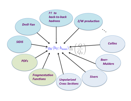
  Figure 1: Strong universality of the non-perturbative evolution parametrized by $g_{K}(b_{\text{T}};b_{\rm max})$. The $-g_{K}(b_{\text{T}};b_{\rm max})\ln(Q/Q_{0})$ combination appears exponentiated in the evolved cross section expression.

  The $g_{K}(b_{\text{T}};b_{\rm max})$ function is often called the “non-perturbative” part of the evolution since it can contain non-perturbative elements. This is a slight misnomer, however, since $g_{K}(b_{\text{T}};b_{\rm max})$ can contain perturbative contributions as well. Indeed, at very small $b_{\text{T}}$ it is entirely perturbatively calculable, though suppressed by powers of $b_{\text{T}}/b_{\rm max}$, according to its definition in Eq. (5).

  2 Large $b_{\text{T}}$ behavior

  A common choice for non-perturbative parametrizations of $g_{K}(b_{\text{T}};b_{\rm max})$ is a power-law form. These tend to yield reasonable success in fits that involve at least moderately high scales $Q$ [4]. However, extrapolations of those fits to lower values of $Q$ (such as those corresponding to many current SIDIS experiments) appear to appear to produce evolution that is far too rapid [5, 6]. In this talk, we carefully examine the underlying physics issues surrounding non-perturbative evolution and, on the basis of those considerations, we will propose a form for $g_{K}(b_{\text{T}};b_{\rm max})$ that accommodates both large and small $Q$ behavior.

  We will first write down our proposed ansatz for $g_{K}(b_{\text{T}};b_{\rm max})$ and then spend the remainder of the talk discussing its justifications. Our proposal is

  $${\color{blue}g_{K}(b_{\text{T}};b_{\rm max})}\\ =g_{0}(b_{\rm max})\left(1-\exp\left[-\frac{C_{F}\alpha_{s}(\mu_{b_{*}})b_{\text{T}}^{2}}{\pi g_{0}(b_{\rm max})\,b_{\rm max}^{2}}\right]\right)\,,$$ (9)

  where

  $$g_{0}(b_{\rm max})=g_{0}({b_{\rm max}}_{,0})+\frac{2C_{F}}{\pi}\int_{C_{1}/{b_{\rm max}}_{,0}}^{C_{1}/b_{\rm max}}\frac{\mathop{\mathrm{d}\mskip-0.59999mu\mu^{\prime}}\nolimits{}}{\mu^{\prime}}\alpha_{s}(\mu^{\prime})\,.$$ (10)

  The only parameter of the model is $g_{0}(b_{\rm max})$ and it varies with $b_{\rm max}$ according to Eq. (10). ${b_{\rm max}}_{,0}$ is a boundary value for $g_{0}$ relative to which other values are determined.

  First, note that the a small $b_{\text{T}}/b_{\rm max}$ expansion of Eq. (9) gives

  $${\color{blue}g_{K}(b_{\text{T}};b_{\rm max})}=\frac{C_{F}}{\pi}\frac{b_{\text{T}}^{2}}{b_{\rm max}^{2}}\alpha_{s}(\mu_{b_{*}})+O\left(\frac{b_{\text{T}}^{4}C_{F}^{2}\alpha_{s}(\mu_{b_{*}})^{2}}{b_{\rm max}^{4}\pi^{2}g_{0}(b_{\rm max})}\right)\,,$$ (11)

  while an expansion of the exact definition of $-g_{K}(b_{\text{T}};b_{\rm max})$ in Eq. (5) is

  $${\color{blue}g_{K}(b_{\text{T}};b_{\rm max})} {}=-\tilde{K}(b_{\text{T}};\mu_{b_{*}};\alpha_{s}(\mu_{b_{*}}))+\tilde{K}(b_{*};\mu_{b_{*}};\alpha_{s}(\mu_{b_{*}}))$$

  $${}=\frac{C_{F}}{\pi}\frac{b_{\text{T}}^{2}}{b_{\rm max}^{2}}\alpha_{s}(\mu_{b_{*}})+O\left(\frac{b_{\text{T}}^{4}}{\pi^{2}b_{\rm max}^{4}}\alpha_{s}(\mu_{b_{*}})^{2}\right)$$ (12)

  So, the exact definition and Eq. (9) match in the small $b_{\text{T}}$ limit.

  3 Conditions on $g_{K}(b_{\text{T}};b_{\rm max})$

  Our description of the large $b_{\text{T}}$ limit of correlation functions like $\tilde{F}(x_{A},{\bf b}_{\text{T}};Q^{2},Q)$ is motivated by the general observation that the analytic properties of correlation functions imply an exponential coordinate dependence, with a possible power-law fall-off, for the large $b_{\text{T}}$ limit. That is, neglecting perturbative contributions,

  $$\tilde{F}(x_{A},{\bf b}_{\text{T}};Q^{2},Q)\stackrel{{\scriptstyle b_{\text{T}}\to\infty}}{{\sim}}\frac{1}{{b_{\text{T}}}^{\alpha}}e^{-mb_{\text{T}}}\,,$$ (13)

  with $m$ and $\alpha$ independent of $Q$. See, for example, Ref. [7]. Therefore, from Eq. (2), $\tilde{K}(b_{\text{T}};Q)$ must approach a $b_{\text{T}}$-independent constant at large $b_{\text{T}}$.

  The set of requirements on $g_{K}(b_{\text{T}};b_{\rm max})$ is

  1. $\tilde{K}(b_{\text{T}};\mu_{b_{*}})\stackrel{{\scriptstyle b_{\text{T}}\to 0}}{{=}}\tilde{K}(b_{\text{T}};C_{1}/b_{\text{T}})$ is calculable entirely in perturbation theory with $C_{1}/b_{\text{T}}$ playing the role of a hard scale.

  2. $\tilde{K}(b_{\text{T}};Q)$ approaches a constant at $b_{\text{T}}/b_{\rm max}\to\infty$. The constant can be $Q$-dependent, but the $Q$-dependence can be calculated perturbatively for all $b_{\text{T}}$ from Eq. (3).

  3. Because of item 2, $g_{K}(b_{\text{T}};b_{\rm max})$ must approach a constant at large $b_{\text{T}}$, but the constant depends on $b_{\rm max}$.

  4. At small $b_{\text{T}}$, $g_{K}(b_{\text{T}};b_{\rm max})$ is a power series in $(b_{\text{T}}/b_{\rm max})^{2}$ with perturbatively calculable coefficients, as in Eqs. (11,12).

  5. By definition, the right side of Eq. (8) is independent of $b_{\rm max}$ and this should be preserved as much as possible in the functional form that parametrizes $g_{K}(b_{\text{T}};b_{\rm max})$. For small $b_{\text{T}}$, this means

     $$\mathop{\text{asy}}_{b_{\text{T}}\ll b_{\rm max}}\left.\frac{\mathop{\mathrm{d}\mskip-0.59999mu}\nolimits}{\mathop{\mathrm{d}\mskip-0.59999mub_{\rm max}}\nolimits}g_{K}(b_{\text{T}};b_{\rm max})\right|_{\text{parametrized}}=\mathop{\text{asy}}_{b_{\text{T}}\ll b_{\rm max}}\left.\frac{\mathop{\mathrm{d}\mskip-0.59999mu}\nolimits}{\mathop{\mathrm{d}\mskip-0.59999mub_{\rm max}}\nolimits}g_{K}(b_{\text{T}};b_{\rm max})\right|_{\text{truncated PT}}$$ (14)

     where “parametrized” refers to a specific model of $g_{K}(b_{\text{T}};b_{\rm max})$ while “truncated PT” refers to a truncated perturbative expansion. Eqs. (11,12) satisfy this requirement through order $\alpha_{s}(\mu_{b_{*}})$.

  6. At large $b_{\text{T}}$, $b_{\rm max}$-independence of the exact $\tilde{K}(b_{\text{T}},\mu)$ implies that, to a useful approximation,

     $$\frac{\mathop{\mathrm{d}\mskip-0.59999mu}\nolimits}{\mathop{\mathrm{d}\mskip-0.59999mu\ln b_{\rm max}}\nolimits}g_{K}(b_{\text{T}}=\infty;b_{\rm max})=\left[\frac{\mathop{\mathrm{d}\mskip-0.59999mu\tilde{K}(b_{\rm max};C_{1}/b_{\rm max})}\nolimits}{\mathop{\mathrm{d}\mskip-0.59999mu\ln b_{\rm max}}\nolimits}-\gamma_{K}(\alpha_{s}(C_{1}/b_{\rm max}))\right]_{\text{truncated PT}}\,,$$ (15)

     as obtained from Eq. (7) and the definition of $g_{K}$. Equation (10) ensures that Eq. (9) satisfies Eq. (8) so long as everything is calculated only to order $\alpha_{s}(\mu_{b_{*}})$. Enforcing both Eq. (14) and Eq. (15) simultaneously means $g_{K}(b_{\text{T}};b_{\rm max})$ will produce a $b_{\rm max}$ independent contribution to $\tilde{K}(b_{\text{T}};Q)$ for all $b_{\text{T}}$ except perhaps for an intermediate region at the border between perturbative and non-perturbative $b_{\text{T}}$-dependence. The residual $b_{\rm max}$ dependence there can be reduced by calculating higher orders and refining knowledge of non-perturbative behavior.

  For a much more detailed discussion of these considerations, see Sect. VII of Ref. [1]. Equation (9) is one of the simplest models that satisfies all 6 of these properties simultaneously.

  4 Conclusion

  In Sect. 3 we enumerated properties that a model of $g_{K}(b_{\text{T}};b_{\rm max})$ needs tp ensure basic consistency in a calculation $\tilde{K}(b_{\text{T}};Q)$. A simple parametrization was proposed in Sect. 2.

  Note that a quadratic $(b_{\text{T}}/b_{\rm max})^{2}$ dependence at small $b_{\text{T}}$ emerges naturally from (9), but with a perturbatively calculable coefficient. Furthermore, the dependence is not exactly quadratic because the coefficients contain logarithmic $b_{\text{T}}$ dependence through $\alpha_{s}(\mu_{b_{*}})$.

  In a process dominated by very large $b_{\text{T}}$, Sect. 3 and Eq. (9) predict an especially simple evolution for the low-$Q$ cross section. Namely, the cross section scales as $(Q/Q_{0})^{a}$ where $a$ is combination of $g_{K}(\infty,b_{\rm max})$ and perturbatively calculable quantities. (See Eq. (85,86) of Ref. [1].)

  Future phenomenological work should include efforts to constrain $g_{0}$. Because of its strongly universal nature, this offers a relatively simple way to test TMD factorization.

  Acknowledgments

  This work was supported by DOE contract No. DE-AC05-06OR23177, under which Jefferson Science Associates, LLC operates Jefferson Lab., and by DOE grant No. DE-SC0013699.

References

-
[1]
J. Collins and T. Rogers,
“Understanding the large-distance behavior of transverse-momentum-dependent parton densities and the Collins-Soper evolution kernel,”
Phys. Rev. D 91, no. 7, 074020 (2015)
doi:10.1103/PhysRevD.91.074020
[arXiv:1412.3820 [hep-ph]].
-
[2]
J. Collins,
“Foundations of perturbative QCD,”
(Cambridge monographs on particle physics, nuclear physics and cosmology. 32)
-
[3]
T. C. Rogers,
“An Overview of Transverse Momentum Dependent Factorization and Evolution,”
arXiv:1509.04766 [hep-ph].
-
[4]
A. V. Konychev and P. M. Nadolsky,
“Universality of the Collins-Soper-Sterman nonperturbative function in gauge boson production,”
Phys. Lett. B 633, 710 (2006)
doi:10.1016/j.physletb.2005.12.063
[hep-ph/0506225].
-
[5]
P. Sun and F. Yuan,
“Transverse momentum dependent evolution: Matching semi-inclusive deep inelastic scattering processes to Drell-Yan and W/Z boson production,”
Phys. Rev. D 88, no. 11, 114012 (2013)
doi:10.1103/PhysRevD.88.114012
[arXiv:1308.5003 [hep-ph]].
-
[6]
C. A. Aidala, B. Field, L. P. Gamberg and T. C. Rogers,
“Limits on transverse momentum dependent evolution from semi-inclusive deep inelastic scattering at moderate ,”
Phys. Rev. D 89, no. 9, 094002 (2014)
doi:10.1103/PhysRevD.89.094002
[arXiv:1401.2654 [hep-ph]].
-
[7]
P. Schweitzer, M. Strikman and C. Weiss,
“Intrinsic transverse momentum and parton correlations from dynamical chiral symmetry breaking,”
JHEP 1301, 163 (2013)
doi:10.1007/JHEP01(2013)163
[arXiv:1210.1267 [hep-ph]].