Bayesian subset simulation

Abstract

We consider the problem of estimating a probability of failure $\alpha$, defined as the volume of the excursion set of a function $f:\mathds{X}\subseteq\mathds{R}^{d}\to\mathds{R}$ above a given threshold, under a given probability measure on $\mathds{X}$. In this article, we combine the popular subset simulation algorithm (Au and Beck, Probab. Eng. Mech. 2001) and our sequential Bayesian approach for the estimation of a probability of failure (Bect, Ginsbourger, Li, Picheny and Vazquez, Stat. Comput. 2012). This makes it possible to estimate $\alpha$ when the number of evaluations of $f$ is very limited and $\alpha$ is very small. The resulting algorithm is called Bayesian subset simulation (BSS). A key idea, as in the subset simulation algorithm, is to estimate the probabilities of a sequence of excursion sets of $f$ above intermediate thresholds, using a sequential Monte Carlo (SMC) approach. A Gaussian process prior on $f$ is used to define the sequence of densities targeted by the SMC algorithm, and drive the selection of evaluation points of $f$ to estimate the intermediate probabilities. Adaptive procedures are proposed to determine the intermediate thresholds and the number of evaluations to be carried out at each stage of the algorithm. Numerical experiments illustrate that BSS achieves significant savings in the number of function evaluations with respect to other Monte Carlo approaches.

62L05, 62K99, 62P30

1 Introduction

Probabilistic reliability analysis has become over the last thirty years an essential part of the engineer’s toolbox (see, e.g., [44, 19, 47]). One of the central problems in probabilistic reliability analysis is the computation of the probability of failure

(1) $$\alpha\;=\;\int_{\mathds{X}}{\mathds{1}}_{f\leq 0}\,\mathrm{d}\mathsf{P}_{\mathds{X}}$$

of a system (or a component in a multicomponent system; see, e.g., [48], where $\mathsf{P}_{\mathds{X}}$ is a probability measure over some measurable space $\left(\mathds{X},\mathcal{B}\right)$ representing all possible sources of uncertainty acting on the system—both epistemic and aleatory—and $f:\mathds{X}\to\mathds{R}$ is the so-called limit-state function, such that $f$ takes positive values when the system behaves reliably, and negative values when the system behaves unreliably, or fails. It is assumed in this article that $\mathds{X}$ is a subset of $\mathds{R}^{d}$—in other words, we consider reliability problems where all uncertain factors can be described as a $d$-dimensional random vector. Numerous examples of applications that fall into this category can be found in the literature (see, for instance, [54, 39, 18, 5, 55, 34]).

Two major difficulties usually preclude a brute-force Monte Carlo (MC) approach, that is, using the estimator

$$\widehat{\alpha}^{\mskip 1.0mu\text{\tiny MC}}=\frac{1}{m}\sum_{i=1}^{m}{\mathds{1}}_{f(X_{i})\leq 0}\,,\quad X_{i}\stackrel{{\scriptstyle\rm i.i.d}}{{\sim}}\mathsf{P}_{\mathds{X}}\,,$$

which requires $m$ evaluations of $f$. First, the evaluation of $f$ for a given $x\in\mathds{X}$ often relies on one or several complex computer programs (e.g., partial differential equation solvers) that take a long time to run. Second, in many applications, the failure region $\Gamma=\{x\in\mathds{X}\mid f(x)\leq 0\}$ is a rare event under the probability $\mathsf{P}_{\mathds{X}}$; that is, the probability of failure $\alpha=\mathsf{P}_{\mathds{X}}(\Gamma)$ is small. When $\alpha$ is small, the standard deviation of $\widehat{\alpha}^{\mskip 1.0mu\text{\tiny MC}}$ is approximately $\sqrt{\alpha/m}$. To estimate $\alpha$ by MC with a standard deviation of $0.1\alpha$ thus requires approximately $100/\alpha$ evaluations of $f$. As an example, with $\alpha=10^{-3}$ and $10$ minutes per evaluation, this means almost two years of computation time.

The first issue—designing efficient algorithms to estimate $\alpha$ in the case of an expensive-to-evaluate limit-state function—can be seen as a problem of design and analysis of computer experiments (see, e.g., [50]), bearing some similarities to the problem of global optimization (see [53] and references therein). Several sequential design strategies based on Gaussian process models have been proposed in the literature, and spectacular evaluation savings have been demonstrated on various examples with moderately small $\alpha$ (typically, $10^{-2}$ or $10^{-3}$); see [6] for a review of fully sequential strategies and [27, 3] for examples of two-stage strategies. The closely related problem of quantile estimation has also been investigated along similar lines [46, 13, 1].

A key idea to address the second issue—i.e., to estimate a small probability of failure—is to consider a decreasing sequence of events $\Gamma_{1}\supset\Gamma_{2}\supset\cdots\supset\Gamma_{T}=\Gamma$ such that the conditional probabilities $\mathsf{P}_{\mathds{X}}\left(\Gamma_{t}\mid\Gamma_{t-1}\right)$ are reasonably large, and therefore easier to estimate than $\alpha$ itself. Then, sequential Monte Carlo simulations [21] can be used to produce estimates $\widehat{p}_{t}$ of the conditional probabilities $\mathsf{P}_{\mathds{X}}\left(\Gamma_{t}\mid\Gamma_{t-1}\right)$, leading to a product-form estimate $\prod_{t=1}^{T}\widehat{p}_{t}$ for $\alpha$. This idea, called subset simulation, was first proposed in [2] for the simulation of rare events in structural reliability analysis, but actually goes back to the much older importance splitting (or multilevel splitting) technique used for the simulation of rare events in Markovian models (see, e.g., [36] and references therein). Subset simulation has since then become one of the most popular techniques for the computation of small probabilities of failure, and the theoretical properties of several (most of the times idealized) variants of the algorithm have recently been investigated by several authors (see, e.g., [17, 11]). However, because of the direct use of a Monte Carlo estimator for $\widehat{p}_{t}$ at each stage $t$, the subset simulation algorithm is not applicable when $f$ is expensive to evaluate.

In this article we propose a new algorithm, called Bayesian subset simulation (BSS), which tackles both issues at once using ideas from the sequential design of computer experiments and from the literature on sequential Monte Carlo methods. Section 2 reviews the subset simulation algorithm from the point of view of sequential Monte Carlo (SMC) techniques to prepare the ground for the introduction of our new algorithm. Section 3 describes the algorithm itself and Section 4 presents numerical results. Finally, Section 5 concludes the article with a discussion.

2 Subset simulation: a sequential Monte Carlo algorithm

This section recalls the main ideas of the classical subset simulation algorithm [2], which, although not originally presented as such, can be seen as a sequential Monte Carlo sampler [21, 17].

2.1 Idealized subset simulation (with fixed levels and IID sampling)

We consider the problem of estimating the probability $\alpha$ of a rare event $\Gamma$ of the form $\Gamma=\left\{x\in\mathds{X}:f(x)>u\right\}$, where $u\in\mathds{R}$ and $f:\mathds{X}\to\mathds{R}$, using pointwise evaluations of $f$. Note that the limit-state function (see Section 1) can be defined as $x\mapsto u-f(x)$ with our notations. Assuming, for the sake of simplicity, that $\mathsf{P}_{\mathds{X}}$ has a probability density function $\pi_{\mathds{X}}$ with respect to Lebesgue’s measure, we have

$$\alpha=\int_{\mathds{X}}{\mathds{1}}_{f(x)>u}\,\pi_{\mathds{X}}(x)\,\mathrm{d}x\,.$$

The key idea of the subset simulation algorithm is to introduce an increasing (finite) sequence of thresholds $-\infty=u_{0}<u_{1}<u_{2}\cdots<u_{T}=u$, which determine a corresponding decreasing sequence of subsets:

$$\mathds{X}=\Gamma_{0}\supset\Gamma_{1}\supset\cdots\supset\Gamma_{T}=\Gamma,\quad\Gamma_{t}\mathrel{\coloneqq}\left\{x\in\mathds{X}:f(x)>u_{t}\right\},$$

of the input space $\mathds{X}$. Let $\alpha_{t}=\mathsf{P}_{\mathds{X}}\left(\Gamma_{t}\right)$. The decreasing sequence $\left(\alpha_{t}\right)_{0\leq t\leq T}$ obeys the recurrence formula

(2) $$\alpha_{t+1}=\alpha_{t}\,\mathsf{P}_{\mathds{X}}\left(\Gamma_{t+1}\mid\Gamma_{t}\right)=\alpha_{t}\,\int{\mathds{1}}_{\Gamma_{t+1}}(x)\,q_{t}(x)\,\mathrm{d}x,$$

where $q_{t}$ stands for the truncated density

(3) $$q_{t}(x)\;=\;\frac{{\mathds{1}}_{\Gamma_{t}}(x)\,\pi_{\mathds{X}}(x)}{\int{\mathds{1}}_{\Gamma_{t}}(y)\,\pi_{\mathds{X}}(y)\,\mathrm{d}y}\,.$$

The small probability $\alpha=\alpha_{T}$ can thus be rewritten as a product of conditional probabilities, which are larger (and therefore easier to estimate) than $\alpha$:

$$\alpha=\prod_{t=1}^{T}\,p_{t},\quad p_{t}\mathrel{\coloneqq}\mathsf{P}_{\mathds{X}}\left(\Gamma_{t}\mid\Gamma_{t-1}\right).$$

Assume that, for each $t\in\{0,1,\ldots,T-1\}$, a sample $\bigl{(}Y_{t}^{j}\bigr{)}_{1\leq j\leq m}$ of independent and identically distributed (IID) random variables from the truncated density $q_{t}$ is available. Then, each conditional probability $p_{t}$ can be estimated by the corresponding Monte-Carlo estimator $\widehat{p}_{t}=\frac{1}{m}\sum_{j=1}^{m}{\mathds{1}}_{\Gamma_{t}}\bigl{(}Y_{t-1}^{j}\bigr{)}$, and $\alpha$ can be estimated by the product-form estimator $\widehat{\alpha}^{\mskip 1.0mu\text{\tiny SS}}=\prod_{t=1}^{T}\widehat{p}_{t}$. By choosing the thresholds $u_{t}$ in such a way that the conditional probabilities $p_{t}$ are high, $\alpha$ can be estimated using fewer evaluations of $f$ than what would have been necessary using a simple Monte Carlo approach (see Section 2.4 for a quantitative example).

2.2 Sequential Monte-Carlo simulation techniques

Generating exact IID draws from the densities $q_{t}$ is usually not possible, at least not efficiently, even if a method to generate IID samples from $q_{0}=\pi_{\mathds{X}}$ is available. Indeed, although the accept-reject algorithm (see, e.g., [49], Section 2.3) could be used in principle, it would be extremely inefficient when $t$ is close to $T$, that is, when $\mathsf{P}_{\mathds{X}}\left\{\Gamma_{t}\right\}$ becomes small. This is where sequential Monte-Carlo (SMC) simulation techniques are useful.

Given a sequence $\left(q_{t}\right)_{0\leq t<T}$ of probability density functions over $\mathds{X}$, SMC samplers sequentially generate, for each target density $q_{t}$, a weighted sample $\mathds{Y}_{t}=\bigl{(}\bigl{(}w_{t}^{j},Y_{t}^{j}\bigr{)}\bigr{)}_{1\leq j\leq m}$, where $w_{t}^{j}\geq 0$, $\sum_{j}w_{t}^{j}=1$ and $Y_{t}^{j}\in\mathds{X}$. The random vectors $Y_{t}^{j}$ are usually called particles in the SMC literature, and the weighted sample $\mathds{Y}_{t}$ is said to target the distribution $q_{t}$. They are, in general, neither independent nor distributed according to $q_{t}$, but when the sample size $m$ goes to infinity, their empirical distribution $\mu_{t}^{(m)}=\sum_{j=1}^{m}w_{t}^{j}\,\delta_{Y_{t}^{j}}$ converges to the target distribution—that is, to the distribution with probability density function $q_{t}$—in the sense that

$$\int_{\mathds{X}}h(x)\,\mathrm{d}\mu_{t}^{(m)}(x)\;=\;\sum_{j=1}^{m}w_{t}^{j}\,h(Y_{t}^{j})\;\to\;\int_{\mathds{X}}h(x)\,q_{t}(x)\,\mathrm{d}x,$$

for a certain class of integrable functions $h$.

In practice, each weighted sample $\mathds{Y}_{t}$ is generated from the previous one, $\mathds{Y}_{t-1}$, using transformations; SMC algorithms are thus expected to be efficient when each density $q_{t}$ is, in some sense, close to its predecessor density $q_{t-1}$. The specific transformations that are used in the subset simulation algorithm are described next. The reader is referred to [21, 42] and references therein for a broader view of SMC sampling techniques, and to [25] for some theoretical results on the convergence (law of large numbers, central limit theorems) of SMC algorithms.

2.3 Reweight/resample/move

We now describe the reweight/resample/move scheme that is used in the subset simulation algorithm to turn a weighted sample $\mathds{Y}_{t-1}$ targeting $q_{t-1}\propto{\mathds{1}}_{\Gamma_{t-1}}\,\pi_{\mathds{X}}$ into a weighted sample $\mathds{Y}_{t}$ targeting $q_{t}\propto{\mathds{1}}_{\Gamma_{t}}\,\pi_{\mathds{X}}$. This scheme, used for instance in [16], can be seen as a special case of the more general SMC sampler of [21].

Assume a weighted sample $\mathds{Y}_{t-1}=\bigl{(}\bigl{(}w_{t-1}^{j},Y_{t-1}^{j}\bigr{)}\bigr{)}_{1\leq j\leq m}$ targeting $q_{t-1}$ has been obtained at stage $t-1$. The reweight step produces a new weighted sample $\mathds{Y}_{t,0}=\bigl{(}\bigl{(}w_{t,0}^{j},Y_{t-1}^{j}\bigr{)}\bigr{)}_{1\leq j\leq m}$ that targets $q_{t}$, by changing only the weights in $\mathds{Y}_{t-1}$:

$$w_{t,0}^{j}\;\propto\;\frac{q_{t}\bigl{(}Y_{t-1}^{j}\bigr{)}}{q_{t-1}\bigl{(}Y_{t-1}^{j}\bigr{)}}\;w_{t-1}^{j}.$$

The resample and move steps follow the reweighting step. These steps aim at avoiding the degeneracy of the sequence of weighted samples—i.e., the accumulation of most of the probability mass on a small number of particles with large weights.

The simplest variant of resampling is the multinomial resampling scheme. It produces a new weighted sample $\mathds{Y}_{t,1}=\bigl{(}\bigl{(}w_{t}^{j},Y_{t,1}^{j}\bigr{)}\bigr{)}_{1\leq j\leq m}$, where the new particles $Y_{t,1}^{j}$ have equal weights $w_{t}^{j}=\frac{1}{m}$, and are independent and identically distributed according to the empirical distribution $\sum_{j=1}^{m}w_{t,0}^{j}\,\delta_{Y_{t-1}^{j}}$. In this work, we use the slightly more elaborate residual resampling scheme (see, e.g., [42]), which is known to outperform multinomial resampling ([24], Section 3.2). As in multinomial resampling, the residual resampling scheme produces a weighted sample with equal weights $w_{t}^{j}=\frac{1}{m}$.

The resampling step alone does not prevent degeneracy, since the resulting sample contains copies of the same particles. The move step restores some diversity by moving the particles according to a Markov transition kernel $K_{t}$ that leaves $q_{t}$ invariant:

$$\int q_{t}(x)\,K_{t}(x,\mathrm{d}x^{\prime})\;=\;q_{t}(x^{\prime})\,\mathrm{d}x^{\prime};$$

for instance, a random-walk Metropolis-Hastings (MH) kernel (see, e.g., [49]).

Remark 1.

In the special case of the subset simulation algorithm, all weights are actually equal before the reweighting step and, considering the inclusion $\Gamma_{t}\subset\Gamma_{t-1}$, the reweighting formula takes the form

$$w_{t,0}^{j}\;\propto\;{\mathds{1}}_{\Gamma_{t}}(Y_{t-1}^{j}).$$

In other words, the particles that are outside the new subset $\Gamma_{t}$ are given a zero weight, and the other weights are simply normalized to sum to one. Note also that the resampling step discards particles outside of $\Gamma_{t}$ (those with zero weight at the reweighting step).

Remark 2.

Note that Au and Beck’s original algorithm [2] does not use separate resample/move steps as described in this section. Instead, it uses a slightly different (but essentially similar) sampling scheme to populate each level: assuming that $L_{t}=m/m_{t}$ is an integer, where $m_{t}$ denote the number of particles from stage $t-1$ that belong to $\Gamma_{t}$, they start $m_{t}$ independent Markov chains of length $L_{t}$ from each of the particles (called “seeds”). Both variants of the algorithm have the property, in the case of fixed levels, that the particles produced at level $t$ are exactly distributed according to $q_{t}$.

Remark 3.

In the general version of the reweight/resample/move procedure, the resampling step is carried out only when some degeneracy criterion—such as the expected sample size (ESS)—falls below a threshold (see, e.g., [21, 22]).

2.4 Practical subset simulation: adaptive thresholds

It is easy to prove that the subset simulation estimator $\widehat{\alpha}^{\mskip 1.0mu\text{\tiny SS}}=\prod_{t=1}^{T}\widehat{p}_{t}$ is unbiased. Moreover, according to Proposition 3 in [17], it is asymptotically normal in the large-sample-size limit:

(4) $$\sqrt{m}\;\frac{\widehat{\alpha}^{\mskip 1.0mu\text{\tiny SS}}-\alpha}{\alpha}\;\xrightarrow[m\to\infty]{\mathcal{D}}\;\mathcal{N}\left(0;\sigma^{2}\right)\,$$

where $\xrightarrow{\mathcal{D}}$ denotes convergence in distribution and

(5) $$\sigma^{2}\approx\sum_{t=1}^{T}\frac{1-p_{t}}{p_{t}}\,,$$

when the MCMC kernel has good mixing properties (see [17] article for the exact expression of $\sigma^{2}$). For a given number $T$ of stages, the right-hand side of (5) is minimal when all conditional probabilities are equal; that is, when $p_{t}=\alpha^{1/T}$.

In practice however, the value of $\alpha$ is of course unknown, and it is not possible to choose the sequence of threshold beforehand in order to make all the conditional probabilities equal. Instead, a value $p_{0}$ is chosen—say, $p_{0}=10\%$—and the thresholds are tuned in such a way that, at each stage $t$, $\widehat{p}_{t}=p_{0}$. A summary of the resulting algorithm is provided in Table 1.

Equations (4) and (5) can be used to quantify the number of evaluations of $f$ required to reach a given coefficient of variation with the subset simulation estimator $\widehat{\alpha}^{\mskip 1.0mu\text{\tiny SS}}$. Indeed, in the case where all conditional probabilities are equal, we have

(6) $$\operatorname{var}\left(\widehat{\alpha}^{\mskip 1.0mu\text{\tiny SS}}/\alpha\right)\approx\frac{T}{m}\,\frac{1-p_{0}}{p_{0}}.$$

with $T=\log(\alpha)/\log(p_{0})$. For example, take $\alpha=10^{-6}$. With the simple Monte Carlo estimator, the number of evaluations of $f$ is equal to the sample size $m$: approximately $n=\delta^{-2}\,\alpha^{-1}=10^{8}$ evaluations are required to achieve a coefficient of variation $\delta=\mathop{\rm std}({\widehat{\alpha}^{\mskip 1.0mu\text{\tiny MC}}})/\alpha=10\%$. In contrast, with $p_{0}=10\%$, the subset simulation algorithm will complete in $T=\log(\alpha)/\log(p_{0})=6$ stages, thus achieving a coefficient of variation $\delta=\mathop{\rm std}({\widehat{\alpha}^{\mskip 1.0mu\text{\tiny SS}}})/\alpha=10\%$ with $m=\delta^{-2}\,T\,(1-p_{0})/p_{0}=5400$ particles. Assuming that the move step uses only one evaluation of $f$ per particle, the corresponding number of evaluations would be $n=m+(T-1)(1-p_{0})m=29700\ll 10^{8}$.

Remark 4.

The value $p_{0}=0.1$ was used in the original paper of Au and Beck, on the ground that it had been “found to yield good efficiency” [see 2, Section 5]. Based on the approximate variance formula (6), Zuev and co-authors [56] argue that the variance is roughly proportional for a given total number of evaluations to $(1-p_{0})/\left(p_{0}\,(\log(p_{0}))^{2}\right)$, and conclude that any $p_{0}\in\left[0.1;0.3\right]$ should yield quasi-optimal results, for any $\alpha$.

Table 1: Subset simulation algorithm with adaptive thresholds

 

1. Prescribe $m_{0}<m$ a fixed number of “succeeding particles”. Set $p_{0}=\frac{m_{0}}{m}.$

2. Initialization (stage $0$)

   1. Generate an $m$-sample $Y_{0}^{j}\stackrel{{\scriptstyle\rm i.i.d}}{{\sim}}\mathsf{P}_{\mathds{X}}$, $1\leq j\leq m$, and evaluate $f\left(Y_{0}^{j}\right)$ for all $j$.

   2. Set $u_{0}=-\infty$ and $t=1$.

3. Repeat (stage $t$)

   1. Threshold adaptation

      • Compute the $(m-m_{0})$-th order statistic of $\bigl{(}f(Y_{t-1}^{j})\bigr{)}_{1\leq j\leq m}$ and call it $u_{t}^{0}$.

      • If $u_{t}^{0}>u$, set $u_{t}=u$, $T=t$ and go to the estimation step.

      • Otherwise, set $u_{t}=u_{t}^{0}$ and $\Gamma_{t}=\{x\in\mathds{X};f(x)>u_{t}\}$.

   2. Sampling

      • Reweight: set $m_{t}=\operatorname{card}\{j\leq m\colon Y^{j}_{t-1}\in\Gamma_{t}\}$ and $w_{t,0}^{j}=\frac{1}{m_{t}}\,{\mathds{1}}_{Y_{t-1}^{j}\in\Gamma_{t}}$.

      • Resample: generate a sample $(\widetilde{Y}_{t}^{j})_{1\leq j\leq m}$ from the distribution $\sum_{j=1}^{m}w_{t,0}^{j}\delta_{Y_{t-1}^{j}}$.

      • Move: for each $j\leq m$, draw $Y_{t}^{j}\backsim K\bigl{(}\widetilde{Y}_{t}^{j},\,\bm{\cdot}\,\bigr{)}$. (NB: here, $f$ is evaluated.)

   3. Increment $t$.

4. Estimation – Let $m_{u}$ be the number of particles such that $f\bigl{(}Y_{T-1}^{j}\bigr{)}>u$. Set

   $$\widehat{\alpha}^{\mskip 1.0mu\text{\tiny SS}}=\frac{m_{u}}{m}\,p_{0}^{T-1}.$$

 

3 Bayesian subset simulation

3.1 Bayesian estimation and sequential design of experiment

Our objective is to build an estimator of $\alpha$ from the evaluations results of $f$ at some points $X_{1},X_{2},\ldots,X_{N}\in\mathds{X}$, where $N$ is the total budget of evaluations available for the estimation. In order to design an efficient estimation procedure, by which we mean both the design of experiments and the estimator itself, we adopt a Bayesian approach: from now on, the unknown function $f$ is seen as a sample path of a random process $\xi$. In other words, the distribution of $\xi$ is a prior about $f$. As in [52, 6, 15], the rationale for adopting a Bayesian viewpoint is to design a good estimation procedure in an average sense. This point of view has been largely explored in the literature of computer experiments (see, e.g., [50]), and that of Bayesian optimization (see [32] and references therein).

For the sake of tractability, we assume as usual that, under the prior probability that we denote by $\mathsf{P}_{0}$, $\xi$ is a Gaussian process (possibly with a linearly parameterized mean, whose parameters are then endowed with a uniform improper prior; see [6] Section 2.3, for details).

Denote by $\mathsf{E}_{n}$ (resp. $\mathsf{P}_{n}$) the conditional expectation (resp. conditional probability) with respect to $X_{1},\xi(X_{1}),\ldots,X_{n},\xi(X_{n})$, for any $n\leq N$ and assume, as in Section 2, that $\mathsf{P}_{\mathds{X}}$ has a probability density function $\pi_{\mathds{X}}$ with respect to Lebesgue’s measure. Then, a natural (mean-square optimal) Bayesian estimator of $\alpha=\mathsf{P}_{\mathds{X}}\left(\Gamma\right)$ using $n$ evaluations is the posterior mean

(7) $$\mathsf{E}_{n}\left(\alpha\right)\;=\;\mathsf{E}_{n}\left(\int_{\mathds{X}}{\mathds{1}}_{\xi(x)>u}\,\pi_{\mathds{X}}(x)\,\mathrm{d}x\right)\;=\;\int_{\mathds{X}}\tilde{g}_{n,u}(x)\,\pi_{\mathds{X}}(x)\,\mathrm{d}x,$$

where $\tilde{g}_{n,u}(x)\mathrel{\coloneqq}\mathsf{E}_{n}\bigl{(}{\mathds{1}}_{\xi(x)>u}\bigr{)}=\mathsf{P}_{n}\bigl{(}\,\xi(x)>u\,\bigr{)}$ is the coverage function of the random set $\Gamma$ (see, e.g., [14]). Note that, since $\xi$ is Gaussian, $\tilde{g}_{n,u}(x)$ can be readily computed for any $x$ using the kriging equations (see, e.g., [6], Section 2.4).

Observe that $\tilde{g}_{n,u}\approx{\mathds{1}}_{\Gamma}$ when the available evaluation results are informative enough to classify most input points correctly (with high probability) with respect to $u$. This suggests that the computation of the right-hand side of (7) should not be carried out using a brute force Monte Carlo approximation, and would benefit from an SMC approach similar to the subset simulation algorithm described in Section 2. Moreover, combining an SMC approach with the Bayesian viewpoint is also beneficial for the problem of choosing (sequentially) the sampling points $X_{1}$, …, $X_{N}$. In our work, we focus on a stepwise uncertainty reduction (SUR) strategy [52, 6]. Consider the function $L:\widehat{\Gamma}\mapsto\mathsf{P}_{\mathds{X}}(\Gamma\mathrel{\triangle}\widehat{\Gamma})$, which quantifies the loss incurred by choosing an estimator $\widehat{\Gamma}$ instead of the excursion set $\Gamma$, where $\mathrel{\triangle}$ stands for the symmetric difference operator. Here, at each iteration $n$, we choose the estimator $\widehat{\Gamma}_{n,u}=\left\{x\in\mathds{X}\;\big{\lvert}\;\tilde{g}_{n,u}(x)>1/2\right\}$. A SUR strategy, for the loss $L$ and the estimators $\widehat{\Gamma}_{n,u}$, consists in choosing a point $X_{n+1}$ at step $n$ in such a way to minimize the expected loss at step $n+1$:

(8) $$X_{n+1}=\operatorname*{argmin}_{x_{n+1}\in\mathds{X}}J_{n}\left(x_{n+1}\right)\,,$$

where

(9) $$J_{n}\left(x_{n+1}\right)\mathrel{\coloneqq}\mathsf{E}_{n}\bigl{(}\mathsf{P}_{\mathds{X}}(\Gamma\mathrel{\triangle}\widehat{\Gamma}_{n+1,u})\bigm{|}X_{n+1}=x_{n+1}\bigr{)}\,.$$

For computational purposes, $J_{n}$ can be rewritten as an integral over $\mathds{X}$ of the expected probability of misclassification $\tau_{n+1,u}$ (see [6] for more details):

(10) $$J_{n}(x_{n+1})=\int_{\mathds{X}}\mathsf{E}_{n}\left(\tau_{n+1,u}(x)\,\;\big{\lvert}\;X_{n+1}=x_{n+1}\right)\,\pi_{\mathds{X}}(x)\,\mathrm{d}x.$$

where

(11) $$\tau_{n,u}(x)\mathrel{\coloneqq}\mathsf{P}_{n}\Bigl{(}x\in\Gamma\mathrel{\triangle}\widehat{\Gamma}_{n,u}\Bigr{)}=\min\Bigl{(}\tilde{g}_{n,u}(x),\,1-\tilde{g}_{n,u}(x)\Bigr{)}.$$

For moderately small values of $\alpha$, it is possible to use a sample from $\mathsf{P}_{\mathds{X}}$ both for the approximation of the integral in the right-hand side of (10) and for an approximate minimization of $J_{n}$ (by exhaustive search in the set of sample points). However, this simple Monte Carlo approach would require a very large sample size to be applicable for very small values of $\alpha$; a subset-simulation-like SMC approach will now be proposed as a replacement.

3.2 A sequential Monte Carlo approach

Assume that $\alpha$ is small and consider a decreasing sequence of subsets $\mathds{X}=\Gamma_{0}\supset\Gamma_{1}\supset\cdots\supset\Gamma_{T}=\Gamma$, where $\Gamma_{t}=\left\{x\in\mathds{X}:f(x)>u_{t}\right\}$, as in Section 2. For each $t\leq T$, denote by $\widehat{\alpha}^{\mskip 1.0mu\text{\tiny B}}_{t}$ the Bayesian estimator of $\alpha_{t}=\mathsf{P}_{\mathds{X}}\left(\Gamma_{t}\right)$ obtained from $n_{t}$ observations of $\xi$ at points $X_{1},\,\ldots,\,X_{n_{t}}$:

(12) $$\widehat{\alpha}^{\mskip 1.0mu\text{\tiny B}}_{t}\;\mathrel{\coloneqq}\;\mathsf{E}_{n_{t}}\left(\alpha_{t}\right)\;=\;\int_{\mathds{X}}g_{t}\,\mathrm{d}\mathsf{P}_{\mathds{X}},$$

where $g_{t}(x)\mathrel{\coloneqq}\tilde{g}_{n_{t},u_{t}}(x)=\mathsf{P}_{n_{t}}\bigl{(}\,\xi(x)>u_{t}\,\bigr{)}$.

The main idea of our new algorithm is to use an SMC approach to construct a sequence of approximations $\mskip 1.0mu\widehat{\vphantom{\rule{1.0pt}{5.71527pt}}\smash{\mskip-1.0mu\widehat{\alpha}}}^{\mskip 1.0mu\text{\tiny BSS}}_{t}$ of the Bayesian estimators $\widehat{\alpha}^{\mskip 1.0mu\text{\tiny B}}_{t}$, $1\leq t\leq T$ (as explained earlier, the particles of these SMC approximations will also provide suitable candidate points for the optimization of a sequential design criterion). To this end, consider the sequence of probability density functions $q_{t}$ defined by

(13) $$q_{t}(x)\;\mathrel{\coloneqq}\;\frac{\pi_{\mathds{X}}(x)\,g_{t}(x)}{\int\pi_{\mathds{X}}(y)\,g_{t}(y)\,\mathrm{d}y}\;=\;\frac{1}{\widehat{\alpha}^{\mskip 1.0mu\text{\tiny B}}_{t}}\,\pi_{\mathds{X}}(x)\,g_{t}(x).$$

We can write a recurrence equation for the sequence of Bayesian estimators $\widehat{\alpha}^{\mskip 1.0mu\text{\tiny B}}_{t}$, similar to that used for the probabilities $\alpha_{t}$ in (2):

(14) $$\widehat{\alpha}^{\mskip 1.0mu\text{\tiny B}}_{t+1}\;=\;\int g_{t+1}(x)\,\pi_{\mathds{X}}(x)\,\mathrm{d}x\;=\;\widehat{\alpha}^{\mskip 1.0mu\text{\tiny B}}_{t}\;\int\frac{g_{t+1}(x)}{g_{t}(x)}\,q_{t}(x)\,\mathrm{d}x.$$

This suggests to construct recursively a sequence of estimators $\bigl{(}\mskip 1.0mu\widehat{\vphantom{\rule{1.0pt}{5.71527pt}}\smash{\mskip-1.0mu\widehat{\alpha}}}^{\mskip 1.0mu\text{\tiny BSS}}_{t}\bigr{)}$ using the following relation:

(15) $$\mskip 1.0mu\widehat{\vphantom{\rule{1.0pt}{5.71527pt}}\smash{\mskip-1.0mu\widehat{\alpha}}}^{\mskip 1.0mu\text{\tiny BSS}}_{t+1}=\mskip 1.0mu\widehat{\vphantom{\rule{1.0pt}{5.71527pt}}\smash{\mskip-1.0mu\widehat{\alpha}}}^{\mskip 1.0mu\text{\tiny BSS}}_{t}\;\sum_{j=1}^{m}w_{t}^{j}\,\frac{g_{t+1}(Y_{t}^{j})}{g_{t}(Y_{t}^{j})},\quad 0\leq t<T,$$

where $\bigl{(}w_{t}^{j},Y_{t}^{j}\bigr{)}_{1\leq j\leq m}$ is a weighted sample of size $m$ targeting $q_{t}$ (as in Section 2.2) and $\mskip 1.0mu\widehat{\vphantom{\rule{1.0pt}{5.71527pt}}\smash{\mskip-1.0mu\widehat{\alpha}}}^{\mskip 1.0mu\text{\tiny BSS}}_{0}=1$. The final estimator can be written as:

(16) $$\mskip 1.0mu\widehat{\vphantom{\rule{1.0pt}{5.71527pt}}\smash{\mskip-1.0mu\widehat{\alpha}}}^{\mskip 1.0mu\text{\tiny BSS}}_{T}\;=\;\prod_{t=0}^{T-1}\frac{\mskip 1.0mu\widehat{\vphantom{\rule{1.0pt}{5.71527pt}}\smash{\mskip-1.0mu\widehat{\alpha}}}^{\mskip 1.0mu\text{\tiny BSS}}_{t+1}}{\mskip 1.0mu\widehat{\vphantom{\rule{1.0pt}{5.71527pt}}\smash{\mskip-1.0mu\widehat{\alpha}}}^{\mskip 1.0mu\text{\tiny BSS}}_{t}}\;=\;\prod_{t=0}^{T-1}\sum_{j=1}^{m}w_{t}^{j}\,\frac{g_{t+1}(Y_{t}^{j})}{g_{t}(Y_{t}^{j})}\,.$$

Remark 5.

The connection between the proposed algorithm and the original subset simulation algorithm is clear from the similarity between the recurrence relations (2) and (14), and from the use of SMC simulation in both algorithms to construct recursively a product-type estimator of the probability of failure (see also this type of estimator is mentioned in a very general SMC framework).

Our choice for the sequence of densities $q_{1},\ldots,q_{T}$ also relates to the original subset simulation algorithm. Indeed, note that $q_{t}(x)\propto\mathsf{E}_{n_{t}}\bigl{(}{\mathds{1}}_{\xi>u_{t}}\,\pi_{\mathds{X}}\bigr{)}$, and recall from Equation (3) that $q_{t}\propto{\mathds{1}}_{\xi>u_{t}}\,\pi_{\mathds{X}}$ is the target distribution used in the subset simulation algorithm at stage $t$. This choice of instrumental density is also used by [28, 27] in the context of a two-stage adaptive importance sampling algorithm. This is indeed a quite natural choice, since $\tilde{q}_{t}\propto{\mathds{1}}_{\xi>u_{t}}\,\pi_{\mathds{X}}$ is the optimal instrumental density for the estimation of $\alpha_{t}$ by importance sampling [see, e.g., 49, Theorem 3.12].

3.3 The Bayesian subset simulation (BSS) algorithm

The algorithm consists of a sequence of stages (or iterations). For the sake of clarity, assume first that the sequence of thresholds $(u_{t})$ is given. Then, each stage $t\in\mathds{N}$ of the algorithm is associated to a threshold $u_{t}$ and the corresponding excursion set $\Gamma_{t}=\left\{f>u_{t}\right\}$.

The initialization stage ($t=0$) starts with the construction of a space filling set of points $\left\{X_{1},\,\ldots,\,X_{n_{0}}\right\}$ in $\mathds{X}$, and an initial Monte Carlo sample $\mathds{Y}_{0}=\{Y_{0}^{1},\ldots,Y_{0}^{m}\}$, consisting of a set of independent random variables drawn from the density $q_{0}=\pi_{\mathds{X}}$.

After initialization, each subsequent stage $t\geq 1$ of BSS involves two phases: an estimation phase, where the estimation of $\Gamma_{t}$ is carried out, and a sampling phase, where a sample $\mathds{Y}_{t}$ targeting the density $q_{t}$ associated to $u_{t}$ is produced from the previous sample $\mathds{Y}_{t-1}$ using the reweight/resample/move SMC scheme described in Section 2.3.

In more details, the estimation phase consists in making $N_{t}\geq 0$ new evaluations of $f$ to refine the estimation of $\Gamma_{t}$. The number of evaluations is meant to be much smaller than the size $m$ of the Monte Carlo sample—which would be the number of evaluations in the classical subset simulation algorithm. The total number of evaluations at the end of the estimation phase at stage $t$ is denoted by $n_{t}=n_{t-1}+N_{t}$. The total number of evaluations used by BSS is thus $n_{T}=n_{0}+\sum_{t=1}^{T}N_{t}$. New evaluation points $X_{n_{t-1}+1},X_{n_{t-1}+2},\ldots,X_{n_{t}}$ are determined using a SUR sampling strategy targeting the threshold $u_{t}$, as in Section 3.1 (see Supplementary Material SM1 for details about the numerical procedure).

In practice, the sequence of thresholds is not fixed beforehand and adaptive techniques are used to choose the thresholds (see Section 3.4) and the number of points per stage (see Section 3.5).

The BSS algorithm is presented in pseudo-code form in Table 2.

Remark 6.

Algorithms involving Gaussian-process-based adaptive sampling and subset simulation have been proposed by Dubourg and co-authors [26, 29] and by Huang et al. [37]. Dubourg’s work addresses a different problem (namely, reliability-based design optimization). Huang et al.’s paper, published very recently, adresses the estimation of small probabilities of failure. We emphasize that, unlike BSS, none of these algorithms involves a direct interaction between the selection of evaluation points (adaptive sampling) and subset simulation—which is simply applied, in its original form, to the posterior mean of the Gaussian process (also known as kriging predictor).

Table 2: Bayesian subset simulation algorithm

 

1. Initialization (stage $0$)

   1. Evaluate $f$ on a set of points $\{X_{1}$, …, $X_{n_{0}}\}$, called the initial design (see Section 4.2.1 for details)

   2. Generate an IID sample $\mathds{Y}_{t}=\{Y_{0}^{1},\ldots,Y_{0}^{m}\}$ from $\mathsf{P}_{\mathds{X}}$.

   3. Choose a prior $\mathsf{P}_{0}$ (see Sections 3.1 and 4.2.1 for details).

   4. Set $u_{0}=-\infty$, $g_{0}=\tilde{g}_{0,-\infty}={\mathds{1}}_{\mathds{X}}$, $n=n_{0}$ and $t=1$.

2. Repeat (stage $t$)

   1. Estimation

      • Set $k=0$ and repeat

        • Select a threshold $\tilde{u}_{t,k}$ by solving Equation (20) for $u_{t}$ (with $n_{t}=n$)

        • Stop if the condition (21) is met, with $n_{t}=n$ and $u_{t}=\tilde{u}_{t,k}$.

        • Select $X_{n+1}$ using the SUR strategy (8)–(11) with respect to $\tilde{u}_{t,k}$.

        • Evaluate $f$ at $X_{n+1}$. Increment $n$ and $k$.

      • Set $N_{t}=k$, $n_{t}=n$, $u_{t}=\tilde{u}_{t,k}$ and $g_{t}=\tilde{g}_{n_{t},u_{t}}=\mathsf{P}_{n_{t}}\bigl{(}\,\xi\left(\,\bm{\cdot}\,\right))>u_{t}\,\bigr{)}$.

   2. Sampling

      • Reweight: calculate weights $w_{t,0}^{j}\propto g_{t}(Y_{t-1}^{j})/g_{t-1}(Y_{t-1}^{j})$, $1\leq j\leq m$.

      • Resample: generate a sample $(\widetilde{Y}_{t}^{j})_{1\leq j\leq m}$ from the distribution $\sum_{j=1}^{m}w_{t,0}^{j}\delta_{Y_{t-1}^{j}}$.

      • Move: for each $j\leq m$, draw $Y_{t}^{j}\backsim K\bigl{(}\widetilde{Y}_{t}^{j},\,\bm{\cdot}\,\bigr{)}$.

   3. Increment $t$.

3. Estimation – The final probability of failure is estimated by

   $$\mskip 1.0mu\widehat{\vphantom{\rule{1.0pt}{6.01666pt}}\smash{\mskip-1.0mu\widehat{\alpha}}}^{\mskip 1.0mu\text{\tiny BSS}}_{T}=\prod_{t=0}^{T-1}\left(\frac{1}{m}\sum_{j=1}^{m}\frac{g_{t+1}(Y_{t}^{j})}{g_{t}(Y_{t}^{j})}\right).$$

 

3.4 Adaptive choice of the thresholds $u_{t}$

As discussed in Section 2.4, it can be proved that, for an idealized version of the subset simulation algorithm with fixed thresholds $u_{0}<u_{1}<\cdots<u_{T}=u$, it is optimal to choose the thresholds to make all conditional probabilities $\mathsf{P}_{\mathds{X}}\bigl{(}\Gamma_{t+1}|\Gamma_{t}\bigr{)}$ equal. This leads to the idea of choosing the thresholds adaptively in such a way that, in the product estimate

$$\widehat{\alpha}^{\mskip 1.0mu\text{\tiny SS}}_{T}\;=\;\prod_{t=1}^{T}\frac{1}{m}\sum_{i=1}^{m}{\mathds{1}}_{\Gamma_{t}}\bigl{(}Y_{t-1}^{i}\bigr{)},$$

each term but the last is equal to some prescribed constant $p_{0}$. In other words, $u_{t}$ is chosen as the $(1-p_{0})$-quantile of $\mathds{Y}_{t-1}$. This idea was first suggested by ([2], Section 5.2), on the heuristic ground that the algorithm should perform well when the conditional probabilities are neither too small (otherwise they are hard to estimate) nor too large (otherwise a large number of stages is required).

Consider now an idealized BSS algorithm, where a) the initial design of experiment is independent of $\mathds{Y}_{0}$, b) the SUR criterion is computed exactly, or using a discretization scheme that does not use the $\mathds{Y}_{t}$’s; c) the minimization of the SUR criterion is carried out independently of the $\mathds{Y}_{t}$’s and d) the particles $Y_{t}^{j}$ are independent and identically distributed according to $q_{t}$. Assumptions a)–c) ensure that the sequence of densities $(q_{t})_{1\leq t\leq T}$ is deterministic given $\xi$. Then (see Appendix A),

(17) $$\operatorname{var}\left(\frac{\mskip 1.0mu\widehat{\vphantom{\rule{1.0pt}{5.71527pt}}\smash{\mskip-1.0mu\widehat{\alpha}}}^{\mskip 1.0mu\text{\tiny BSS}}_{T}}{\widehat{\alpha}^{\mskip 1.0mu\text{\tiny B}}_{T}}\Biggm{|}\xi\right)=\frac{1}{m}\,\sum_{t=1}^{T}\kappa_{t}+O\left(\frac{1}{m^{2}}\right),$$

where

(18) $$\kappa_{t}\mathrel{\coloneqq}\frac{\int_{\mathds{X}}g_{t}^{2}/g_{t-1}\,\pi_{\mathds{X}}}{\left(\widehat{\alpha}^{\mskip 1.0mu\text{\tiny B}}_{t}\right)^{2}/\widehat{\alpha}^{\mskip 1.0mu\text{\tiny B}}_{t-1}}-1.$$

Minimizing the leading term $\frac{1}{m}\sum_{t=1}^{T}\kappa_{t}$ in (17) by an appropriate choice of thresholds is not as straightforward as in the case of the subset simulation algorithm. Assuming that $g_{t-1}\approx 1$ wherever $g_{t}$ is not negligible (which is a reasonable assumption, since $g_{t}(x)=\mathsf{P}_{n_{t}}\bigl{(}\,\xi(x)>u_{t}\,\bigr{)}$ and $u_{t}>u_{t-1}$), we get

$$\int_{\mathds{X}}g_{t}^{2}/g_{t-1}\,\pi_{\mathds{X}}\approx\int_{\mathds{X}}g_{t}^{2}\,\pi_{\mathds{X}}\leq\int_{\mathds{X}}g_{t}\,\pi_{\mathds{X}}=\widehat{\alpha}^{\mskip 1.0mu\text{\tiny B}}_{t},$$

and therefore the variance (17) is approximately upper-bounded by

(19) $$\frac{1}{m}\sum_{t=1}^{T}\left(1-\widehat{p}^{\mskip 3.0mu\text{\tiny B}}_{t}\right)/\widehat{p}^{\mskip 3.0mu\text{\tiny B}}_{t},$$

where $\widehat{p}^{\mskip 3.0mu\text{\tiny B}}_{t}\mathrel{\coloneqq}\widehat{\alpha}^{\mskip 1.0mu\text{\tiny B}}_{t}/\widehat{\alpha}^{\mskip 1.0mu\text{\tiny B}}_{t-1}$. Minimizing the approximate upper-bound (19) under the constraint

$$\prod_{t=1}^{T}\widehat{p}^{\mskip 3.0mu\text{\tiny B}}_{t}=\widehat{\alpha}^{\mskip 1.0mu\text{\tiny B}}_{T}$$

leads to choosing the thresholds $u_{t}$ in such a way that $\widehat{p}^{\mskip 3.0mu\text{\tiny B}}_{t}$ is the same for all stages $t$—that is $\widehat{p}^{\mskip 3.0mu\text{\tiny B}}_{t}=\left(\widehat{\alpha}^{\mskip 1.0mu\text{\tiny B}}_{T}\right)^{1/T}$. As a consequence, we propose to choose the thresholds adaptively using the condition that, at each stage (but the last), the natural estimator $\mskip 1.0mu\widehat{\vphantom{\rule{1.0pt}{5.71527pt}}\smash{\mskip-1.0mu\widehat{\alpha}}}^{\mskip 1.0mu\text{\tiny BSS}}_{t}/\mskip 1.0mu\widehat{\vphantom{\rule{1.0pt}{5.71527pt}}\smash{\mskip-1.0mu\widehat{\alpha}}}^{\mskip 1.0mu\text{\tiny BSS}}_{t-1}$ of $\widehat{p}^{\mskip 3.0mu\text{\tiny B}}_{t}$ is equal to some prescribed probability $p_{0}$. Owing to (15), this amounts to choosing $u_{t}$ in such a way that

(20) $$\frac{1}{m}\sum_{i=1}^{m}\frac{g_{t}(Y_{t-1}^{i})}{g_{t-1}(Y_{t-1}^{i})}=p_{0}.$$

should be satisfied.

Equation (20) is easy to solve, since the left-hand side is a strictly decreasing and continuous function of $u_{t}$ (to be precise, continuity holds under the assumption that the posterior variance of $\xi$ does not vanish on one of the particles). In practice, we solve (20) each time a new evaluation is made, which yields a sequence of intermediate thresholds (denoted by $\tilde{u}_{t,0}$, $\tilde{u}_{t,1}$… in Table 2) at each stage $t\geq 1$. The actual value of $u_{t}$ at stage $t$ is only known after the last evaluation of stage $t$.

Remark 7.

Alternatively, the effective sample size (ESS) could be used to select the thresholds, as proposed by [22]. This idea will not be pursued in this paper. The threshold selected by the ESS-based approach will be close to the threshold selected by Equation (20) when the all the ratios $g_{t}(Y_{t-1}^{i})/g_{t-1}(Y_{t-1}^{i})$, or most of them, are either close to zero or close to one.

3.5 Adaptive choice of the number $N_{t}$ of evaluation at each stage

In this section, we propose a technique to choose adaptively the number $N_{t}$ of evaluations of $f$ that must be done at each stage of the algorithm.

Assume that $t\geq 1$ is the current stage number; at the beginning of the stage, $n_{t-1}$ evaluations are available from previous stages. After several additional evaluations, the number of available observations of $f$ is $n\geq n_{t-1}$. We propose to stop adding new evaluations when the expected error of estimation of the set $\Gamma_{t}$, measured by $\mathsf{E}_{n}\left(\mathsf{P}_{\mathds{X}}\left(\Gamma_{t}\mathrel{\triangle}\widehat{\Gamma}_{n,u_{t}}\right)\right)$, becomes smaller than some prescribed fraction $\eta_{t}$ of its expected volume $\mathsf{E}_{n}\left(\mathsf{P}_{\mathds{X}}\left(\Gamma_{t}\right)\right)$ under $\mathsf{P}_{\mathds{X}}$. Writing these two quantities as

$$\mathsf{E}_{n}\left(\mathsf{P}_{\mathds{X}}\left(\Gamma_{t}\right)\right) =\;\int_{\mathds{X}}\tilde{g}_{n,u_{t}}(x)\,\pi_{\mathds{X}}(x)\,\mathrm{d}x=\widehat{\alpha}^{\mskip 1.0mu\text{\tiny B}}_{t-1}\,\int_{\mathds{X}}\frac{\tilde{g}_{n,u_{t}}(x)}{g_{t-1}(x)}q_{t-1}(x)\,\mathrm{d}x,$$

$$\mathsf{E}_{n}\left(\mathsf{P}_{\mathds{X}}\left(\Gamma\mathrel{\triangle}\widehat{\Gamma}_{n,u_{t}}\right)\right) =\;\int_{\mathds{X}}\tau_{n,u_{t}}(x)\,\pi_{\mathds{X}}(x)\,\mathrm{d}x=\widehat{\alpha}^{\mskip 1.0mu\text{\tiny B}}_{t-1}\,\int_{\mathds{X}}\frac{\tau_{n,u_{t}}(x)}{g_{t-1}(x)}q_{t-1}(x)\,\mathrm{d}x,$$

where $\tilde{g}_{n,u_{t}}$ and $\tau_{n,u_{t}}$ have been defined in Section 3.1, and estimating the integrals on the right-hand side using the SMC sample $\mathds{Y}_{t-1}$, we end up with the stopping condition

$$\frac{1}{m}\,\sum_{i=1}^{m}\frac{\tau_{n,u_{t}}\left(Y_{t-1}^{i}\right)}{g_{t-1}\left(Y_{t-1}^{i}\right)}\;\leq\;\eta_{t}\,\cdot\frac{1}{m}\,\sum_{i=1}^{m}\frac{\tilde{g}_{n,u_{t}}\left(Y_{t-1}^{i}\right)}{g_{t-1}\left(Y_{t-1}^{i}\right)}.$$

which, if $u_{t}$ is re-adjusted after each evaluation using Equation (20), boils down to

(21) $$\sum_{i=1}^{m}\frac{\tau_{n,u_{t}}\left(Y_{t-1}^{i}\right)}{g_{t-1}\left(Y_{t-1}^{i}\right)}\;\leq\;\eta_{t}mp_{0}.$$

Remark 8.

In the case where several evaluations of the function can be carried out in parallel, it is possible to select evaluation points in batches during the sequential design phase of the algorithm. A batch-sequential version of the SUR strategy (8)–(11) has been proposed by [15].

Remark 9.

The stopping criterion (21) is slightly different from the one proposed earlier by [41]: $\sum_{i=1}^{m}\tau_{n,u_{t}}\left(Y_{t-1}^{i}\right)\leq\eta^{\prime}m$. If we set $\eta^{\prime}=\eta_{t}p_{0}$ and assume (quite reasonably) that $g_{t-1}\left(Y_{t-1}^{i}\right)\approx 1$ for the particles where $\tau_{n,u_{t}}\left(Y_{t-1}^{i}\right)$ is not negligible, then it becomes clear that the two criterions are essentially equivalent. As a consequence, the left-hand side of (21) can also be interpreted, approximately, as the expected number of misclassified particles (where the expectation is taken with respect to $\xi$, conditionally on the particles).

4 Numerical experiments

In this section, we illustrate the proposed algorithm on three classical examples from the structural reliability literature and compare our results with those from the classical subset simulation algorithm and the ²SMART algorithm [20, 10]. These examples are not actually expensive to evaluate, which makes it possible to analyse the performance of the algorithms through extensive Monte Carlo simulations, but the results are nonetheless relevant to case of expensive-to-evaluate simulators since performance is measured in terms of number of function evaluations (see Section 4.3.2 for a discussion).

The computer programs used to conduct these numerical experiments are freely available from https://sourceforge.net/p/kriging/contrib-bss under the LGPL licence [33]. They are written in the Matlab/Octave language and use the STK toolbox [7] for Gaussian process modeling. For convenience, a software package containing both the code for the BSS algorithm itself and the STK toolbox is provided as Supplementary Material.

Table 3: Summary of test cases

Example	Name	$d$	$\alpha_{\text{ref}}$
4.1.1	Four-branch series system	$2$	$5.596\!\cdot\!10^{-9}$$\Big{|}$
4.1.2	Deviation of a cantilever beam	$2$	$3.937\!\cdot\!10^{-6}$
4.1.3	Response of a nonlinear oscillator	$6$	$1.514\!\cdot\!10^{-8}$$\Big{|}$

4.1 Test cases

For each of the following test cases, the reference value for the probability $\alpha$ has been obtained from one hundred independent runs of the subset simulation algorithm with sample size $m=10^{7}$ (see Table 3).

4.1.1 Four-branch series system

Our first example is a variation on a classical structural reliability test case (see, e.g., [30], Example 1, with $k=6$), where the threshold $u$ is modified to make $\alpha$ smaller. The objective is to estimate the probability $\alpha=\mathsf{P}_{\mathds{X}}\left(f(X)<u\right)$, where

(22) $$f(x_{1},x_{2})=\min\left\{\begin{array}[]{ll}3+0.1(x_{1}-x_{2})^{2}-(x_{1}+x_{2})/\sqrt{2},\\ 3+0.1(x_{1}-x_{2})^{2}+(x_{1}+x_{2})/\sqrt{2},\\ (x_{1}-x_{2})+6/\sqrt{2},\\ (x_{2}-x_{1})+6/\sqrt{2}\end{array}\right\}$$

and $X_{1},X_{2}\stackrel{{\scriptstyle\text{iid}}}{{\sim}}\mathcal{N}(0,1)$. Taking $u=-4$, the probability of failure is approximately $5.596\!\cdot\!10^{-9}$, with a coefficient of variation of about $0.04\%$. Figure 1 (left panel) shows the failure domain and a sample from the input distribution $\mathsf{P}_{\mathds{X}}$.

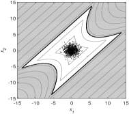
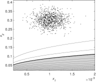
Figure 1: Contour plots of $f$ in Example 4.1.1 (left) and Example 4.1.2 (right), along with a sample of size $m=10^{3}$ from $\mathsf{P}_{\mathds{X}}$ (dots). A failure happens when $x$ is in the gray area.

4.1.2 Deviation of a cantilever beam

Consider a cantilever beam, with a rectangular cross-section, subjected to a uniform load. The deflection of the tip of the beam can written as

(23) $$f(x_{1},x_{2})=\frac{3L^{4}}{2E}\frac{x_{1}}{x_{2}^{3}}\,,$$

where $x_{1}$ is the load per unit area, $x_{2}$ the thickness of the beam, $L=6\,{\rm m}$ and $E=2.6\!\cdot\!10^{4}\,{\rm MPa}$. The input variable $X_{1}$ and $X_{2}$ are assumed independent, with $X_{1}\sim\mathcal{N}\bigl{(}\mu_{1},\sigma_{1}^{2})$, $\mu_{1}=10^{-3}\,{\rm MPa}$, $\sigma_{1}=0.2\mu_{1}$, and $X_{2}\sim\mathcal{N}\bigl{(}\mu_{2},\sigma_{2}^{2}\bigr{)}$, $\mu_{2}=0.3\,{\rm m}$, $\sigma_{2}=0.1\mu_{2}$. A failure occurs when $f$ is larger than $u=L/325$. The probability of failure is approximately $3.937\!\cdot\!10^{-6}$, with a coefficient of variation of about $0.03\%$. Note that the distribution of $X_{2}$ has been modified, with respect to the usual formulation (see, e.g., [35]), to make $\alpha$ smaller. Figure 1 (right panel) shows a contour plot of $f$, along with a sample of the input distribution.

4.1.3 Response of a nonlinear oscillator

In this example (see, e.g., [31]), the input variable is six-dimensional and the cost function is:

(24) $$f\left(x_{1},x_{2},x_{3},x_{4},x_{5},x_{6}\right)=3x_{4}-\left\lvert\frac{2x_{5}}{x_{1}{w_{0}}^{2}}\sin\Big{(}\frac{w_{0}x_{6}}{2}\Big{)}\right\rvert$$

where $w_{0}=\sqrt{\frac{x_{2}+x_{3}}{x_{1}}}$. The input variables are assumed independent, normal, with mean and variance parameters given in Table 4. A failure happens when the cost function is lower than the threshold $u=0$. The probability of failure is approximately $1.514\!\cdot\!10^{-8}$, with a coefficient of variation of about $0.04\%$. This variant of the problem corresponds exactly to the harder case in [31].

Table 4: Example 4.1.3: Means and standard deviations of the input variables.

Variable	$x_{1}$	$x_{2}$	$x_{3}$	$x_{4}$	$x_{5}$	$x_{6}$
$\mu_{i}$	$1$	$1$	$0.1$	$0.5$	$0.45$	$1$
$\sigma_{i}$	$0.05$	$0.1$	$0.01$	$0.05$	$0.075$	$0.2$

4.2 Experimental settings

4.2.1 BSS algorithm

Initial design of experiments

We start with an initial design of size $n_{0}=5d$ (see [43] for a discussion on the size of the initial design in computer experiments), generated as follows. First, a compact subset $\mathds{X}_{0}\subset\mathds{X}$ is constructed:

$$\mathds{X}_{0}=\prod_{j=1}^{d}\left[q_{\varepsilon}^{j};q_{1-\varepsilon}^{j}\right]$$

where $q_{\varepsilon}^{j}$ and $q_{1-\varepsilon}^{j}$ are the quantiles of order $\varepsilon$ and $1-\varepsilon$ of the $j^{\text{th}}$ input variable. Then, a “good” LHS design on $\left[0;1\right]^{d}$ is obtained as the best design according the maximin criterion [38, 45] in a set of $Q$ random LHS designs, and then scaled to $\mathds{X}_{0}$ using an affine mapping. The values $\varepsilon=10^{-5}$ and $Q=10^{4}$ have been used in all our experiments.

Stochastic process prior

A Gaussian process prior with an unknown constant mean and a stationary anisotropic Matérn covariance function with regularity $5/2$ is used as our prior information about $f$ (see Supplementary Material SM2 for more details). The unknown mean is integrated out as usual, using an improper uniform prior on $\mathds{R}$; as a consequence, the posterior mean coincides with the so-called “ordinary kriging” predictor. The remaining hyper-parameters (variance and range parameters of the covariance function) are estimated, following the empirical Bayes philosophy, by maximization of the marginal likelihood. The hyper-parameters are estimated first on the data from the initial design, and then re-estimated after each new evaluation. In practice, we recommend to check the estimated parameters every once in a while using, e.g., leave-one-out cross-validation.

SMC parameters

Several values of the sample size $m$ will be tested to study the relation between the variance of the estimator and the number of evaluations: $m\in\{500,1000,2000,\ldots\}$. Several iterations of an adaptive Gaussian Random Walk Metropolis-Hastings (RWMH) algorithm, fully described in Supplementary Material SM3, are used for the move step of the algorithm.

Stopping criterion for the SUR strategy

The number of evaluations selected using the SUR strategy is determined adaptively, using the stopping criterion (21) from Section 3.5, with $\eta_{t}=0.5$ for all $t<T$ (i.e., for all intermediate stages) and $\eta_{T}=0.1\,\widehat{\delta}_{m,T}$ where $\widehat{\delta}_{m,T}$ is the estimated coefficient of variation for the SMC estimator $\mskip 1.0mu\widehat{\vphantom{\rule{1.0pt}{5.71527pt}}\smash{\mskip-1.0mu\widehat{\alpha}}}^{\mskip 1.0mu\text{\tiny BSS}}_{T}$ of $\widehat{\alpha}^{\mskip 1.0mu\text{\tiny B}}_{T}$ (see Appendix A). Furthermore, we require for robustness a minimal number $N_{\text{min}}$ of evaluations at each stage, with $N_{\text{min}}=2$ in all our simulations.

Adaptive choice of the thresholds

The successive thresholds $u_{t}$ are chosen using the adaptive rule proposed in Section 3.4, Equation (20), with $p_{0}=0.1$. This value has been found experimentally to be neither too large (to avoid having a large number of stages) not too small (to avoid losing too many particles during the resampling step).

4.2.2 Subset simulation algorithm

The parameters used for the subset simulation algorithm are exactly the same, in all our simulations, as those used in the “SMC part” of the BSS algorithm (see Section 4.2.1). In particular, the number $m_{0}$ of surviving particles at each stage is determined according to the rule $p_{0}=\frac{m_{0}}{m}=0.1$ (see Table 1), and the adaptive MCMC algorithm described in Supplementary Material SM3 is used to move the particles. The number of evaluations made by the subset simulation algorithm is considered to be $m+\left(T-1\right)\left(1-p_{0}\right)m$, as explained in Section 2.4—in other words, in order to make the comparison as fair as possible, the additional evaluations required by the adaptive MCMC procedure are not taken into account.

4.2.3 ²SMART algorithm

²SMART [10, 20] is another algorithm for the estimation of small probabilities, which is based on the combination of subset simulation with Support Vector Machines (SVM). We will present results obtained using the implementation of ²SMART proposed in the software package FERUM 4.1 [8], with all parameters set to their default values (which are equal to the values given in [10]).

Remark 10.

Several other methods addressing the estimation of small probabilities of failure for expensive-to-evaluate functions have appeared recently in the structural reliability literature [4, 9, 12, 31, 37]. ²SMART was selected as a reference method due to the availability of a free software implementation in FERUM. A more comprehensive benchmark is left for future work.

4.3 Results

4.3.1 Illustration

We first illustrate how BSS works using one run of the algorithm on Example 4.1.1 with sample size $m=1000$. Snapshots of the algorithm at stages $t=1$, $t=5$ and $t=T=9$ are presented on Figure 2. Observe that the additional evaluation points selected at each stage using the SUR criterion (represented by black triangles) are located in the vicinity of the current level set. The actual number of points selected at each stage, determined by the adaptive stopping rule, is reported in Table 5. Observe also that the set of particles (black dots in the right column) is able to effectively capture the bimodal target distribution. Finally, observe that a significant portion of the evaluation budget is spent on the final stage—this is again a consequence of our adaptive stopping rule, which refines the estimation of the final level set until the bias of the estimate is (on average under the posterior distribution) small compared to its standard deviation.

Figure 2: Snapshots of the BSS algorithm running on Example 4.1.1 (four branch series system) with sample size $m=1000$. The first, second and third row correspond respectively to the end of the first stage ($t=1$), the fifth stage ($t=5$) and the last stage ($t=T=9$). The true level set corresponding current target level $u_{t}$ is represented by a thick line and, in the left column, true level sets corresponding to previous levels ($u_{s}$, $s<t$) are recalled using dashed contours. Evaluation points from previous stages are represented by gray disks (in particular, the initial design of experiment of size $n_{0}=10$ is visible on the top-left panel) and new evaluations performed at the current levels are marked by black triangles. In the right column, the sample points $Y_{t-1}^{j}$, $1\leq j\leq m$ and the level sets of the input density $\pi_{\mathds{X}}$ (corresponding to probabilities $1-10^{-k}$, $k=1,2,\ldots$) are represented respectively by black dots and dotted lines.

Table 5: Number of evaluations per stage on Example 4.1.1 (four-branch series system). For the BSS algorithm, recall that the number of evaluations at each stage is chosen adaptively (see Section 3.5) and is therefore random: the numbers shown here correspond to the run with $m=1000$ that is shown on Figure 2. For the subset simulation algorithm, the number of evaluations is directly related to the $m$, $q_{0}=1-p_{0}$ and $T$ (see Section 2.4).

stage number $t$	$0$	$1$	$2$	$3$	$4$	$5$
BSS ($m=1000$)	$2d=10$	$2$	$6$	$3$	$2$	$3$
subset simulation	$m$	$q_{0}m$	$q_{0}m$	$q_{0}m$	$q_{0}m$	$q_{0}m$

stage number $t$	$6$	$7$	$8$	$9$	total
BSS ($m=1000$)	$2$	$3$	$2$	$28$	$61$
subset simulation	$q_{0}m$	$q_{0}m$	$q_{0}m$	0	$m+(T-1)q_{0}m$

4.3.2 Average results

This section presents average results over one hundred independent runs for subset simulation, BSS and ²SMART.

Figure 3 represents the average number of evaluations used by the BSS algorithm as a function of the sample size $m$. The number of evaluations spent on the initial design is constant, since it only depends on the dimension $d$ of the input space. The average number of evaluations spent on the intermediate stages ($t<T$) is also very stable and independent of the sample size $m$. Only the average number of evaluations spent on the final stage—i.e., to learn the level set of interest—is growing with $m$. This growth is necessary if one wants the estimation error to decrease when $m$ increases: indeed, the variance of $\mskip 1.0mu\widehat{\vphantom{\rule{1.0pt}{5.71527pt}}\smash{\mskip-1.0mu\widehat{\alpha}}}^{\mskip 1.0mu\text{\tiny BSS}}_{T}$ automatically goes to zero at the rate $\frac{1}{m}$, but the bias $\widehat{\alpha}^{\mskip 1.0mu\text{\tiny B}}_{T}-\alpha$ does not unless additional evaluations are added at the final level to refine the estimation of $\Gamma$.

Figure 4 represents the relative Root-Mean-Square Error (RMSE) of all three algorithms, as a function of the average number of evaluations. For the subset simulation algorithm, the number of evaluations is directly proportional to $m$ and the RMSE decreases as expected like $\frac{1}{m}$ (with a constant much smaller than that of plain Monte Carlo simulation). ²SMART clearly outperforms subset simulation, but offers no simple way of tuning the accuracy of the final estimate (which is why only one result is presented, using the default settings of the algorithm). Finally, BSS clearly and consistently outperforms both ²SMART and subset simulation on these three examples: the relative RMSE goes to zero at a rate much faster than subset simulation’s (a feature that is made possible by the smoothness of the limit-state function, which is leveraged by the Gaussian process model), and the sample size $m$ is the only tuning parameters that needs to be acted upon in order change the accuracy of the final estimate. Figure 5 provides more insight into the error of the BSS estimate by confirming that, as intended by design of the adaptive stopping rule, variance is the main component of the RMSE (in other words, the bias is negligible in these examples).

Finally, note that the BSS estimation involves a computational overhead with respect to subset simulation. A careful analysis of the run times of BSS on the three examples (provided as Supplementary Material SM4.1) reveals that the computational overhead of BSS is approximately equal to $C_{0}+C_{1}\,m\,N_{\mathrm{SUR}}$, where $N_{\mathrm{SUR}}$ the total number of evaluations selected using the SUR criterion (i.e., all evaluations except the initial design of experiments). This shows that, in our implementation, the most time-consuming part of the algorithm is the selection of additional evaluation points using the SUR criterion. However, in spite of its computational overhead, BSS is preferable to the subset simulation algorithm in terms of computation time, on the three test cases, as soon as the evaluation time $\tau_{\text{sim}}$ of $f$ is large enough—larger than, say, 10 ms for the considered range of relative RMSE (see Supplementary Material SM4.2 for details). Consider for instance Example 4.1.1 with $\tau_{\mathrm{sim}}=1\,s$: BSS with sample size $m=8000$ achieves a relative RMSE of approximately $10\%$ in about 3 minutes while subset simulation requires about 19 hours to achieve a comparable accuracy.

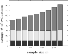
(a) Example 4.1.1: Four branch

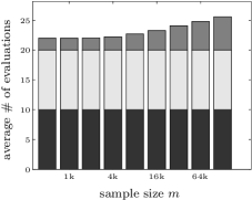
(b) Example 4.1.2: Cantilever beam

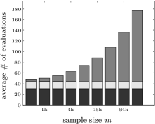
(c) Example 4.1.3: Nonlinear oscillator

Figure 3: Average number of evaluations used by the BSS algorithm, over 100 independent runs, as a function of the sample size $m$ on Examples 4.1.1–4.1.3. The total number of evaluations is split in three parts: the size $n_{0}$ of the initial design (dark gray), the number $\sum_{t=1}^{T-1}N_{t}$ of evaluations in intermediate stages (light gray) and the number of evaluations $N_{T}$ in the final stage (middle gray).

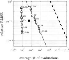
(a) Example 4.1.1: Four branch

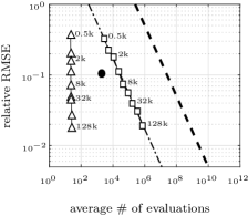
(b) Example 4.1.2: Cantilever beam

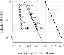
(c) Example 4.1.3: Nonlinear oscillator

Figure 4: Relative root-mean-square error (RMSE) as a function of the average number of evaluations, over 100 independent runs, on Examples 4.1.1–4.1.3. For the subset simulation algorithm (squares) and for the BSS algorithm (triangles), the results are provided for several values of the sample size ($m\in\{500,1000,2000,\ldots\}$). For the ²SMART algorithm (filled circles), only one result is presented, corresponding to the default settings of the algorithm. The expected performance of plain Monte Carlo sampling is represented by a dashed line. The mixed line represents a simple approximation of the relative RMSE for the subset simulation algorithm: $\frac{T_{\alpha}}{m}\,\frac{1-p_{0}}{p_{0}}$, where $T_{\alpha}=\lceil\frac{\log\alpha}{\log p_{0}}\rceil$.

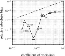
(a) Example 4.1.1: Four branch

(b) Example 4.1.2: Cantilever beam

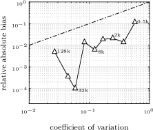
(c) Example 4.1.3: Nonlinear oscillator

Figure 5: Relative absolute bias of the BSS estimator as a function of its coefficient of variation, estimated using 100 independent runs. The relative absolute bias is estimated using, for each test case, the reference value $\alpha_{\text{ref}}$ provided in Table 3.

5 Discussion

We propose an algorithm called Bayesian subset simulation for the estimation of small probabilities of failure—or more generally the estimation of the volume of excursion of a function above a threshold—when the limit-state function is expensive to evaluate. This new algorithm is built upon two key techniques: the SMC method known as subset simulation or adaptive multilevel splitting on the one hand, and the Bayesian (Gaussian process based) SUR sampling strategy on the other hand. SMC simulation provides the means for evaluating the Bayesian estimate of the probability of failure, and to evaluate and optimize the SUR sampling criterion. In turn, the SUR sampling strategy makes it possible to estimate the level sets of the (smooth) limit-state function using a restricted number of evaluations, and thus to build a good sequence of target density for SMC simulation. Our numerical experiments show that this combination achieves significant savings in evaluations on three classical examples from the structural reliability literature.

An adaptive stopping rule is used in the BSS algorithm to choose the number of evaluation added by the SUR sampling strategy at each stage. Evaluations at intermediate stages are not directly useful to refine the final probability estimate, but their importance must not be overlooked: they make it possible to learn in a robust way the level sets of the limit-state function, and therefore to build a sequence of densities that converges to the boundary of the failure region. Achieving a better understanding of the connection between the number of evaluations spent on intermediate level sets and the robustness of the algorithm is an important perspective for future work. In practice, if the budget of evaluations permits, we recommend running several passes of the BSS algorithm, with decreasing tolerances for the adaptive stopping rule, to make sure that no failure mode has been missed.

The adaptive stopping rule also makes it possible to refine the estimation of the final level set to make sure that the posterior model is good enough with respect to the SMC sample size. Other settings of the stopping rule could of course be considered. For instance, BSS could stop when the bias is expected to be of the same order as the standard deviation. Future work will focus on fully automated variants on the BSS algorithm, where the number of evaluations and the SMC sample size would be controlled in order to achieve a prescribed error level.

Appendix A Computation of the variance in the idealized setting

This section provides a derivation of Equations (17) and (18), together with an explicit expression of the estimated coefficient of variation $\widehat{\delta}_{m,T}$ used in Section 4.2.1. Both are obtained in the setting of the idealized BSS algorithm described in Section 3.4, where the samples $\mathds{Y}_{t}=\left\{Y_{t}^{1},\,\ldots,\,Y_{t}^{m}\right\}$ are assumed IID (with density $q_{t}$) and mutually independent.

Recall from Equation (16) that the BSS estimator can be written as

(25) $$\mskip 1.0mu\widehat{\vphantom{\rule{1.0pt}{5.71527pt}}\smash{\mskip-1.0mu\widehat{\alpha}}}^{\mskip 1.0mu\text{\tiny BSS}}_{T}\;=\;\prod_{t=1}^{T}\frac{\mskip 1.0mu\widehat{\vphantom{\rule{1.0pt}{5.71527pt}}\smash{\mskip-1.0mu\widehat{\alpha}}}^{\mskip 1.0mu\text{\tiny BSS}}_{t}}{\mskip 1.0mu\widehat{\vphantom{\rule{1.0pt}{5.71527pt}}\smash{\mskip-1.0mu\widehat{\alpha}}}^{\mskip 1.0mu\text{\tiny BSS}}_{t-1}}\;=\;\prod_{t=1}^{T}\left(\frac{1}{m}\,\sum_{j=1}^{m}\frac{g_{t}(Y_{t-1}^{j})}{g_{t-1}(Y_{t-1}^{j})}\right)\;=\;\prod_{t=1}^{T}\,\mskip 3.0mu\widehat{\vphantom{\rule{1.0pt}{5.71527pt}}\smash{\mskip-3.0mu\widehat{p}}}^{\mskip 3.0mu\text{\tiny BSS}}_{t}\,,$$

where we have set, for all $t\in\{1,\,\ldots,\,T\}$,

$$\mskip 3.0mu\widehat{\vphantom{\rule{1.0pt}{5.71527pt}}\smash{\mskip-3.0mu\widehat{p}}}^{\mskip 3.0mu\text{\tiny BSS}}_{t}=\frac{1}{m}\,\sum_{j=1}^{m}\frac{g_{t}(Y_{t-1}^{j})}{g_{t-1}(Y_{t-1}^{j})}.$$

Observe that the random variables $\mskip 3.0mu\widehat{\vphantom{\rule{1.0pt}{5.71527pt}}\smash{\mskip-3.0mu\widehat{p}}}^{\mskip 3.0mu\text{\tiny BSS}}_{t}$ are independent, with mean

$$\mathsf{E}\left(\mskip 3.0mu\widehat{\vphantom{\rule{1.0pt}{5.71527pt}}\smash{\mskip-3.0mu\widehat{p}}}^{\mskip 3.0mu\text{\tiny BSS}}_{t}\right)=\int_{\mathds{X}}\frac{g_{t}}{g_{t-1}}\,q_{t-1}=\int_{\mathds{X}}\frac{g_{t}}{g_{t-1}}\,\frac{g_{t-1}\,\pi_{\mathds{X}}}{\widehat{\alpha}^{\mskip 1.0mu\text{\tiny B}}_{t-1}}=\frac{\widehat{\alpha}^{\mskip 1.0mu\text{\tiny B}}_{t}}{\widehat{\alpha}^{\mskip 1.0mu\text{\tiny B}}_{t-1}}=\widehat{p}^{\mskip 3.0mu\text{\tiny B}}_{t}$$

and variance

$$\operatorname{var}\left(\mskip 3.0mu\widehat{\vphantom{\rule{1.0pt}{5.71527pt}}\smash{\mskip-3.0mu\widehat{p}}}^{\mskip 3.0mu\text{\tiny BSS}}_{t}\right) =\frac{1}{m}\,\operatorname{var}\left(\frac{g_{t}\left(Y_{t-1}^{1}\right)}{g_{t-1}\left(Y_{t-1}^{1}\right)}\right)$$

$$=\frac{1}{m}\,\left[\int_{\mathds{X}}\frac{g_{t}^{2}}{g_{t-1}^{2}}\,\frac{g_{t-1}\,\pi_{\mathds{X}}}{\widehat{\alpha}^{\mskip 1.0mu\text{\tiny B}}_{t-1}}-\left(\frac{\widehat{\alpha}^{\mskip 1.0mu\text{\tiny B}}_{t}}{\widehat{\alpha}^{\mskip 1.0mu\text{\tiny B}}_{t-1}}\right)^{2}\right]$$

$$=\frac{1}{m}\,\left[\frac{1}{\widehat{\alpha}^{\mskip 1.0mu\text{\tiny B}}_{t-1}}\,\int_{\mathds{X}}\frac{g_{t}^{2}}{g_{t-1}}\,\pi_{\mathds{X}}-\left(\frac{\widehat{\alpha}^{\mskip 1.0mu\text{\tiny B}}_{t}}{\widehat{\alpha}^{\mskip 1.0mu\text{\tiny B}}_{t-1}}\right)^{2}\right]$$

$$=\frac{1}{m}\,\left(\widehat{p}^{\mskip 3.0mu\text{\tiny B}}_{t}\right)^{2}\kappa_{t},$$

where $\kappa_{t}$ is defined by (18). Therefore, the coefficients of variation $\delta_{m,t}$ of the sequence of estimators $\mskip 1.0mu\widehat{\vphantom{\rule{1.0pt}{5.71527pt}}\smash{\mskip-1.0mu\widehat{\alpha}}}^{\mskip 1.0mu\text{\tiny BSS}}_{t}$ obey the recurrence relation $\delta_{m,t}^{2}=\frac{1}{m}\kappa_{t}+\left(1+\frac{1}{m}\kappa_{t}\right)\,\delta_{m,t-1}^{2}$, and we conclude that

$$\delta_{m,T}^{2} =\frac{1}{m}\kappa_{T}+\left(1+\frac{1}{m}\kappa_{T}\right)\,\frac{1}{m}\kappa_{T-1}$$

$$\quad+\left(1+\frac{1}{m}\kappa_{T}\right)\,\left(1+\frac{1}{m}\kappa_{T-1}\right)\,\frac{1}{m}\kappa_{T-2}+\cdots$$

$$=\frac{1}{m}\sum_{t=1}^{T}\kappa_{t}+O\left(\frac{1}{m^{2}}\right),$$

which proves Equations (17)–(18). We construct an estimator of the coefficient of variation recursively, using the relation

$$\widehat{\delta}_{m,t}^{2}=\frac{1}{m}\widehat{\kappa}_{t}+\left(1+\frac{1}{m}\widehat{\kappa}_{t}\right)\,\widehat{\delta}_{m,t-1}^{2},$$

with

$$\widehat{\kappa}_{t}=\left(\mskip 3.0mu\widehat{\vphantom{\rule{1.0pt}{5.71527pt}}\smash{\mskip-3.0mu\widehat{p}}}^{\mskip 3.0mu\text{\tiny BSS}}_{t}\right)^{-2}\,\cdot\,\frac{1}{m}\sum_{j=1}^{m}\left(\frac{g_{t}\left(Y_{t-1}^{j}\right)}{g_{t-1}\left(Y_{t-1}^{j}\right)}-\mskip 3.0mu\widehat{\vphantom{\rule{1.0pt}{5.71527pt}}\smash{\mskip-3.0mu\widehat{p}}}^{\mskip 3.0mu\text{\tiny BSS}}_{t}\right)^{2}.$$

SUPPLEMENTARY MATERIALS

Appendix SM1 Approximation and optimization of the SUR criterion

This section discusses the numerical procedure that we use for the approximation and optimization of the SUR criterion used at each stage of the BSS algorithm (see Sections 3.1 and 3.3):

$$J_{n}\left(x_{n+1}\right)\;=\;\int_{\mathds{X}}\mathsf{E}_{n,x_{n+1}}\left(\tau_{n+1,u_{t}}(x)\right)\,\pi_{\mathds{X}}(x)\,\mathrm{d}x,\qquad n_{t-1}\leq n\leq n_{t}-1,$$

where we have introduced the simplified notation $\mathsf{E}_{n,x_{n+1}}\mathrel{\coloneqq}\mathsf{E}_{n}\left(\,\cdot\;\big{\lvert}\;X_{n+1}=x_{n+1}\right)$. The numerical approach proposed here is essentially the same as that used by [6], with a more accurate way of computing the integrand, following ideas of chevalier:SM.

Observing that

$$J_{n}\left(x_{n+1}\right)\;=\;\widehat{\alpha}^{\mskip 1.0mu\text{\tiny B}}_{t-1}\,\int_{\mathds{X}}\frac{\mathsf{E}_{n,x_{n+1}}\left(\tau_{n+1,u_{t}}(x)\,\right)}{g_{t-1}(x)}\,q_{t-1}(x)\,\mathrm{d}x,$$

the integral over $\mathds{X}$ can be approximated, up to a constant, using the weighted sample $\mathds{Y}_{t-1}$:

$$J_{n}\left(x_{n+1}\right) \;\propto\;\int_{\mathds{X}}\frac{\mathsf{E}_{n,x_{n+1}}\left(\tau_{n+1,u_{t}}(x)\right)}{g_{t-1}(x)}\,q_{t-1}(x)\,\mathrm{d}x$$

(SM1) $$\;\approx\;\sum_{j=1}^{m}w_{t-1}^{j}\,\frac{\mathsf{E}_{n,x_{n+1}}\left(\tau_{n+1,u_{t}}(x)\right)_{|x=Y_{t-1}^{j}}}{g_{t-1}\left(Y_{t-1}^{j}\right)}.$$

Then, simple computations using well-known properties of Gaussian processes under conditioning allow to obtain an explicit representation of the integrand, in the spirit of chevalier:SM, as a function of the Gaussian process posterior mean $\widehat{\xi}_{n}$ and posterior covariance $k_{n}$:

$$\mathsf{E}_{n,x_{n+1}} \left(\tau_{n+1,u_{t}}(x)\right)\;=\;\Phi\left(\frac{u-\widehat{\xi}_{n}(x)}{\sigma_{n}(x)}\right)+\Phi\left(\frac{u-\widehat{\xi}_{n}(x)}{s_{n}(x,x_{n+1})}\right)$$

(SM2) $$\qquad-2\,\Phi_{2}\left(\begin{pmatrix}u\\ u\end{pmatrix};\,\begin{pmatrix}\widehat{\xi}_{n}(x)\\ \widehat{\xi}_{n}(x)\end{pmatrix},\,\begin{pmatrix}s_{n}^{2}(x,x_{n+1})&s_{n}^{2}(x,x_{n+1})\\ s_{n}^{2}(x,x_{n+1})&\sigma_{n}(x)^{2}\end{pmatrix}\right),$$

where $\Phi$ is the cumulative distribution function of the normal distribution, $\Phi_{2}$ the cumulative distribution function of the bivariate normal distribution, $\sigma_{n}^{2}(x)=k_{n}(x,x)$ and $s_{n}^{2}(x,x_{n+1})=k_{n}(x,x_{n+1})^{2}/\sigma_{n}(x_{n+1})^{2}$.

The main computational bottleneck, in a direct implementation of the approximation (SM1) combined with the representation (SM2), is in our experience the computation of the bivariate cumulative distribution function $\Phi_{2}$. Indeed, assume that the optimization of the approximate criterion is carried out by means of an exhaustive discrete search on $\{Y_{t-1}^{j},1\leq j\leq m\}$. Then $m^{2}$ evaluations of $\Phi_{2}$ are required in order select $X_{n+1}$. To mitigate this problem, we implemented the pruning idea proposed in Section 3.4 of [6]: only a subset of size $m_{0}\leq m$ of the set of particles is actually used, both for the approximation the integral and for the optimization of the criterion. In this article, the size $m_{0}$ is determined automatically as follows: first, for each particle $Y_{t-1}^{j}$, the current weighted probability of misclassification

$$\widetilde{\tau}_{n}^{j}\mathrel{\coloneqq}w_{t-1}^{j}\tau_{n,u_{t}}\left(Y_{t-1}^{j}\right)/g_{t-1}\left(Y_{t-1}^{j}\right)$$

is computed. Then, the particules are sorted according to the value of $\widetilde{\tau}_{n}^{j}$, in decreasing order: $\widetilde{\tau}_{n}^{\varphi(1)}\;\geq\;\widetilde{\tau}_{n}^{\varphi(2)}\;\geq\;\ldots\geq\widetilde{\tau}_{n}^{\varphi(m)}$, and $m_{0}$ is set to $\min\left(m_{0}^{\text{max}},m_{0}(\widetilde{\tau}_{n})\right)$, where $m_{0}(\widetilde{\tau}_{n})$ is the smallest integer such that

$$\sum_{j=1}^{m_{0}}\widetilde{\tau}_{n}^{\varphi(j)}\;\geq\;\rho\,\sum_{j=1}^{m}\widetilde{\tau}_{n}^{j}.$$

The values $m_{0}^{\text{max}}=1000$ and $\rho=0.99$ have been used in all our simulations.

Appendix SM2 Stochastic process prior

The stochastic process prior used for the numerical experiments in this article is a rather standard Gaussian process model. We describe it here in full detail for the sake of completeness. First, $\xi$ is written as

$$\xi(x)=\mu+\xi^{0}(x),$$

where $\mu\in\mathds{R}$ is an unknown constant mean and $\xi^{0}$ a zero-mean stationary Gaussian process with anisotropic covariance function

(SM3) $$k(x,y)=\sigma^{2}\kappa_{\nu}\left(\sqrt{\sum_{i=1}^{d}\frac{(x_{[i]}-y_{[i]})^{2}}{\rho_{i}^{2}}}\right)\,,\quad x,y\in\mathds{R}^{d},$$

where $x_{[i]},y_{[i]}$ denote the $i^{\rm th}$ coordinate of $x$ and $y$, and $\kappa_{\nu}$ the Matérn correlation function of regularity $\nu$ (see Ste99:SM, Section 2.10). The scale parameters $\rho_{1}$, …, $\rho_{d}$ (characteristic correlation lengths) are usually called the range parameters of the covariance function.

In this article, the regularity parameter $\nu$ is set to the fixed value $\nu=5/2$, leading to the following analytical expression for the Matérn correlation function:

(SM4) $$\kappa_{\nu}\left(h\right)=\left(1+\tilde{h}+\frac{1}{3}\tilde{h}^{2}\right)\,\exp\left(-\tilde{h}\right),\qquad\text{with }\tilde{h}=\sqrt{10}\,\left|h\right|.$$

As a consequence, $\xi$ is twice differentiable in the mean-square sense, with sample paths almost surely in the Sobolev space $W^{s,2}$ for all $s<5/2$ (scheuerer2010regularity, Theorem 3).

Remark SM1.

The parameterization used in Equation (SM4) is the one advocated in Ste99:SM. Other parameterizations are sometimes used in the literature; e.g., rasmussenWilliams use $\tilde{h}=\sqrt{5}\,\left|h\right|$.

Appendix SM3 Adaptive Metropolis-Hastings algorithm for the move step

A fixed number $S$ of iterations of a Gaussian Random Walk Metropolis-Hastings (RWMH) kernel is used for the move step, with adaptation of the standard deviations of the increments. More precisely, for $s=1,2,\ldots,S$, starting with the set of particles $\left(Y_{t,1}^{(j)}\right)_{1\leq j\leq m}$ produced by the resampling step, we first produce perturbed particles:

$$\widetilde{Y}_{t,s}^{(j)}=Y_{t,s}^{(j)}+\Sigma_{\text{RW},t,s}\,U_{t,s},\qquad 1\leq j\leq m,$$

where $\Sigma_{\text{RW},t,s}$ is a diagonal matrix and $U_{t,s}$ a $d$-dimensional standard normal vector. The perturbed particle is accepted as $Y_{t,s+1}^{(j)}$ with probability

$$a_{t,s}^{(j)}=1\wedge\frac{q_{t}\left(\widetilde{Y}_{t,s}^{(j)}\right)}{q_{t}\left(Y_{t,s}^{(j)}\right)},$$

and $Y_{t,s}^{(j)}$ is kept otherwise. The $k^{\text{th}}$ diagonal element $\sigma_{\text{RW},t,s}^{(k)}$ of $\Sigma_{\text{RW},t,s}$ is initialized with

(SM5) $$\sigma_{\text{RW},1,1}^{(k)}=C_{\sigma,\text{init}}\,\sigma_{\mathds{X}}^{(k)},$$

where $\sigma_{\mathds{X}}^{(k)}$ is the standard deviation of the $k^{\text{th}}$ marginal of $\mathsf{P}_{\mathds{X}}$, and then updated using

(SM6) $$\log\sigma_{\text{RW},t,s}^{(k)}=\begin{cases}\log\sigma_{\text{RW},t,s-1}^{(k)}+\Delta_{\sigma}/s&\text{if }\bar{a}_{t,s}>a_{\text{target}}\\ \log\sigma_{\text{RW},t,s-1}^{(k)}-\Delta_{\sigma}/s&\text{otherwise,}\end{cases}$$

where $\sigma_{\text{RW},t,-1}^{(k)}=\sigma_{\text{RW},t-1,S}^{(k)}$, $\bar{a}_{t,s}=\frac{1}{m}\sum_{j=1}^{m}a_{t,s}^{(j)}$ is the average acceptance probability and $a_{\text{target}}$ some prescribed target value.

The following parameter values have been used for the numerical simulations presented in this article: $S=10$, $C_{\sigma,\text{init}}=2/\sqrt{d}$, $\Delta_{\sigma}=\log(2)$ and $a_{\text{target}}=30\%$.

Remark SM2.

The $1/\sqrt{d}$ scaling for the constant $C_{\sigma,\text{init}}$ in (SM5) is motivated by the well-known theorem of roberts1997weak, which provides the optimal covariance matrix $2.38^{2}\Sigma/d$ for a Gaussian target with covariance matrix $\Sigma$ in high dimension.

Remark SM3.

The value $\Delta_{\sigma}=\log(2)$ that was used in the simulation turns out to be too small to be a good general recommendation for a default value. Indeed, with $S=10$ steps of adaptation, it leads to a maximal adaptation factor of $2^{1+\frac{1}{2}+\ldots+\frac{1}{10}}\approx 7.6$, which might prove too small for some cases. The value $\Delta_{\sigma}=\log(10)$ is thus used as a default value in the Matlab/Octave program that is provided as Supplementary Material.

Remark SM4.

The reader is referred to vihola2010convergence and references therein for more information on adaptive MCMC algorithms, including adaptive scaling algorithms such as (SM6). Note, however, that the adaptation scheme proposed here is not strictly-speaking an adaptive MCMC scheme, since we use the entire population of particles to estimate the acceptance probability.

Remark SM5.

Our adaptive scheme (SM5)–(SM6) is admittedly very simple, but works well in the examples of the paper. More refined adaptation schemes might be needed to deal with harder problems. For instance, it might become necessary to implement a truly anisotropic adaptation of the covariance matrix, or to use different kernels in different regions of the input space. Ideas from the adaptive SMC literature (see, e.g., fearnhead2013adaptive, cornebise2008, chang2003optim) could be leveraged to achieve these goals, which fall out of the scope of the present paper.

Appendix SM4 Run time of the BSS algorithm

SM4.1 Overhead of the BSS algorithm

The median run times of the Bayesian subset simulation (BSS) and subset simulation (SS) algorithms on the three test cases of Section 4 are reported in Table SM1. Since the function $f$ in each of these examples is actually very fast to evaluate, these run times provide a good indication of the numerical complexity of the algorithms. Consequently, they provide a measure of the overhead of the algorithm if it were actually run on an expensive-to-evaluate function (i.e., the fraction of the computation time not dedicated to evaluating the function).

As expected, because of the computations related to Gaussian process modeling, the overhead of BSS is larger than the one of subset simulation, for a given sample size $m$. In our implementation, this overhead, which we denote by $\tau_{\text{BSS},0}$, can be explained by a simple linear model:

(SM7) $$\tau_{\text{BSS},0}\;\approx\;C_{0}+C_{1}mN_{\text{SUR}}$$

where $m$ is the sample size and $N_{\text{SUR}}$ the total number of evaluations selected using the SUR criterion (i.e., all evaluations except the initial design of experiments). On our standard Intel-Nehalem-based workstation, an ordinary least-square regression using Equation (SM7), on the $100\times 3\times 8=2400$ points of our data set (100 runs on 3 cases with 8 sample sizes), yields $C_{0}\approx 27.0$ and $C_{1}\approx 5.2\,10^{-5}$, with a coefficient of determination of $97.2\%$. We conclude that the most time-consuming part of the algorithm is the selection of additional evaluation points using the SUR criterion.

Remark SM6.

Note that the computation time of BSS would grow as a function of $m^{2}\,N_{\text{SUR}}$, instead of $m\,N_{\text{SUR}}$, without the pruning idea explained in Section A.

SM4.2 Extrapolation to expensive-to-evaluate functions

Let us now extrapolate from the available data, obtained for cheap-to-evaluate test functions, to the case of a non-negligible evaluation time. To this end, assume that each evaluation actually costs $\tau_{\text{sim}}$ in computation time. Then, the total run time of BSS becomes

(SM8) $$\tau_{\text{BSS}}\;=\;\tau_{\text{BSS},0}+\tau_{\text{sim}}\,N,$$

where $N$ is the total number of evaluations. For a given test case and a given sample size $m$, denote by $\bar{N}$ the average total number of evaluation, $\bar{\tau}_{\text{BSS},0}$ the average overhead and rRMSE the relative root-mean-square error (computed using 100 runs of BSS). The efficiency of BSS with respect to the subset simulation algorithm can be measured by the ratio

(SM9) $$\varepsilon_{\text{BSS}\,|\,\text{SS}}\;=\;\frac{\tau_{\text{SS}}}{\bar{\tau}_{\text{BSS}}}$$

where $\bar{\tau}_{\text{BSS}}=\bar{\tau}_{\text{BSS},0}+\tau_{\text{sim}}\,\bar{N}$ is the average total run time for BSS, and $\tau_{\text{SS}}$ is an approximation of the time it would take for subset simulation to reach the same relative RMSE, computed as:

(SM10) $$\tau_{\mathrm{SS}}=\tau_{\text{sim}}\,m\,\left(1+(T_{\alpha}-1)(1-p_{0})\right),$$

where $T_{\alpha}=\lceil\frac{\log\alpha}{\log p_{0}}\rceil$ and $m$ is the sample size that gives the same relative RMSE according to the relation

(SM11) $$\text{rRMSE}\;\approx\;\frac{T_{\alpha}}{m}\,\frac{1-p_{0}}{p_{0}}$$

(cf. Figure 4). The efficiency $\varepsilon_{\text{BSS}\,|\,\text{SS}}$ is represented on Figure SM1, for the three test cases, as a function of the relative RMSE. It appears clearly for the three examples that, in spite of its computational overhead due to Gaussian process modeling, BSS is able to provide a significant time saving as soon as the evaluation time $\tau_{\text{sim}}$ of $f$ is large enough—larger than, say, 10 ms for the considered range of relative RMSE.

$m$		0.5k	1k	2k	4k	8k	16k	32k	64k	128k
Ex 4.1.1	BSS:	15.9	28.3	64.7	99.2	117.8	142.6	182.1	266.5	453.8
	SS:	0.1	0.1	0.1	0.1	0.2	0.3	0.7	1.3	3.1
Ex 4.1.2	BSS:	3.3	3.4	4.1	5.9	10.7	20.7	41.5	70.7	120.3
	SS:	0.0	0.1	0.1	0.1	0.2	0.3	0.6	1.2	2.5
Ex 4.1.3	BSS:	5.9	7.9	10.4	16.4	30.9	64.8	156.5	378.9	994.4
	SS:	0.1	0.1	0.1	0.2	0.3	0.6	1.3	2.8	6.4

Table SM1: Run time in seconds of the Bayesian subset simulation (BSS) and subset simulation (SS) algorithms on an Intel-Nehalem-based workstation (without parallelization). For each test case and each sample size $m$, the reported computation time is the median over $100$ hundred runs of the algorithm.

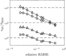
(a) Example 4.1.1: Four branch

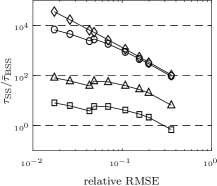
(b) Example 4.1.2: Cantilever beam

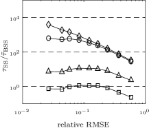
(c) Example 4.1.3: Nonlinear oscillator

Figure SM1: Efficiency of BSS with respect to subset simulation, as a function of the relative RMSE, for several values of the virtual duration $\tau_{\text{sim}}$ of a single evaluation of the function: $\tau_{\text{sim}}=1\text{ms}$ (squares), $\tau_{\text{sim}}=10\text{ms}$ (triangles), $\tau_{\text{sim}}=1\text{s}$ (circles) and $\tau_{\text{sim}}=1\text{min}$ (diamonds).

siamplain bss-paper

References

- [1] A. Arnaud, J. Bect, M. Couplet, A. Pasanisi, and E. Vazquez, Évaluation d’un risque d’inondation fluviale par planification séquentielle d’expériences, in 42èmes Journées de Statistique (JdS 2010), Marseille, France, May 24–28, 2010.
- [2] S. K. Au and J. Beck, Estimation of small failure probabilities in high dimensions by subset simulation, Probab. Eng. Mech., 16 (2001), pp. 263–277.
- [3] Y. Auffray, P. Barbillon, and J.-M. Marin, Bounding rare event probabilities in computer experiments, Comput. Statist. Data Anal., 80 (2014), pp. 153–166.
- [4] M. Balesdent, J. Morio, and J. Marzat, Kriging-based adaptive Importance Sampling algorithms for rare event estimation, Struct. Saf., 44 (2013), pp. 1–10.
- [5] M. J. Bayarri, J. O. Berger, E. S. Calder, K. Dalbey, S. Lunagomez, A. K. Patra, E. B. Pitman, E. T. Spiller, and R. L. Wolpert, Using statistical and computer models to quantify volcanic hazards, Technometrics, 51 (2009), pp. 402–413.
- [6] J. Bect, D. Ginsbourger, L. Li, V. Picheny, and E. Vazquez, Sequential design of computer experiments for the estimation of a probability of failure, Stat. Comput., 22 (2012), pp. 773–793.
- [7] J. Bect, E. Vazquez, et al., STK: a Small (Matlab/Octave) Toolbox for Kriging. Release 2.4 (to appear), 2016, http://kriging.sourceforge.net.
- [8] J.-M. Bourinet, Ferum 4.1 user’s guide. http://www.ifma.fr/FERUM, 2010.
- [9] J.-M. Bourinet, Rare-event probability estimation with adaptive support vector regression surrogates, Reliab. Eng. Syst. Saf., 150 (2016), pp. 210–221.
- [10] J.-M. Bourinet, F. Deheeger, and M. Lemaire, Assessing small failure probabilities by combined subset simulation and support vector machines, Struct. Saf., 33 (2011), pp. 343–353.
- [11] C.-E. Bréhier, L. Goudenège, and L. Tudela, Central limit theorem for adaptive multilevel splitting estimators in an idealized setting, in Monte Carlo and Quasi-Monte Carlo Methods (MCQMC 2014), R. Cools and D. Nuyens, eds., Springer, 2016.
- [12] F. Cadini, F. Santos, and E. Zio, An improved adaptive kriging-based importance technique for sampling multiple failure regions of low probability, Reliab. Eng. Syst. Saf., 131 (2014), pp. 109–117.
- [13] C. Cannamela, J. Garnier, and B. Iooss, Controlled stratification for quantile estimation, Annals of Applied Statistics, 2 (2008), pp. 1554–1580.
- [14] C. Chevalier, J. Bect, D. Ginsbourger, and I. Molchanov, Estimating and quantifying uncertainties on level sets using the Vorob’ev expectation and deviation with gaussian process models, in mODa 10 — Advances in Model-Oriented Design and Analysis, Contributions to Statistics, Springer, 2013, pp. 35–43.
- [15] C. Chevalier, J. Bect, D. Ginsbourger, E. Vazquez, V. Picheny, and Y. Richet, Fast parallel kriging-based stepwise uncertainty reduction with application to the identification of an excursion set, Technometrics, 56 (2013), pp. 455–465.
- [16] N. Chopin, A sequential particle filter method for static models, Biometrika, 89 (2002), pp. 539–552.
- [17] F. Cérou, P. Del Moral, T. Furon, and A. Guyader, Sequential Monte Carlo for rare event estimation, Stat. Comput., 22 (2012), pp. 795–808.
- [18] E. De Rocquigny, N. Devictor, S. Tarantola, et al., Determination of the risk due to personal electronic devices (PEDs) carried out on radio-navigation systems aboard aircraft, in [19], 2008, ch. 5, pp. 65–80.
- [19] E. De Rocquigny, N. Devictor, S. Tarantola, et al., Uncertainty in industrial practice, Wiley, 2008.
- [20] F. Deheeger, Couplage mécano-fiabiliste: 2SMART – Méthodologie d’apprentissage stochastique en fiabilité, PhD thesis, Université B. Pascal (Clermont-Ferrand II), 2008.
- [21] P. Del Moral, A. Doucet, and A. Jasra, Sequential Monte Carlo samplers, J. the Royal Statistical Society: Series B (Statistical Methodology), 68 (2006), pp. 411–436.
- [22] P. Del Moral, A. Doucet, and A. Jasra, An adaptive sequential Monte Carlo method for approximate Bayesian computation, Stat. Comput., 22 (2012), pp. 1009–1020.
- [23] P. Diaconis and S. Holmes, Three examples of Monte-Carlo Markov chains: at the interface between statistical computing, computer science, and statistical mechanics, vol. 72 of IMA volumes in Mathematics and its Applications, Springer, 1995, pp. 43–56.
- [24] R. Douc and O. Cappé, Comparison of resampling schemes for particle filtering, in Proceedings of the 4th International Symposium on Image and Signal Processing and Analysis (ISPA), 2005, pp. 64–69.
- [25] R. Douc and E. Moulines, Limit theorems for weighted samples with applications to sequential Monte Carlo methods, The Annals of Statistics, 36 (2008), pp. 2344–2376.
- [26] V. Dubourg, Adaptive surrogate models for reliability analysis and reliability-based design optimization, PhD thesis, Université Blaise Pascal – Clermont II, 2011.
- [27] V. Dubourg, F. Deheeger, and B. Sudret, Metamodel-based importance sampling for the simulation of rare events, in 11th International Conference on Applications of Statistics and Probability in Civil Engineering (ICASP 11), 2011.
- [28] V. Dubourg, F. Deheeger, and B. Sudret, Metamodel-based importance sampling for structural reliability analysis, Probab. Eng. Mech., 33 (2013), pp. 47–57.
- [29] V. Dubourg, B. Sudret, and J.-M. Bourinet, Reliability-based design optimization using kriging surrogates and subset simulation, Struct. Multiscip. Optim., 44 (2011), pp. 673–690.
- [30] B. Echard, N. Gayton, and M. Lemaire, AK-MCS: An active learning reliability method combining kriging and Monte Carlo simulation, Struct. Saf., 33 (2011), pp. 145–154.
- [31] B. Echard, N. Gayton, M. Lemaire, and N. Relun, A combined importance sampling and kriging reliability method for small failure probabilities with time-demanding numerical models, Reliab. Eng. Syst. Saf., 111 (2013), pp. 232–240.
- [32] P. Feliot, J. Bect, and V. E., A Bayesian approach to constrained single- and multi-objective optimization, J. Global Optim., (in press), pp. 1–37.
- [33] Free Software Foundation, GNU Lesser General Public License, version 2.1, http://www.gnu.org/licenses/old-licenses/lgpl-2.1.html.
- [34] E. Garcia, Electromagnetic compatibility uncertainty, risk, and margin management, IEEE Trans. Electromag. Compat., 52 (2010), pp. 3–10.
- [35] N. Gayton, J. M. Bourinet, and M. Lemaire, CQ2RS: a new statistical approach to the response surface method for reliability analysis, Struct. Saf., 25 (2003), pp. 99–121.
- [36] P. Glasserman, P. Heidelberger, P. Shahabuddin, and T. Zajic, Multilevel splitting for estimating rare event probabilities, Oper. Res., 47 (1999), pp. 585–600.
- [37] X. Huang, J. Chen, and H. Zhu, Assessing small failure probabilities by AK-SS: An active learning method combining kriging and subset simulation, Struct. Saf., 59 (2016), pp. 86–95.
- [38] M. E. Johnson, L. M. Moore, and D. Ylvisaker, Minimax and maximin distance designs, J. Statist. Plan. Inference, 26 (1990), pp. 131–148.
- [39] S. N. Jonkman, M. Kok, and J. K. Vrijling, Flood risk assessment in the netherlands: A case study for dike ring south holland, Risk Analysis, 28 (2008), pp. 1357–1374.
- [40] L. Li, Sequential Design of Experiments to Estimate a Probability of Failure, PhD thesis, Supélec, May 2012, https://tel.archives-ouvertes.fr/tel-00765457.
- [41] L. Li, J. Bect, and E. Vazquez, Bayesian subset simulation: a kriging-based subset simulation algorithm for the estimation of small probabilities of failure, in Proceedings of PSAM 11 & ESREL 2012, 25-29 June 2012, Helsinki, Finland., 2012.
- [42] J. S. Liu, Monte Carlo strategies in scientific computing, Springer, 2008.
- [43] J. L. Loeppky, J. Sacks, and W. J. Welch, Choosing the sample size of a computer experiment: A practical guide, Technometrics, 51 (2009), pp. 366–376.
- [44] R. E. Melchers, Structural Reliability: Analysis and Prediction. Second Edition., Wiley, 1999.
- [45] M. D. Morris and T. J. Mitchell, Exploratory designs for computational experiments, J. Statist. Plan. Inference, 43 (1995), pp. 381–402.
- [46] J. Oakley, Estimating percentiles of uncertain computer code outputs, J. Roy. Statist. Soc. Ser. C, 53 (2004), pp. 83–93.
- [47] P. P. O’Connor and A. Kleyner, Practical Reliability Engineering, Wiley, 2012.
- [48] M. Rausand and A. Hoyland, System reliability theory: models and statistical methods (second edition), Wiley, 2004.
- [49] C. P. Robert and G. Casella, Monte Carlo statistical methods, 2nd edition, Springer Verlag, 2004.
- [50] T. J. Santner, B. J. Williams, and W. Notz, The Design and Analysis of Computer Experiments, Springer Verlag, 2003.
- [51] M. L. Stein, Interpolation of Spatial Data: Some Theory for Kriging, Springer, New York, 1999.
- [52] E. Vazquez and J. Bect, A sequential Bayesian algorithm to estimate a probability of failure, in Proceedings of the 15th IFAC Symposium on System Identification, SYSID 2009, Saint-Malo France, 2009.
- [53] J. Villemonteix, E. Vazquez, and E. Walter, An informational approach to the global optimization of expensive-to-evaluate functions, J. Global Optim., 44 (2009), pp. 509–534.
- [54] P. H. Waarts, Structural reliability using finite element methods, PhD thesis, Delft University of Technology, 2000.
- [55] E. Zio and N. Pedroni, Estimation of the functional failure probability of a thermal-hydraulic passive system by subset simulation, Nuclear Eng. Design, 239 (2009), pp. 580–599.
- [56] K. M. Zuev, J. L. Beck, S.-K. Au, and L. S. Katafygiotis, Bayesian post-processor and other enhancements of subset simulation for estimating failure probabilities in high dimensions, Computers & Structures, 92–93 (2012), pp. 283–296.