Univ.-Prof. Dr. Justus Piater

Automatic Determination of Chord Roots

Abstract

Even though chord roots constitute a fundamental concept in music theory, existing models do not explain and determine them to full satisfaction. We present a new method which takes sequential context into account to resolve ambiguities and detect nonharmonic tones. We extract features from chord pairs and use a decision tree to determine chord roots. This leads to a quantitative improvement in correctness of the predicted roots in comparison to other models. All this raises the question how much harmonic and nonharmonic tones actually contribute to the perception of chord roots.

Chapter 1 Introduction

1.1 Motivation

Chord roots are of central importance in many theories of music. Therefore, it is perhaps surprising that only little research has been done in that area and many characteristics of chord roots are unknown. Several already existing theories for the prediction of chord roots have been shown to fail by Goldbach (2009). Martin Anton Schmid, a Tyrolean music theorist, formed a small research team with the goal to develop a new model to determine and explain chord roots. One of the new ideas from this group is to use the harmonic context of chords.

In this thesis we present the new basic model and an extension using the just mentioned context of chords. As far as we know, this is the first take on the topic of chord roots from a computer science perspective.

The model we describe is by no means finished nor do we claim it will work for every kind of music, but it is a first step towards a better understanding of chord roots in classical music. A long term goal of the determination of roots in musical pieces would be a harmonic analysis of chord progressions for various musical genres.

1.2 Goals

Since this project entails basic research, it was not always clear how far we would come during the course of this thesis. Nevertheless, the goals of this project were to extend the Schmid model (which we will introduce in Section 3.3) with musical context and to write a program that

• reads in existing pieces of music from some machine-readable format,

• transforms these pieces into a newly developed representation,

• determines the roots of the chords in these pieces using the new model as well as other existing models.

All these goals have been fulfilled and in addition to that 26 pieces of music (containing 2290 chords) have been annotated by hand with the “correct roots” for each chord. Using musical context we were able to determine 95.34% of the roots correctly.

Note that we focused on the development of a new algorithm and no empirical studies have been done to confirm or deny the results. This will have to be one of the next steps of our research group.

1.3 Overview

In Chapter 2 we will give a quick introduction to basic music theory, which is a prerequisite to understand the following chapters. Chapter 3 focuses on a specific part of this theory, namely the determination of chord roots. It describes several existing models and then gives an explanation of the Schmid model. Chapter 4 then introduces an extension of this model using musical context of chords, which is classified via a decision tree that we created manually, while Chapter 5 explains how we created a different decision tree automatically. Chapter 6 gives an overview of the implementation and explains how to use the program.

Chapter 2 Music Theory

This chapter will give a short but for our purposes sufficient introduction to basic aspects of music theory. For a more thorough description please refer to Ziegenrücker (2009), Grabner (1974) or Schönberg (2010). Even if you are familiar with music theory you might want to quickly read through the definitions of chords and chord roots in this chapter, because we also explain the simplifying assumptions that we used.

2.1 Basic Music Theory

2.1.1 Musical Notation

To represent a piece of music we essentially use a graph of pitch versus time. The pitch of a music note is essentially the base frequency of that note—and of course higher frequencies make higher sound. We call the horizontal lines a staff and the symbol at the beginning of the staff the clef. The vertical lines represent measures, which we will ignore in this introduction. Clefs, the symbols at the beginning, indicate what pitches the written notes have on that staff. Several staves can be written above each other, which means they are intended to be played at the same time (either by different instruments or, as in the case of the piano, by different hands). Figure 2.1 shows an example of all of these elements and more.

Figure 2.1: An example of basic musical notation.

The two staffs have different clefs at the beginning, which makes the last note in both staffs a Middle C ($C_{4}$ in Scientific pitch notation or $c^{\prime}$ in Helmholtz notation), which has a frequency of 261.626 Hertz (in equal temperament with standard pitch $A_{4}=440\;Hertz$). The second note in the second staff is a Bass C ($C_{3}$ or $c$) with exactly half the frequency of the Middle C. We say it is an octave below the $C_{4}$.

2.1.2 Notes and Pitches

The dots written on a staff are called notes. The pitches of these notes can be altered using accidentals (in addition to being determined by the clef). The only two accidentals we will use in this thesis are the sharp ($\sharp$), which raises a note by a half step and the flat ($\flat$), which lowers a note by a half step. A half step is the distance two adjacent keys on the piano keyboard, regardless of what color they may have. A step is equal to two half steps. Note that this means that it is possible to represent the same pitch in multiple ways using different notes and accidentals (e.g. $C$ and $B\sharp$). We call this enharmonic equivalence.

Note Names

The white keys on the piano keyboard are given names according to the English alphabet from $A$ to $G$—and then starting with $A$ again. This next $A$ will have exactly double the frequency as the first $A$ and we say it is an octave higher. In order to distinguish between notes with the same name, the name (or number) of the octave can added to the name of the note.

Pitch Classes

An important notion for this thesis is that of pitch classes. It is a simple mapping of note names (starting from $C$) to natural numbers between $0$ and $11$ (Forte, 1973). Octaves are ignored and the mapping is irreversible (without ambiguity). Table 2.1 shows notes and their corresponding pitch classes in integer notation with $C$ as $0$.

Note Name	Alternative Name	Pitch Class
$C$	$B\sharp$	0
$C\sharp$	$D\flat$	1
$D$		2
$D\sharp$	$E\flat$	3
$E$	$F\flat$	4
$F$	$E\sharp$	5
$F\sharp$	$G\flat$	6
$G$		7
$G\sharp$	$A\flat$	8
$A$		9
$A\sharp$	$B\flat$	10
$B$	$C\flat$	11

Table 2.1: Note names (without octaves) and their corresponding pitch classes.

2.1.3 Rhythm

Notes of course do not only have a pitch, but also a length, which is what gives a piece its rhythm. A special notation for “a time of silence” also exists and is called a rest. Rests can also have different lengths. Note that these lengths do not say anything about the absolute time a note should be played (or nothing should be played in the case of the rest), but rather it notates the time it should take in relation to the other notes. Figure 2.2 shows an example of both notes and rests with common lengths.

Figure 2.2: Common lengths of notes and rests.

The first note is a whole note and each following note has half the length of the

previous one. The same applies to the rests in the second staff.

2.1.4 Intervals

The last important notion in this section is that of the interval, which describes the distance between two pitches. To calculate this distance, simply count the number of half steps it takes to reach the top note from the bottom one. These distances are then again given names. Figure 2.3 shows some examples of intervals that will be needed later on.

Figure 2.3: The three intervals Minor third, Perfect fifth and Perfect octave.

2.2 Chords

We decided to take the definition from Schmid (2014, personal communication):

Definition 1 (Chord).

A chord is a combination of two or more tones with different pitch classes sounding simultaneously or immediately in succession.

Schmid also claims that “The connection between between successive tones can sometimes only be determined in the harmonic context and sometimes not at all.”

With this definition we do not distinguish between intervals (i.e. chords with only two notes) and chords with three or more notes. In addition to that we make another simplification: We do not view arpeggios, broken chords and so forth (i.e. the tones sounding immediately in succession) as chords, because simply not enough research has been done in this area. It is for example not clear how fast (in absolute time) a broken chord has to be played to be perceived as a chord (with a root). It will probably be necessary to revise this definition after further research. Figure 2.4 shows several examples of note combinations. Only the third and fourth example are chords in the sense of our simplified definition.

(a) A single note

(b) A broken $Cmaj$ chord

(c) An interval

(d) $A\flat{}maj7$ chord

Figure 2.4: A single note and three note combinations, of which we only consider (c) and (d) as “chords”.

Definition 2 (Chord Progression).

A chord progression is a sequence of two or more chords.

A chord progression usually gives a piece of music its harmonic movement and is sometimes even called harmonic progression (Schönberg, 1969). It is the main reason we want to determine chord roots, which we will define shortly.

2.2.1 Nonharmonic Tones

Definition 3 (Nonharmonic Tone).

A nonharmonic tone (also called nonchord tone) is a note in a chord which does not fit into the established harmonic framework. A chord may contain zero, one or more nonharmonic tones.

Nonharmonic tones are almost always dissonant (Schmid, 2015, personal communication), which means the chord they are played in will sound “harsh” or “unpleasant”, in contrast to a chord containing only consonant tones, which will sound “sweet” or “pleasant”. Note that, as Hindemith (1942) stated, the two concepts of consonance and dissonance “have never been completely explained, and for a thousand years the definitions have varied”.

Music theorists distinguish between many different forms of nonharmonic tones, which are described in most introductions to music theory. If we know the root of a chord, its nonchord tones can in most cases easily be determined, although we did not focus on that in this thesis. Figure 2.5 shows an example of a suspension—a common type of nonharmonic tones in the Bach corpus.

Figure 2.5: Example of a suspension ($G$) in the second measure.

2.3 Chord Roots

We used the following working definition:

Definition 4 (Chord Root).

The root of a chord is its perceptional reference note, on which the chord progression of a piece can be analysed. A chord might have more than one correct root. Sometimes the root(s) of a chord cannot be determined.

Figure 2.6 shows an example of a simple chord progression with the roots of the chords and roman numerals written below each chord. $G$ is 4 steps above $C$ and $A$ is 4 steps above $D$, which means the chord progressions are actually the same: “four steps down”.

Figure 2.6: An example of the same chord progression created by different chords. (Schmid, 2014)

Chapter 3 Determination of Chord Roots

In this chapter we describe how chords can be created by stacking thirds and how several existing models for the determination of roots analyse chords. Then Schmid’s new model is introduced. Finally, it is shown how chords are extracted from note sequences and an analysis example of such a sequence is given.

3.1 Constructing Chords

The classical way to generate a chord would be to take a note as root (e.g. $C$) and stack a third and a fifth above it. For a $Cmaj$ chord you would take a Major third ($E$) and a Perfect fifth ($G$) to get $C-E-G$. For $Cm$ the Minor third is needed first and then again the Perfect fifth ($C-E\flat-G$). Note that in both cases the highest note is a third above the second highest note: A Minor third in the first and a Major third in the second chord. If we stack another third above each chord we get a $Cmaj7$ ($C-E-G-B$) or $Cm7$ ($C-E\flat-G-B\flat$) chord. This method of generating chords goes back to Rameau (1971).

3.2 Existing Models

As mentioned in the beginning, Goldbach (2009) showed that all existing models fall short of correctly determining chord roots in many cases. Nevertheless, they are quite interesting and useful for comparisons for the model of Schmid and we will have a look at them in the remainder of this section. We will do a detailed analysis of the chord $E_{4}-G_{4}-C_{5}$ by each model after describing it. These models were also implemented in our program.

3.2.1 Stacking Thirds

This describes most well known method of finding the root of a chord (actually it is the method that is taught in most music classes to determine the name of a chord, which does not necessarily coincide with its perceptual root). We basically try to reverse the process of generating a chord that we just introduced in Section 3.1:

Ignore octaves and stack as many notes as possible with distance of a third above each other. The lowest note will be the root. Note that this addresses primarily how a chord is notated in contrast to how a chord sounds, which is what the following models will do. Figure 3.1 shows an example of this method.

Figure 3.1: Analysis of a $Cmaj$ chord in its first inversion by stacking thirds.

$E$ has one third above it, $G$ has zero thirds directly above. $C$ can have both the other notes stacked above it and we determine it as the root.

3.2.2 Ernst Terhardt

Terhardt (1982) based his model on the first ten subharmonic partials of each note in a chord:

Definition 5 (Subharmonic Partial).

The n’th subharmonic partial P of a note $X$ with frequency $f_{X}$ is a tone with frequency $f_{P}=f_{X}/n\;$ with $\;n\in\mathbb{N}\setminus\{0\}$.

Ignoring octaves, each note in a chord has five different notes in its first ten subharmonic partials (which include the note itself). These partials correspond (approximately) to the following intervals: Perfect unison, Perfect fifth below, Major third below, Major second above and Major second below. After having determined the subharmonic partials for each note in the chord, the frequency of each note is counted. Each note that appears $d$ times in the subharmonic partials of the notes in the chord is determined as a “root of degree $d$” of the chord.

The note with the highest degree (which is not necessarily unique) is then determined as “the” root of the chord, although Terhardt described qualitative features which can also alter the root of a chord (e.g. partial $n$ is “more important” than partial $n+1$). Since these features are not well defined, we will not described them in detail here (and our implementation ignores them). Table 3.1 shows how, again, $C$ is determined as the root of the chord $E_{4}-G_{4}-C_{5}$.

Perfect unison	$E$	$G$	$C$
Perfect fifth below	$A$	$C$	$F$
Major third below	$C$	$E\flat$	$A\flat$
Major second above	$F\sharp$	$A$	$D$
Major second below	$D$	$F$	$B$
2nd degree roots		$D,\;F,\;A$
3rd degree root		$C$

Table 3.1: Analysis of a $Cmaj$ chord in its first inversion using Terhardt’s model.

3.2.3 Richard Parncutt

Parncutt (1997) based his model on Terhardt’s, but extended it in the following ways:

He states that the partials are of different importance and assigns them different weights. To strengthen the bass as possible root, he adds an additional arbitrary weight to the bass note of the chord. Finally he makes a distinction between different tonalities (major or minor) and assigns each interval for each tonality a different additional weight. The note with highest final weight is determined as the root of the chord. In Table 3.2 we can see that in this model both $C$ and $E$ could be roots of the chord.

	$C$	$C\sharp$	$D$	$D\sharp$	$E$	$F$	$F\sharp$	$G$	$G\sharp$	$A$	$A\sharp$	$B$
Perfect unison	10				10			10
Perfect fifth below	5					5				5
Major third below	3			3					3
Major second below			2				2			2
Major second above			1			1					1
Tonality (Cmajor)	33		10	1	17	15	2	24	1	11		5
Bass					20
Overall Weights	51		13	4	47	21	4	34	4	18	1	5

Table 3.2: Analysis of a $Cmaj$ chord in its first inversion using Parncutt’s model.

The large weight that is given to the bass note ($E$) means this is tight race between $C$ and $E$. Parncutt states that values differing by less than 5 should be regarded as the same, which actually makes it so that both notes can be seen as roots.

3.3 A New Model

3.3.1 Assumptions and Representation

For the development of the model we made several assumptions, which will be described here on the representation of the example-chord $C_{4}-E_{4}-G_{4}-B\sharp_{5}$:

Enharmonic Equivalence

We ignore enharmonic equivalence as it is (in the equal temperament) just a difference in notation and does not contribute anything to the hearing. We simply choose one of the notations.
$C_{4}-E_{4}-G_{4}-B\sharp_{5}\quad\rightarrow\quad C_{4}-E_{4}-G_{4}-C_{6}$

Octaves

We hypothesize that the absolute height of a note is not relevant for the determination of chord roots and can therefor be ignored.
$C_{4}-E_{4}-G_{4}-C_{5}\quad\rightarrow\quad C-E-G-C$

Duplications

We decided to ignore duplications of chords, because we assume that for the perception of the chord it does not matter how many instruments play a certain note.
$C-E-G-C\quad\rightarrow\quad C-E-G$

Pitch Names

The pitches of a chord only have meaning in relation to each other. This means that for example $C-E-G$ and $D-F\sharp-A$ will have the same relative root: If we map them to their respective pitch classes and normalize them so that the first pitch class is $0$, they will both have root “0”. (To get the name of the root, this mapping has to be inverted.)
$C-E-G\quad\rightarrow\quad 0-4-7\quad$ and also $\quad D-F\sharp-A\quad\rightarrow\quad 0-4-7$

Note that all of these assumptions are also made by the other described models.

3.3.2 Definition

Schmid leans heavily on the method of stacking thirds and his model works as follows:

For each note in a chord, stack the other notes on top of it so that the distance between this note and the highest note is minimal, but the distance between each two notes is at least 3 (Minor third). The notes with the lowest minimal distance are the roots of the chords.

The distance 3 is used, because it represents the smallest interval (except the unison) that human hearing still perceives as consonant. Smaller intervals are usually rated as dissonant by test persons (Roederer, 2000).

Example

We will show how this works on the following chord: $G-B-D-F\sharp-G$

1. Transform the chord into our developed representation:
   $G-B-D-F\sharp-G\quad\rightarrow\quad 0-4-7-11$

2. For each note, stack the others above it with minimal distance 3 and measure the distances to the highest note:
   
   Assumed Root Stacked with Minimal Distance (Normalized Pitch Classes) Distance 0 ($G$) $0\;(G)-4\;(B)-7\;(D)-11\;(F\sharp)$ 11 4 ($B$) $0\;(B)-3\;(D)-8\;(G)-17\;(F\sharp)$ 17 7 ($D$) $0\;(D)-5\;(G)-9\;(B)-16\;(F\sharp)$ 16 11 ($F\sharp$) $0\;(F\sharp)-5\;(B)-8\;(D)-13\;(G)$ 13

3. We determine $G$ as the root of the chord, because its distance is 11 which is smaller than 13, 16 and 17.

Ambiguous Examples

These next two examples show that this determination is not always unambiguous.

• First consider the chord $C-G\sharp-A\sharp$: According to Schmid its root can either be the $G\sharp$ or the $A\sharp$, because they both have distance 14.
  
  Assumed Root Stacked with Minimal Distance (Normalized Pitch Classes) Distance 0 ($C$) $0\;(C)-10\;(A\sharp)-20\;(G\sharp)$ 20 8 ($G\sharp$) $0\;(G\sharp)-4\;(C)-14\;(A\sharp)$ 14 10 ($A\sharp$) $0\;(A\sharp)-10\;(G\sharp)-14\;(C)$ 14

• Now consider the chord $E-G-A\sharp-C\sharp$: For each note the minimal distance is the same (9), because the pitch classes are always $0-3-6-9$, regardless of the lowest note! This is just one of several possible cyclic chords, for which nothing can be determined.
  
  Assumed Root Stacked with Minimal Distance (Normalized Pitch Classes) Distance 0 ($E$) $0\;(E)-3\;(G)-6\;(A\sharp)-9\;(C\sharp)$ 9 3 ($G$) $0\;(G)-3\;(A\sharp)-6\;(C\sharp)-9\;(E)$ 9 6 ($A\sharp$) $0\;(A\sharp)-3\;(C\sharp)-6\;(E)-9\;(G)$ 9 9 ($C\sharp$) $0\;(C\sharp)-3\;(E)-6\;(G)-9\;(A\sharp)$ 9

3.3.3 Interval Order

To be able to choose an unambiguous root from two or more ambiguous roots, Schmid proposes to use an interval order, in which the intervals are ordered by “importance”. The intervals to the previous and following chord (i.e. the distances between the pitch classes of the roots) have to be determined and rated. Figure 3.2 displays two possible interval orders and Figure 3.3 shows them used in an example.

$$(a)\quad 0\;>\;7\;>\;5\;>\;4\;>\;8\;>\;3\;>\;9\;>\;2\;>\;10\;>\;1\;>\;11\;>\;6$$

$$(b)\quad 0\;>\;7\;=\;5\;>\;4\;=\;8\;>\;3\;=\;9\;>\;2\;=\;10\;>\;1\;=\;11\;>\;6$$

Figure 3.2: Two possible interval orders for the determination of unambiguous roots.

The numbers represent the number of semitones between the two compared pitch classes. Both orders rate the Perfect unison (or Perfect octave) the highest. The first order classifies the Perfect fifth above higher than the Perfect fifth below, while the second order values them with equal importance. Then this continues with the remaining intervals.

Figure 3.3: Interval order examples.

The first chord is a simple $Cmaj$ chord ($C-E-G-C$) with root $C$, while the root of the second chord ($C-E-G-D$) is ambiguous ($C$ or $D$). Since the interval between $C$ (root of the first chord) and $C$ (first possible root of the second chord) is rated higher in the interval orders than the interval between $C$ and $D$ (Perfect unison (0) $>$ Major second (2)), the $C$ is chosen as the root for the second chord.

3.4 Chordification

In order to determine the roots of chords in a pieces of music, we first need to “combine” the chords (from different voices). Our definition of chords makes this easy: Whenever one or more notes start or stop sounding, a new chord is created (regardless of the voice the note appears in).

Figure 3.4 shows an example of this chordification in two steps: First all the notes get assigned list of numbers indicating in which chords they will sound in and then for each number a new chord is created.

$\mathrel{\scalebox{2.8}[2.5]{$\downarrow$}}$

$\mathrel{\scalebox{2.8}[2.5]{$\downarrow$}}$

Figure 3.4: Chordification of a note sequence in two steps.

3.5 Example Analysis

Now that we know how to combine chords and determine roots, we can look look at a complete example of an analysis of (the beginning of) a real-world musical piece in Figure 3.5.

	1	2	3	4	5	6	7	8	9	10
Stacking Thirds	$G$	$A$	$G$	$G$	$G$	$G$	$C$	$C$	$C$	$G$
Terhardt	$C$	$C$, $D$, $F$, $G$	$C$	$C$, $B\flat$	$G$	$G$	$F$	$C$, $F$	$C$	$G$
Parncutt	$G$	$G$	$G$	$G$	$G$	$G$	$E\flat$	$D$	$C$, $G$	$G$
Schmid	$G$	$A$	$G$	$G$	$G$	$G$	$C$	$D$	$D$	$G$
Correct Roots	$G$	$G$	$G$	$G$	$G$	$G$	$C$	$C$	$G$	$G$

Figure 3.5: An analysis of a short chord sequence by different models.

The ensemble staff above shows the beginning of BWV 14.5 (in G minor) with numbered notes (so the reader can see the original score, but also easily construct the chords). The table below depicts the root(s) each model determined per chord. The correct roots were annotated by hand (This represents my own subjective intuition of what should be the “correct root” when taking nonharmonic tones into account.) We can see that all models predict some of the roots differently. Stacking thirds actually seems to come the closest to my predicted “correct roots”.

Chapter 4 Musical Context

A potential problem of Schmid’s basic model is that in the model no distinction is made between nonharmonic and harmonic tones for the determination of roots. We will now introduce a new model called Context, which extends the Schmid model. It will try to predict nonharmonic tones through the musical context and then ignore them for the determination of roots. First, chord groups are formed out of chord sequences and then it is shown how chords influence each other within their groups. Note that we are only considering the Bach corpus (tonal music) in this thesis.

4.1 Chord Groups

First we introduce a new concept we call chord groups, which are simply sequences of chords:

In the beginning we put each chord in its own group and then, whenever two consecutive chords share at least one note (i.e. the note sounds in both chords), we merge the two groups in which they are contained. Note that this shared note actually needs to be the same note and not two different notes with equal pitch. Figure 4.1 shows an example of this being done during the chordification we saw in Figure 3.4. The black double bars delimit the groups.

Within these groups it is now possible that neighboring chords influence each other during the determination of roots: Chords may contain nonharmonic tones, which gain meaning in combination with the previous or following chords. It is obvious that with this definition, chords in chord groups of size 1 do not change. From here on forth we will mean “chord groups of size 2 or bigger” when we talk about chord groups.

$\mathrel{\scalebox{2.8}[2.5]{$\downarrow$}}$

Figure 4.1: Creation of four different chord groups of different sizes.

4.2 Features

As a start we will look at chord groups of size 2, which we will call chord pairs. In order to be able to begin analysing them, we first need to extract some features, which we will define in this section.

Determined Root

To each chord $c$ we assign a set $R(c)$ in which all its possible roots (or rather the pitch classes of the roots) are contained. These roots are determined by the Schmid model.

Unique Root

A chord can have a unique root or it can have multiple roots. If a chord $c$ has a unique root we say $U(c)$ is true:

$$U(c)\quad\iff\quad size(R(c))=1$$

Stack of Thirds

As described earlier, the new model gives a lot of weight to minimal distances, but completely ignores maximal distances. Figure 4.2 shows how these might actually be useful:

(a) $Cmaj$ with suspension

(b) The first chord stacked on top of $D$

Figure 4.2: An example where maximal distances are useful.

The first chord in (a) is $C-E-G-D$ which contains the nonchord tone $D$, the second chord in (a) is a normal $Cmaj$ chord ($C-E-G-C$). The root of the second chord is $C$. For the root of the first chord both $C$ and $D$ are predicted as possible roots, because they both a minimal distance of 14, even though the $C$ might make more sense if we disregard at $D$ as nonharmonic tone.

To combat this we introduce a new feature $N(c)$ for chord $c$, which will “limit” the maximal distance between the root (lowest note) and highest note. It is defined as

$$N(c)\quad\iff\quad d(c)\;\;\leq\;\;4\times(P(c)-1)$$

where $d(c)$ is the mentioned distance and $P(c)$ the number of different pitch classes in the chord. This basically means that we restrict the distance between each two notes to 4 (Major third), which again leans heavily on the idea of stacking thirds. If the distance is greater, this feature gives a first hint that we should look at this chord more closely as it might for example contain nonharmonic tones.

Containment and Difference

A chord $c_{A}$ (or set of roots $R(c_{A})$) is contained in $c_{B}$ if all of the pitch classes of the notes contained in $c_{A}$ are also contained in the pitch classes of the notes of $c_{B}$. If $c_{A}$ is contained in $c_{B}$ we write $c_{A}\subseteq c_{B}$. We say that two chords are equal if they are both contained in each other. (E.g. $C_{4}-C_{3}-C_{5}-E_{4}-G_{3}-G_{2}\;\;=\;\;C_{4}-E_{4}-G_{4}$)

Similarly, the difference of the chords ($c_{A}-c_{B}$) is defined as the set of all notes the pitch classes of which are contained in $c_{A}$ but not in $c_{B}$.

Partial Sub-Chord

We say chord $c_{A}$ is a partial sub-chord of chord $c_{B}$ if one of the following conditions holds:

• $c_{A}$ is contained in $c_{B}$:

  $$c_{A}\subseteq c_{B}$$

• None of the roots of $c_{B}$ are contained in $c_{A}$ and the unique root of $c_{A}$ is contained in $c_{B}$:
  

  $$c_{A}-R(c_{B})=c_{A}\quad\land\quad R(c_{A})\subseteq c_{B}\quad\land\quad U(c_{A})$$

We write $c_{A}\unlhd c_{B}$ to express that $c_{A}$ is a partial sub-chord of $c_{B}$. Figure 4.3 depicts the motivation behind this feature.

(a) First chord is fully contained

(b) Second chord contains nonharmonic tone

(c) First chord contains nonharmonic tone

(d) First chord might contain two nonharmonic tones

Figure 4.3: Examples of partial sub-chords.

(a)

The first chord ($D-F\sharp-A-D$, predicted root $D$) is fully contained in the second chord ($D-F\sharp-A-E$, predicted roots $D$ or $E$) and is therefore a partial sub-chord. If we look at the $E$ as a nonharmonic tone, it would probably not make sense to set it as the root of the chord. The partial sub-chord is supposed to help with this decision as it tells us that the root of the first chord might be more important and that we will set the root of the second chord to $D$.

(b)

The second condition comes into play: The root of the first chord ($E$) is contained in the second chord, but the root of the second chord ($C\sharp$) is not contained in the first chord. We will assume $C\sharp$ is a nonchord tone and set the root for the second chord to $E$.

(c)

Here the reverse of (b) happens: We will assume $F$ (the root of the first chord) is a nonharmonic tone and set the root to $A$ (the root of the second chord) instead.

(d)

The first chord is $G-D-A-C$ with determined root $A$ and the second chord is $G-D-G-B$ with determined root $G$. We will take the (potentially controversial) step of assuming both $A$ and $C$ as nonchord tones and setting the root of the first chord to $G$. For pieces outside of the Bach corpus this might not work that well and additional restrictions will have to be developed. Note that the $H$-feature prevents a chord from having more nonharmonic tones than harmonic tones.

(a) Two separate chords

(b) Bass note changes

(c) Highest note changes

Figure 4.4: Differences in changing tones in a chord pair.

In (a) we see the two separate chords $Cmaj7$ and $Emaj$ (which unlike in (b) and (c) do not form a chord pair). With our current representation we can not distinguish between the two progressions in (b) and (c). In (b) the bass note changes, which means the roots are probably $C$ and $E$, while in (c) the highest note changes which makes it more likely that the root is $E$ for both chords (Schmid, 2015, personal communication).

Number of Changing Notes

We count the number of notes in chord $c$ that still sound from the previous chord (which by definition is in the same chord group) and the number of notes that only start sounding in the current chord. We say $H(c)$ holds, if there are more “new” notes (that just started sounding) than “old” ones (which already sounded in the previous chord). In short, $H(c)$ is true if “more than half the notes changed from the previous chord”. Note that most chords in our considered Bach corpus consist of three or four different notes which reduces the decision to “Is at most a single note still sounding from the previous chord?”.

This again works for most of the Bach corpus, but it also reveals a potential problem of our representation of chords, as can be seen in Figure 4.4, because we do not distinguish between voices and ignore absolute pitches.

4.3 Decision Tree for Chord Pairs

Having determined useful features of our chord pairs, we can now start building a decision tree. The input of the tree will be the arbitrary chord pair ($X$, $Y$), complete with all the features that were just described, and the output will be the two new (sets of) roots $R_{X}$ and $R_{Y}$. The following sections will explain all the decisions that are made in the tree and give examples of correctly determined roots for chord pairs made possible by these decisions.

The whole tree in the form of a graph is displayed in Figure 4.5.

Figure 4.5: The decision tree for an arbitrary chord pair $(X,Y)$.

The solid lines represent “condition holds”, the dotted lines represent “condition does not hold”.

Note that there are three different endpoints where we do not change anything: If we reach the “ignore”-endpoint on the left we are confident that ignoring the context is okay. If we reach the “insufficient training data”-node at the top right corner, we do not know enough to make a sensible decision so we ignore it due to the lack of further meaningful features and the fact that very few samples from our corpus reach this point. At the bottom “no more features”-node we know that most features do not hold, which again forces us to ignore the pair. The following sections will explain the decisions that lead to these node more in-depth.

4.3.1 Same Unique Root

We start by filtering out all the pairs that already have the same unique root ($R(X)=R(Y)\;\;\land\;\;U(X)$). This is done because we assume that the Schmid model is (in most cases) able to determine the correct roots for isolated chords and that it is very likely for chords in their chord pair to have the same root. The two most prominent cases in which this rule is helpful are

• The chords are equal

• One chord is contained in the other one, which contains an additional (often harmonic) tone (e.g. the seventh of a triad)

These pairs are simply ignored and their determined roots are not changed. Figure 4.6 shows two chord pairs to which this condition applies.

(a) Equal chords

(b) Second chord contains $7th$

Figure 4.6: Chord pairs where both chords have the same unique root.

4.3.2 $X$ is Stack of Thirds

As the section title suggests, we now decide whether or not $X$ is a stack of thirds. If it is not, it might contain at least one nonharmonic tone. If $X$ is a stack of thirds, there is a good chance that we already determined its root correctly, but in both cases we need some more information.

• If $N(X)$, we calculate if more than half the notes change from $X$ to $Y$

  • $H(Y)\rightarrow$ continues immediately in Section 4.3.3

  • $\lnot H(Y)\rightarrow$ continues in Section 4.3.4

• If $\lnot N(X)$, we will make the next decision in Section 4.3.5

4.3.3 More Than Half the Notes Change

$H(Y)$ essentially tells us that $X$ and $Y$ are only loosely connected and most of their notes do not influence each others root.

In this branch we have only one last decision to make: Is $Y$ is also a stack of thirds? If it is, we again leave both roots unchanged (although they could be different now). If $\lnot N(Y)$ we have to do more work, because we know that $Y$ probably contains nonharmonic tones which still sound from $X$. The solution is to remove from Y all those notes of X that still sound (less than half the notes) and determine the roots of this subset of $Y$ without context. Figure 4.7 shows examples of this branch.

(a) BWV 244.15

(b) BWV 13.6

Figure 4.7: Chord pairs where more than half the note change.

(a)

This depicts the first case where $N(Y)$ holds: The chord with number 4 is $C\sharp-C\sharp-E-A$ and the next chord is $D\sharp-B-F\sharp-A$ (only $A$ keeps sounding). Both are stacks of thirds and the roots, $A$ and $B$ respectively, are determined without context. The chord pair 8–9 also falls in this category

(b)

We see that both chord pairs 42–43 and 44–45 have $\lnot N(Y)$. The $F$ is removed from both chord 43 and chord 45, which leaves us with the root $G$ in both cases. Chords 42 and 44 both have root $F$.

4.3.4 Not More Than Half the Notes Change

If only less than half or half the notes change, we know that the two chords are more closely related and it is probable that they have the same root. We now check if one of the partial sub-chord conditions holds:

• If $X\unlhd Y$, we set the root of $Y$ to that of $X$

• If $\lnot(X\unlhd Y)$, we check the reverse:

  • If $Y\unlhd X$, we set the root of $X$ to that of $Y$

  • If $\lnot(Y\unlhd X)$, but $U(X)$ and $R(X)\subseteq Y$, we again set the root of $Y$ to that of $X$

  • Otherwise we leave both roots unchanged

Figure 4.8 shows example of these branches.

(a) $X\unlhd Y$

(b) $Y\unlhd X$

(c) $U(X)\land R(C)\subseteq Y$

(d) Leave unchanged

Figure 4.8: Chord pairs where $N(X)$ and not more than half the notes change.

(a)

$X$ is contained in $Y$ and therefore also a partial sub-chord of $Y$. We set the root of $Y$ to $A$. A similar example was already shown in Figure 4.3(a).

(b)

The predicted root of $Y$ ($D-D-F-B$) is $B$, which is not contained in chord $X$ ($D-D-F-A$), but the root of $X$ ($D$) is contained in $Y$, so the root of $Y$ is set to $D$. Again, we have already seen a similar example in Figure 4.3(b).

(c)

Both chords are not partial sub-chords of each other. The predicted root for $X$ is $B\flat$, which is unique and contained in $Y$, while $Y$ has the predicted root $F$, which is not contained in $X$. We determine the root of $Y$ as $B\flat$.

(d)

The predicted root for $X$ ($C-A-A-C$) is $A$, while the predicted root for $Y$ ($C-D-B\flat-C$) is ambiguous: either $C$ or $B\flat$. Both chords are not partial sub-chords of each other and the root of $X$ is not contained in $Y$, so we leave the roots unchanged. This means we were unable to determine an unambiguous root for chord $Y$.

4.3.5 $Y$ is Stack of Thirds

The branch in which $N(Y)$ holds will almost mirror the decisions in Section 4.3.2, with the exception that we already know $\lnot N(X)$. Again we first check if more than half the notes change and then if one of the partial sub-chord conditions holds.

• If $H(Y)$, we assume the notes that still sound in $Y$ only belong to $Y$ and remove them from $X$ to determine the roots of this subset of $X$ without context. Figure 4.9 shows examples of chord pairs where this holds.

• If $\lnot H(Y)$, we continue in Section 4.3.6.

(a) Root of the first chord changes

(b) Root does not change

Figure 4.9: Chord pairs where more than half the notes change.

(a)

The first chord is $G-B\flat-D-C$ with predicted roots $C$ or $B\flat$ and is not a stack of thirds. The second chord is $A-C-E-C$ with root $A$ and is a stack of thirds. As we can see, only a single note still sounds in the second chord and we therefore remove that note from the first chord. With $sub(X)=G-B\flat-D$ we get the unambiguous root $G$ for $X$.

(b)

Sometimes the root of a chord does not change when we take out a note. We remove the highest $F\sharp$ from the first chord, but there is still the $F\sharp$ from the bass and its root remains $F\sharp$. The root of the second chord also remains $G\sharp$.

4.3.6 Partial Sub-Chords Mirrored

• If $Y\unlhd X$, we set the root of $X$ to that of $Y$

• If $\lnot(Y\unlhd X)$, we again check the reverse:

  • If $X\unlhd Y$, we set the root of $Y$ to that of $X$

  • If $\lnot(X\unlhd Y)$, but $U(Y)$ and $R(Y)\subseteq X$, we again set the root of $X$ to that of $Y$

  • Otherwise we leave both roots unchanged

4.3.7 No Stack of Thirds

This is where some special chords appear. There are simply not enough examples of that in the Bach corpus we used to come up with meaningful rules beyond just accepting the roots that were determined without context. Two examples are displayed in Figure 4.10.

(a) Roots are predicted unambigously

(b) Ambiguous Roots

Figure 4.10: Chord pairs without a stack of thirds.

(a)

For the first chord the $E$ is predicted as root, and for the second chord the $F$. In both cases we have a rather dissonant interval in the bass voice.

(b)

The root determination of the first chord is ambiguous: either $G$ or $A$. For the second chord we determine $C$ as the root (which means we assume that the third is missing from the chord, but fifth and seventh are present).

4.3.8 Possible Outcomes

To summarize, we have five possible outcomes for the arbitrary chord pair ($X$, $Y$):

• Do not change the previously determined roots for either chord

• Set the root of $X$ to that of $Y$

• Set the root of $Y$ to that of $X$

• Change the root of $X$ by removing some notes from $X$ and determining the root again without context

• Change the root of $Y$ by removing some notes from $Y$ and determining the root again without context

4.4 Larger Chord Groups

For larger groups (i.e. groups with size larger than 2) we only use a single rule as a first approach.

4.4.1 Reduction to Pairs

We split the group into pairs. All the chords in the group except the first and the last one will be part of exactly two groups (once as the first chord and once as the second chord). Then we run all the pairs through the decision tree and check if for each chord the results are the same in its two groups. Whenever the determined roots for a chord are the same, we set the root of this chord to this determined root. If the roots are different, we keep the root that was computed without any context. Figure 4.11 shows how this is done on chord groups of length 3 and 4.

(a) BWV 429

(b) Group of length 3 (2 pairs)

(c) BWV 6.6

Figure 4.11: A reduction of a large chord group to pairs.

(a)

The first and third chord consist of exactly the same notes, while the second chord contains the nonharmonic tone $F\sharp$ (which is also determined as the root). This is spotted and the root of the second chord is set to $A$, the root of the other two chords (c.f. Section 4.3.4).

(b)

The second group is reduced to the two pairs (the asterisks mark notes that did not change):

• $C-E\flat-G-C$ (root $C$) and $F-A-F-C^{*}$ (root $F$)
  We leave both roots unchanged (c.f. Section 4.3.3).

• $F-A-F-C^{*}$ (root $F$) and $F^{*}-A^{*}-E\flat-C^{*}$ (root $F$ or $E\flat$)
  We determine $F$ as the root of the second chord in this pair (c.f. Section 4.3.4).

Now we check if the predicted roots for the same chord in different pairs are equal. In this case we just have to check the second chord which has root $F$ in both pairs and we determine the roots $C$, $F$ and $F$ for this group.

(c)

Here we have 3 pairs:

• $F-E\flat-A-C$ (root $F$) and $F^{*}-D-B\flat-B\flat$ (root $B\flat$)
  We do not change either root (c.f. Section 4.3.3).

• $F^{*}-D-B\flat-B\flat$ (root $B\flat$) and $F-E\flat-B\flat^{*}-C$ (root $C$)
  We change the root of the second chord to $F$ (c.f. Section 4.3.3).

• $F-E\flat-B\flat^{*}-C$ (root $C$) and $F^{*}-C-A-C^{*}$ (root $F$)
  We change the root of the first chord to $F$ (c.f. Section 4.3.6).

Again we check if the changed roots are the same, which is the case for the single changed root of chord 3 as it is set to $F$ in both pairs. We predict the roots $F$, $B\flat$, $F$ and $F$ for this chord group.

Chapter 5 Generation of a Decision Tree

The biggest challenge in creating a classifier for chord pairs was to find meaningful features. The decision tree that was introduced in the previous chapter was then created by hand. We also generated such a tree automatically, which will be described in this chapter.

5.1 Training

For the creation of the decision tree we used the Python library scikit-learn (Pedregosa et al., 2011). Gini impurity was used as the error measure. To prevent overfitting, we set the parameter “min_samples_leaf=10” so that it would stop splitting if less than 10 sample would be in the split branches. The training data consisted of 613 chord pairs $(X,Y)$ of which we manually annotated the following 8 features (with either “true” or “false”):

• $N(X)$

• $N(Y)$

• $X\unlhd Y$

• $Y\unlhd X$

• $R(X)=R(Y)\;\land\;U(X)$

• $H(Y)$

• $U(X)\land R(X)\subseteq Y$

• $U(Y)\land R(Y)\subseteq X$

In addition to that each pair was annotated with a class, which denoted the suspected outcome of its analysis (which were already listed in Section 4.3.8):

• Do not change the previously determined roots for either chord

• Set the root of $X$ to that of $Y$

• Set the root of $Y$ to that of $X$

• Change the root of $X$ by removing some notes from $X$ and determining the root again without context

• Change the root of $Y$ by removing some notes from $Y$ and determining the root again without context

As only restriction we chose to stop splitting when a split would create a node with less than 10 training samples to avoid over-fitting.

5.2 Outcome

The generated tree is displayed in Figure 5.1.

Figure 5.1: Automatically created decision tree for an arbitrary chord pair $(X,Y)$.

The solid lines represent “condition holds”, the dotted lines represent “condition does not hold”.

Note that the tree only uses 4 of the 8 possible features.

The tree yielded a 96.23% accuracy on the test-data (consisting of 106 samples, which were taken out of the original data before creating the tree). When running on our corpus of 26 manually annotated musical pieces from Johann Sebastian Bach, the generated tree was able to determine 85.01% of the roots correctly, while the manually created tree achieves an accuracy of 95.34%. The tree we created by hand also makes use of more features and we think that it makes a bit more sense from a music theoretical standpoint (E.g. for the outcome $R(Y)\Rightarrow R(X)$ it is actually important that $\lnot N(X)$, which is checked in our manual tree, but not in the generated tree.). The automatic tree also does not ignore data, when not enough features hold. Our program includes the code for both trees, but uses the manually generated one by default.

Chapter 6 Implementation

In this chapter we give a short overview of the capabilities of our program and the technologies we used. Then we give a brief introduction on how to use the program via both command line and graphical user interface.

In general, readability and extensibility were favored over efficiency in our implementation (e.g. roots of some of the models could be calculated more quickly, but the ideas of the models would not be obvious anymore and the speed gain would probably be imperceptible).

6.1 Capabilities

Our program is able to

• Read in musical pieces (either a single piece or all pieces in a certain directory) encoded in various file formats.

• Analyse these pieces using the following models:

  • Stacking Thirds (from the music21 library; see Section 6.2)

  • Terhardt

  • Parncutt

  • Schmid (with and without interval order)

  • Context

• Output the following files:

  • HTML file containing the analysis for each chord from the analysed musical piece

  • MusicXML file containing the original piece with the number(s) of each chord annotated in the ‘lyrics’

  • Textfiles for each model containing the determined roots for the chords (one per line)

6.2 Used Technologies

The main programming language that was used is Python 3. Our code depends heavily on the music21–library for things such as parsing the input files or writing out the numbered MusicXML files. The GUI was created with PyQT5. The HTML files include some JavaScript which uses the libraries jQuery and VexFlow (to display staves and notes). The CSS framework Bootstrap was used to improve formatting and make the tables look nice.

6.3 Example Usage

6.3.1 Command Line

Our program was mainly developed for command line usage. The simplest possible possible usecase is to analyse a single file.

⬇

$ python3 analyse.py music.mxl

Analysing: music.xml

This will do an analysis of the file with all the models and write out an HTML file of the results with name “music.html”. We can also do bulk analysis of all files contained in directory. In this next example we also set the “verbose” flag to get more information and the “musicxml” flag to output numbered MusicXML files.

⬇

$ python3 analyse.py music/pieces/ -v --musicxml

Analysing: music/pieces/music_1.mxl

Wrote HTML file (music/pieces/music_1.html)

Wrote MusicXML file (music/pieces/music_1.numbered.xml)

Done!

Analysing: music/pieces/music_2.mxl

Wrote HTML file (music/pieces/music_2.html)

Wrote MusicXML file (music/pieces/music_2.numbered.xml)

Done!

...

The complete list of possible options can be found in Appendix C.

6.3.2 GUI

The GUI is minimalistic and only provides the basic options of selecting which files to output and which models to use for the analysis. The files that should be analysed can be dragged and dropped into the top area. Figure 6.1 shows a screenshot of the running application. Figure 6.2 depicts an example of (parts of) the HTML output.

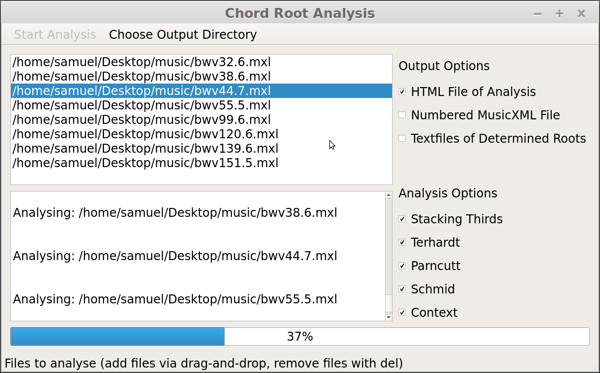
Figure 6.1: A screenshot of the program during analysis.

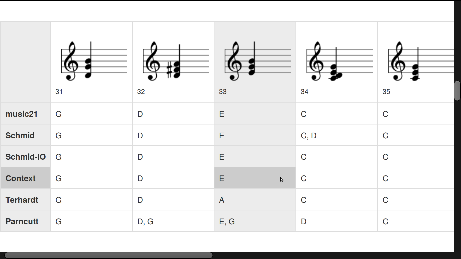
Figure 6.2: A screenshot of the HTML output of parts of BWV 99.6 (in G major).

Note that the displayed notes only represent the pitch classes of the chords.
The bass notes are $G$, $F\sharp$, $E$, $B$ and $C$.

Chapter 7 Conclusion and Future Work

7.1 Conclusion

In this thesis we first gave a basic introduction to music theory and in particular chord roots, for which we described several existing techniques on how to determine them. Then we introduced the newly developed Schmid model and showed how we extended it by exploiting sequential context to predict nonharmonic tones from a Computer Science perspective. Lastly, we implemented all the models and showed how researchers can use the program to do their own analyses of musical pieces.

A big hurdle for using machine learning algorithms for automatic feature extraction and classification is the lack of training data. If one day we have enough annotated data, it might be possible to use an automatic feature extraction and classification algorithm to directly determine chord roots from sequences of chords, but for this thesis we had to do a lot more manual work: First we searched for possible features of chord pairs and then we built a decision tree by hand, which works moderately well for pieces from Bach, but will probably fail for pieces from many different musical epochs.

7.2 Future Work

A small step has been done towards a better understanding of chord roots, but we are still very far away from a unifying model that works for all kinds of music. (Which would be more preferable than developing different theories for different kinds of music.)

While working on this thesis we came across several questions, which can not yet be answered conclusively and need addressing (Schmid, 2015, personal conversation):

• How do the new models hold up in empirical studies using both tonal and atonal music from different musical epochs?

• In what way do humans perceive chord roots and in what role do they play in the perception of music? Are they primarily a music theoretical concept?

• Until what maximum time interval does the human ear perceive tones that sound immediately after each other as chord? Is the perception of chord roots different when the notes do not sound at the same time?

• How important is sequential context for the determination of chord roots? How big can such a context be and how do we identify its boundaries?

• Is it possible to always correctly predict a single root when a chord is embedded in some sequential harmonic context or can it still be ambiguous?

• Are absolute pitches important? Are the heights of pitches relative to each other important? (c.f. Figure 4.4)

• In what way do different musical parameters (tone color, rhythm, dynamic, …) influence the perception of chord roots?

Appendix A List of Intervals

Table A.1 shows the names of different intervals. $N$ shows the number of semitones (i.e. the distance between two notes on the piano keyboard counting black as well as white keys) and $M$ shows the number of diatonic steps (i.e. the distance between two notes on the piano keyboard only counting the white keys, or the number of name changes between the notes ignoring accidentals). In the left table the intervals are sorted by diatonic steps and in the right table they are sorted by semitones.

$M$	$N$	Interval
0	0	Perfect unison
	1	Augmented unison
1	0	Diminished second
	1	Minor second
	2	Major second
	3	Augmented second
2	2	Diminished third
	3	Minor third
	4	Major third
	5	Augmented third
3	4	Diminished fourth
	5	Perfect fourth
	6	Augmented fourth
4	6	Diminished fifth
	7	Perfect fifth
	8	Augmented fifth
5	7	Diminished sixth
	8	Minor sixth
	9	Major sixth
	10	Augmented sixth
6	9	Diminished seventh
	10	Minor seventh
	11	Major seventh
	12	Augmented seventh
7	11	Diminished octave
	12	Perfect octave

$N$	$M$	Interval
0	0	Perfect unison
	1	Diminished second
1	1	Minor second
	0	Augmented unison
2	1	Major second
	2	Diminished third
3	2	Minor third
	1	Augmented second
4	3	Major third
	4	Diminished fourth
5	3	Perfect fourth
	2	Augmented third
6	4	Diminished fifth
	3	Augmented fourth
7	4	Perfect fifth
	5	Diminished sixth
8	5	Minor sixth
	4	Augmented fifth
9	5	Major sixth
	6	Diminished seventh
10	6	Minor seventh
	5	Augmented sixth
11	6	Major seventh
	7	Diminished octave
12	7	Perfect octave
	6	Augmented seventh

Table A.1: Interval names and their corresponding diatonic steps and semitones.

Appendix B Benchmarks

Piece	ST	Schmid	IO	Context	Auto	Terhardt	Parncutt
BWV 5.7	86.44	83.05	84.75	98.31	83.05	42.37	61.02
BWV 6.6	83.33	79.63	81.48	96.30	87.04	42.59	68.52
BWV 10.7	97.92	93.75	93.75	97.92	93.75	62.50	56.25
BWV 13.6	86.89	80.33	81.97	98.36	96.72	59.02	55.74
BWV 14.5	83.33	80.00	80.00	100.00	85.56	41.11	60.00
BWV 17.7	88.98	86.51	86.51	96.03	88.10	58.73	54.76
BWV 18.5	81.31	71.03	71.96	93.46	74.77	30.84	57.94
BWV 20.7	86.02	77.42	77.42	93.55	80.65	43.01	51.61
BWV 26.6	82.26	82.26	82.26	91.94	83.87	45.16	72.58
BWV 32.6	80.21	72.92	73.96	100.00	81.25	59.38	59.38
BWV 38.6	87.84	86.49	87.84	98.65	75.68	36.49	63.51
BWV 44.7	85.00	83.33	83.33	98.33	98.33	50.00	43.33
BWV 55.5	84.95	76.34	79.57	100.00	84.95	44.09	55.91
BWV 99.6	85.14	75.68	81.08	97.30	87.84	56.76	54.05
BWV 120.6	84.78	79.35	81.52	97.83	84.78	58.70	59.78
BWV 139.6	81.94	73.61	76.39	98.61	87.50	48.61	51.17
BWV 151.5	86.54	75.00	78.85	90.38	86.54	55.77	50.00
BWV 190.7	96.52	96.52	96.52	100.00	98.26	64.35	50.43
BWV 244.15	89.74	78.21	80.77	93.59	80.77	53.85	53.85
BWV 244.54	85.53	76.32	76.32	94.74	90.79	44.74	63.16
BWV 310	86.00	80.00	82.00	96.00	86.00	44.00	72.00
BWV 312	77.05	76.23	76.23	90.16	80.33	33.61	67.21
BWV 418	94.12	90.59	91.76	95.29	88.24	52.94	55.29
BWV 419	87.36	77.01	78.16	87.36	72.41	29.89	62.07
BWV 429	86.21	79.31	82.76	90.80	86.21	57.47	54.02
BWV 438	89.80	73.47	79.59	79.59	73.47	55.10	65.31
Overall	86.13	80.21	81.67	95.34	85.01	48.59	58.20

Table B.1: Achieved correctness of the different corpus on the annotated Bach corpus in percent.

“ST” is stacking thirds, “IO” is the Schmid model with an interval order and “Auto” is the Context model with the automatically generated decision tree. The annotated corpus contains question marks for some chords of which the correct roots were unknown. These chords are ignored for this benchmark.

Appendix C List of Program Options

To get a list of all possible options, we can use the “help” flag, which will give us a detailed description.

⬇

$ python3 analyse.py -h

The general usage of the program is

⬇

$ python3 analyse.py INPUT [OPTIONS]

Option (Short Option)	Description
--help (-h)	Show a help message and exit
--filetype (-t) FILETYPE	Set the filetype of the files that will be read in from the input-
	directory (default is .mxl)
--outdir (-o) OUTDIR	Choose the output-directory (By default all outputfiles will be
	placed in the same directory as the input-files)
--models (-m) MODELS	Choose the models with which the pieces will be analysed.
	MODELS should be a string containing the model-names
	seperated by whitespaces.
	E.g.: ’music21 Parncutt Terhardt Schmid Context’
--nohtmls	Do not output HTML file of the analysis
--musicxmls (-mx)	Output a numbered MusicXML file for each inputfile
--txts	For each inputfile write out .txt files for each models contain-
	ing the predicted roots (one root per line)
--statistics (-s)	Calculate and display statistics of correctly predicted roots for
	each model. This needs a .txt file for each inputfile where the
	correct roots are contained (one root per line). The name of
	the file should be
	name_of_inputfile_without_suffix + .correct.txt
--debug (-d)	Display debug messages
--verbose (-v)	Increase the output verbosity

Table C.1: List of possible program options.

References

- Bootstrap Development Team (2015) Bootstrap Development Team. Bootstrap HTML, CSS, and JS framework, 2015. Available at http://getbootstrap.com/, accessed on June 5th 2015.
- Cuthbert (2010) Christopher Cuthbert, Michael Scott; Ariza. music21: A Toolkit for Computer-Aided Musicology and Symbolic Music Data. In ISMIR 2010 : proceedings of the 11th International Society for Music Information Retrieval Conference, August 9-13, 2010, Utrecht, Netherlands, 2010. ISBN 9789039353813. Available at http://web.mit.edu/music21/, version 2.0.4, accessed on June 5th 2015.
- Forte (1973) Allen Forte. The structure of atonal music. Yale University Press, New Haven, 1973. ISBN 978-0300021202.
- Goldbach (2009) Karl Traugott Goldbach. Modelle der Akkordgrundtonbestimmung. Zeitschrift der Gesellschaft für Musiktheorie (ZGMTH), 6/2-3:385–422, 2009.
- Grabner (1974) Hermann Grabner. Allgemeine Musiklehre. Bärenreiter, Kassel, 1974. ISBN 978-3761800614.
- Hindemith (1942) Paul Hindemith. The craft of musical composition. Schott, Mainz New York, 1942. ISBN 0901938300.
- jQuery Foundation (2015) jQuery Foundation. jQuery JavaScript library, version 1.11.1, 2015. Available at https://jquery.com/, accessed on June 5th 2015.
- Parncutt (1997) Richard Parncutt. A model of the perceptual root(s) of a chord accounting for voicing and prevailing tonality. Music, Gestalt, and Computing, pages 181–199, 1997. 10.1007/BFb0034114.
- Pedregosa et al. (2011) F. Pedregosa, G. Varoquaux, A. Gramfort, V. Michel, B. Thirion, O. Grisel, M. Blondel, P. Prettenhofer, R. Weiss, V. Dubourg, J. Vanderplas, A. Passos, D. Cournapeau, M. Brucher, M. Perrot, and E. Duchesnay. Scikit-learn: Machine learning in Python. Journal of Machine Learning Research, 12:2825–2830, 2011.
- Python Software Foundation (2015) Python Software Foundation. Python Programming Language, version 3.4.0, 2015. Available at https://www.python.org/, accessed on June 5th 2015.
- Rameau (1971) Jean-Philippe Rameau. Treatise on harmony (1722). Dover Publications, New York, 1971. ISBN 978-0486224619.
- Riverbank Computing (2015) Riverbank Computing. Pyqt, version 5, 2015. Available at www.riverbankcomputing.com/, accessed on June 5th 2015.
- Roederer (2000) Juan G. Roederer. Physikalische und psychoakustische Grundlagen der Musik. Springer Berlin Heidelberg, Berlin, Heidelberg, 2000. ISBN 978-3-642-57138-1.
- Schmid (2014) Martin Anton Schmid. Akkordgrundton - musiktheoretisches Konzept und interdisziplinäres Forschungsfeld, 2014. URL http://www.martinantonschmid.at/uploads/2/0/8/7/20871030/20141017-vortrag-textversion.pdf. Talk at the public course “Musik und Psyche” at the Tiroler Landeskonservatorium, Innsbruck, Austria, Accessed on June 5th 2015.
- Schönberg (1969) Arnold Schönberg. Structural functions of harmony. W.W. Norton, New York, 1969. ISBN 978-0393004786.
- Schönberg (2010) Arnold Schönberg. Theory of harmony. University of California, Berkeley, Calif, 2010. ISBN 978-0520266087.
- Terhardt (1982) Ernst Terhardt. Die psychoakustischen Grundlagen der musikalischen Akkordgrundtöne und deren algorithmische Bestimmung. In Tiefenstruktur der Musik, Festschrift., pages 23–50. Terhardt, E., 1982.
- Utgoff (1996) Paul E Utgoff. ELF: An evaluation function learner that constructs its own features. 1996. University of Massachusetts.
- VexFlow Development Team (2015) VexFlow Development Team. VexFlow JavaScript library, version 1.2.26, 2015. Available at http://www.vexflow.com/, accessed on June 5th 2015.
- Ziegenrücker (2009) Wieland Ziegenrücker. ABC Musik allgemeine Musiklehre ; 446 Lehr- und Lernsätze. Breitkopf und Härtel, Leipzig, 2009. ISBN 978-3765103094.