Wigner Functions for the Pair Angle and Orbital Angular Momentum

Abstract

The problem of constructing physically and mathematically well-defined Wigner functions for the canonical pair angle $\theta$ and angular momentum $p$ is solved. While a key element for the construction of Wigner functions for the planar phase space $\{(q,p)\in\mathbb{R}^{2}\}$ is the Heisenberg-Weyl group, the corresponding group for the cylindrical phase space $\{(\theta,p)\in S^{1}\times\mathbb{R}\}$ is the Euclidean group $E(2)$ of the plane and its unitary representations. Here the angle $\theta$ is replaced by the pair $(\cos\theta,\sin\theta)$ which corresponds uniquely to the points on the unit circle. The main structural properties of the Wigner functions for the planar and the cylindrical phase spaces are strikingly similar.

A crucial role plays the $\operatorname{sinc}$ function which provides the interpolation for the discontinuous quantized angular momenta in terms of the continuous classical ones, in accordance with the famous Whittaker cardinal function well-known from interpolation and sampling theories.

The quantum mechanical marginal distributions for angle (continuous) and angular momentum (discontinuous) are as usual uniquely obtained by appropriate integrations of the $(\theta,p)$ Wigner function. Among the examples discussed is an elementary system of simple ”cat” states.

I Introduction

In 1932 Wigner introduced a function on the classical $(q,p)$ phase space of a given system with the aim to describe quantum mechanical statistical properties of that system partially in terms of classical ones Wigner (1932); Hillery et al. (1984). After a slow start the concept has become quite popular and efficient, e.g. in quantum optics Leonhardt (1997); Schleich (2001); Römer (2009); Leonhardt (2010); Agarwal (2013) and time-frequency analysis Gröchenig (2001); Cohen (2013).

In view of the successes of Wigner functions on the topologically trivial planar phase space $\mathbb{R}^{2}$ attempts have been made to generalize the concept to other phase spaces, in particular to that of a simple rotator around a fixed axis, its position given by an angle $\theta$ and its angular momentum by a real number $p$, thus having a phase space corresponding topologically to a cylinder of infinite length, i.e. $S^{1}\times\mathbb{R}$ .

A considerable obstacle for the quantum theory of that space is the treatment of the angle which has no satisfactory self-adjoint operator counterpart quantum mechanically Kastrup (2006). Nevertheless a “Hermitian” angle operator was introduced formally, exponentiated to a seemingly unitary one, and the classically continuous angular momentum $p$ was replaced by the discrete quantum mechanical $l\in\mathbb{Z}$ one, thus quantizing a hybrid “phase space” $S^{1}\times\mathbb{Z}$. This approach was started by Berry Berry (1977) and Mukunda Mukunda (1979) and has since been pursued by quite a number of authors. Typical more recent examples are Refs. Rigas et al. (2011); Przanowski et al. (2014); Mukunda et al. (2005).

The present paper provides consistant Wigner functions on the classical physical phase space $S^{1}\times\mathbb{R}$ including a mathematically satisfactory treatment of the angle $\theta\in\mathbb{S}^{1}$.

We shall see below (Subsec. II.B.) where the “hybrid” case $S^{1}\times\mathbb{Z}$ is to be placed within the framework proposed here.

Parallel to those attempts to find Wigner functions for systems on the cylinder its quantum mechanics was described – in two different approaches – surprisingly in terms of unitary representations of the Euclidean group $E(2)$ of the plane! Fronsdal initiated the first of these two in the framework of the so-called Moyal or $\star$ quantization Fronsdal (1979), followed by a number of papers by other authors, e.g. Gadella et al. (1991); Arratia and del Olmo (1997).

In a different approach Isham discussed very convincingly Isham (1984) the group theoretical quantization of the phase space $S^{1}\times\mathbb{R}$ in terms of irreducible unitary representations of $E(2)$ and its covering groups. His results could be used in order to discuss in detail the appropriate quantum mechanics of the $(\theta,p)$-rotator Kastrup (2006).

The present paper is a continuation of Ref. Kastrup (2006). It provides a mathematically and physically consistent Wigner function on a cylindrical phase space by utilizing the tools discussed in Ref. Kastrup (2006): Representing the angle $\theta$ of the rotator by the equivalent pair $(\cos\theta,\sin\theta)$ introduces - together with the angular momentum $p$ - simultaneously the 3-dimensional Lie algebra of the Euclidean group $E(2)$ in 2 dimensions. Unitary representations of that group provide the appropriate quantum mechanics of the rotator. Using slightly modified ideas for constructing “Wigner operators” from the Lie algebra of associated groups by Wolf and collaborators Wolf (1996); Nieto et al. (1998); Ali et al. (2000) leads to the corresponding operator $V(\theta,p)$ in terms of the Lie algebra of $E(2)$ (Sec. II). Wigner functions are obtained by calculating matrix elements of that operator within an irreducible representation of $E(2)$. Matrix elements between two different states yield Wigner-Moyal functions Moyal (1949) whereas two identical states provide Wigner functions proper Wigner (1932), the latter being a special case of the former.

The resulting structures and properties (Sec. III) have a very remarkable resemblence to those of the well-known $(q,p)$ case (for reviews see, e.g. Refs. Hillery et al. (1984); Folland (1989); de Gosson (2006)). An essential feature of the $(\theta,p)$ Wigner-Moyal functions is the central role played by the sinc function (sinus cardinalis)

$$\operatorname{sinc}\pi(p-m)=\frac{\sin\pi(p-m)}{\pi(p-m)},\,\,p\in\mathbb{R},\,m\in\mathbb{Z},$$ (1)

which interpolates between the discontinuous quantized angular momenta $m$ ($\hbar=1)$ by means of the continuous classical ones $p$ (for a graph of the function (1) see FIG.1 in Subsection IV.C. below).

In 1915 E.T. Whittaker introduced his - by now famous - cardinal function Whittaker (1915) for the continuous interpolation of functions for which discrete values are known by using the functions (1). Since then those functions have been playing an increasingly important role in the fields of interpolation, sampling and signal processing theories (see the reviews McNamee et al. (1971); Stenger (1981); Butzer (1983); Higgins (1985); Stenger (1993, 2011); Vetterli et al. (2014); Eldar (2015)).

The time evolution of Wigner-Moyal functions is determined by the Hermitian operator $K(\theta,p)=i[H,V(\theta,p)]$ (Sec. III.C.).

The quantum mechanical marginal distributions $|\psi(\theta)|^{2}$ and $b_{m}=|c_{m}|^{2}$, where the $c_{m}$ are the expansion coefficients of the wave function $\psi(\varphi)$ with respect to the basis $e_{m}(\varphi)=\exp(im\varphi),\,m\in\mathbb{Z}$, are obtained - as usual - by integrating the Wigner function $V_{\psi}(\theta,p)$ over $p$ and $\theta$ respectively. The latter integration yields a cardinal function $\omega_{\psi}(p)$ from which the probabilities $b_{m}$ can be extracted by means of the orthonormality of the $\operatorname{sinc}$ functions (1) (Sec. IV.B.).

Four examples of Wigner functions for certain typical states are discussed in Sec. IV.C.: That of the basis function $e_{m}(\varphi)$, that of the ”cat” state $(e_{1}(\varphi)+e_{-1}(\varphi))/\sqrt{2}$, that of ”minimal uncertainty” states $\psi_{e}(\varphi)$ which lead to the von Mises statistical distribution $|\psi_{e}(\varphi)|^{2}=\exp(2s\cos\varphi)/I_{0}(2s)$ and which are the analogue of the Gaussian wave packets in the $(q,p)$ case and finally that of thermal states associated with the Hamiltonian $H=\varepsilon L^{2}$, where $L$ is the quantum mechanical counterpart of the classical angular momentum $p$.

II The auxiliary role of the Euclidean group $\mathbf{E(2)}$

The close relationship between the rotator and the group $E(2)$ comes about as follows Kastrup (2006): In order to avoid the problems with a quantization of the angle $\theta$ itself Louisell and Mackey in 1963 suggested independently Louisell (1963); Mackey (1963) to use the pair $(\cos\theta,\sin\theta)$ instead, because it is in one-to-one correspondence to the points on the unit circle and it consists of smooth bounded $2\pi$-periodic functions the quantization of which appears most likely to be easier to handle than that for the angle itself.

II.1 Classical $\mathbf{E(2)}$ group theory

The basic functions

$$\tilde{h}_{1}=\cos\theta,\qquad\tilde{h}_{2}=\sin\theta,\qquad\tilde{h}_{3}=p_{\theta}\equiv p$$ (2)

on the classical phase space

$$\mathcal{S}_{\theta,p}=\{s=(\theta,p);\,\theta\in\mathbb{R}\,\bmod{2\pi},\,p\in\mathbb{R}\,\}$$ (3)

obey the Poisson brackets

$$\{\tilde{h}_{3},\tilde{h}_{1}\}_{\theta,p}=\tilde{h}_{2},\,\{\tilde{h}_{3},\tilde{h}_{2}\}_{\theta,p}=-\tilde{h}_{1},\,\{\tilde{h}_{1},\tilde{h}_{2}\}_{\theta,p}=0.$$ (4)

They constitute the Lie algebra of the 3-parametric Euclidean group $E(2)=\{g(\vartheta,\vec{a})\}$ of the plane:
$\vec{x}\rightarrow R(\vartheta)\cdot\vec{x}+\vec{a}$, i.e.

$$g(\vartheta,\vec{a})\circ\vec{x}=\begin{pmatrix}\cos\vartheta&-\sin\vartheta\\ \sin\vartheta&\cos\vartheta\end{pmatrix}\begin{pmatrix}x_{1}\\ x_{2}\end{pmatrix}+\begin{pmatrix}a_{1}\\ a_{2}\end{pmatrix}\,.$$ (5)

We write

$$\begin{pmatrix}\cos\vartheta&-\sin\vartheta\\ \sin\vartheta&\cos\vartheta\end{pmatrix}\begin{pmatrix}x_{1}\\ x_{2}\end{pmatrix}\equiv R(\vartheta)\vec{x}\equiv\vec{x}_{\vartheta}\,.$$ (6)

In the following it is advantageous to cast the relations (5) into those of $3\times 3$ matrices Vilenkin (1968), for which group multiplication etc. is implemented by matrix multiplication etc.:

$$g(\vartheta,\vec{a})\circ\begin{pmatrix}x_{1}\\ x_{2}\\ 1\end{pmatrix}=\left(\begin{array}[]{ccr}\cos\vartheta&-\sin\vartheta&a_{1}\\ \sin\vartheta&\cos\vartheta&a_{2}\\ 0&0&1\end{array}\right)\begin{pmatrix}x_{1}\\ x_{2}\\ 1\end{pmatrix}\,,$$ (7)

from which one can read off immediately the Lie algebra generators

$$\tilde{L}=\left(\begin{array}[]{ccr}0&-1&0\\ 1&0&0\\ 0&0&0\end{array}\right)\!,\,\tilde{K}_{1}=\left(\begin{array}[]{ccr}0&0&1\\ 0&0&0\\ 0&0&0\end{array}\right)\!,\,\tilde{K}_{2}=\left(\begin{array}[]{ccr}0&0&0\\ 0&0&1\\ 0&0&0\end{array}\right)\!.$$ (8)

They obey the commutation relations

$$[\tilde{L},\tilde{K}_{1}]=\tilde{K}_{2},~{}~{}[\tilde{L},\tilde{K}_{2}]=-\tilde{K}_{1},~{}~{}[\tilde{K}_{1},\tilde{K}_{2}]=0~{}.$$ (9)

These are obviously isomorphic to those of Eq.(4). In the corresponding quantum theory the generators $\tilde{L}$ and $\vec{\tilde{K}}=(\tilde{K}_{1},\tilde{K}_{2})$ will turn into self-adjoint operators $L$ and $\vec{K}$ which describe the quantum mecchanics of the angular momentum $p$ and the pair $(\cos\theta,\sin\theta)$.

As to the latter there is the following subtlety: In Eqs.(9) the generators $\tilde{K}_{j}$ are not normalized: If one multiplies them with a nonzero constant the new $\tilde{K}_{j}$ obey the same communitation relations as the old ones. This means that the relevant classical observable here is a direction, a vector (e.g. $\in\mathbb{C}$) or a half-ray

$$\vec{\chi}\,(\theta)=\chi\,(\cos\theta,\sin\theta)\,,\,\chi>0\,,$$ (10)

which carries all the required information on the angle $\theta$!

In the corresponding quantum theory the eigenvalues of $\vec{K}$ are

$$\vec{k}(\varphi)=k\,(\cos\varphi,\sin\varphi)\,,\,k>0\,,$$ (11)

with $k^{2}$ the value of the Casimir operator $\vec{K}^{2}$; therefore $k$ is not “quantized”. It also characterizes the irreducible unitary representations of $E(2)$ Isham (1984); Vilenkin (1968); Sugiura (1990). We shall see below that the modulus $k$ can easily be integrated out with only the essential pair $(\cos\theta,\sin\theta)$ left.

Using series expansion for the exponentials we get

$$g(\vartheta,\vec{a}=0)=g(\vartheta)=e^{\displaystyle\vartheta\tilde{L}}=\left(\begin{array}[]{ccr}\cos\vartheta&-\sin\vartheta&0\\ \sin\vartheta&\cos\vartheta&0\\ 0&0&1\end{array}\right)\,,$$ (12)

$$g(\vartheta=0,a_{1},a_{2}=0)=g(a_{1})=e^{\displaystyle a_{1}\tilde{K}_{1}}=\begin{pmatrix}1&0&a_{1}\\ 0&1&0\\ 0&0&1\end{pmatrix}\,,$$ (13)

$$g(\vartheta=0,a_{1}=0,a_{2})=g(a_{2})=e^{\displaystyle a_{2}\tilde{K}_{2}}=\begin{pmatrix}1&0&0\\ 0&1&a_{2}\\ 0&0&1\end{pmatrix}\,.$$ (14)

The group element in relation (7) can then be written as

$$g(\vartheta,\vec{a})=g(a_{2})\circ g(a_{1})\circ g(\vartheta)\,.$$ (15)

We now arrive at a critical part of the paper: Like in the case of the Heisenberg-Weyl group Folland (1989); de Gosson (2006) the special group element Nieto et al. (1998); Chirikjian and Kyatkin (2000)

$$g_{0}(\vartheta,\vec{b}) =\exp(b_{1}\tilde{K}_{1}+b_{2}\tilde{K}_{2}+\vartheta\tilde{L})$$

$$=\begin{pmatrix}\lx@intercol\hfil R(\vartheta)\hfil\lx@intercol&\operatorname{sinc}(\vartheta/2)\,R(\vartheta/2)\vec{b}\\ 0&0&1\end{pmatrix}$$ (16)

plays an essential role in the following construction of the Wigner function. Its importance was emphasized previously by Wolf and collaborators Wolf (1996); Nieto et al. (1998); Ali et al. (2000).

Comparing Eq.(II.1) and Eq.(7) shows that the translations are now parametrized in an angle dependent way. We have

$$\vec{a}=\operatorname{sinc}(\vartheta/2)\,R(\vartheta/2)\vec{b}\,.$$ (17)

Crucial for the rest of the paper is that the element $g_{0}$ from Eq. (II.1) can also be written as

$$g_{0}(\vartheta,\vec{b})=e^{\displaystyle(\vartheta/2)\tilde{L}}\circ e^{\displaystyle\operatorname{sinc}(\vartheta/2)\,\vec{b}\cdot\vec{\tilde{K}}}\circ e^{\displaystyle(\vartheta/2)\tilde{L}}\,,$$ (18)

which amounts to a kind of Weyl symmetrization! From Eq. (17) we then obtain

$$g_{0}(\vartheta,\vec{a})=e^{\displaystyle(\vartheta/2)\tilde{L}}\circ e^{\displaystyle R(-\vartheta/2)\vec{a}\cdot\vec{\tilde{K}}}\circ e^{\displaystyle(\vartheta/2)\tilde{L}}\,.$$ (19)

Now the undesirable factor $\operatorname{sinc}(\vartheta/2)$ has dropped out.

II.2 Constructing the quantum mechanical
Wigner operator

In the quantum theory the group element (19) is “promoted” to the unitary operator

$$U_{0}(\vartheta,\vec{a})=e^{\displaystyle i(\vartheta/2)L}\circ e^{\displaystyle i\vec{a}_{(-\vartheta/2)}\cdot\vec{K}}\circ e^{\displaystyle i(\vartheta/2)L}\,.$$ (20)

(See Eq. (6) as to notations.)

The unitary operator $U_{0}$ is supposed to act in an appropriate Hilbert space in which the Euclidean group is represented unitarily and in which the operators $L$, $K_{1}$ and $K_{2}$ are self-adjoint. Possible unitary representations are the irreducible, the quasi-regular and the regular ones Vilenkin (1968). We here consider only irreducible unitary representations of $E(2)$ Vilenkin (1968); Isham (1984); Sugiura (1990); Chirikjian and Kyatkin (2000).

For the construction of appropriate Wigner functions on the phase space (3) we have to combine the operator (20) in a suitable way with the classical variables $\vec{\chi}(\theta)$ (see Eq.(10)) and the angular momentum $p$ . Following lessons from the Heisenberg-Weyl group Folland (1989); de Gosson (2006) and from – appropriately modified – suggestions by Wolf et al. Wolf (1996); Nieto et al. (1998) the present proposal as to a proper $(\theta,p)$ Wigner operator for the phase space with the topology $S^{1}\times\mathbb{R}$ is

$$V[\vec{\chi}(\theta),p]=\frac{1}{(2\pi)^{3}}\int_{-\pi}^{\pi}\!d\vartheta\int_{-\infty}^{\infty}\!da_{1}da_{2}\,\hat{U}_{0}\,,$$ (21)

$$\hat{U}_{0}=e^{\displaystyle i(L-p)(\vartheta/2)}\circ e^{\displaystyle i(\vec{K}-\vec{\chi}(\theta))\cdot\vec{a}_{(-\vartheta/2)}}$$

$$\circ\,e^{\displaystyle i(L-p)(\vartheta/2)}\,.$$

This is a kind of ordered group averaging (with invariant Haar measure $dg(\vartheta,\vec{a})=d\vartheta da_{1}da_{2}\,$) of the differences between the classical quantities $\vec{\chi}(\theta)$ and $p$ and their corresponding operator counterparts.

The ansatz (21) differs from that of Ref. Nieto et al. (1998) essentially by a different operator ordering which avoids the obstructive explicit factor $\operatorname{sinc}(\vartheta/2)$ .

All irreducible unitary representations of $E(2)$ and its – infinitely many – covering groups can be implemented in a Hilbert space $L^{2}(S^{1},d\varphi/2\pi;\delta)$ with the scalar product

$$(\psi_{2},\psi_{1})=\int_{-\pi}^{\pi}\frac{d\varphi}{2\pi}\psi_{2}^{\ast}(\varphi)\psi_{1}(\varphi)\,,$$ (22)

and a basis

$$e_{n,\delta}(\varphi)=e^{\displaystyle i(n+\delta)\varphi}\,,(e_{m,\delta},e_{n,\delta})=\delta_{mn},\,m,n\in\mathbb{Z}\,,$$ (23)

where $\delta\in[0,1)$ characterizes the choice of a covering group Kastrup (2006); Isham (1984). A $\delta\neq 0$ becomes important for fractional orbital angular momenta Kastrup (2006). $\delta_{mn}$ is, of course, the usual Kronecker symbol.

For any $\psi^{[\delta]}(\varphi)\in L^{2}(S^{1},d\varphi/2\pi;\delta)$, i.e. $\psi^{[\delta]}(\varphi+2\pi)=e^{i2\pi\delta}\psi^{[\delta]}(\varphi)$ we have the expansion

$$\psi^{[\delta]}(\varphi)=\sum_{n\in\mathbb{Z}}c_{n}\,e_{n,\delta}(\varphi)\,,~{}c_{n}=(e_{n,\delta},\psi^{[\delta]})\,.$$ (24)

The coefficients $c_{n}$ are independent of $\delta$! That dependence of $\psi^{[\delta]}(\varphi)$ is taken over by the $e_{n,\delta}(\varphi)$.

In the following we put $\delta=0$. The general case $\delta\neq 0$ will be briefly discussed in Subsection V.A. below.

The action of the self-adjoint operators $\vec{K}$ and $L$ is given by ($\hbar$ =1)

$$\vec{K}\psi(\varphi)=k\,(\cos\varphi,\sin\varphi)\,\psi(\varphi)\,,~{}~{}L\psi(\varphi)=\frac{1}{i}\partial_{\varphi}\psi(\varphi)\,,$$ (25)

$$e^{\displaystyle i\vec{a}_{(-\vartheta/2)}\cdot\vec{K}}\psi(\varphi) = e^{\displaystyle i\vec{a}_{(-\vartheta/2)}\cdot\vec{k}(\varphi)}\psi(\varphi)\,,$$ (26)

$$e^{\displaystyle i\vartheta L}\psi(\varphi) = \psi(\varphi+\vartheta)\,.$$ (27)

The functions $e_{n,\delta}(\varphi)$ obviously are eigenfunctions of $L$ with eigenvalues $n+\delta$ whereas $\vec{K}$ acts as a multiplication operator.

Different values of $k$ belong to different irreducible representations and the Plancherel measure for the Fourier transforms on $E(2)$ is $k\,dk\,$Vilenkin (1968); Sugiura (1990); Chirikjian and Kyatkin (2000).

We here can see what the replacement of the proper classical phase space $S^{1}\times\mathbb{R}$ by $S^{1}\times\mathbb{Z}$ means (see also Ref. Kastrup (2006)): it amounts to putting $k=0$ in Eqs. (25) and (26), i.e. representing the translations of $E(2)$ – which correspond to the pair $(\cos\theta,\sin\theta)$ – by the identity (the translations form a normal subgroup). Thus eliminating the observable “angle” altogether! What is left are infinitely many irreducible representations $\{e^{in\varphi},n\in\mathbb{Z}\}$ of $SO(2)$ alone and the factor $\mathbb{Z}$ in $S^{1}\times\mathbb{Z}$ corresponds to that dual of $SO(2)$. The angle $\theta$ then has to be introduced forcibly “by hand”!

For the matrix elements

$$V^{(k)}_{\psi_{2}\psi_{1}}[\vec{\chi}(\theta),p]\equiv(\psi_{2},V[\vec{\chi}(\theta),p]\psi_{1})$$ (28)

we obtain from the relations (26) and (27):

$$V^{(k)}_{\psi_{2}\psi_{1}}[\vec{\chi}(\theta),p]=\frac{1}{(2\pi)^{4}}\int\!dg(\vartheta,\vec{a})\,d\varphi\,e^{\displaystyle-i\omega+\vec{k}(\varphi)\vec{a}_{(-\vartheta/2)}}$$

$$\times\psi_{2}^{\ast}(\varphi-\vartheta/2)\psi_{1}(\varphi+\vartheta/2)\,,\,\omega=\vec{\chi}(\theta)\cdot\vec{a}_{(-\vartheta/2)}+p\,\vartheta\,.$$ (29)

Introducing polar coordinates $\vec{a}=a\,(\cos\alpha,\sin\alpha)$ yields

$$V^{(k)}_{\psi_{2}\psi_{1}} = \frac{1}{(2\pi)^{4}}\int d\vartheta\,d\alpha\,ada\,d\varphi\,e^{\displaystyle-ip\,\vartheta}\times$$

$$e^{\displaystyle-ia\chi\cos(\theta-\alpha+\vartheta/2)}e^{\displaystyle iak\cos(\varphi-\alpha+\vartheta/2)}\times$$

$$\psi_{2}^{\ast}(\varphi-\vartheta/2)\psi_{1}(\varphi+\vartheta/2)\,.$$

Because of the possible expansion (24) it suffices to take $\psi_{2}(\varphi)=e_{m}(\varphi)$ and $\psi_{1}(\varphi)=e_{n}(\varphi)$.

Recalling the integral representation

$$J_{n}(x)=\frac{1}{2\pi}\int_{-\pi}^{\pi}d\beta e^{\displaystyle i(x\,\sin\beta-n\,\beta)},\,n\in\mathbb{Z},$$ (31)

of the Bessel functions Whittaker and Watson (1969), their (Hankel transform) ”completeness” relation Morse and Feshbach (1953)

$$\int_{0}^{\infty}da\,a\,J_{m}(x\,a)\,J_{m}(y\,a)=\frac{1}{x}\delta(x-y)$$ (32)

and using the orthonormality (23) of the $e_{m}(\varphi)$ we finally get

$$V^{(k)}_{mn}(\theta,p) = e^{\displaystyle i(n-m)\theta}\left(\frac{1}{k}\delta(k-\chi)\right)\times$$

$$\frac{1}{(2\pi)^{2}}\int_{-\pi}^{\pi}d\vartheta\,e^{\displaystyle i[(m+n)/2-p]\vartheta}\,.$$

III Main results

III.1 The phase space Wigner-Moyal matrix

Eq. (II.2) shows explicitly that the scale factor $\chi$ is a redundent variable and can easily be eliminated: integration (averaging) with the Plancherel measure $k\,dk$ gives our surprisingly simple but powerful main result

$$V_{mn}(\theta,p)=\int_{0}^{\infty}dk\,kV^{(k)}_{mn}(\theta,p)=$$ (35)

$$=\frac{1}{(2\pi)^{2}}\,e^{\displaystyle i(n-m)\theta}\int_{-\pi}^{\pi}d\vartheta\,e^{\displaystyle i[(n+m)/2-p]\vartheta}$$

$$=\frac{1}{2\pi}\,e^{\displaystyle i(n-m)\theta}\,\operatorname{sinc}\pi[p-(m+n)/2]\,.$$

The infinite-dimensional Hermitian (Wigner-Moyal) matrix $V(\theta,p)=(V_{mn}(\theta,p))$ has the properties

$$\int_{-\infty}^{\infty}dp\,V_{mn}(\theta,p)=\frac{1}{2\pi}\,e^{\displaystyle i(n-m)\theta}\,,$$ (36)

$$\int_{-\pi}^{\pi}d\theta\,V_{mn}(\theta,p)=\operatorname{sinc}\pi(p-m)\,\delta_{mn}\,,$$ (37)

$$\int_{-\pi}^{\pi}d\theta\int_{-\infty}^{\infty}dp\,V_{mn}(\theta,p)=\delta_{mn}\,,$$ (38)

$$\operatorname{tr}(V_{mn}(\theta,p))=\frac{1}{2\pi}\sum_{n\in\mathbb{Z}}\operatorname{sinc}\pi(p-n)=\frac{1}{2\pi},$$ (39)

$$\int_{-\pi}^{\pi}d\theta\int_{-\infty}^{\infty}dp\,V_{kl}(\theta,p)\,V_{mn}(\theta,p)=\frac{1}{2\pi}\delta_{kn}\delta_{lm}\,,$$ (40)

$$|V_{mn}|\leq\frac{1}{2\pi}\,,$$ (41)

where the relations

$$\operatorname{sinc}\pi x = 1\mbox{ for }x=0\,,$$ (42)

$$|\operatorname{sinc}\pi x| < 1\mbox{ for }x\neq 0\,,$$

$$\int_{-\infty}^{\infty}dx\,\operatorname{sinc}\pi(x+a) = 1,\,a\in\mathbb{R}\,,$$ (43)

$$\frac{1}{2\pi}\sum_{n\in\mathbb{Z}}e^{\displaystyle in\beta}=\delta(\beta) \beta\in[-\pi,\,+\pi],$$ for (44)

have been used. For Eq. (39) see also Ref. Prudnikov et al. (1986).

It follows from Eq. (40) that

$$\int_{-\pi}^{\pi}d\theta\int_{-\infty}^{\infty}dp\,V^{T}(\theta,p)\cdot V(\theta,p) = \frac{1}{2\pi}\mathbf{1}\,,$$ (45)

$$\int_{-\pi}^{\pi}d\theta\int_{-\infty}^{\infty}dp\,V(\theta,p)\cdot V^{T}(\theta,p) = \frac{1}{2\pi}\mathbf{1}\,,$$ (46)

where $V^{T}(=V^{\ast})$ is the transpose of the matrix $V$ and $\mathbf{1}$ the unit operator in Hilbert space. Thus, $V$ is Hermitian and even orthogonal, but not unitary!

Another interesting property of $V(\theta,p)$ is

$$\operatorname{tr}[V(\theta_{1},p_{1})\cdot V(\theta_{2},p_{2})]=\frac{1}{2\pi}\,\delta(\theta_{1}-\theta_{2})\,\operatorname{sinc}\pi(p_{1}-p_{2})\,.$$ (47)

Integrating this equation over the pair $(\theta_{1},p_{1})$ (or $(\theta_{2},p_{2})$) consistently yields the relation (39).

As already mentioned in the Introduction the function $\operatorname{sinc}\pi(p-m)$ interpolates the discrete quantum numbers $m$ etc. in terms of the continuous classical variable $p$ (for more details see the discussion in Section IV below).

Notice the following difference as to integrations over angles above: whereas the integration measure in the scalar product (22) is normalized as $d\phi/(2\pi)$, the corresponding measure for the phase space angle variable $\theta$ is $d\theta$.

For expansions

$$\psi_{j}(\varphi)=\sum_{n\in\mathbb{Z}}c_{n}^{(j)}e_{n}(\varphi)\,,\,j=1,2;\,\,\,c_{n}^{(j)}=(e_{n},\psi_{j}),$$ (48)

we get the “Moyal” function (see Refs. Folland (1989); Schleich (2001); de Gosson (2006) as to the corresponding $(q,p)$ case)

$$V_{\psi_{2}\psi_{1}}(\theta,p)=\sum_{m,n\in\mathbb{Z}}c_{m}^{(2)\ast}V_{mn}(\theta,p)c_{n}^{(1)}$$ (49)

$$=\frac{1}{(2\pi)^{2}}\int_{-\pi}^{\pi}d\vartheta\,e^{\displaystyle-ip\vartheta}\psi_{2}^{\ast}(\theta-\vartheta/2)\,\psi_{1}(\theta+\vartheta/2)\,,$$

$$=(\psi_{2},V(\theta,p)\psi_{1})\,,$$

which, according to Eqs. (36) - (40), has the properties

$$\int_{-\infty}^{\infty}dp\,V_{\psi_{2}\psi_{1}}(\theta,p)=\frac{1}{2\pi}\psi_{2}^{\ast}(\theta)\,\psi_{1}(\theta)\,,$$ (50)

$$\int_{-\pi}^{\pi}d\theta\,V_{\psi_{2}\psi_{1}}(\theta,p)=\sum_{m\in\mathbb{Z}}c_{m}^{(2)\ast}\operatorname{sinc}\pi(p-m)c_{m}^{(1)}\,,$$ (51)

$$\int_{-\infty}^{\infty}dp\int_{-\pi}^{\pi}d\theta\,V_{\psi_{2}\psi_{1}}(\theta,p)=(\psi_{2},\psi_{1})\,,$$ (52)

$$\int_{-\infty}^{\infty}dp\int_{-\pi}^{\pi}d\theta\,V^{\ast}_{\psi_{2}\psi_{1}}(\theta,p)\,V_{\phi_{2}\phi_{1}}(\theta,p)=$$ (53)

$$=\frac{1}{2\pi}(\psi_{1},\phi_{1})\,(\psi_{2},\phi_{2})^{\ast}\,.$$

On the left hand sides of the Eqs. (50) - (53) we have integrals over phase space functions, whereas on the right hand ones we have quantities from the corresponding Hilbert space, except for Eq. (51) where the function $\operatorname{sinc}\pi(p-m)$ occurs. However, because of the orthonormality relation (References in Section IV below)

$$\int_{-\infty}^{\infty}dp\,\operatorname{sinc}\pi(m-p)\,\operatorname{sinc}\pi(n-p)=\delta_{mn}\,$$ (54)

that sinc-function can be eliminated immediately:

$$\int_{-\infty}^{\infty}dp\,\operatorname{sinc}\pi(n-p)\int_{-\pi}^{\pi}d\theta\,V_{\psi_{2}\psi_{1}}(\theta,p)=$$ (55)

$$\int_{-\infty}^{\infty}dp\,\operatorname{sinc}\pi(n-p)\sum_{m\in\mathbb{Z}}c_{m}^{(2)\ast}\operatorname{sinc}\pi(p-m)c_{m}^{(1)}=$$

$$=c_{n}^{(2)\ast}\,c_{n}^{(1)}\,,$$

a relation which will become important in Sec. IV for $\psi_{2}=\psi_{1}$.

III.2 Phase space functions associated with
Hilbert space operators

If $\psi_{1}(\varphi)=A\psi(\varphi)$, where $A$ is some operator, (e.g. $\cos\varphi,\,\sin\varphi,\,L$ or functions of these), then Eq. (52) provides matrix elements of $A$ and if $\psi_{2}=\psi$ its expectation value $(\psi,A\psi)$ in terms of integrals over phase space densities:

For $\psi_{1}=A\psi$ we have

$$c_{n}^{(1)}=\sum_{k\in\mathbb{Z}}c_{k}\,(e_{n},Ae_{k})$$ (56)

and it follows from Eq. (52) that

$$(\psi_{2},A\psi) = \int_{-\infty}^{\infty}dp\int_{-\pi}^{\pi}d\theta\,a_{\psi_{2}\psi}(\theta,p)\,,$$ (57)

$$a_{\psi_{2}\psi}(\theta,p) = \sum_{m,n\in\mathbb{Z}}\frac{1}{2}c^{(2)\ast}_{m}[V(\theta,p)\cdot A+A\cdot V(\theta,p)]_{mn}c_{n}\,,$$

which expresses a quantum mechanical matrix element in terms of a phase space integral over an associated density $a_{\psi_{2}\psi}(\theta,p)$! The (Weyl) symmetrization of $V=(V_{mk})$ and $A=(A_{kn})$ in Eq. (57) is required for $a_{\psi\psi}(\theta,p)$ to be real if $A$ is Hermitian!

For $\psi_{2}=e_{m},\psi=e_{n}$ we get

$$A_{mn} \equiv (e_{m},Ae_{n})=\int_{-\infty}^{\infty}dp\int_{-\pi}^{\pi}d\theta\,a_{mn}(\theta,p)\,,$$

$$a_{mn}(\theta,p) = \frac{1}{2}[V(\theta,p)\cdot A+A\cdot V(\theta,p)]_{mn}\,,$$ (58)

which can formally be written as

$$A=(A_{mn})=\int_{-\infty}^{\infty}dp\int_{-\pi}^{\pi}d\theta\,\frac{1}{2}[V(\theta,p)\cdot A+A\cdot V(\theta,p)]\,.$$ (59)

¿From the diagonal elements

$$a_{m}(\theta,p)=\frac{1}{2}[V(\theta,p)\cdot A+A\cdot V(\theta,p)]_{mm}$$ (60)

we obtain

$$\operatorname{tr}A= \sum_{m\in\mathbb{Z}}\int_{-\infty}^{\infty}dp\int_{-\pi}^{\pi}d\theta\,a_{m}(\theta,p)$$ (61)

$$= \int_{-\infty}^{\infty}dp\int_{-\pi}^{\pi}d\theta\,\operatorname{tr}[A\cdot V(\theta,p)]\,.$$

If $A$ is a diagonal density matrix

$$\rho=(\lambda_{n}\,\delta_{mn}),\,\lambda_{n}\geq 0,\,\sum_{n\in\mathbb{Z}}\lambda_{n}=1,$$ (62)

then we have

$$\operatorname{tr}[\rho\cdot V(\theta,p)]=\frac{1}{2\pi}\sum_{m\in\mathbb{Z}}\lambda_{m}\operatorname{sinc}\pi(p-m)\,,$$ (63)

$$\int_{-\infty}^{\infty}dp\int_{-\pi}^{\pi}d\theta\,\operatorname{tr}[\rho\cdot V(\theta,p)]=\sum_{m\in\mathbb{Z}}\lambda_{m}=1\,.$$ (64)

Using the relations (54) the probabiities $\lambda_{m}$ can be extracted from Eq. (63):

$$\lambda_{m}=2\pi\int_{-\infty}^{\infty}dp\,\operatorname{sinc}\pi(p-m)\,\operatorname{tr}[\rho\cdot V(\theta,p)]\,.$$ (65)

As $A$ in Eq. (61) is any (trace class) operator we may take $A=O\cdot\rho$ where $\rho$ is a density matrix and $O$ a self-adjoint observable. We then have

$$\operatorname{tr}(\rho\cdot O)=\int_{-\infty}^{\infty}dp\int_{-\pi}^{\pi}d\theta\,\frac{1}{2}\operatorname{tr}[V(\theta,p)\cdot\{O,\rho\}]\,.$$ (66)

As $\operatorname{tr}(\rho\cdot O)=\operatorname{tr}(O\cdot\rho)$ the right-hand side of Eq. (66) has to be symmetrized in $\rho$ and $O$, too.

The phase space representation of the trace $\operatorname{tr}(A\cdot B)$ of a product $A\cdot B$ can also be dealt with in a very similar way as in the $(q,p)$ case Leonhardt (1997); Schleich (2001); Römer (2009); Agarwal (2013); de Groot and Suttorp (1972):

Let us write down $\operatorname{tr}[A\cdot V(\theta,p)]$ explicitly:

$$\operatorname{tr}[A\cdot V(\theta,p)]=\sum_{m,n\in\mathbb{Z}}A_{mn}V_{nm}(\theta,p)=$$ (67)

$$\frac{1}{(2\pi)^{2}}\sum_{m,n\in\mathbb{Z}}A_{mn}e^{\displaystyle i(m-n)\theta}\int_{-\pi}^{\pi}d\vartheta\,e^{\displaystyle i[(m+n)/2-p]\vartheta}\,,$$

with the corresponding expression for $\operatorname{tr}[B\cdot V(\theta,p)]$. Inserting these into

$$\int_{-\infty}^{\infty}dp\int_{-\pi}^{\pi}d\theta\,\operatorname{tr}[A\cdot V(\theta,p)]\operatorname{tr}[B\cdot V(\theta,p)]$$ (68)

and carrying out the integrations yield the important relation

$$\operatorname{tr}(A\cdot B)=2\pi\int_{-\infty}^{\infty}dp\int_{-\pi}^{\pi}d\theta\,\operatorname{tr}[A\cdot V(\theta,p)]\,\operatorname{tr}[B\cdot V(\theta,p)]\,.$$ (69)

Especially we have for the expectation value of the operator $O$ for a given $\rho$:

$$\langle O\rangle_{\rho} = \operatorname{tr}(\rho\cdot O)$$

$$= 2\pi\int_{-\infty}^{\infty}dp\int_{-\pi}^{\pi}d\theta\,\operatorname{tr}[\rho\cdot V(\theta,p)]\operatorname{tr}[O\cdot V(\theta,p)]\,,$$

with $\operatorname{tr}[\rho\cdot V(\theta,p)]$ from Eq. (63).

III.3 Time evolution

Inserting the expansions (48) into their Schrödinger equations

$$i\partial_{t}\psi_{j}(t,\varphi)=H\psi_{j}(t,\varphi)$$ (71)

implies

$$i\,\dot{c}^{(j)}_{m}(t)=\sum_{n\in\mathbb{Z}}c_{n}^{(j)}(t)(e_{m},He_{n})\,,$$ (72)

which leads to the Schrödinger time evolution

$$\partial_{t}V_{\psi_{2}\psi_{1}}(\theta,p;t)=i(\psi_{2}(t),[H,V]\psi_{1}(t))\,.$$ (73)

That is, the time evolution of $V_{\psi_{2}\psi_{1}}$ is determined by the operator (matrix)

$$K(\theta,p)=i[H,V(\theta,p)],$$ (74)

which is Hermitian if $H$ and $V$ are Hermitian and for which $\operatorname{tr}K=0$.

A simple example is

$$H=\varepsilon L^{2},~{}~{}~{}~{}(e_{m},He_{n})=\varepsilon\,n^{2}\delta_{mn},$$ (75)

which implies the matrix

$$(K_{mn}(\theta,p)),~{}K_{mn}=(e_{m},Ke_{n})=i\varepsilon(m^{2}-n^{2})V_{mn}(\theta,p).$$ (76)

The evolution (73) holds, of course, also for the Wigner function proper $V_{\psi}(\theta,p;t)$ for which $\psi_{2}=\psi_{1}=\psi$ in Eq. (49) and which is discussed in the next section.

There it will also be discussed that the Wigner function is given by

$$V_{\rho}(\theta,p;t)=\operatorname{tr}[\rho(t)\cdot V(\theta,p)],$$ (77)

if a state is not characterized by a single wave function $\psi(t)$ but by a density matrix $\rho(t)$ which obeys the von Neumann equation (we are still in the Schrödinger picture !)

$$\partial_{t}\rho(t)=-i[H,\rho(t)]\,.$$ (78)

Inserting this into

$$\partial_{t}V_{\rho}(\theta,p;t)=\operatorname{tr}[\partial_{t}\rho(t)\cdot V(\theta,p)]$$ (79)

yields

$$\partial_{t}V_{\rho}(\theta,p;t)=\operatorname{tr}[\rho\cdot K(\theta,p)]\,,$$ (80)

where $K(\theta,p)$ is defined in Eq. (74).

IV Wigner function for
a given state

IV.1 General properties

If $\psi_{2}=\psi_{1}=\psi$ in Eq. (49) then the real function

$$V_{\psi}(\theta,p) = \frac{1}{(2\pi)^{2}}\int_{-\pi}^{\pi}d\vartheta\,e^{\displaystyle-ip\vartheta}\psi^{\ast}(\theta-\vartheta/2)\,\psi(\theta+\vartheta/2)$$

$$= \sum_{m,n\in\mathbb{Z}}c_{m}^{\ast}V_{mn}(\theta,p)c_{n}\,$$

$$= (\psi,V(\theta,p)\psi)$$

is the strict analogue of the original Wigner function. According to Eqs. (50) - (53) and (55) it obeys

$$\int_{-\infty}^{\infty}dp\,V_{\psi}(\theta,p) = \frac{1}{2\pi}|\psi(\theta)|^{2}$$ (82)

$$\int_{-\pi}^{\pi}d\theta\,V_{\psi}(\theta,p) = \sum_{n\in\mathbb{Z}}|c_{n}|^{2}\operatorname{sinc}\pi(p-n)$$ (83)

$$\equiv \omega_{\psi}(p)\,,$$

$$\int_{-\infty}^{\infty}dp\,\omega_{\psi}(p)\,\operatorname{sinc}\pi(p-m) = |c_{m}|^{2}\,,$$ (84)

$$\int_{-\infty}^{\infty}dp\int_{-\pi}^{\pi}d\theta\,V_{\psi}(\theta,p) = \sum_{n\in\mathbb{Z}}|c_{n}|^{2}=1\,,$$ (85)

$$\int_{-\infty}^{\infty}dp\int_{-\pi}^{\pi}d\theta\,V_{\psi_{2}}(\theta,p)\,V_{\psi_{1}}(\theta,p)=\frac{1}{2\pi}|(\psi_{2},\psi_{1})|^{2}\,.$$ (86)

In addition the inequality

$$|V_{\psi}(\theta,p)|\leq 1/\pi\,$$ (87)

holds. It follows from Schwarz’s inequality as follows: the expression (IV.1) can be written as

$$V_{\psi}(\theta,p) = \frac{1}{2\pi}(\chi_{2},\chi_{1})\,,$$ (88)

$$\chi_{1}(\theta,p;\vartheta) = e^{-ip\vartheta/2}\psi(\theta+\vartheta/2)\,,$$

$$\chi_{2}(\theta,p;\vartheta) = e^{ip\vartheta/2}\psi(\theta-\vartheta/2)\,.$$

Because

$$|(\chi_{2},\chi_{1})|^{2}\leq(\chi_{2},\chi_{2})\,(\chi_{1},\chi_{1})$$ (89)

and

$$(\chi_{1},\chi_{1}) = \int_{-\pi}^{\pi}\frac{d\vartheta}{2\pi}|\psi(\vartheta/2+\theta)|^{2}$$

$$= 2\int_{-\pi/2}^{\pi/2}\frac{d\beta}{2\pi}|\psi(\beta)|^{2}$$

$$\leq 2(\psi,\psi)=2,$$

with the same for $(\chi_{2},\chi_{2})$, the inequality (87) follows.

Eq. (IV.1) gives the Wigner function for a pure state $\psi$. It can immediately be generalized to a mixed state characterized by a density matrix $\rho$:

First we rewrite the scalar product $\eqref{eq:44}$ as the trace of two operators: If $P_{\psi}$ is the projection operator onto the state $\psi$ $(P_{\psi}=|\psi\rangle\langle\psi|$ in Dirac’s notation), then its matrix elements are given by

$$(P_{\psi})_{mn}=c_{m}\,c_{n}^{\ast}\,.$$ (91)

Therefore Eq. (IV.1) can be written as

$$V_{\psi}(\theta,p)=(\psi,V(\theta,p)\psi)=\operatorname{tr}[P_{\psi}\cdot V(\theta,p)]\,.$$ (92)

As $P_{\psi}$ is a special density matrix the generalization of $V_{\psi}$ to a mixed state with density matrix $\rho$ is obviously

$$V_{\rho}(\theta,p)=\operatorname{tr}[\rho\cdot V(\theta,p)]\,,$$ (93)

a quantity we know already from the last Section.

Again using the relations (36) - (40) we now have, instead of Eqs. (82) - (86):

$$\int_{-\infty}^{\infty}dp\,V_{\rho}(\theta,p) =\frac{1}{2\pi}\sum_{m,n\in\mathbb{Z}}e_{m}(\theta)\rho_{mn}e_{n}^{\ast}(\theta)\,,$$ (94)

$$\int_{-\pi}^{\pi}d\theta\,V_{\rho}(\theta,p) =\sum_{m\in\mathbb{Z}}\rho_{mm}\operatorname{sinc}\pi(p-m)$$

$$\equiv\omega_{\rho}(p)\,,$$ (95)

$$\int_{-\infty}^{\infty}dp\,\omega_{\rho}(p)\,\operatorname{sinc}\pi(p-m)=\rho_{mm}\,,$$ (96)

$$\int_{-\infty}^{\infty}dp\int_{-\pi}^{\pi}d\theta\,V_{\rho}(\theta,p)=\sum_{m\in\mathbb{Z}}\rho_{mm}=\operatorname{tr}(\rho)=1\,,$$ (97)

$$\int_{-\infty}^{\infty}dp\int_{-\pi}^{\pi}d\theta\,V_{\rho_{2}}(\theta,p)\,V_{\rho_{1}}(\theta,p)=\frac{1}{2\pi}\operatorname{tr}(\rho_{2}\cdot\rho_{1})\,.$$ (98)

Eq. (96) gives only the diagonal elements of the density matrix $\rho$. Its generalization follows immediately from the relation (40):

$$\int_{-\infty}^{\infty}dp\int_{-\pi}^{\pi}d\theta\,V_{kl}(\theta,p)\,V_{\rho}(\theta,p)=\frac{1}{2\pi}\,\rho_{kl},$$ (99)

of which Eq. (96) is a special case.

The representations of the Wigner functions (92) and (93) as traces make their invariance under unitary transformations explicit, especially under those of Eqs. (26) and (27).

IV.2 Marginal densities

For the Wigner function $W_{\psi}(q,p)$ on the classical phase space $\{(q,p)\in\mathbb{R}^{2}\}$ one has the marginal quantum mechanical distributions

$$\int dp\,W_{\psi}(q,p) = |\psi(q)|^{2},$$ (100)

$$\int dq\,W_{\psi}(q,p) = |\hat{\psi}(p)|^{2}$$ (101)

for $q$ and $p$ separately. The properties (100) and (101) constitute one of the main requirements the Wigner function $W_{\psi}(q,p)$ should fulfil Hillery et al. (1984); Leonhardt (1997); Schleich (2001); Römer (2009); Agarwal (2013); Folland (1989); de Gosson (2006).

At first sight those properties do hold in our case only for the marginal density $|\psi(\theta)|^{2}$ in Eq. (82). However, the situation here is only slightly more complicated, but in principle as straightforward as in the $(q,p)$ case: The quantum mechanical marginal probabilities for the quantized angular momentum are the discontinuous numbers

$$b_{m}=|c_{m}|^{2}\,,~{}m\in\mathbb{Z},$$ (102)

whereas the $\theta$-integration in Eq. (83) yields ”only” the function $\omega_{\psi}(p)$.

But Eq. (84) shows how the marginal probabilities (102) can be extracted uniquely from $\omega_{\psi}(p)$.

The density $\omega_{\psi}(p)$ of Eq. (83) is an example of Whittaker’s famous cardinal function $C(f,h)(x)$ associated with a function $f(x)$ the values of which are known only for a discrete subset of the otherwise continuous arguments $x$ Whittaker (1915), an important case well-known from interpolation, sampling and signal processing theories (see the reviews McNamee et al. (1971); Stenger (1981); Butzer (1983); Higgins (1985); Stenger (1993, 2011); Vetterli et al. (2014); Eldar (2015)):

$$C(f,h)(x)=\sum_{n\in\mathbb{Z}}f(n\,h)\,\operatorname{sinc}[\pi(x-nh)/h]\,,$$ (103)

where $h$ is the step size.

In our case we have

$$C(g,h=1)(p) = \sum_{m\in\mathbb{Z}}[g(p=m)=b_{m}]\operatorname{sinc}\pi(m-p)$$ (104)

$$= \omega_{\psi}(p)$$

for a possible function $g(p),p\in\mathbb{R},$ which now interpolates the different discrete values $|c_{m}|^{2}$, i.e. $g(p=m)=|c_{m}|^{2}$. The interval $h$ between adjacent supporting points here has the value $h=1$. If the Fourier transform $\hat{f}(u)$ of $f(x)$ is “band-limited”, i.e. $\hat{f}(u)$ vanishes outside the interval $u\in[-\pi/h,\pi/h]$ (Palais-Wiener case) then one even has $C(f,h)(x)=f(x)$ (Whittaker-Shannon sampling theorem, mathematically proved by Hardy Hardy (1941)).

The functions $\operatorname{sinc}\pi(p-m),m\in\mathbb{Z}$, of Eq. (54) form a complete orthonormal basis for the Hilbert space of such functions $g(p)$ on the real line $\mathbb{R}$ (see also Ref. Christensen (2008)).

Here then is the complete set of marginal densities from above (Eqs. (82), (84), (94) and (99)), for a wave function $\psi(\varphi)=\sum_{n\in\mathbb{Z}}c_{n}\,e_{n}(\varphi)$ or a density matrix $\rho=(\rho_{mn})$:

$$\frac{1}{2\pi}|\psi(\theta)|^{2}=\int_{-\infty}^{\infty}dp\,V_{\psi}(\theta,p),$$ (105)

$$|c_{n}|^{2}=\int_{-\infty}^{\infty}dp\,\int_{-\pi}^{\pi}d\theta\,\operatorname{sinc}\pi(p-n)V_{\psi}(\theta,p),$$ (106)

$$\frac{1}{2\pi}\sum_{m,n\in\mathbb{Z}}\rho_{mn}e_{m}(\theta)e_{n}^{\ast}(\theta)=\int_{-\infty}^{\infty}dp\,V_{\rho}(\theta,p),$$ (107)

$$\frac{1}{2\pi}\rho_{mn}=\int_{-\infty}^{\infty}dp\int_{-\pi}^{\pi}d\theta\,V_{mn}(\theta,p)\,V_{\rho}(\theta,p).$$ (108)

IV.3 Examples

IV.3.1 Wigner function of the basis function $e_{m}(\varphi)$

If $c_{m}=1$ and $c_{n}=0$ for $n\neq m$ then the diagonal matrix element

$$V_{m}(\theta,p)=(1/2\pi)\operatorname{sinc}\pi(p-m)$$ (109)

is the Wigner function of the basis function $e_{m}(\varphi)$. The corresponding graph is shown in FIG. 1.

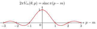
Figure 1: The Wigner function $V_{m}(\theta,p)$ - Eq. (109) - for the basis function $e_{m}(\varphi)$

The Wigner function (109) is independent of $\theta$ and can become negative as a function of $p$, e.g. in the interval $\pm(p-m)\in(1,2)$. So a Wigner function on $S^{1}\times\mathbb{R}$ can have negative values, too, like in the $(q,p)$ case: The Wigner function (phase space density) $W_{n}(q,p)$ for the $n$-th energy level of the quantized harmonic oscillator has the value $\lambda(-1)^{n},\,\lambda>0,$ at $(q=0,p=0)$ sch . In the $(q,p)$ case negativity of Wigner functions on certain subsets of the classical phase space is interpreted as a consequence of quantum effects. The same interpretation applies to the Wigner function here: Whereas the classical angular momentum $p$ is continuous its quantized counterpart is discrete. This is reflected by the properties of the Wigner function (109). The difference between the $(q,p)$ case and the $(\theta,p)$ one is that in the former case the basic variables $q$ and $p$ in general remain continuous in the quantum theory, too, whereas in the latter the basic angular momentum variable $p$ becomes discontinuous.

The integrals (82) - (85) become trivial here:

$$\int_{-\infty}^{\infty}dp\,V_{m}(\theta,p) = \frac{1}{2\pi}$$ (110)

$$\int_{-\pi}^{\pi}d\theta\,V_{m}(\theta,p) = \operatorname{sinc}\pi(p-m)$$

$$= \omega_{m}(p)\,,$$

$$\int_{-\infty}^{\infty}dp\,\omega_{m}(p)\,\operatorname{sinc}(p-m) = |c_{m}|^{2}=1\,,$$ (112)

$$\int_{-\infty}^{\infty}dp\int_{-\pi}^{\pi}d\theta\,V_{m}(\theta,p) = 1.$$ (113)

IV.3.2 Wigner functions of simple “cat” states

The eigenstates $e_{+1}(\varphi)$ and $e_{-1}(\varphi)$ of the angular momentum operator $L$ with eigenvalues $m=\pm 1$ are the first excited states of a rotator with the simple Hamiltonian $H=\varepsilon\,L^{2}$, both with the same energy eigenvalue $\varepsilon$. They represent, however, two different types of rotations: clockwise and counterclockwise. The Wigner functions of their simple superpositions (“cat” states)

$$f_{+1,-1:+}(\varphi) = \frac{1}{\sqrt{2}}[e_{m=1}(\varphi)+e_{m=-1}(\varphi)]$$

$$= \frac{1}{\sqrt{2}}[e^{i\varphi}+e^{-i\varphi}]=\sqrt{2}\cos\varphi,$$

$$|f_{+1,-1:+}(\varphi)|^{2} = 1+\cos 2\varphi=2\cos^{2}\varphi,$$ (115)

$$f_{+1,-1:-}(\varphi) = \frac{1}{\sqrt{2}}[e_{m=1}(\varphi)-e_{m=-1}(\varphi)]$$

$$= \frac{1}{\sqrt{2}}[e^{i\varphi}-e^{-i\varphi}]=i\sqrt{2}\sin\varphi,$$

$$|f_{+1,-1:-}(\varphi)|^{2} = 1-\cos 2\varphi=2\sin^{2}\varphi,$$ (117)

show in an interesting manner the influence of the interference or entanglement term $\cos 2\varphi$ for the corresponding phase space densities $V_{f_{\pm}}(\theta,p)$ (in the following we write $f_{+}(\varphi)$ for $f_{+1,-1:+}(\varphi)$).

Inserting $f_{+}(\varphi)$ into Eq. (IV.1) we get its Wigner function

$$2\pi V_{f_{+}}(\theta,p)=\cos 2\theta\operatorname{sinc}\pi p+\frac{1}{2}[\operatorname{sinc}\pi(p+1)+\operatorname{sinc}\pi(p-1)].$$ (118)

The integrals (82) - (85) now take the form

$$\int_{-\infty}^{\infty}dp\,V_{f_{+}}(\theta,p) = \frac{1}{2\pi}(\cos 2\theta+1)\,,$$ (119)

$$\int_{-\pi}^{\pi}d\theta\,V_{f_{+}}(\theta,p) = \frac{1}{2}[\operatorname{sinc}\pi(p+1)+\operatorname{sinc}\pi(p-1)]$$ (120)

$$\equiv \omega_{f_{+}}(p)\,,$$

$$\int_{-\infty}^{\infty}dp\,\omega_{f_{+}}(p)\,\operatorname{sinc}\pi(p+1) = |c_{-1}|^{2}=\frac{1}{2}\,,$$ (121)

$$\int_{-\infty}^{\infty}dp\,\omega_{f_{+}}(p)\,\operatorname{sinc}\pi(p-1) = |c_{+1}|^{2}=\frac{1}{2}\,,$$ (122)

$$\int_{-\infty}^{\infty}dp\int_{-\pi}^{\pi}d\theta\,V_{f_{+}}(\theta,p) = 1.$$ (123)

The $\theta$-dependent term in Eq. (118) represents the interference or entanglement part of the probability density (115). Graphs of the function (118) – shown in FIG. 2 –, parametrized by different angles $\theta\in[-\pi,+\pi]$ demonstrate the strong influence that interference term has on the phase space function $V_{f_{+}}(\theta,p)$.

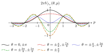
Figure 2: Graphs of the Wigner function $2\pi V_{f_{+}}(\theta,p)=\cos 2\theta\operatorname{sinc}\pi p+\frac{1}{2}[\operatorname{sinc}\pi(p+1)+\operatorname{sinc}\pi(p-1)]$ for the “cat” state $f_{+}(\varphi)=\frac{1}{\sqrt{2}}[e_{m=1}(\varphi)+e_{m=-1}(\varphi)]$ as a continuous function of the classical angular momentum $p$ for different discrete values of the phase space angle $\theta\in[-\pi,+\pi]$. Notice the special cases $2\pi V_{f_{+}}(\theta,p=0)=\cos 2\theta$ and $2\pi V_{f_{+}}(\theta,p=\pm 1)=1/2$ .

The Wigner function $V_{f_{-}}$ for the state (IV.3.2) is

$$2\pi V_{f_{-}}(\theta,p) = -\cos 2\theta\operatorname{sinc}\pi p$$

$$+\frac{1}{2}[\operatorname{sinc}\pi(p+1)+\operatorname{sinc}\pi(p-1)].$$

and can be discussed in the same way as that of $f_{+}$.

Both, $f_{+}(\varphi)$ and $f_{-}(\varphi)$ are special cases of $f_{\alpha}(\varphi)=1/\sqrt{2}(e^{i\varphi}+e^{-i\alpha}\,e^{-i\varphi})$, which leads to the same Wigner function as in Eq. (118), with $2\theta$ replaced by $2\theta+\alpha$.

IV.3.3 Minimal uncertainty states

The following example of a special state is taken from Sec. III of Ref. Kastrup (2006) (for a related later discussion see Ref. Řeháček et al. (2008)): If $A$ and $B$ are two (non-commuting) self-adjoint operators and if the state $\psi$ belongs to their common domain of definition, then the general “uncertainty relation” Robertson (1929); Schrödinger (1930); Jackiw (1968)

$$(\Delta A)^{2}_{\psi}(\Delta B)^{2}_{\psi}\geq|\langle S_{\psi}(A,B)\rangle_{\psi}|^{2}+\frac{1}{4}|\langle[A,B]\rangle_{\psi}|^{2}\,,$$ (125)

holds, where

$$(\Delta A)^{2}_{\psi} = \langle(A-\langle A\rangle_{\psi})^{2}\rangle_{\psi}\,,\langle A\rangle_{\psi}=(\psi,A\psi),~{}~{}~{}~{}$$ (126)

$$S_{\psi}(A,B) = \frac{1}{2}(AB+BA)-\langle A\rangle_{\psi}\langle B\rangle_{\psi}.$$ (127)

Of special interest are those states $\psi=\psi_{e}$ for which the inequality (125) becomes an equality. That equality holds iff $\psi_{e}$ obeys the linear dependence equation

$$(B-\langle B\rangle_{\psi_{e}})\psi_{e}=\sigma\,(A-\langle A\rangle_{\psi_{e}})\psi_{e}\,,~{}\sigma=\gamma+is\,,$$ (128)

where the given real parameters $\gamma$ and $s$ determine the following statistical quantities:

$$\frac{\langle S_{\psi_{e}}(A,B)\rangle_{\psi_{e}}}{(\Delta A)^{2}_{\psi_{e}}} = \gamma\,,$$ (129)

$$\frac{1}{2i}\frac{\langle[A,B]\rangle_{\psi_{e}}}{(\Delta A)^{2}_{\psi_{e}}} = s\,,$$ (130)

$$\frac{(\Delta B)^{2}_{\psi_{e}}}{(\Delta A)^{2}_{\psi_{e}}} = |\sigma|=\sqrt{\gamma^{2}+s^{2}}\,.$$ (131)

In the usual case $A=Q,B=P$ the solutions $\psi_{e}$ of Eq. (128) are Gaussian wave packets (coherent states), for which $\gamma=0$:

$$\psi_{e}(x) = (s/\pi)^{1/4}e^{\displaystyle-(s/2)(x-x_{e})^{2}}e^{\displaystyle ip_{e}x},\,s>0,~{}~{}~{}$$

$$x_{e}=\langle Q\rangle_{\psi_{e}},\,p_{e}=\langle P\rangle_{\psi_{e}}\,.$$

In our case we take $A=S=\sin\varphi,\,\langle S\rangle_{\psi_{e}}=0$ and $B=L=(1/i)\partial_{\varphi}$ (in Ref. Kastrup (2006) Sec. III starts with $A=C=\cos\varphi$, but $A=\sin\varphi$ is closer to the standard von Mises statistical distribution Forbes et al. (2011); Mardia and Jupp (2000)). Assuming here $\gamma=0$, too, the choice $A=\sin\varphi$ and $B=L$ yields the following normalized solution of Eq. (128):

$$\psi_{e}(\varphi) = \frac{1}{\sqrt{I_{0}(2s)}}e^{\displaystyle ip_{e}\varphi+s\cos\varphi}\,,\,s>0\,,$$ (133)

$$|\psi_{e}(\varphi)|^{2} = \frac{e^{\displaystyle 2s\cos\varphi}}{I_{0}(2s)}\,,$$ (134)

$$p_{e} = \langle L\rangle_{\psi_{e}}\,,$$ (135)

$$\langle S\rangle_{\psi_{e}} = 0\,,$$ (136)

$$\langle C\rangle_{\psi_{e}} = \frac{I_{1}(2s)}{I_{0}(2s)}\,.$$ (137)

If one would allow for $S_{e}=\langle S\rangle_{\psi_{e}}\neq 0$ in Eq. (128) the solution (133) would include a non-periodic factor $\exp(s\,S_{e}\varphi)$ which cannot be incorporated into any Hilbert space with a scalar product (22) and a basis (23). Similarly the solution (IV.3.3) of Eq. (128) is not square-integrable on the real line for $s<0$.

The functions $I_{n}(x)$ are modified Bessel functions (for more details which we do not need here see Ref. Kastrup (2006)). The following integral representation for $n\in\mathbb{Z}$ has been und will be used Watson (1966):

$$I_{n}(z)=\frac{1}{2\pi}\int_{-\pi}^{\pi}d\phi\,e^{\displaystyle z\cos\phi+in\phi}=I_{-n}(z)\,.$$ (138)

$I_{n}(z)$ is real for real $z$ and $I_{n}(-z)=(-1)^{n}I_{n}(z)$.

For the shapes of the distribution (134) for different values of $s$ see Fig. 3.1 of Ref. Mardia and Jupp (2000).

As

$$\psi_{e}(\varphi+2\pi)=e^{\displaystyle i2\pi p_{e}}\psi_{e}(\varphi)\,,$$ (139)

the function (133) is generally not periodic, because $p_{e}$ can be any real number. However its treatment can be reduced to the case discussed in the context of Eqs. (23) and (24): we decompose the real number $p_{e}$ uniquely into an integer $n_{e}$ and a fractional rest:

$$p_{e}=n_{e}+\delta\,,~{}\delta\in[0,1)\,,$$ (140)

so that

$$\psi_{e}(\varphi)=\frac{1}{\sqrt{I_{0}(2s)}}e^{\displaystyle i(n_{e}+\delta)\varphi+s\cos\varphi}\,.$$ (141)

This yields the expansion coefficients

$$c_{m}=(e_{m,\delta},\psi_{e})$$

$$= \frac{1}{\sqrt{I_{0}(2s)}}\int_{-\pi}^{\pi}\frac{d\varphi}{2\pi}e^{\displaystyle-i(m-n_{e})\varphi+s\cos\varphi}$$

$$= \frac{1}{\sqrt{I_{0}(2s)}}I_{m-n_{e}}(s)\,.$$

In order to calculate the Wigner function of the state (133) we have to use the Wigner-Moyal matrix (173) of the next Section: We then get

$$V^{[\delta]}_{\psi_{e}}(\theta,p)=\sum_{m.n\in\mathbb{Z}}c^{\ast}_{m}V^{[\delta]}_{mn}(\theta,p)c_{n}\,.$$ (143)

Using for $c_{m}$, $c_{n}$ and $V^{[\delta]}_{mn}(\theta,p)$ the integral representations (IV.3.3) and (173) below and observing the relation (44) (twice) yields the integral representation

$$~{}~{}~{}V^{[\delta]}_{\psi_{e}}(\theta,p)=$$

$$=\frac{1}{(2\pi)^{2}I_{0}(2s)}\int_{-\pi}^{\pi}d\vartheta\,e^{\displaystyle-i(p-p_{e})\vartheta+2s\cos\theta\cos(\vartheta/2)}$$

$$=\frac{1}{2\pi^{2}I_{0}(2s)}\int_{0}^{\pi}d\vartheta\,\cos[(p-p_{e})\vartheta]e^{\displaystyle 2s\cos\theta\cos(\vartheta/2)},$$

$$~{}~{}~{}p_{e}=n_{e}+\delta\,.$$

We drop the label $[\delta]$ of $V^{[\delta]}_{\psi_{e}}(\theta,p)$ in the following.

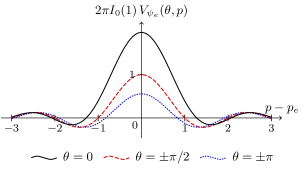
Figure 3: Graphs of the Wigner function (IV.3.3) for the state (133) with $s=1/2$. The curves show $2\pi I_{0}(1)V_{\psi_{e}}(\theta,p)$ for $\theta=0,\,\pm\pi/2,\,\pm\pi$ as a function of $p-p_{e}$. Numerically: $I_{0}(1)=1.2661$ wa (2).

For the values $\theta=\pm\pi/2$ we have

$$V_{\psi_{e}}(\theta=\pm\pi/2,p)=\frac{1}{2\pi I_{0}(2s)}\,\operatorname{sinc}\pi(p-p_{e})\,.$$ (145)

The variables $p$ and $p_{e}$ are to be treated independently ($p_{e}$ is the given“observable” $\langle L\rangle_{\psi_{e}}$, $p$ a phase space variable). The curves in FIG. 3 have their main maximum for $p=p_{e}$.

The Wigner function (IV.3.3) indeed obeys the general relations (82) - (85) explicitly:

Integrating Eq. (IV.3.3) over $p$ gives a delta function $\delta(\vartheta)$ which makes the $\vartheta$-integral trivial. The result is the expected marginal density (134):

$$\int_{-\infty}^{\infty}dp\,V_{\psi_{e}}(\theta,p)=\frac{1}{2\pi I_{0}(2s)}e^{\displaystyle 2s\cos\theta}=\frac{1}{2\pi}|\psi_{e}(\theta)|^{2}.$$ (146)

The $\theta$-integration and the ensuing determination of $|c_{m}|^{2}$ are slightly more subtle:

$$\int_{-\pi}^{\pi}d\theta\,V_{\psi_{e}}(\theta,p)=\omega_{\psi_{e}}(p)=$$

$$=\frac{1}{2\pi I_{0}(2s)}\,\int_{-\pi}^{\pi}d\vartheta\,e^{\displaystyle-i(p-p_{e})\vartheta}I_{0}(2s\cos(\vartheta/2)$$

$$=\frac{1}{\pi I_{0}(2s)}\,\int_{0}^{\pi}d\vartheta\,\cos[(p-p_{e})\vartheta]I_{0}(2s\cos(\vartheta/2),$$

where again the relation (138) has been used.

In order to extract from $\omega_{\psi_{e}}$ the marginal probabilities $|c_{m}|^{2}$ - according to Eq. (84) - we have to multiply $\omega_{\psi_{e}}(p)$ with $\operatorname{sinc}\pi(p-m-\delta)$ and integrate over $p$:

$$\int_{-\infty}^{\infty}dp\,\omega_{\psi_{e}}(p)\operatorname{sinc}\pi(p-m-\delta)\,.$$ (148)

Inserting

$$\operatorname{sinc}\pi(p-m-\delta)=\frac{1}{2\pi}\int_{-\pi}^{\pi}d\alpha\,e^{\displaystyle i(p-m-\delta)\alpha}$$ (149)

into Eq. (148) yields a delta function $\delta(\alpha-\vartheta)$ and

$$\frac{1}{2\pi I_{0}(2s)}\int_{-\pi}^{\pi}d\vartheta\,e^{\displaystyle i(m-n_{e})\vartheta}I_{0}(2s\cos(\vartheta/2)$$

$$= \frac{1}{\pi I_{0}(2s)}\int_{0}^{\pi}d\vartheta\,\cos[(m-n_{e})\vartheta]\,I_{0}(2s\cos(\vartheta/2)$$

for the integral (148). As Erdélyi (1954); Gradshteyn and Ryzhik (1965)

$$\int_{-\pi/2}^{\pi/2}d\beta\,\cos(2n\beta)\,I_{0}(2a\cos\beta)=\pi I_{n}^{2}(a)$$ (151)

the integral (148) gives indeed the same probability

$$|c_{m}|^{2}=\frac{1}{I_{0}(2s)}\,|I_{m-n_{e}}(s)|^{2}$$ (152)

as obtained from Eq. (IV.3.3).

IV.3.4 Thermal states

Let simple rotators with the Hamiltonian (75) be in a heat bath of temperature $T$. Then the density matrix (62) has the form

$$\rho = (\lambda_{n}\delta_{mn})\,,~{}\lambda_{n}=\frac{e^{\displaystyle-n^{2}\varepsilon\beta}}{Z(\beta)},$$ (153)

$$\beta = 1/(k_{B}T),$$

$$Z(\beta) = \sum_{n\in\mathbb{Z}}e^{\displaystyle-n^{2}\varepsilon\beta}.$$ (154)

The partition function (154) can be expressed in terms of a $\vartheta$-function the :

$$\vartheta_{3}(z,q=e^{\displaystyle i\pi\tau}) \equiv \vartheta_{3}(z|\tau)=\sum_{n\in\mathbb{Z}}q^{\displaystyle n^{2}}e^{\displaystyle 2niz}$$ (155)

$$= 1+2\sum_{n=1}^{\infty}q^{\displaystyle n^{2}}\cos 2nz$$

$$= \vartheta_{3}(-z,q)\,,$$

$$\Im(\tau)>0\,.$$

The function (155) is an entire function of $z$, real valued for real and imaginary $z$ if $q$ is real. For real $q$ there are also no zeros on the real and imaginary $z$-axis and $\vartheta_{3}(z,q)$ is positive there.

We now can write

$$Z(\beta) = \vartheta_{3}(z=0,q=e^{\displaystyle-\varepsilon\beta})$$

$$= \vartheta_{3}(z=0|\tau=i\varepsilon\beta/\pi).$$

For $\varepsilon\beta\gg 1$ (low temperatures) the first order in $q$ in the series (IV.3.4) gives a reasonable approximation:

$$Z(\beta)\approx 1+2e^{\displaystyle-\varepsilon\beta},~{}~{}1/Z(\beta)\approx 1-2e^{\displaystyle-\varepsilon\beta},~{}\varepsilon\beta\gg 1.$$ (158)

(For $\varepsilon\approx O(\mbox{1 eV})$ and $T\approx 300^{\circ}$K one has $\varepsilon\,\beta\approx 40$). A corresponding high-temperature approximation can be obtained with the help of Jacobi’s famous identity

$$\vartheta_{3}(z|\tau)=(-i\tau)^{\displaystyle-1/2}e^{\displaystyle-iz^{2}/(\pi\tau)}\vartheta_{3}(z/\tau|-1/\tau).$$ (159)

It yields

$$Z(\beta)=\left(\frac{\pi}{\varepsilon\beta}\right)^{1/2}\vartheta_{3}(z=0,q=e^{\displaystyle-\pi^{2}/(\varepsilon\beta)}),$$ (160)

which for $\varepsilon\beta\ll 1$ provides the approximation

$$Z(\beta) \approx \left(\frac{\pi}{\varepsilon\beta}\right)^{1/2}(1+2e^{\displaystyle-\pi^{2}/(\varepsilon\beta)}),~{}\varepsilon\beta\ll 1\,,~{}~{}~{}~{}~{}$$ (161)

$$1/Z(\beta) \approx \left(\frac{\varepsilon\beta}{\pi}\right)^{1/2}(1-2e^{\displaystyle-\pi^{2}/(\varepsilon\beta)}).$$ (162)

Due to $\varepsilon\beta\ll 1$ and the exponent $\pi^{2}$ in $q=\exp(-\pi^{2}/(\varepsilon\beta))$ this $q$ is negligible compared to $1$. For the Wigner function (93) we get - according to Eq. (63) - :

$$V_{\rho}(\theta,p) = \operatorname{tr}(\rho\cdot V(\theta,p))$$

$$= \frac{1}{2\pi\,Z(\beta)}\sum_{n\in\mathbb{Z}}e^{\displaystyle-n^{2}\varepsilon\beta}\operatorname{sinc}\pi(p-n)$$

$$= \frac{1}{(2\pi)^{2}\,Z(\beta)}\int_{-\pi}^{\pi}d\alpha\,e^{\displaystyle-ip\alpha}\sum_{n\in\mathbb{Z}}e^{\displaystyle-n^{2}\varepsilon\beta}e^{\displaystyle in\alpha}.$$

This result obviously can be expressed in terms of the $\vartheta$-function (155), too:

$$V_{\rho}(\theta,p) = \operatorname{tr}(\rho\cdot V(\theta,p))$$

$$= \frac{1}{(2\pi)^{2}\,Z(\beta)}\int_{-\pi}^{\pi}d\alpha\,e^{\displaystyle-ip\alpha}\vartheta_{3}(\alpha/2,q=e^{\displaystyle-\varepsilon\beta})$$

$$= \frac{1}{2\pi^{2}\,Z(\beta)}\int_{0}^{\pi}d\alpha\,\cos p\alpha\,\vartheta_{3}(\alpha/2,q=e^{\displaystyle-\varepsilon\beta}).$$

Integrating Eq. (IV.3.4), or (IV.3.4) respectively, over $\theta$ gives a factor $2\pi$, integrating in addition over $p$ gives 1. Multiplying equation (IV.3.4) by $\operatorname{sinc}\pi(p-m)$, integrating over $p$ and using the relation (54) gives the density matrix elements $\lambda_{n}$ of Eq. (153), multplied by $1/(2\pi)$.

In order to get some more insights into the properties of the Wigner function (IV.3.4) it helps to look at its low- and high-temperature limits mentioned above:

In the low-temperature limit $\varepsilon\beta\gg 1$ we have for $\vartheta_{3}(\alpha/2,q=\exp(-\varepsilon\beta))$ in first order of $q$:

$$\vartheta_{3}(\alpha/2,q=e^{\displaystyle-\varepsilon\beta})\approx 1+2e^{\displaystyle-\varepsilon\beta}\cos\alpha.$$ (165)

Inserting this into the integral (IV.3.4), observing that pru

$$\int_{0}^{\pi}d\alpha\,\cos\alpha\,\cos p\alpha=-\frac{\pi}{2}\,\operatorname{sinc}\pi p\left(\frac{p}{p+1}+\frac{p}{p-1}\right)$$ (166)

and using the approximation (158) yields

$$V^{(l)}_{\rho}(\theta,p)=\frac{1}{2\pi}\operatorname{sinc}\pi p\left[1-e^{\displaystyle-\varepsilon\beta}\left(2+\frac{p}{p+1}+\frac{p}{p-1}\right)\right].$$ (167)

This low-temperature approximation of $V_{\rho}(\theta,p)$ is dominated by the $\operatorname{sinc}\pi p$ function in the neighbourhood of $p=0$. That function also compensates the poles at $p=\pm 1$: For, e.g. $p=1+\epsilon$ we have $\lim_{\epsilon\to 0}\operatorname{sinc}\pi(1+\epsilon)/\epsilon=-1$.

Thus, at very low temperatures the wave function (167) dominantly describes thermally very small angular momenta, as expected!

For the high-temperature approximation we use the relation

$$\vartheta_{3}(\alpha/2,q=e^{\displaystyle-\varepsilon\beta})$$

$$=\left(\frac{\pi}{\varepsilon\beta}\right)^{1/2}e^{\displaystyle-\alpha^{2}/(4\varepsilon\beta)}\vartheta_{3}\left(z=\frac{i\pi\alpha}{2\varepsilon\beta},q=e^{\displaystyle-\pi^{2}/(\varepsilon\beta)}\right),$$

which follows from Jacobi’s identity (159).

If the functions $Z(\beta)$ and $\vartheta_{3}$ of Eqs. (160) and (IV.3.4) are inserted in Eq. (IV.3.4) their common prefactor drops out. We then get for $V_{\rho}$ the high-temperature approximation

$$V^{(h)}_{\rho}(\theta,p)=\frac{1}{2\pi^{2}}\int_{0}^{\pi}d\alpha\,\cos p\alpha\,e^{\displaystyle-\alpha^{2}/(4\varepsilon\beta)}.$$ (169)

As $\varepsilon\beta\ll 1$ the Gaussian under the integral is short-ranged and therefore we can extend the upper limit of the integral from $+\pi$ to $+\infty$ and obtain gra

$$V^{(h)}_{\rho}(\theta,p)\approx\frac{\sqrt{\pi\varepsilon\beta}}{2\pi^{2}}e^{\displaystyle-\varepsilon\beta\,p^{2}}.$$ (170)

Thus, at high temperatures the Wigner function (IV.3.4) becomes a Boltzmann distribution for the classical angular momenta $p$! (Note that $\varepsilon p^{2}$ is the classical counterpart to the quantum mechanical Hamiltonian (75).) Integrating this $V^{(h)}_{\rho}$ over $p$ gives

$$\int_{-\infty}^{\infty}dpV^{(h)}_{\rho}(\theta,p)=\frac{1}{2\pi}.$$ (171)

The denominator $2\pi$ on the right-hand side is cancelled by the final (trivial) integration over $\theta$.

V The cases $\mathbf{\delta\neq 0}$ and $\mathbf{\hbar\neq 1}$

V.1 $\mathbf{\delta\neq 0}$

In Ref. Kastrup (2006) a number of physical examples were mentioned for which the parameter $\delta$ of Eqs. (22) - (24) is nonvanishing. Another example with $\delta\neq 0$ was discussed in the last Subsection. It is, therefore, of interest to indicate the main changes of the principle formulae in Section III if $\delta\neq 0$:

Going through the arguments of Subsection II.B, above, now using the basis functions (23), we get instead of Eqs. (35) and (35)

$$V^{[\delta]}_{mn}(\theta,p)$$ (173)

$$=\frac{1}{(2\pi)^{2}}\,e^{\displaystyle i(n-m)\theta}\int_{-\pi}^{\pi}d\vartheta\,e^{\displaystyle i[(n+m+2\delta)/2-p]\vartheta}$$

$$=\frac{1}{2\pi}\,e^{\displaystyle i(n-m)\theta}\,\operatorname{sinc}\pi[p-(m+n+2\delta)/2]\,.$$

The relations (36) - (40) now take the form

$$\int_{-\infty}^{\infty}dp\,V^{[\delta]}_{mn}(\theta,p)=\frac{1}{2\pi}\,e^{\displaystyle i(n-m)\theta}\,,$$ (174)

$$\int_{-\pi}^{\pi}d\theta\,V^{[\delta]}_{mn}(\theta,p)=\operatorname{sinc}\pi(p-m-\delta)\,\delta_{mn}\,,$$ (175)

$$\int_{-\pi}^{\pi}d\theta\int_{-\infty}^{\infty}dp\,V^{[\delta]}_{mn}(\theta,p)=\delta_{mn},\,$$ (176)

$$\,\,\operatorname{tr}(V^{[\delta]}_{mn})=\frac{1}{2\pi}\sum_{n\in\mathbb{Z}}\operatorname{sinc}\pi(p-n-\delta)=\frac{1}{2\pi},$$ (177)

$$\int_{-\pi}^{\pi}d\theta\int_{-\infty}^{\infty}dp\,V^{[\delta]\ast}_{kl}(\theta,p)\,V^{[\delta]}_{mn}(\theta,p)=\frac{1}{2\pi}\delta_{km}\delta_{ln}\,.$$ (178)

Using expansions (24) we get instead of Eq. (49)

$$V^{[\delta]}_{\psi_{2}\psi_{1}}(\theta,p)=\sum_{m,n\in\mathbb{Z}}c_{m}^{(2)\ast}V^{[\delta]}_{mn}(\theta,p)c_{n}^{(1)}$$ (179)

$$=\frac{1}{(2\pi)^{2}}\int_{-\pi}^{\pi}d\vartheta\,e^{\displaystyle-ip\vartheta}\psi_{2}^{[\delta]\ast}(\theta-\vartheta/2)\,\psi^{[\delta]}_{1}(\theta+\vartheta/2)\,$$

$$=(\psi^{[\delta]}_{2},V(\theta,p)\psi^{[\delta]}_{1})\,$$

The relation (54) is to be replaced by

$$\int_{-\infty}^{\infty}dp\,\operatorname{sinc}\pi(m+\delta-p)\,\operatorname{sinc}\pi(n+\delta-p)=\delta_{mn}\,.$$ (180)

It is apparently rather obvious how one has to proceed if one passes from a Hilbert space with $\delta=0$ to one with $\delta\neq 0$, e.g. in Section IV, Subsections A and B.

V.2 $\hbar\neq 1$

In the Sections above we have put $\hbar=1$. To make $\hbar$ explicit again in all the formulae is easier here than in the $(q,p)$ case, because the basic variable $\theta$ is dimensionless and only the canonically conjugate angular momentum $p$ which has the dimension [action] has to be rescaled:

In order to reintroduce $\hbar$ into the above formulae the following two replacements are necessary: First the angular momentum operator $L$ of Eq. (25) has to be rescaled:

$$L=\frac{1}{i}\partial_{\varphi}\to\hat{L}=\frac{\hbar}{i}\partial_{\varphi}\,.$$ (181)

Notice that the basis functions (23) remain unchanged and are now eigenfunctions of $\hat{L}$ with eigenvalues $\hbar\,n$.

In addition the classical phase space variable $p$, which we have treated as dimensionless above, has to be replaced by $p/\hbar$ if $p$ is now interpreted as a variable with the dimension [action].

As an example consider the $\operatorname{sinc}$ function of Eq. (1):

$$\operatorname{sinc}\pi(p-m) \to \operatorname{sinc}[\pi(p-\hbar\,m)/\hbar]$$

$$= \hbar\,\frac{\sin[\pi(p-m\,\hbar)/\hbar]}{\pi(p-\hbar\,m)}.$$

Thus, the $\operatorname{sinc}$-function (V.2) is dimensionless. So are the matrix $V(\theta,p)$ and the wave functions (48). As

$$\lim_{\epsilon\to 0}\frac{\sin(\pi x/\epsilon)}{\pi x}=\delta(x)\,,$$ (183)

the associated classical limit of the rescaled expression (V.2) can be obtained as

$$\lim_{\hbar\to 0}\frac{1}{\hbar}\operatorname{sinc}[\pi(p-\hbar\,m)/\hbar]=\delta(p-\hbar\,m)\,,\,\,\hbar\,m=\text{const.}\,.$$ (184)

In Subsection III.C. the time derivatives $\partial_{t}$ have to be replaced by $\hbar\,\partial_{t}$.

VI remarks

VI.1 Dirac notation

Throughout the whole text above I have avoided the use of the widespread Dirac notion of ”bra”, ”ket” etc. for describing quantum mechanical states and operators. The reason being (see, e.g. Ref. Kastrup (2006)) that there is no mathematically well-defined angle operator $\hat{\varphi}$ with eigenfunctions $|\varphi\rangle$ such that

$$\hat{\varphi}|\varphi\rangle=\varphi\,|\varphi\rangle\,.$$ (185)

The use of such mathematically non-existent objects might be helpful heuristically if one is appropriately careful: Here the formal objects $|\varphi\rangle$ only make sense in the combination

$$\langle\varphi|n\rangle=e^{\displaystyle in\varphi}=e_{n}(\varphi)\,,~{}~{}L|n\rangle=n|n\rangle\,,$$ (186)

where $L$ is the well-defined angular momentum operator. Armed with this mental reservation one may write for the operator $V$ of Eq. (35)

$$\tilde{V}(\theta,p)=\frac{1}{(2\pi)^{2}}\int_{-\pi}^{\pi}d\vartheta\,e^{\displaystyle-ip\vartheta}|\theta-\vartheta/2\rangle\langle\theta+\vartheta/2|\,,$$ (187)

the matrix elements $\tilde{V}_{mn}=\langle m|\tilde{V}|n\rangle$ of which are the same as those in Eq. (35).

The Wigner function in Eq. (IV.1) may be written as

$$V_{\psi}(\theta,p)=\tilde{V}_{\psi}(\theta,p)=\langle\psi|\tilde{V}(\theta,p)|\psi\rangle\,,$$ (188)

where $|\psi\rangle$ is to be considered as an expansion in terms of the eigenstates $|n\rangle$.

Another interesting example is (see Section III.B.)

$$\operatorname{tr}[V(\theta,p)\cdot A] = \operatorname{tr}[\tilde{V}(\theta,p)\cdot A]$$

$$= \frac{1}{(2\pi)^{2}}\int_{-\pi}^{\pi}d\vartheta\,e^{\displaystyle-ip\vartheta}\langle\theta+\vartheta/2|A|\theta-\vartheta/2\rangle\,.$$

Inserting the completeness relations $\sum_{m\in\mathbb{Z}}|m\rangle\langle m|=\mathbf{1}$ and $\sum_{n\in\mathbb{Z}}|n\rangle\langle n|=\mathbf{1}$ before and after the operator $A$ in the last expression leads back to the results of Section III.B.

VI.2 A possible generalisation and some related work

The approach discussed above for phase spaces of the topological type $S^{1}\times\mathbb{R}$ can be generalized, e.g. to a free rigid body in 3 dimensions with one point fixed. Its configuration space can be identified with the group $SO(3)$ chi ; Marsden and Ratiu (2003). Its 2-fold covering $SU(2)$ has the topology of $S^{3}$. The associated phase space $S^{3}\times\mathbb{R}^{3}$ can be quantized in terms of unitary representations of the Euclidean group $E(4)$ ish .

At a late stage of the present investigations I became aware of the work by Leaf Leaf (1968a, b) in which the operator $\Delta(q,p)$ plays a role with respect to the $(q,p)$ Wigner function which corresponds to that of the operator/matrix $V(\theta,p)$ in the discussions above. Leaf’s approach was used by de Groot and Suttorp in their textbook de Groot and Suttorp (1972).

A Wigner-Moyal function on the circle very similar in structure to the one in Eq. (49) above can be found in Refs. Alonso et al. (2003); Mukunda et al. (2005). There, however, the classical angular momentum is treated as discontinuous, contrary to its properties in its classical phase space and its treatment in the present paper!

Finally I am indebted to my son David for providing the figures and for his help with the final LaTeX typewriting.

References

- Wigner (1932) E. Wigner, “On the quantum correction for thermodynamic equilibrium,” Phys. Rev. 40, 749 (1932).
- Hillery et al. (1984) M. Hillery, R. F. O’Connell, M. O. Scully, and E. P. Wigner, “Distribution functions in physics: Fundamentals,” Phys. Rep. 106, 121 (1984).
- Leonhardt (1997) U. Leonhardt, Measuring the Quantum State of Light, Cambridge Studies in Modern Optics, Vol. 22 (Cambridge University Press, Cambridge, UK, 1997).
- Schleich (2001) W. P. Schleich, Quantum Optics in Phase Space (Wiley-VCH, Berlin, 2001).
- Römer (2009) H. Römer, Theoretical Optics: An Introduction, 2nd ed. (Wiley-VCH, Weinheim, 2009).
- Leonhardt (2010) U. Leonhardt, Essential Quantum Optics: From Quantum Measurements to Black Holes (Cambridge University Press, Cambridge, UK, 2010).
- Agarwal (2013) G. S. Agarwal, Quantum Optics (Cambridge University Press, Cambridge, UK, 2013).
- Gröchenig (2001) K. Gröchenig, Foundations of Time-Frequency Analysis, Applied and Numerical Harmonic Analysis (Springer Science+Business Media, New York, 2001).
- Cohen (2013) L. Cohen, The Weyl Operator and its Generalization, Pseudo-Differential Operators, Theory and Applications, Vol. 9 (Birkhäuser, Springer, Basel, 2013).
- Kastrup (2006) H. A. Kastrup, “Quantization of the canonically conjugate pair angle and orbital angular momentum,” Phys. Rev. A 73, 052104 (2006), here Appendix A. Compared to this Ref. Kastrup (2006) the present follow-up paper has some minor changes of notations.
- Berry (1977) M. V. Berry, “Semi-classical mechanics in phase space: A study of wigner’s function,” Phil. Trans. Roy. Soc. London A 287, 237 (1977).
- Mukunda (1979) N. Mukunda, “Wigner distribution for angle coordinates in quantum mechanics,” Am. J. Phys. 47, 182 (1979).
- Rigas et al. (2011) I. Rigas, L. L. Sánchez-Soto, A. B. Klimov, J. Řeháček, and Z. Hradil, “Orbital angular momentum in phase space,” Ann. Phys. (NY) 326, 426 (2011).
- Przanowski et al. (2014) M. Przanowski, P. Brzykcy, and J. Tosiek, “From the Weyl quantization of a particle on the circle to number–phase Wigner functions,” Ann. Phys. (NY) 351, 919 (2014).
- Mukunda et al. (2005) N. Mukunda, G. Marmo, A. Zampini, S. Chaturvedi, and R. Simon, “Wigner-Weyl isomorphism for quantum mechanics on Lie groups,” J. Math. Phys. 46, 012106 (2005).
- Fronsdal (1979) C. Fronsdal, “Some ideas about quantization,” Rep. Math. Phys. 15, 111 (1979).
- Gadella et al. (1991) M. Gadella, M. A. Martin, L. M. Nieto, and M. A. del Olmo, “The Stratonovich–Weyl correspondence for one-dimensional kinematical groups,” J. Math. Phys. 32, 1182 (1991).
- Arratia and del Olmo (1997) O. Arratia and M. A. del Olmo, “Moyal quantization on the cylinder,” Rep. Math. Phys. 40, 149 (1997).
- Isham (1984) C. J. Isham, “Topological and global aspects of quantum theory,” in Relativity, Groups and Topology II, Les Houches Session XL, 1983, edited by B. S. DeWitt and R. Stora (North Holland, Amsterdam, 1984) pp. 1059 – 1290, here especially pp. 1170–1176, 1224–1226.
- Wolf (1996) K. B. Wolf, “Wigner distribution function for paraxial polychromatic optics,” Opt. Comm. 132, 343 (1996).
- Nieto et al. (1998) L. M. Nieto, N. M. Atakishiyev, S. M. Chumakov, and K. B. Wolf, “Wigner distribution function for Euclidean systems,” J. Phys. A: Math. Gen. 31, 3875 (1998).
- Ali et al. (2000) S. T. Ali, N. M. Atakishiyev, S. M. Chumakov, and K. B. Wolf, “The Wigner function for general Lie groups and the wavelet transform,” Ann. Henri Poincaré 1, 685 (2000).
- Moyal (1949) J. E. Moyal, “Quantum mechanics as a statistical theory,” Proc. Cambridge Philos. Soc. 45, 99 (1949).
- Folland (1989) G. B. Folland, Harmonic Analysis in Phase Space, The Annals of Mathematics Studies, Vol. 122 (Princeton University Press, Princeton, NJ, 1989) Chs. 1 and 2.
- de Gosson (2006) M. de Gosson, Symplectic Geometry and Quantum Mechanics, Operator Theory: Advances and Applications, Vol. 166 (Birkhäuser, Basel, 2006) Parts II and III.
- Whittaker (1915) E. T. Whittaker, “On the functions which are represented by the expansions of the interpolation-theory,” Proc. Roy. Soc. Edinburgh 35, 181 (1915).
- McNamee et al. (1971) J. McNamee, F. Stenger, and E. L. Whitney, “Whittaker’s cardinal function in retrospect,” Mathematics of Computation 25, 141 (1971).
- Stenger (1981) F. Stenger, “Numerical methods based on Whittaker cardinal, or sinc functions,” SIAM Rev. 23, 165 (1981).
- Butzer (1983) P. L. Butzer, “A survey of the Whittaker-Shannon sampling theorem and some of its extensions,” J. Mathem. Research and Exposition (now: … and Application) 3, 185 (1983), publ. by Dalian Univ. of Technology and China Soc. for Industrial and Appl. Mathem.; journal available on the web.
- Higgins (1985) J. R. Higgins, “Five short stories about the cardinal series,” Bull. (N.S.) Amer. Math. Soc. 12, 45 (1985).
- Stenger (1993) Frank Stenger, Numerical Methods Based on Sinc and Analytic Functions, Springer Series in Computational Mathematics, Vol. 20 (Springer-Verlag, New York etc., 1993).
- Stenger (2011) F. Stenger, Handbook of Sinc Numerical Methods, Chapman & Hall/CRC Numerical Analysis and Scientific Computing (CRC Press Taylor & Francis Group, Boca Raton, FL, 2011).
- Vetterli et al. (2014) M. Vetterli, J. Kovačević, and V. K. Goyal, Foundations of Signal Processing (Cambridge University Press, Cambridge, UK, 2014).
- Eldar (2015) Y. C. Eldar, Sampling Theory (Cambridge University Press, Cambridge, UK, 2015).
- Louisell (1963) W. H. Louisell, “Amplitude and phase uncertainty relations,” Phys. Lett. 7, 60 (1963).
- Mackey (1963) G. W. Mackey, The Mathematical Foundations of Quantum Mechanics (W.A. Benjamin, Inc., New York, 1963) p. 103.
- Vilenkin (1968) N. I. Vilenkin, Special Functions and the Theory of Group Representations, Translations of Mathematical Monographs, Vol. 22 (Amer. Math. Soc., Providence, RI, 1968) Ch. IV.
- Sugiura (1990) M. Sugiura, Unitary Representations and Harmonic Analysis: An Introduction, North-Holland Mathematical Library, Vol. 44 (Elsevier, Amsterdam, 1990) Ch. IV.
- Chirikjian and Kyatkin (2000) G. S. Chirikjian and A. B. Kyatkin, Engineering Applications of Noncommutative Harmonic Analysis, with Emphasis on Rotation and Motion Groups (CRC Press, Boca Raton, FL, 2000) p. 151, (of general interest for the present paper is especially Ch. 10).
- Whittaker and Watson (1969) E. T. Whittaker and G. N. Watson, A Course of Modern Analysis, 4th ed. (Cambridge University Press, Cambridge, UK, 1969) p. 362.
- Morse and Feshbach (1953) Ph. M. Morse and H. Feshbach, Methods of Theoretical Physics, Vol. I, International Series in Pure and Applied Physics (McGraw-Hill Book Co., Inc., New York, 1953) p. 766, formula (6.3.62).
- Prudnikov et al. (1986) A. P. Prudnikov, Yu. A. Brychkov, and O. I. Marichev, Integrals and Series, Vol. 1 (Gordon and Breach Science Publishers, New York, London etc., 1986) p. 727, formula 13.6.
- de Groot and Suttorp (1972) S. R. de Groot and L. G. Suttorp, Foundations of Electrodynamics (North-Holland, Amsterdam, 1972) Ch. VI (the representation here relies on Refs. Leaf (1968a, b)).
- Hardy (1941) G. H. Hardy, “Notes on special systems of orthogonal functions (IV): The orthogonal functions of Whittaker’s series,” Proc. Cambridge Philos. Soc. 37, 331 (1941), reprinted in Collected Papers of G.H. Hardy, vol. III (Clarendon Press, Oxford, 1969) p. 466.
- Christensen (2008) O. Christensen, Frames and Bases, An Introductory Course, Applied and Numerical Harmonic Analysis (Birkhäuser, Boston, 2008) here Ch. 3.8.
- (46) See, e.g. Ref. Schleich (2001), Ch. 4 or Ref. Agarwal (2013), Chs. 1.7 and 1.8.
- Řeháček et al. (2008) J. Řeháček, Z. Bouchal, R. Čelechovský, Z. Hradil, and L. L. Sánchez-Soto, “Experimental test of uncertainty relations for quantum mechanics on a circle,” Phys. Rev. A , 032110 (2008).
- Robertson (1929) H. P. Robertson, “The uncertainty principle,” Phys. Rev. 34, 163 (1929).
- Schrödinger (1930) E. Schrödinger, “Zum Heisenbergschen Unschärfeprinzip,” Sitzungsber. Preuss. Akad. Wiss., Phys.-math. Klasse 19, 296 (1930), reprinted in E. Schrödinger, Collected Papers, Vol. 3, p. 348 (Österr. Akad. Wiss. and Friedr. Vieweg & Sohn, Braunschweig/Wiesbaden, Vienna, 1984).
- Jackiw (1968) R. Jackiw, “Minimum uncertainty product, number-phase uncertainty product, and coherent states,” J. Math. Phys. 9, 339 (1968).
- Forbes et al. (2011) C. Forbes, M. Evans, and N. Hastings, Statistical Distributions, 4th ed. (John Wiley & Sons, Inc., Hoboken, NJ, USA, 2011) ch. 45.
- Mardia and Jupp (2000) K. V. Mardia and P. E. Jupp, Directional Statistics, Wiley Series in Probability and Statistics (John Wiley & Sons, Ltd, Chichester etc., UK, 2000) especially Subsec. 3.5.4.
- Watson (1966) G. N. Watson, A Treatise on the Theory of Bessel Functions, 2nd ed. (Cambridge University Press, Cambridge, UK, 1966) p. 181, formula (4).
- wa (2) See, e.g. Ref. Watson (1966), p. 698.
- Erdélyi (1954) A. Erdélyi, ed., Tables of Integral Transforms, Vol. I (McGraw-Hill Book Co., Inc., New York etc., 1954) p. 59, formula (61).
- Gradshteyn and Ryzhik (1965) I. S. Gradshteyn and I. M. Ryzhik, Table of Integrals, Series and Products, 4th ed. (Academic Press, New York, 1965) p. 738, formula 6.681, 3.; the number of the formula is the same in later editions.
- (57) For the literature on the functions see Appendix C of Ref. Kastrup (2006).
- (58) Ref. Prudnikov et al. (1986), p. 403, formula 41.
- (59) Ref. Gradshteyn and Ryzhik (1965), p. 480, formula 3.896, 4.
- (60) See, e.g. Ref. Chirikjian and Kyatkin (2000), Chs. 5 and 6.
- Marsden and Ratiu (2003) J. E. Marsden and T. S. Ratiu, Introduction to Mechanics and Symmetry, 2nd ed. (Springer-Verlag, New York, 2003) here Ch. 15.
- (62) Ref. Isham (1984), example 4.9 (p. 1194); For irreducible unitary representations of Euclidean groups see, e.g. Ch. XI of Ref. Vilenkin (1968) and Ch. 10 of Ref. Chirikjian and Kyatkin (2000).
- Leaf (1968a) B. Leaf, “Weyl transformation and the classical limit of quantum mechanics,” J. Math. Phys. 9, 65 (1968a).
- Leaf (1968b) B. Leaf, “Weyl transform in nonrelativistic quantum dynamics,” J. Math. Phys. 9, 769 (1968b).
- Alonso et al. (2003) M. A. Alonso, G. S. Pogosyan, and K. B. Wolf, “Wigner functions for curved spaces. ii. on spheres,” J. Math. Phys. 44, 1472 (2003), here Subsec. IV. A.