Infrared Continuum and Line Evolution of the Equatorial Ring around SN 1987A

Abstract

Spitzer observations of SN 1987A have now spanned more than a decade. Since day $\sim 4,000$, mid-infrared (mid-IR) emission has been dominated by that from shock-heated dust in the equatorial ring (ER). From 6,000 to 8,000 days after the explosion, Spitzer observations included broadband photometry at 3.6 – 24 $\mu$m, and low and moderate resolution spectroscopy at 5 – 35 $\mu$m. Here we present later Spitzer observations, through day 10,377, which include only the broadband measurements at 3.6 and 4.5 $\mu$m. These data show that the 3.6 and 4.5 $\mu$m brightness has clearly begun to fade after day $\sim 8,500$, and no longer tracks the X-ray emission as well as it did at earlier epochs. This can be explained by the destruction of the dust in the ER on time scales shorter than the cooling time for the shocked gas. We find that the evolution of the late time IR emission is also similar to the now fading optical emission. We provide the complete record of the IR emission lines, as seen by Spitzer prior to day 8,000. The past evolution of the gas as seen by the IR emission lines seems largely consistent with the optical emission, although the IR [Fe II] and [Si II] lines show different, peculiar velocity structures.

1. Introduction

SN 1987A presents, thus far, a unique opportunity for the detailed study of the evolution of a supernova into a supernova remnant (see reviews by McCray, 1993, 2007). Its proximity allows the imaging of small scale structure of both the SN ejecta and the circumstellar environment. It also is sufficiently bright that at most wavelengths high S/N observations can be obtained very quickly, even at high spectral resolution. SN 1987A was not a prototypical Type II supernova, exhibiting a subluminous light curve with a late maximum, and having a known blue supergiant progenitor (e.g. Arnett et al., 1989). However, a number of other blue supergiant stars have been found to have similar circumstellar structures (Brandner et al., 1997a, b; Smith, 2007; Smith et al., 2013; Muratore et al., 2015; Gvaramadze et al., 2015).

Shortly after its launch, the Spitzer Space Telescope (Werner et al., 2004; Gehrz et al., 2007) began a long-term campaign of imaging and spectroscopy of SN 1987A at wavelengths from 3.6 – 160 $\mu$m. At the near- and mid-IR wavelengths Spitzer has been able to monitor thermal emission from warm dust in the SN. Despite insufficient angular resolution to resolve detailed structure, this emission has been identified (Bouchet et al., 2006) as arising from dust in the equatorial ring (ER) that was formed by winds during mass loss episodes of the SN progenitor star (or binary system, e.g. Podsiadlowski & Joss, 1989).

Dust is also known to be present in SN 1987A’s ejecta. Photometric and spectroscopic evidence of dust formation in the ejecta began to appear after day $\sim 450$ (Danziger et al., 1989; Suntzeff & Bouchet, 1990). From days 615 – 1,144, mid-IR spectrophotometry by Moseley et al. (1989); Dwek et al. (1992) and Wooden et al. (1993) monitored the emission of the dust directly. However at much later times, the ejecta has cooled and faded, and has been too faint to be detected by Spitzer at mid- or far-IR wavelengths. At present times, the ejecta dust has been detected in the far-IR with larger, more sensitive instruments such as Herschel and ALMA (Matsuura et al., 2011; Lakićević et al., 2012; Kamenetzky et al., 2013; Indebetouw et al., 2014; Zanardo et al., 2014; Matsuura et al., 2015; Dwek & Arendt, 2015). The $\sim 0.4-0.7$ $M_{\sun}$ of cold ejecta dust seen by Herschel (Matsuura et al., 2011) is greatly in excess of the $\sim 2\times 10^{-6}$ $M_{\sun}$ of warmer circumstellar dust located in the ER (Bouchet et al., 2006).

The SN ejecta were first beginning to impact the ER creating hotspots visible in the high resolution HST images at days $\sim$3,000 – 4,400 (Lawrence et al., 2000, and references therein). Spitzer observations commenced near day 6,100 (Bouchet et al., 2006) while the number and brightness of hotspots around the ER were increasing (Gröningsson et al., 2008a; Fransson et al., 2015). This epoch is also when the soft X-ray light curve turned up (Park et al., 2005, 2006), indicating that the shock started interacting with dense protrusions from the ER. Thus Spitzer data are well suited for assessing what kind of dust exists in the circumstellar environment and whether this dust can survive in the hot shocked environment downstream of the SN blast wave.

Bouchet et al. (2004), using the T-ReCS instrument (Telesco et al., 1998; De Buizer & Fisher, 2005) on the Gemini South 8m telescope, detected 10 $\mu$m emission from SN 1987A at Day 6,067 and resolved it as being dominated by the ER (i.e. pre-existing circumstellar dust), with only a small contribution from the ejecta (i.e. newly-formed SN dust). Bouchet et al. (2006) presented later T-ReCS observations (Day 6,526) showing the ejecta to be fading and the ER brightening. They also analyzed Spitzer IRS spectroscopy at day 6,190, revealing that the dust possesses strong silicate features at 10 and 20 $\mu$m, which are typical of silicate grains in the ISM. The derived dust temperature of $\sim 180$ K (with a surprising lack of evidence for variations in dust temperature) is far warmer than typical ISM dust temperatures ($\sim 20$ K) and provides a clear indication of strong heating of the dust. The observed dust temperature was determined to be consistent with collisional heating of dust in the shocked X-ray emitting gas. Radiative heating was estimated to produce dust temperatures of only $\sim 125$ K. While radiative heating was not ruled out, this does suggest it is not the dominant dust heating mechanism.

About 1,000 days later, Dwek et al. (2008) reported that further Spitzer observations had shown the dust was unchanged in temperature and increasing in brightness, but not increasing as rapidly as the X-ray emission. The decreasing ratio of IR to X-ray emission (IRX) was interpreted as destruction of dust behind the blast wave on timescales shorter than that for the cooling of the shocked, X-ray emitting gas. However, this conclusion was based on only two epochs of data.

Dwek et al. (2010) presented the full set of Spitzer’s cryogenic imaging and spectroscopy (continuum results only), through day 7,983. Over this longer baseline it became apparent that, although there appeared to be a marginally significant decrease in the IRX after the first Spitzer observations, the IRX ratio was constant for all further observations from days 6,500 to 8,000. The favored interpretation was that the grain destruction timescale was sufficiently long that no major destruction of the dust had yet taken place. They predicted that grain destruction may become appreciable after day $\sim 9,200$. This work also drew attention to the short wavelength continuum emission, which was present at $\lesssim 8$ $\mu$m, in excess of the $\sim 180$ K silicate dust. This indicates a hotter dust component, but lacking any spectral features, the composition and temperature of this hot component were indeterminate.

In this paper, we examine continued Spitzer observations of SN 1987A. This paper is an observational update to, and relies upon, previous analysis of the Spitzer photometry and spectroscopy presented in the works of Bouchet et al. (2006), Dwek et al. (2008), and Dwek et al. (2010). In the Spitzer post-cryo era, only the 3.6 and 4.5 $\mu$m imaging capability remains, but continued observations reveal the evolution of the emission of the hot dust component (the component emitting at $\lambda<8$ $\mu$m), which may provide clues to the nature of this dust. Section 2 summarizes the characteristics of the Spitzer instruments and data used in this research. In Section 3, we present the latest Spitzer light curves of SN 1987A, and characterize the IR evolution with respect to the X-ray emission, and the optical emission. In Section 4, we present the evolution of the IR emission lines during Spitzer’s cryogenic mission (days 6,000 - 8,000). The results are discussed in Section 5 and summarized in Section 6.

2. Spitzer Instruments and Data

The Spitzer Space Telescope carries three instruments, all of which were used for observation of SN 1987A.

The Multiband Imaging Photometer for Spitzer (MIPS; Rieke et al., 2004) provides broadband imaging at 24, 70, and 160 $\mu$m. It also has an SED mode to provide very low resolution spectra over 52 - 97 $\mu$m. Over the course of the cryogenic mission, the SN was only detected in the 24 $\mu$m band. No lines or continuum were detected in the SED mode.

The Infrared Spectrograph (IRS; Houck et al., 2004) provides low resolution ($R\sim 100$) in two modules (short-low = SL and long-low = LL) covering 5.2-38 $\mu$m. it also provides high resolution ($R\sim 600$) spectra in two modules (short-high = SH and long-high = LH) covering 9.9-37.2 $\mu$m. The low resolution spectra are best for study of the continuum, and the high resolution spectra are best for the line emission.

The Infrared Array Camera (IRAC; Fazio et al., 2004) provides broadband imaging at 3.6, 4.5, 5.8, and 8 $\mu$m. The IRS low resolution spectra provide overlap with the two longer bands, but do not cover the shorter two bands. These shorter two bands are the only channels that remain operational on Spitzer since the telescope warmed up after the depletion of cryogen on day 8,117.

Figure 1 shows composite IRAC images of SN 1987A at 3.6 and 4.5 $\mu$m. Combining all epochs of targeted observations after day 7,000 provides sufficient depth, dithering, and rotation of the PSF, such that mapping at $0\farcs 4$ (here) reveals more detail than mapping at the detector pixel scale of $1\farcs 2$ (Bouchet et al., 2006). In Figure 1, we can see the SN marginally resolved from Stars 2 and 3.

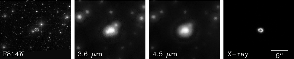
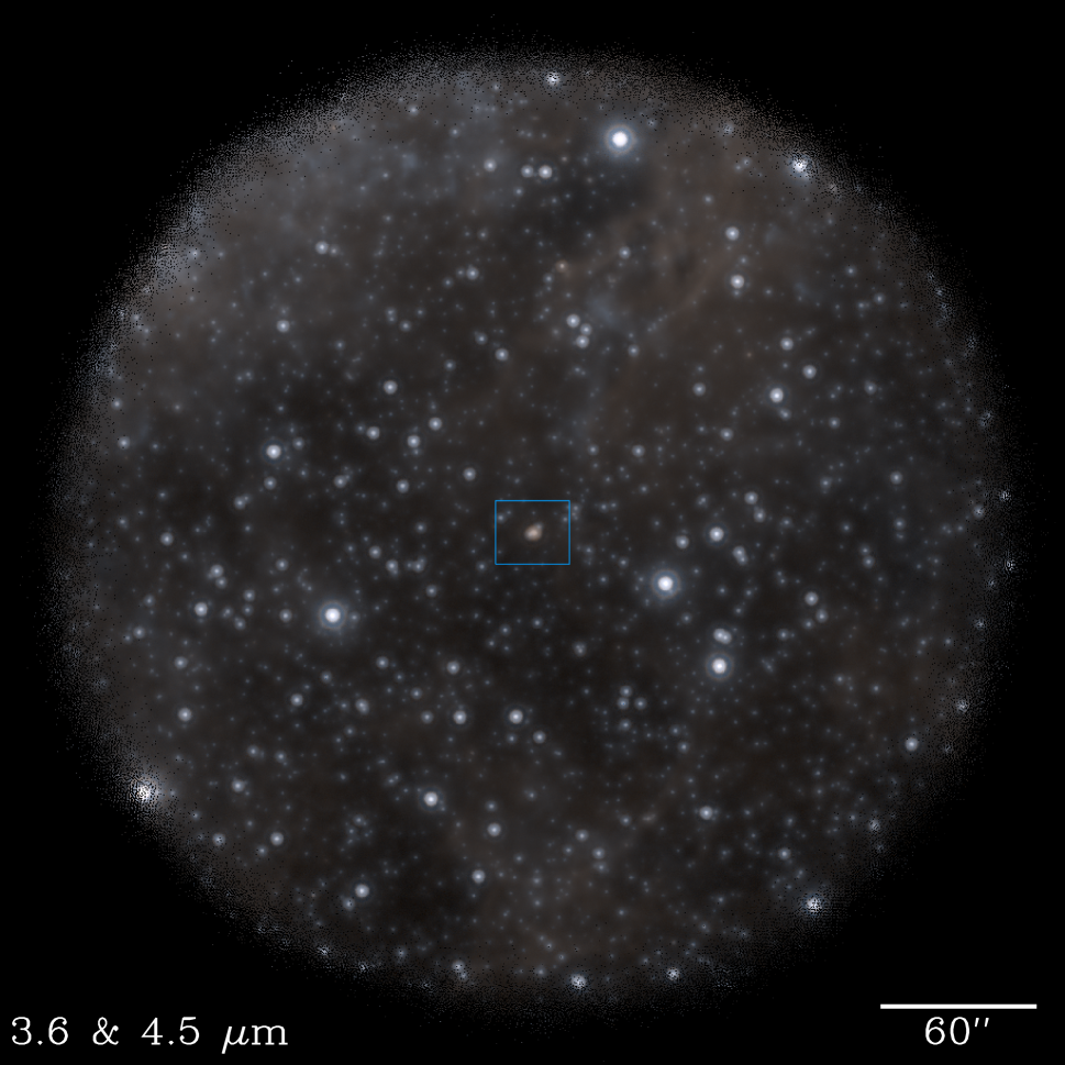
Figure 1.— (top) SN 1987A as seen by Hubble/ACS (F814W, left), Spitzer/IRAC (3.6 and 4.5 $\mu$m, middle), and Chandra/HRC (right). In the IRAC images the angular resolution is $\gtrsim 12$ times worse than the ACS image. Stars 2 and 3 to the NW and SE are only barley resolved from the SN. The ER is elongated, but not resolved. (bottom) The full IRAC 3.6 and 4.5 $\mu$m 2-color image, with SN 1987A centered in the blue box, reveals that the ER is redder than most stars in the field and that it does not show the symmetric PSF that stellar sources exhibit. The optical and IR images are logarithmically scaled; the X-ray image is scaled linearly.

3. Evolution of the IR Continuum

In sections 3.1 and 3.2 we consider the IR evolution in comparison to the X-ray emission. The IR and X-ray emission should be directly related for collisionally heated dust. In Section 3.3 we look at the IR evolution in terms of the dust mass and temperature, without regard for the heating mechanism. Section 3.4 examines the relation between the IR and the optical emission, as potentially related if radiative heating of the dust is important. The “models” in this section are empirical parametric descriptions of the evolution of the IR emission. They can be used as simplified descriptions of the data (e.g. for extrapolation or interpolation) and to identify the behavior of correlations between the IR, and X-ray and optical emission. In some cases the model parameters are related to one or more of the underlying physical parameters of the system.

3.1. Infrared and X-ray Brightness Evolution

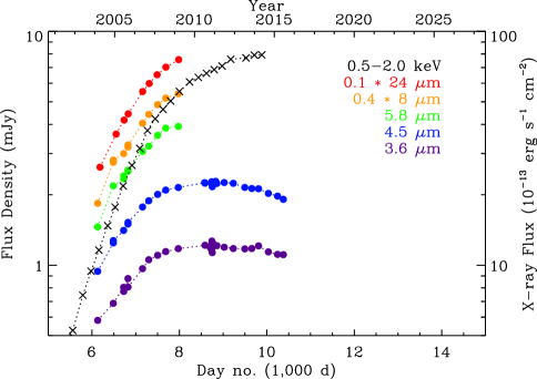
Figure 2.— Evolution of SN 1987A as seen in the 3.6 – 24 $\mu$m flux densities observed with Spitzer, and the soft X-ray fluxes detected with Chandra (Helder et al., 2013). Until 2009, the IR emission had been nearly proportional to the soft X-ray emission. Spitzer/IRAC warm mission data since 2009, have shown that the 3.6 and 4.5 $\mu$m flux densities have deviated from the X-ray trend, and have begun to decline slowly.

Examination of the cryogenic data had indicated that the ratio of 24 $\mu$m IR to X-ray brightness (IRX) was approximately constant between days 6,000 and 8,000. However, continued observations at 3.6 and 4.5 $\mu$m have shown a trend that clearly diverges from the X-ray emission. Figure 2 depicts the observed light curves, as listed in Table 1.

The soft 0.5-2 keV in-band X-ray flux is used throughout for comparison with the IR emission because it is more representative than the harder X-ray emission of the forward shock that propagates through the ER (Dwek et al., 1987). The X-ray data used here are those measured with the Chandra ACIS and published by Helder et al. (2013), to which we add 3 additional epochs of similarly observed and reduced Chandra observations. A more physically motivated comparison might use the integrated X-ray emission of the softer component of 2-component fits to the total X-ray spectrum. The temperature of the soft component varies from 0.2-0.4 keV, and is sufficiently low that the fraction of emission at energies $>2$ keV is negligible. The soft component accounts for $\sim 33\%$ of the flux in the 0.5-2 keV band at day 5,000, rising to $\sim 41\%$ at day 10,000. However, given uncertainties in the corrections of systematic effects in the X-ray data, and the relatively low signal-to-noise of the data at some epochs, both of which affect the spectral fitting, the light curve of the integrated soft X-ray component is much noisier than that of the simple 0.5-2 keV in-band flux.

A strong correlation between the evolution of the X-ray and IR luminosity would be an indication that the mid-IR emission of SN 1987A is from collisionally heated dust in the ER, as both the IR and X-ray emission should be proportional to the mass of shocked material. Figure 3 shows the evolution of flux density, $S(\lambda)$, at each IR wavelength, $\lambda$, compared to scaled versions of the soft X-ray emission, $S(X)$:

$$S(\lambda,t)=a(\lambda)S(X,t).$$ (1)

The empirical fitting parameter $a$ corresponds to a constant IRX ratio (Dwek et al., 1987; Dwek & Arendt, 1992):

$$IRX=n_{dust}\Lambda_{dust}(T_{gas})/n_{H}\Lambda_{gas}(T_{gas}),$$ (2)

where $T_{gas}$ is the gas temperature, $\Lambda_{dust}(T_{gas})$ and $\Lambda_{gas}(T_{gas})$ are the in-band cooling functions of the dust and gas, $n_{dust}$ is the number density of dust grains, and $n_{H}$ is the number density of hydrogen. This is for collisional heating of the dust. For radiative heating, the dust cooling function will depend on the radiation field rather than the gas temperature. The relative importance of radiative vs. collisional heating of dust in supernova remnants has been discussed by Arendt et al. (1999) and Andersen et al. (2011), and in more general circumstances by Bocchio et al. (2013). In all cases we only use data from days 6,000 to 8,000 to determine the parameter $a$. The fit is generally not very good, indicating that the simplest model, given by Equation (1), fails. However, the fit is significantly improved if the model allows a constant flux density offset, $b$:

$$S(\lambda,t)=a(\lambda)S(X,t)+b(\lambda)$$ (3)

as shown in Figure 3. A non-zero value for the parameter $b$ could indicate a systematic error in the measurement of the flux densities of SN 1987A, e.g. error in the subtraction of the contribution of nearby Stars 2 and 3. The parameter $b$ would also account for a component of the SN’s IR or X-ray emission that doesn’t exhibit the same correlated temporal variation as the bulk of the emission.

Using the 24 $\mu$m emission as the reference instead of the X-ray emission provides a check on whether the IR emission is evolving in a consistent manner across all wavelengths. This comparison is also shown in Figure 3. As with the X-ray emission, the shorter wavelengths are consistent with the 24 $\mu$m emission only if a constant emission component is present at each IR wavelength. The fit parameters ($a$, $b$) required here are consistent with those derived from the X-ray comparison given by Equation (3).

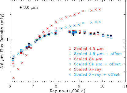
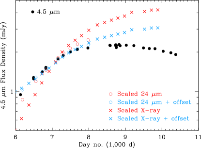
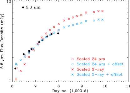
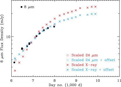
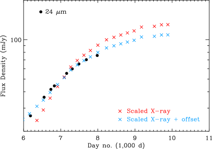
Figure 3.— The evolution of the flux density at 3.6 – 8 $\mu$m (solid black circles) is compared to that at 24 $\mu$m (open circles) and in the soft X-rays ($\times$). In the bottom panel, the 24 $\mu$m evolution (solid black circles) is similarly compared to the soft X-ray evolution. The scaling of the reference emission is determined both directly: $S(\lambda,t)=a(\lambda)\ S(X,t)$ (red symbols), and with the presence of a constant offset: $S(\lambda,t)=a(\lambda)\ S(X,t)+b(\lambda)$ (blue symbols). In all cases, only the data from the cryogenic mission (earlier than day 8,000) are used to determine the scale parameters. Prior to day 8,000, the IR emission can follow the X-ray emission closely if an additional constant term is present. However, at short wavelengths (3.6 and 4.5 $\mu$m) the IR emission deviates after day 8,000.

At 3.6 and 4.5 $\mu$m, the comparison to X-ray emission can be extended over for the longer time intervals from day 6,000 to day 11,000. In these cases, the required constant term is increased such that it accounts for nearly all of the emission at day 6,000, and the ratio of the evolving IR to X-ray emission drops correspondingly. Consistent results are obtained when the 3.6 $\mu$m flux density evolution is compared directly to that at 4.5 $\mu$m.

3.2. IRX Evolution

The empirical models described in the preceding subsection assume that the ratio of IR to X-ray emission should remain constant as the brightness evolves. However, a changing value of IRX could eliminate the need for a strong non-evolving IR emission component in the comparison of IR and X-ray emission. The IRX would be expected to change if the physical conditions (temperature, density, or dust-to-gas mass ratio) in the shocked gas change over time. The ratio of hard to soft X-ray emission has remained nearly constant since day $\sim 6,000$ (see Table 1 of Helder et al., 2013), therefore a decreasing IRX may indicate ongoing grain destruction and evolution of the dust to gas mass ratio $n_{dust}/n_{gas}$. Apart from the explicit dependence of the IRX on the dust to gas mass ratio and the gas temperature, see Equation (2), its numerical value will also depend on the dust grain size distribution, and on the abundances and ionization state of the gas.

A simple model that would allow divergent but related evolution of the IR and X-ray emission can be written as:

$$S(\lambda,t)=\alpha\ S(X,t)(t-t_{0})^{\beta}$$ (4)

where $t_{0}$ represents the time at which the forward shock began interaction with the ER, $\alpha$ is the nominal IRX at that time, and $\beta$ characterizes the evolution of IRX over time. If $\beta=0$ we recover the constant IRX assumption of the model in Equation (1). Assuming $t_{0}$, we can solve for the free parameters $\alpha$ and $\beta$ by performing a linear fit to:

$$\log{[S(\lambda,t)/S(X,t)]}=\beta\log{(t-t_{0})}+\alpha.$$ (5)

For the choice of $t_{0}=4,600$, we derive $\beta=-1.0$ for both 3.6 and 4.5 $\mu$m data. However, at this same $t_{0}$, $\beta$ increases with wavelength, reaching $-0.6$ for the 24 $\mu$m data. Because there is a strong correlation between $t_{0}$ and $\beta$ in this model, we can force $\beta=-1.0$ for each wavelength by making $t_{0}(\lambda)$ a function of wavelength, e.g. $t_{0}(24\ \micron)=3,270$.

The value of $\beta=-1$ is of particular interest. If the volume of the X-ray emitting gas is accumulating as a power law function of $t-t_{0}$, integrated from $t_{0}$ to $t_{1}$, but the volume of the IR emitting region is restricted to a layer representing a finite duration behind the shock front, i.e an integral from $t_{1}-\Delta t$ to $t_{1}$, then the IRX should evolve as $(t-t_{0})^{-1}$ for $\Delta t\ll(t-t_{0})$ (see Fig. 7 of Dwek et al., 2010). The limited thickness of the IR-emitting region would arise if the dust destruction time scale is short compared to the cooling time of the gas.

Figure 4.— Correlation between $t$ and $S(X,t)/S(\lambda,t)$. The $x$-axis intercepts of these linear fits correspond to $t_{0}$ in Equation (6). Averaged over all 5 wavelengths, $\langle t_{0}\rangle=4,376\pm 78$ d.

Therefore if we make the assumption that $\beta=-1$, then we can derive $t_{0}$ and $\alpha$ via a linear fit to:

$$S(X,t)/S(\lambda,t)=\alpha^{-1}(t-t_{0}).$$ (6)

Such fits are shown in Figure 4. If we use this prescription to transform the observed X-ray fluxes to IR flux densities, then the agreement is very good throughout the span of the IR observations (Figure 5). Extrapolation back to earlier times will fail if $t-t_{0}$ is less than the dust destruction timescale. The extrapolation of the 24 $\mu$m emission to later times may be verified in the future with SOFIA (Young et al., 2012) or JWST (Gardner et al., 2006).

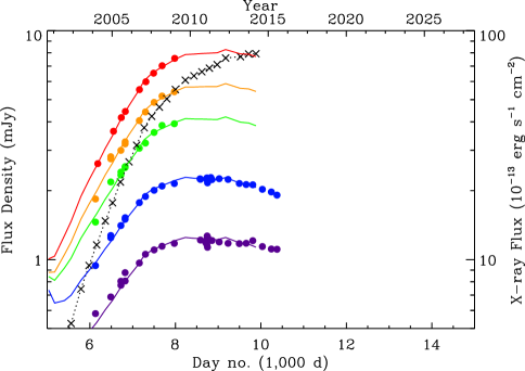
Figure 5.— Observed IR flux densities ($\bullet$) can be well fit by models of the IR emission in the form of $S(\lambda,t)=\alpha S(X,t)/[t-t_{0}(\lambda)]$ (colored lines, coded as in Figure 2). The observed X-ray emission is indicated by the black $\times$ symbols.

3.3. Dust Mass and Temperature Evolution

Comparison of the IR and X-ray emission in the previous subsections indicates that the IRX does not remain constant. The changes may indicate that the decay timescale of the IR emission is much shorter than for the X-ray emission. Decreasing IR emission can occur if the dust cools or is destroyed.

The following models specifically examine whether the IRAC and MIPS data indicate evolution of dust mass, dust temperature, or both. These models use two dust compositions with independent temperatures to fit the IRAC and MIPS SED of SN 1987A at 9 epochs between days 6,000 and 8,000, when observations at all wavelengths were obtained. Guided by the spectral models presented by Dwek et al. (2010), the warm dust component giving rise to the 8-35 $\mu$m emission is assumed to be silicate, with a temperature of $\sim 180$ K, and the hot dust component giving rise to the 3 – 8 $\mu$m emission is assumed to be amorphous carbon, with a temperature of $\sim 460$ K. The hot dust component could alternately be any other composition with a generally featureless spectrum (e.g. iron), and with temperatures that could be as much as $\sim 100$ K lower (Dwek et al., 2010). These components are derived from fits to the Spitzer IRS low resolution spectra (5 – 30 $\mu$m) obtained between days 6,000 and 8,000. The warm dust is consistent with collisional heating by the X-ray emitting gas, and with even small dust grains residing at their equilibrium temperatures (Bouchet et al., 2006; Dwek et al., 2008). The hotter dust can also be collisionally heated, if the grain sizes are sufficiently small, dependent on the unknown dust composition (Dwek et al., 2010). Small carbon grains can reach these high temperatures under thermal equilibrium, but other compositions may require stochastic heating to reach sufficiently high temperatures (Dwek et al., 2010). However, if transiently heated grains are producing the hot component, then they should radiate more strongly at lower temperatures, producing more emission at $\lambda>10$ $\mu$m which would dilute the relative strength of the 10 and 20 $\mu$m silicate features.

The fitting is constrained at different epochs by assuming that the temperature and dust mass evolve as functions of time:

$$S(\lambda,t)=\sum_{i=1}^{2}\frac{4\kappa_{i}(\lambda)}{4\pi d^{2}}M_{i}(t)\pi B_{\nu}[T_{i}(t)]$$ (7)

where $\kappa_{i}(\lambda)$ is the mass absorption coefficient of the dust, $d$ is the distance to the SN, $B_{\nu}(T)=2h\nu^{3}/c^{2}\ 1/(e^{h\nu/kT}-1)$ is the Planck function. The mass absorption coefficient for silicate is taken from Draine & Lee (1984), and for amorphous carbon is from Rouleau & Martin (1991). We choose power law functions of time as a simple means of characterizing the evolution of the mass and temperature of separate warm (silicate) and hot (e.g. carbon) components:

$$M_{i}(t)=M_{i,0}\ (t-t_{1})^{\mu_{i}}$$ (8)

and

$$T_{i}(t)=T_{i,0}\ (t-t_{1})^{\theta_{i}}.$$ (9)

Dwek et al. (2010) illustrate how the mass power law index, $\mu$, changes for idealized shocks expanding into 1-, 2-, or 3-dimensional media, under the cases of free or Sedov expansion, and with or without rapid destruction of dust.

If the temporal evolution is measured with respect to the SN explosion ($t_{1}=0$) then $t-t_{1}$ only varies by a factor of 1.33 from day 6,000 to 8,000, which forces a large value of $\mu_{i}\sim 4-5$ to match the observed change in brightness. It is more realistic to choose $t_{1}$ as the start of the interaction between the blast wave and the ER. Assuming that $t_{1}=$ 5,500 (Dwek et al., 2010), we find that $\mu_{1}=0.87$ (silicate) and $\mu_{2}=0.98$ (carbon). The value of $\mu_{i}\lesssim 1$ could indicate free expansion into a 1-dimensional medium without grain destruction or 2-dimensional medium with grain destruction, or Sedov expansion into a 2 dimensional medium (see Figure 7 of Dwek et al., 2010). For both dust components $\theta_{i}\sim 0$, indicating very little evolution of the temperature.

These results are shown in Figure 6, where the fitted dust temperatures are $T_{1,0}=190$ K for the warm silicate component, and $T_{2,0}=525$ K for the hot amorphous carbon component. These dust temperatures are warmer, though not significantly, than those derived by Dwek et al. (2010). Figure 7 compares the changes in the $\lambda\ /\ 24$ $\micron$ colors of the data and the model. These changes are mostly driven by variation of the relative masses of the warm and hot components, not by changes in the dust temperatures. Figure 8 (top) shows the observed and modeled evolution of the flux densities. Over the fitted interval of days 6,000 – 8,000, the model is in fair agreement with the data. However, extrapolating the model to later times at 3.6 and 4.5 $\mu$m shows a clear deviation between the data and the model.

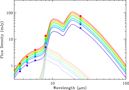
Figure 6.— Fits of a two-temperature, two-composition model to the SED of SN 1987A at 9 different epochs show little apparent evolution of the spectrum. The warm (190 K) component is silicate; the hot (525 K) component is assumed to be amorphous carbon. The evolution of the mass and dust temperature of each component are constrained to be a power law function of $t-t_{1}$, with $t_{1}=5,500$.

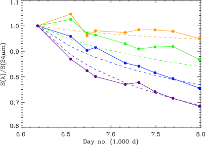
Figure 7.— Evolution of the $\lambda/24\ \micron$ colors for the data ($\bullet$) and the model (dashed lines). The colors are normalized with respect to the color at the first epoch. Results at $\lambda=3.6$, 4.5, 5.8, and 8 $\mu$m are colored violet, blue, green, and orange, respectively. The dashed lines indicate that the model of Equation (7) provides a reasonable representation of the color evolution for days 6,000 - 8,000.

Comparison between the model and observations is shown in Figure 8 (bottom). The ratio between the model and data is constant until about day 7,500, after which the data fall linearly with respect to the model. Thus, we have constructed an altered model for the 3.6 and 4.5 $\mu$m data. Only the hot carbon dust component is used, because the warm silicate dust provides negligible emission at these wavelengths. The dust temperature is still a free parameter, but it is held constant because the previous models suggested very little evolution in temperature. Starting at day 7,500, a linear decrease in the mass is applied. The slope of this decrease indicates a destruction timescale for the dust, $t_{\rm destr}^{-1}$, which is a free parameter to be derived from the data. The form of the model is thus:

$$S(\lambda,t) = \frac{4\kappa(\lambda)}{4\pi d^{2}}M_{0}\ (t-t_{0})^{\mu}\ \pi B_{\nu}(T)$$

$$\hskip 144.54pt{\rm for}\ t<7,500$$

$$= \frac{4\kappa(\lambda)}{4\pi d^{2}}M_{0}\ (t-t_{0})^{\mu}[1-(t-7,500)/t_{\rm destr}]\ \pi B_{\nu}(T)$$

$$\hskip 144.54pt{\rm for}\ t>7,500$$

The fits for this models are shown in Figure 8. The relative accuracy of this model is $\sim 3\%$ at 3.6 $\mu$m and $\sim 2\%$ at 4.5 $\mu$m (shown later in Figure 10).

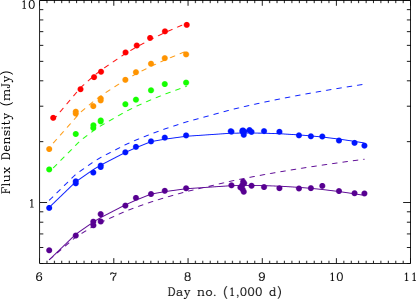
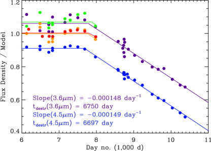
Figure 8.— The top panel shows the evolution of the flux densities for the data ($\bullet$) and the model of Equation (7) (dashed lines). Results at $\lambda=3.6$, 4.5, 5.8, 8, and 24 $\mu$m are colored violet, blue, green, orange, and red, respectively. At later times the extrapolation of the models is not a good fit to the 3.6 and 4.5 $\mu$m data. The bottom panel shows that the ratio between this model and the data is constant at early times, but appears to fall linearly after day $\sim 7,500$. Modifying the model with another factor representing a linear decay after day 7,500 [Equation (3.3)], provides a good fit to the 3.6 and 4.5 $\mu$m data (solid lines) in both the flux densities (top) and the ratios (bottom).

3.4. IR – Optical Evolution

Figure 9 shows the evolution of the IR emission measured by Spitzer compared to the optical emission in the B and R bands measured by HST (Fransson et al., 2015). The correlations are moderately good in both cases, but are better for the B band, which is dominated by the emission lines of H$\gamma$, H$\delta$, and [S II] 0.4069 $\mu$m (Fransson et al., 2015). Figure 10 (upper panels) illustrates that the application of Equation (1), but using the optical instead of the X-ray emission, provides a surprisingly effective model of the IR emission, especially when using the B band optical emission. However, the lower panels of the figure show that the IR emission is more closely matched by the previously discussed functions of the X-ray emission.

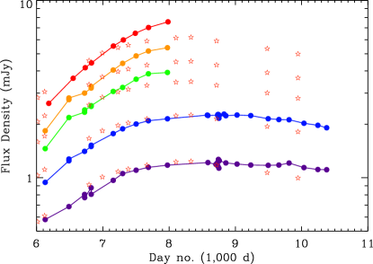
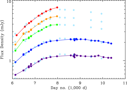
Figure 9.— IR flux density evolution ($\bullet$) in the 3.6, 4.5, 5.8, 8, and 24 $\mu$m bands (violet – red, scaled as in Figure 2) compared to the scaled optical evolution ($\bigstar$) in the R (left) and B (right) bands (Fransson et al., 2015). The evolution of the 3.6 and 4.5 $\micron$ emission is similar to that of the optical emission, especially the B band.

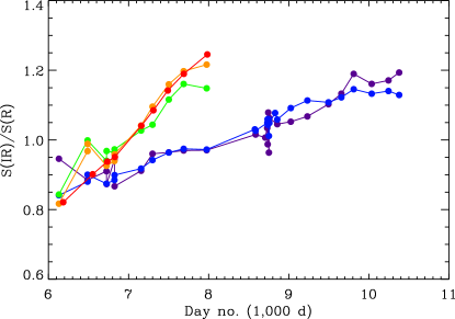
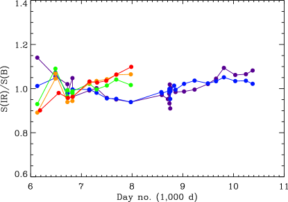
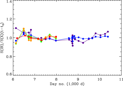
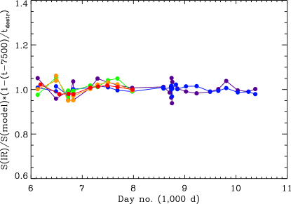
Figure 10.— Ratios of the IR to R and B band emission is shown in the top two panels. The ratios are relatively constant with time, especially at 3.6 and 4.5 $\mu$m and with respect to the B band. The bottom left panel shows that the IR emission is more accurately modeled as proportional to $S(X)/(t-t_{0})$. The bottom right panel shows the ratio between the IR emission of the model of Equation (10) with a roll off after day 7,500. This model provides the most accurate fit to the IR data.

These correlations between the optical and the IR emission may indicate the IR and optical emission originate in the same, or closely related, regions of the shocked ER. However, examination of the radiative luminosity of the SN at various wavelengths indicates that it is unlikely the dust heating can be predominantly radiative. Radiation from the ER is dominated by UV - X-ray emission with a total 0.01 - 8 keV luminosity of $\sim 1,460\ L_{\sun}$ (France et al., 2015). The ER dust has an integrated IR luminosity of $\sim 1,450\ L_{\sun}$. Radiative heating would require that half of the ER emission is absorbed by dust within the ring. The required optical depth is inconsistent with gas phase abundances indicating little depletion into dust (e.g. Mattila et al., 2010) and spectral analysis which requires only Galactic + LMC line of sight extinction corrections (e.g. Pun et al., 2002; Gröningsson et al., 2008b).

4. Evolution of the IR Emission Lines

4.1. Line Identification

The atomic spectral lines seen in the mid-IR are usually the ground state fine-structure transitions of various ionized species. One or more higher-lying H recombination lines are seen, and one excited state transition of [Fe II] is detected. Cutouts of the lines in the SH and LH data are shown in Figure 11, and lines in the SL and LL data are shown in Figure 12. Here we only discuss the lines, as the continuum in the SL and LL spectra has been analyzed by Bouchet et al. (2006) and (Dwek et al., 2008, 2010). The continuum in the SH and LH data adds no new information and is less reliably measured as the concatenation of many spectral orders.

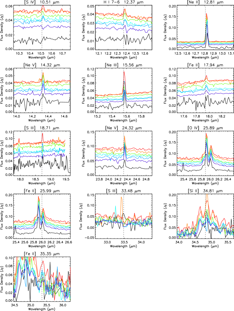
Figure 11.— Spectral lines of SN 1987A as seen in the high spectral resolution SH+LH Spitzer IRS data. The rising continuum levels correlate with the date of the observations. The dotted lines at constant wavelength indicate the rest wavelength of each line. The spectra are not adjusted for the systemic velocity of the ER, $\sim 287$ km s^-1 (Gröningsson et al., 2008a). For each line, the wavelength range displayed corresponds to a velocity range of [-7,500, +7,500] km s^-1.

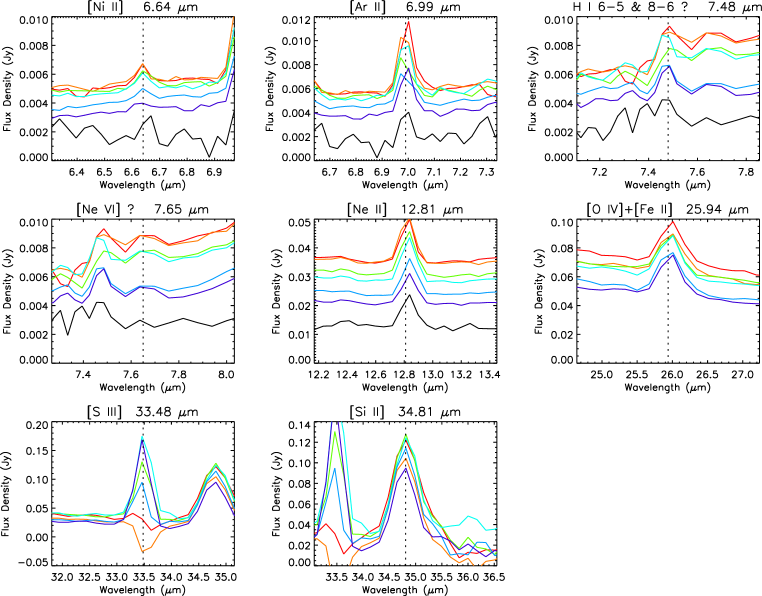
Figure 12.— Spectral lines of SN 1987A as seen in the low spectral resolution SL+LL Spitzer IRS data. The rising continuum levels correlate with the date of the observations. The dotted lines at constant wavelength indicate the rest wavelength of each line. The spectra are not adjusted for the systemic velocity of the ER, $\sim 287$ km s^-1 (Gröningsson et al., 2008a). For each line, the wavelength range displayed corresponds to a velocity range of [-15,000, +15,000] km s^-1.

Nearly all of the observed emission lines can be attributed to the emission ring, as the widths of most lines seem to be unresolved at the $R\sim 600$ resolution of the IRS SH and LH modules. However this spectral resolution is insufficient to distinguish between the ionized but unshocked component of the ring and the shocked component of the ring, which are clearly seen as narrow (FWHM $\sim$ 10 km s^-1) and intermediate (FWHM $\sim$ 300 km s^-1) width components in high resolution optical spectra (e.g. Gröningsson et al., 2008a).

One apparent exception is the [Si II] line at 34.81 $\micron$. At all epochs (barring the low signal to noise data of the initial observations at day 6,109), this emission line seems to be flanked by a pair of lines at velocities of $\pm$ 1,700 km s^-1 with respect to the central component. The background spectra do not show any indication of the shifted lines. The velocities of the flanking lines are large compared to the velocities associated with shocked emission ring, but fairly small compared to the velocity of the SN ejecta. The distinctness of the flanking lines implies that they are not produced by an expanding spherical distribution (either a shell or a filled sphere) of material. Either a bi-polar or an expanding ring-shaped distribution could produce the flanking lines. The homunculus in the $\eta$ Car nebula is an example of a bipolar structure in the circumstellar medium of a massive star. However its expansion velocity is lower, at $\sim 600-800$ km s^-1 (e.g. Gehrz & Ney, 1972; Meaburn et al., 1987). A ring-shaped distribution would also produce a plateau of emission between the flanking lines, but the presence of the central line makes it difficult to determine whether or not a plateau exists. Furthermore, the strength of the central component and any underlying plateau may be affected by imperfect subtraction of the background [Si II] emission which is strong in the vicinity of SN 1987A. None of the other lines show this velocity structure, with the possible exception of the [Fe II] 25.99 $\micron$ line.

The high resolution spectra show a complicated blend of lines at 26 $\micron$. The strongest two components are [O IV] 25.89 $\micron$ and [Fe II] 25.99 $\micron$. Both of these identifications are confirmed by having velocity shifts in agreement with other unblended lines in the spectra. Additionally, there appear to be wings on both the red and blue sides of the [O IV] and [Fe II] pair. The blue wing may be a separate line that is only marginally resolved from the [O IV] line. Bouchet et al. (2006) had pointed out that this feature could be [F IV] 25.83 $\micron$ (based on the line list used by SMART). However, we now believe the [F IV] identification is unlikely because (a) other line lists cite a wavelength of 25.76-25.773 for this line, making the wavelength agreement worse, (b) no other fluorine lines are observed ([F I] 24.75, [F II] 29.33, nor [F V] 13.40 $\micron$) despite the fact that they lie in spectral regions with low noise, and (c) there are many other elements that are normally much more abundant than fluorine that are not seen in the spectrum. If not [F IV], then this blue wing is probably a velocity shifted component of [O IV] or [Fe II]. If [O IV], it is a velocity structure not seen in any other lines. If [Fe II], it may correspond to the flanking lines of [Si II], however there is no corresponding feature on the red side. The red wing that is present on the 26 $\micron$ complex is much broader than the blue wing. We presume that it represents a higher velocity distribution of [Fe II]. The 26 $\micron$ complex was fitted iteratively for [O IV], [Fe II], [F IV] (or blue wing component), and the broad [Fe II] component, subtracting each line before fitting the next.)

The complex of [Si II] and [Fe II] lines at 35 $\micron$ was also fitted iteratively. The central [Si II] line was fitted first. It usually has the largest width, which is possibly influenced by blending with the red and blue shifted components. In contrast, a simultaneous fit for all three [Si II] lines often derives a much smaller width and a proportionally small flux for the central [Si II] line. Thus the individual [Si II] line fluxes may be uncertain by nearly a factor of 2 due to systematic effects, but the integrated flux of all three [Si II] lines is consistent within $5\%$. The gaussian fits to all lines in the SH and LH spectra at all epochs are listed in Table 2.

The IRS SL module provides coverage of the $5<\lambda<10\ \micron$ region which is inaccessible with the SH module. The strongest line seen here is [Ar II] 6.99 $\micron$ which is clearly seen at all dates. The [Ni II] 6.64 $\micron$ line (the single ground state fine structure transition of this species) is not so clear in the earliest data, but seems to be present in the later observations. Additional lines may be present near 7.48 and 7.65 $\micron$. These features lie near the ends of the spectral orders of the IRS modules and are thus somewhat less reliable, but they do seem be present in multiple orders and at many or all epochs. The shorter wavelength feature may be a blend of the H I 6-5 and 8-6 transitions. This identification is supported by the weak detection of the H I 7-6 transition in the SH data. The 7.65 $\micron$ feature could be [Ne VI], which would make it the most highly ionized species that we observe.

4.2. Line Evolution

Figure 13 illustrates the changes in the lines fluxes over a 5-year period for those lines seen in the SH and LH spectra. When present, the intensities of lines in the background are also plotted. This provides an indication of the potential systematic errors in measurements due to the different slit orientations and background fields at each epoch. The comparison with the background also shows that the SN 1987A line measurements are suspect or impossible when the background intensity is $\sim$2 or more times brighter then the SN (e.g. [S IV], [Ne III], [S III], and maybe [Si II]). We have fitted these light curves with three models. The first model is that the line intensity is proportional to the continuum intensity: $F_{line}=A\ F_{24\micron}$, and is shown as a dotted line in each panel of the figure. The second model is that the line intensity is constant: $F_{line}=B$, as indicated by the dashed lines. The third model uses 2 parameters to model the evolution as a linear function of time: $F_{line}=\beta+\alpha\ t$ (dash-triple-dot line in the figure). Table 3 lists the derived parameters of the fits for each line and each model. The probabilities, $P(<\chi^{2})$, are the probability of finding a smaller value of $\chi^{2}$ than the observed $\chi^{2}$ under the assumption that the data are a random sampling of the model. Thus $P(<\chi^{2})\sim 1$ indicates the data are very unlikely to be related to the given model. Figure 14 and Table 4 provide the results for the comparable analysis of the low resolution spectral lines.

The formal results of the fitting procedures indicate that the evolution of the line intensities are usually consistent with a constant value, although in several cases uncertainties are large enough that the intensities are also consistent with the models which increase over time. The only lines to exhibit significantly increasing intensities are the H I 7–6 and the broad [Fe II] lines. The rising intensities correlated with the continuum may be associated from the increasing volume of the shocked portion of the ER. The line intensities that are flat (or possibly declining) may be dominated by emission for unshocked regions of the ER, corresponding to the narrow components seen in the optical emission lines (Gröningsson et al., 2008b).

The evolution of the IR emission lines has also been compared to the evolution of the H$\alpha$ line components from the shocked and unshocked (pre-shock) portions of the ER (Fransson et al., 2015). Figure 15 shows the rising, then cresting, H$\alpha$ intensity of the shocked material of the ER compared to scaled versions of the IR lines that appear to show similar trends. The other IR lines seems to show relatively little evolution and appear to be more consistent with the emission from the unshocked portion of the ER (Figure 16).

4.3. Gas Diagnostics

The ratio of the [Ne V] lines is the only good density diagnostic these data provide since other useful line pairs ([S III], [Ne III], [Ar III], [Ar V]) are either corrupted by the bright background or absent from the SN spectrum at this sensitivity. The ratio of the [Ne V] line intensities at the first epoch is $R_{(14.3/24.3)}=1.5\pm 0.6$, which implies an electron density of $\sim 3\times 10^{3}$ cm^-3 (for $T_{e}\sim 10^{4}$ K) (see Figure 17). However, for all subsequent observations the ratio has a mean value of $R_{(14.3/24.3)}=0.63\pm 0.05$ which lies below the low density limit ($n_{e}<10^{3}$ cm^-3) unless the gas temperature is $T_{e}<1,300$ K.

Similarly low density and temperature are inferred from the ratio of H$\alpha$/H(7-6) $\approx 129$, assuming case B recombination (Hummer & Storey, 1987) (Figure 18). This observed ratio is the scale factor between the H(7-6) 12.37 $\mu$m light curve as measured at high resolution with the IRS, and the H$\alpha$ light curve of the shocked gas measured with HST (Fransson et al., 2015). The possible blend of the H(6-5) and H(8-6) lines observed near 7.48 $\mu$m in the low resolution IRS spectrum suggests slightly higher densities and/or temperatures, but this measurement is less reliable.

Dwek et al. (2008) had concluded that the collisionally heated dust must reside in gas with $T_{e}\approx 3.5\times 10^{6}$ K and $n_{e}\approx(0.3-1)\times 10^{4}$ cm^-3. This is denser, hotter, and at higher pressure than the line emitting regions, suggesting that the observed IR line emission does not arise for the same part of the ER as the dust continuum emission. To reach equilibrium temperatures of $T\approx 180$ K for silicate grains, collisional heating at the low gas temperatures implied by the emission line ratios would require densities of $n_{e}\gtrsim 10^{6}$ cm^-3 (Bouchet et al., 2006; Dwek et al., 2008). Such high densities are ruled out by the observed line ratios (Figures 17 and 18).

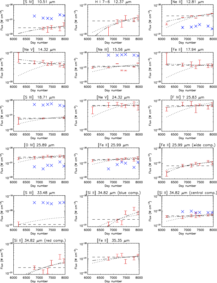
Figure 13.— Evolution of spectral line fluxes of SN 1987A as seen in the SH+LH Spitzer IRS data. Measured fluxes are indicated with 1-$\sigma$ error bars. The $\times$ symbols denote flux measurements of the subtracted background line emission, which in some cases is dominant. The dotted line shows the evolution of the 24 $\micron$ flux density after being normalized to fit the line fluxes. The dashed lines are models of constant line intensity, and the dash-triple-dotted lines indicate models where intensity is linear with time.

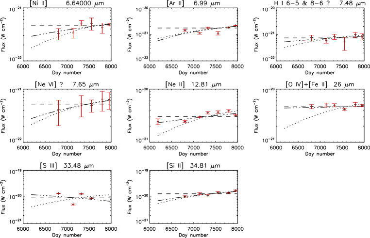
Figure 14.— Evolution of spectral line fluxes of SN 1987A as seen in the SL+LL Spitzer IRS data. Error bars show 1-$\sigma$ uncertainties. The dotted line shows the evolution of the 24 $\micron$ flux density after being normalized to fit the line fluxes. The dashed lines are models of constant line intensity, and the dash-triple-dotted lines indicate models where intensity is linear with time.

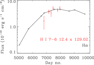
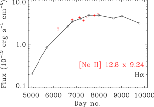
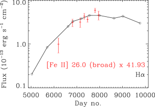
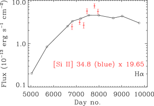
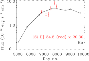
Figure 15.— IR emission lines with markedly increasing fluxes (+ symbols with error bars) are reasonably correlated with the evolution of the H$\alpha$ flux (circles) from the shocked ER material (Fransson et al., 2015). The scale factors applied to the IR lines fluxes are given in the legend for each panel.

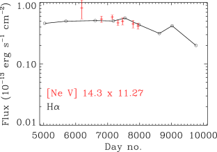
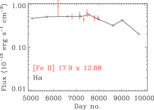
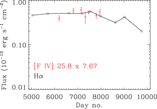
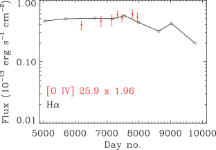
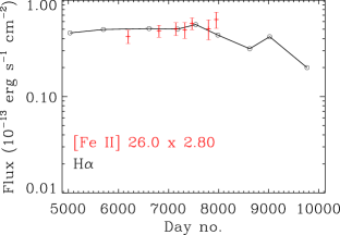
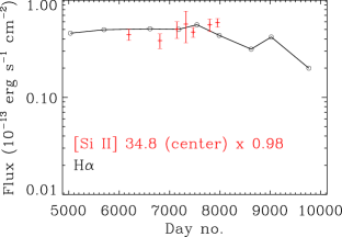
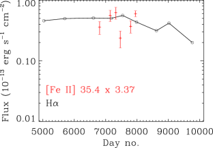
Figure 16.— IR emission lines with approximately constant fluxes (+ symbols with error bars) are reasonably correlated with the evolution of the H$\alpha$ flux (circles) from the unshocked ER material (Fransson et al., 2015). The scale factors applied to the IR lines fluxes are given in the legend for each panel.

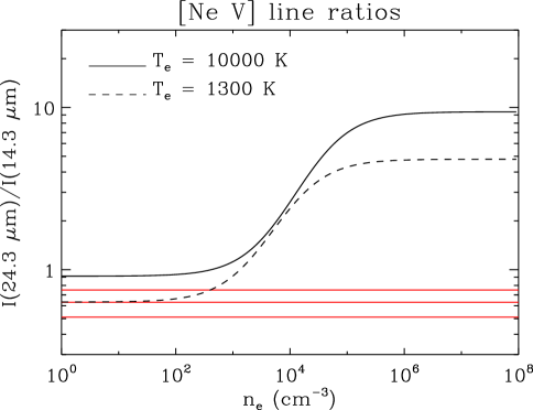
Figure 17.— Expected [Ne V] line ratios as a function of density for $T_{e}=10^{4}$ and 1,300 K. The observed line ratios are $\sim 1.5\pm 0.6$ at day 6,190 and $\sim 0.63\pm 0.12$ at later times (red lines).

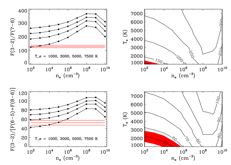
Figure 18.— SN 1987A H recombination line ratios compared to Case B recombination (Hummer & Storey, 1987). (upper left) the Case B ratio of H$\alpha$/H(7-6) is plotted as a function of density for various temperatures (1,000 K $<T_{e}<$ 7,500 K). The observed line ratio and its $\pm 1\sigma$ uncertainty range are shown by the red lines. (upper right) The same H$\alpha$/H(7-6) is plotted as contours as a function of $n_{e}$ and $T_{e}$. The $\pm 1\sigma$ uncertainty range is indicated by the shaded red band at the low temperature and density limits of the calculations. (lower panels) These show similar plots for the case B and observed line ratios of H$\alpha$ / [H(6-5)+H(8-6)].

5. Discussion

5.1. Continuum (Dust) Evolution

With the long interval of observations now available, it has become clear that the SN emission at 3.6 and 4.5 $\mu$m has peaked and is now in decline. This suggests, that, as for the optical emission (Fransson et al., 2015), the SN blast wave has sent shocks through the bulk of the material in the ER, and the emission of any remaining swept up material is insufficient to make up for the fading of the ER material that has already been shocked. Despite the likelihood that the emitting dust is collisionally heated in the hot gas, it is also clear that 3.6 and 4.5 $\mu$m emission is not tracking the X-ray emission. If the X-ray emission is reaching a peak, it is $>1,000$ days after the IR peak. The simplest explanation for this evolving IRX ratio is that the dust is being destroyed on timescales of a few years, $\tau_{\rm sput}\approx 10^{6}a(\micron)/n_{\rm H}({\rm cm}^{-3})$ yr (Draine & Salpeter, 1979) which is shorter than the cooling time for the X-ray emitting gas: $\sim 5-30$ yr (Dwek et al., 2010). The apparently short sputtering timescale and high dust temperature for the grains the produce the 3.6 and 4.5 $\mu$m emission are most easily achieved by relatively small grains compared to those that produce the 24 $\mu$m emission. However, the exact sizes depend on the unknown composition of the dust and on more precise estimates of the sputtering timescale (see Dwek et al., 2010). Bocchio et al. (2012) show that very small amorphous hydrocarbons and PAHs have even shorter lifetimes in a hot gas than classical sputtering calculations predict. Although the spectra of SN 1987A show no indications of the PAH emission features, the physical mechanisms they consider may also act to decrease the lifetimes of small grains of other compositions.

The 5 – 30 $\mu$m spectrum had been used to estimate the mass of warm dust in the ER as $1.2\times 10^{-6}~{}M_{\sun}$ at day 7,554 (Dwek et al., 2010). Because there was little change in the dust temperature, this mass scales linearly with the evolving IR flux density. The spectral fits in Dwek et al. (2010, Figures 4 and 5) suggest that the dust responsible for the 3.6 and 4.5 $\mu$m emission is $\sim 2$ times warmer and $\sim 100$ times fainter (in the Rayleigh-Jeans tail). Therefore the mass of this hot dust is only $\sim 0.5\%$ of the total dust in the ER, with a large uncertainty depending on the actual emissivity of these grains of uncertain composition. (If the hot dust component is stochastically heated rather than at equilibrium temperatures, then its total dust mass would be larger because only a small fraction of the dust would be contributing to the short wavelength emission.) The evident destruction of this hot dust component is not necessarily indicative of significant reduction in the total dust mass of the ER.

The IRX evolution model of Equation (6), as shown in Figure 4, indicates a correlation between wavelength and $t_{0}$. The parameter $t_{0}$ is the extrapolated time at which the IR emission began the trend of $S(IR,t^{\prime})\sim S(X,t^{\prime})/t^{\prime}$ where $t^{\prime}=t-t_{0}$. It is unclear if this trend really does extrapolate back to $t_{0}$, but if so, we can suggest two potential reasons for the correlation of wavelength and $t_{0}$.

The first possibility is that the UV flash from the SN has preferentially evaporated small dust grains, creating a gradient in the size distribution of dust grains as a function of radius as described by Fischera et al. (2002). In this case, the initial (near day 3,200) IR emission from the interaction of the blast wave with the ER should be dominated by relatively large grains. These grains do not get heated to very high temperatures, and may thus produce strong 24 $\mu$m emission but little emission at $<10$ $\mu$m. As the blast wave expands further into the ring, near day 4,500 it may begin encountering smaller grains that were sufficiently distant or shielded from the SN to have escaped evaporation. These smaller grains would be heated to higher temperatures capable of producing the observed emission and IRX trends at 3.6 and 4.5 $\mu$m. If this scenario is valid it would suggest that the small grains emitting at the shortest wavelengths are not carbonaceous. Fischera et al. (2002) show that the UV flash is significantly less effective at evaporating graphite grains than silicate or iron grains. Therefore, small carbonaceous grains would be encountered at earlier times than large (or any) silicate grains.

The second possibility is that grain-grain collisions in the post-shock gas are fragmenting larger grains into smaller ones. The result $t_{0}=$ 3,251 at 24 $\mu$m would be interpreted as there having been sufficient time for all of the largest grains to be destroyed in the post-shock region. The result $t_{0}=$ 4,523 at 3.6 $\mu$m would indicate that smaller grains are present for an additional $\sim$3.5 yr after the destruction of the largest grains. However, grain-grain collisions are generally most effective in the cases of much slower shocks (e.g. 10s of km s^-1) propagating into media at least as dense as the ER. In these higher velocity shocks, thermal and non-thermal sputtering would be the dominant destruction mechanism (Dwek et al., 2010), and small grains should be destroyed more rapidly than the larger grains.

5.2. Emission Line (Gas) Evolution

The observed IR emission lines are mostly collisionally excited fine structure transitions in the ground state of various ions. The lines identified are typical of those seen in other supernova remnants (Oliva et al., 1999; Arendt et al., 1999; Temim et al., 2006; Neufeld et al., 2007; Smith et al., 2009; Andersen et al., 2011; Ghavamian et al., 2012; Sankrit et al., 2014). The accuracy of the measurement of the lines strengths is limited by the modest signal-to-noise ratio of some lines, and the presence of strong (sometimes dominant) and structured background emission from the ISM in some of the lines.

The evolution of the IR emission lines is puzzling. Many of the emission lines seem to show little evolution, consistent with the minimal evolution of optical emission lines from the unshocked portion of the ER (Figure 16). However, these lines include highly ionized species such as Ne V and O IV, which have much higher ionization potentials than other lines attributed to the unshocked portion of the ER.

Another puzzle is presented by the higher velocity components of the Fe II and Si II lines. These lines may originate in gas phase material, but they may also represent material that has been eroded from dust grains. The high velocities suggest shocked material, and indeed these lines do correlate with the rising intensity of the shocked H$\alpha$ emission, as well as the increasing 24 $\mu$m (dust) flux density. The velocity structures of these two lines is somewhat mysterious. It is not clear why the Si II should show distinct high and low velocity components, whereas the Fe II line seems to show a simple broad component which would be expected for a spherical distribution of material. The lines may indicate the presence an expanding fossil remnant from the SN precursor as in $\eta$ Carinae. The Fe lines may be from a more symmetrical fossil remnant than the Si lines. $\eta$ Car has undergone multiple eruptions (at least 3 in the last $\sim 200$ years), not all producing the same geometry (see Smith & Gehrz, 1998, 2000). Alternatively, it may be that these lines originate in the SN ejecta, rather than the ER or other circumstellar structures, in which case, the velocity structures of the Si II lines may reflect uneven distribution of Si in the ejecta. The presence of the redshifted component would indicate that the ejecta are not (uniformly) optically thick at $\sim 35$ $\mu$m.

The final puzzle presented by the emission lines is that both the H recombination lines and the Ne V lines suggest low densities ($n_{e}\lesssim 10^{3}$ cm^-3) and low temperatures ($T_{e}\lesssim 2,500$ K). The densities are much lower than estimated for the ER from pre-interaction observations (e.g. Plait et al., 1995) or analysis of the earliest hot spot (Michael et al., 2000; Pun et al., 2002). However, Gröningsson et al. (2008b) find indications of densities nearly this low for the narrow line emission of the unshocked material, and Mattila et al. (2010) invoke a $10^{2}$ cm^-3 component distributed over a wider area to account for the evolution of high-ionization lines at late times (days 5,000 – 7,500). So the densities suggest that the H and Ne emission lines may arise from the regional outside of the ER, perhaps associated with multiple ejections from the precursor. However implied the low gas temperature remains at odds with prior analyses, and seems unlikely since the recombination rate for Ne V is several times higher than the cooling rate (assuming solar abundances; Osterbrock, 1989; Draine, 2011).

6. Summary

More than ten years of Spitzer broadband mid-IR photometry of SN 1987A have now shown that the 3.6 and 4.5 $\mu$m emission associated with the ER has peaked and is now in a declining phase.

The IR emission is not directly proportional to the X-ray emission, which would be expected if the dust is collisionally heated and the dust-to-gas mass ratio remains constant.

The IRX does seem to evolve as $(t-t_{0})^{-1}$, which is consistent with an accumulating mass of shocked gas behind the ER shocks, but a finite zone of IR emission, limited by the dust destruction timescales that are short compared to the gas cooling timescale.

The dust mass itself can grow linearly as $(t-t_{0})$ at early times (the dust temperature remains constant), but must begin decreasing after about day 7,500 to match the 3.6 and 4.5 $\mu$m light curves.

The time $t_{0}$ and its apparent variation with wavelength can be interpreted either as a) an indication of evaporation of small grains by the UV flash, or b) the initial preferential destruction of large grains via grain-grain collisions in the post-shock gas.

The IR light curve is also in fair agreement with the latest optical light curves (particularly the B band), which have indicated that the peak of the interaction with the ER has passed.

IR emission lines seem to arise from two regions. One set of lines is characterized by relatively constant emission, as matched by the evolution of narrow (pre-shock) optical emission lines. The other set of lines includes odd high-velocity components, and seems to match the evolution of the optical lines from the post-shock ER regions. These lines may indicate possible fossil circumstellar remnants, distinct from the ER, produced by the SN precursor.

Table 1SN 1987A Flux Densities

Day	IRAC				MIPS
Number	$S(3.6\ \micron)$	$S(4.5\ \micron)$	$S(5.8\ \micron)$	$S(8\ \micron)$	$S(24\ \micron)$
6130.09	0.99 $\pm$ 0.01	1.20 $\pm$ 0.01	1.62 $\pm$ 0.02	4.69 $\pm$ 0.03	$\cdots$
6184.08	$\cdots$	$\cdots$	$\cdots$	$\cdots$	26.3 $\pm$ 1.8
6487.93	1.10 $\pm$ 0.01	1.51 $\pm$ 0.01	2.34 $\pm$ 0.04	6.98 $\pm$ 0.04	$\cdots$
6487.94	$\cdots$	1.53 $\pm$ 0.02	$\cdots$	7.13 $\pm$ 0.07	$\cdots$
6551.91	$\cdots$	$\cdots$	$\cdots$	$\cdots$	36.4 $\pm$ 1.9
6724.25	1.21 $\pm$ 0.01	1.67 $\pm$ 0.01	2.50 $\pm$ 0.04	7.59 $\pm$ 0.05	$\cdots$
6725.68	1.18 $\pm$ 0.02	$\cdots$	2.57 $\pm$ 0.05	$\cdots$	$\cdots$
6734.33	$\cdots$	$\cdots$	$\cdots$	$\cdots$	41.7 $\pm$ 1.9
6823.54	1.29 $\pm$ 0.01	1.76 $\pm$ 0.01	2.68 $\pm$ 0.04	8.10 $\pm$ 0.06	$\cdots$
6824.65	1.22 $\pm$ 0.01	1.78 $\pm$ 0.01	2.71 $\pm$ 0.04	8.26 $\pm$ 0.05	$\cdots$
6828.53	$\cdots$	$\cdots$	$\cdots$	$\cdots$	44.4 $\pm$ 1.9
7156.35	1.38 $\pm$ 0.01	2.03 $\pm$ 0.01	3.23 $\pm$ 0.02	10.21 $\pm$ 0.04	$\cdots$
7158.88	$\cdots$	$\cdots$	$\cdots$	$\cdots$	55.3 $\pm$ 1.8
7298.80	1.47 $\pm$ 0.01	2.15 $\pm$ 0.01	3.39 $\pm$ 0.02	11.13 $\pm$ 0.04	$\cdots$
7309.70	$\cdots$	$\cdots$	$\cdots$	$\cdots$	59.8 $\pm$ 1.9
7489.68	$\cdots$	$\cdots$	$\cdots$	$\cdots$	65.2 $\pm$ 1.9
7502.04	1.51 $\pm$ 0.01	2.27 $\pm$ 0.01	3.75 $\pm$ 0.02	12.24 $\pm$ 0.05	$\cdots$
7687.35	1.55 $\pm$ 0.01	2.36 $\pm$ 0.01	4.02 $\pm$ 0.02	13.04 $\pm$ 0.04	$\cdots$
7689.55	$\cdots$	$\cdots$	$\cdots$	$\cdots$	70.3 $\pm$ 1.9
7974.80	1.59 $\pm$ 0.01	2.41 $\pm$ 0.01	4.08 $\pm$ 0.02	13.61 $\pm$ 0.03	$\cdots$
7983.16	$\cdots$	$\cdots$	$\cdots$	$\cdots$	75.7 $\pm$ 1.9
8576.21	$\cdots$	2.51 $\pm$ 0.02	$\cdots$	$\cdots$	$\cdots$
8585.63	1.63 $\pm$ 0.01	2.50 $\pm$ 0.01	$\cdots$	$\cdots$	$\cdots$
8706.09	1.60 $\pm$ 0.02	$\cdots$	$\cdots$	$\cdots$	$\cdots$
8730.61	1.63 $\pm$ 0.02	$\cdots$	$\cdots$	$\cdots$	$\cdots$
8732.20	$\cdots$	2.51 $\pm$ 0.02	$\cdots$	$\cdots$	$\cdots$
8735.25	$\cdots$	2.53 $\pm$ 0.02	$\cdots$	$\cdots$	$\cdots$
8736.63	1.57 $\pm$ 0.02	$\cdots$	$\cdots$	$\cdots$	$\cdots$
8738.06	$\cdots$	2.50 $\pm$ 0.01	$\cdots$	$\cdots$	$\cdots$
8743.47	1.68 $\pm$ 0.02	2.53 $\pm$ 0.02	$\cdots$	$\cdots$	$\cdots$
8751.53	1.54 $\pm$ 0.02	2.42 $\pm$ 0.02	$\cdots$	$\cdots$	$\cdots$
8757.27	1.66 $\pm$ 0.02	2.50 $\pm$ 0.01	$\cdots$	$\cdots$	$\cdots$
8829.32	$\cdots$	2.54 $\pm$ 0.02	$\cdots$	$\cdots$	$\cdots$
8856.29	1.62 $\pm$ 0.01	2.50 $\pm$ 0.01	$\cdots$	$\cdots$	$\cdots$
9024.97	1.60 $\pm$ 0.01	2.52 $\pm$ 0.01	$\cdots$	$\cdots$	$\cdots$
9232.27	1.59 $\pm$ 0.01	2.50 $\pm$ 0.01	$\cdots$	$\cdots$	$\cdots$
9495.25	1.58 $\pm$ 0.01	2.41 $\pm$ 0.01	$\cdots$	$\cdots$	$\cdots$
9656.20	1.59 $\pm$ 0.01	2.39 $\pm$ 0.01	$\cdots$	$\cdots$	$\cdots$
9810.19	1.62 $\pm$ 0.01	2.38 $\pm$ 0.01	$\cdots$	$\cdots$	$\cdots$
10034.95	1.55 $\pm$ 0.01	2.29 $\pm$ 0.01	$\cdots$	$\cdots$	$\cdots$
10244.63	1.52 $\pm$ 0.01	2.23 $\pm$ 0.01	$\cdots$	$\cdots$	$\cdots$
10377.66	1.52 $\pm$ 0.01	2.17 $\pm$ 0.01	$\cdots$	$\cdots$	$\cdots$

Note. — units = Jy

Table 2High Resolution Lines

Day number	Species	$\lambda_{0}$ ($\micron$)	$\lambda$ ($\micron$)	$v$ (km s-1)	FWHM ($\micron$)	Flux (10-22 W m-2)
6190	[Ne II]	12.81355	$12.8305\pm 0.0004$	397.	$0.0189\pm 0.0004$	$24.0\pm 1.6$
6190	[Ne V]	14.32170	$14.3369\pm 0.0049$	318.	$0.0465\pm 0.0050$	$7.3\pm 2.4$
6190	[Ne III]	15.55510	$15.5765\pm 0.0009$	413.	$0.0176\pm 0.0007$	$10.5\pm 1.3$
6190	[Fe II]	17.93595	$17.9695\pm 0.0046$	561.	$0.0365\pm 0.0048$	$6.8\pm 2.7$
6190	[S III]	18.71300	$18.7411\pm 0.0034$	451.	$0.0251\pm 0.0041$	$5.3\pm 2.6$
6190	[Ne V]	24.31750	$24.3404\pm 0.0022$	283.	$0.0304\pm 0.0026$	$4.8\pm 1.2$
6190	[F IV]?	25.83000	$25.8354\pm 0.0021$	63.	$0.0456\pm 0.0021$	$5.1\pm 0.7$
6190	[O IV]	25.89030	$25.9069\pm 0.0026$	192.	$0.0538\pm 0.0027$	$20.2\pm 3.1$
6190	[Fe II]	25.98829	$26.0065\pm 0.0031$	210.	$0.0616\pm 0.0031$	$15.0\pm 2.4$
6190	[Fe II] (broad)	25.98829	$26.0831\pm 0.0051$	1094.	$0.0406\pm 0.0050$	$2.4\pm 0.9$
6190	[S III]	33.48100	$33.4806\pm 0.0189$	-4.	$0.1131\pm 0.0201$	$13.9\pm 6.8$
6190	[Si II]	34.81520	$34.8546\pm 0.0030$	339.	$0.0713\pm 0.0029$	$45.5\pm 5.8$
6809	[S IV]	10.51050	$10.5222\pm 0.0020$	334.	$0.0147\pm 0.0018$	$-1.6\pm 0.6$
6809	H I 7-6	12.37190	$12.3822\pm 0.0011$	250.	$0.0095\pm 0.0014$	$1.3\pm 0.6$
6809	[Ne II]	12.81355	$12.8259\pm 0.0001$	289.	$0.0188\pm 0.0001$	$38.8\pm 0.5$
6809	[Ne V]	14.32170	$14.3356\pm 0.0009$	291.	$0.0218\pm 0.0008$	$4.8\pm 0.6$
6809	[Ne III]	15.55510	$15.5696\pm 0.0002$	280.	$0.0233\pm 0.0002$	$10.6\pm 0.3$
6809	[Fe II]	17.93595	$17.9530\pm 0.0015$	285.	$0.0393\pm 0.0015$	$4.0\pm 0.5$
6809	[S III]	18.71300	$18.7153\pm 0.0044$	37.	$0.0134\pm 0.0053$	$-1.4\pm 2.1$
6809	[Ne V]	24.31750	$24.3446\pm 0.0013$	334.	$0.0242\pm 0.0014$	$7.0\pm 1.2$
6809	[F IV]?	25.83000	$25.8495\pm 0.0025$	226.	$0.0613\pm 0.0026$	$7.6\pm 0.9$
6809	[O IV]	25.89030	$25.9155\pm 0.0029$	292.	$0.0473\pm 0.0029$	$23.5\pm 4.5$
6809	[Fe II]	25.98829	$26.0199\pm 0.0033$	365.	$0.0710\pm 0.0033$	$17.2\pm 2.5$
6809	[Fe II] (broad)	25.98829	$26.1516\pm 0.0097$	1885.	$0.1615\pm 0.0107$	$7.3\pm 1.4$
6809	[S III]	33.48100	$33.5163\pm 0.0050$	316.	$0.0786\pm 0.0120$	$-16.1\pm 13.5$
6809	[Si II] (blue)	34.81520	$34.6456\pm 0.0040$	-1460.	$0.0851\pm 0.0040$	$12.5\pm 1.8$
6809	[Si II]	34.81520	$34.8538\pm 0.0103$	332.	$0.2449\pm 0.0158$	$39.3\pm 6.7$
6809	[Si II] (red)	34.81520	$35.1001\pm 0.0076$	2453.	$0.1827\pm 0.0078$	$16.7\pm 2.2$
6809	[Fe II]	35.34865	$35.3912\pm 0.0134$	361.	$0.1749\pm 0.0135$	$10.6\pm 2.6$
7147	[S IV]	10.51050	$10.5221\pm 0.0010$	331.	$0.0157\pm 0.0010$	$3.0\pm 0.6$
7147	H I 7-6	12.37190	$12.3857\pm 0.0011$	335.	$0.0229\pm 0.0011$	$2.9\pm 0.4$
7147	[Ne II]	12.81355	$12.8269\pm 0.0001$	313.	$0.0191\pm 0.0001$	$43.3\pm 0.6$
7147	[Ne V]	14.32170	$14.3364\pm 0.0006$	308.	$0.0234\pm 0.0006$	$5.1\pm 0.4$
7147	[Ne III]	15.55510	$15.5703\pm 0.0001$	293.	$0.0253\pm 0.0001$	$18.6\pm 0.3$
7147	[Fe II]	17.93595	$17.9529\pm 0.0020$	284.	$0.0353\pm 0.0021$	$4.2\pm 0.8$
7147	[S III]	18.71300	$18.7314\pm 0.0007$	295.	$0.0298\pm 0.0008$	$6.7\pm 0.5$
7147	[Ne V]	24.31750	$24.3433\pm 0.0010$	318.	$0.0308\pm 0.0009$	$7.8\pm 0.7$
7147	[F IV]?	25.83000	$25.8516\pm 0.0039$	251.	$0.0693\pm 0.0036$	$7.8\pm 1.2$
7147	[O IV]	25.89030	$25.9157\pm 0.0029$	294.	$0.0484\pm 0.0030$	$24.4\pm 4.6$
7147	[Fe II]	25.98829	$26.0216\pm 0.0036$	385.	$0.0744\pm 0.0036$	$18.1\pm 2.7$
7147	[Fe II] (broad)	25.98829	$26.1581\pm 0.0099$	1960.	$0.1293\pm 0.0099$	$7.5\pm 1.8$
7147	[Si II] (blue)	34.81520	$34.6283\pm 0.0039$	-1609.	$0.1041\pm 0.0039$	$15.7\pm 1.8$
7147	[Si II]	34.81520	$34.8774\pm 0.0127$	536.	$0.3213\pm 0.0242$	$51.5\pm 10.1$
7147	[Si II] (red)	34.81520	$35.1013\pm 0.0086$	2464.	$0.1382\pm 0.0088$	$11.7\pm 2.3$
7147	[Fe II]	35.34865	$35.3494\pm 0.0100$	6.	$0.1542\pm 0.0107$	$16.7\pm 3.5$
7323	[S IV]	10.51050	$10.5209\pm 0.0022$	297.	$0.0167\pm 0.0022$	$2.8\pm 1.1$
7323	H I 7-6	12.37190	$12.3869\pm 0.0019$	364.	$0.0236\pm 0.0019$	$2.5\pm 0.7$
7323	[Ne II]	12.81355	$12.8287\pm 0.0001$	355.	$0.0167\pm 0.0001$	$37.0\pm 0.5$
7323	[Ne V]	14.32170	$14.3363\pm 0.0007$	306.	$0.0212\pm 0.0006$	$4.1\pm 0.4$
7323	[Ne III]	15.55510	$15.5749\pm 0.0004$	382.	$0.0227\pm 0.0004$	$6.9\pm 0.4$
7323	[Fe II]	17.93595	$17.9571\pm 0.0012$	354.	$0.0273\pm 0.0011$	$3.4\pm 0.4$
7323	[S III]	18.71300	$18.7210\pm 0.0014$	128.	$0.0197\pm 0.0009$	$-3.1\pm 0.4$
7323	[Ne V]	24.31750	$24.3446\pm 0.0010$	334.	$0.0257\pm 0.0011$	$6.9\pm 0.9$
7323	[F IV]?	25.83000	$25.8437\pm 0.0042$	159.	$0.0448\pm 0.0041$	$5.5\pm 1.5$
7323	[O IV]	25.89030	$25.9201\pm 0.0023$	345.	$0.0518\pm 0.0024$	$29.4\pm 4.2$
7323	[Fe II]	25.98829	$26.0179\pm 0.0040$	342.	$0.0670\pm 0.0040$	$17.6\pm 3.3$
7323	[Fe II] (broad)	25.98829	$26.1416\pm 0.0093$	1770.	$0.1858\pm 0.0093$	$10.3\pm 1.6$
7323	[Si II] (blue)	34.81520	$34.6395\pm 0.0062$	-1513.	$0.1252\pm 0.0062$	$13.5\pm 2.1$
7323	[Si II]	34.81520	$34.8428\pm 0.0246$	238.	$0.3615\pm 0.0529$	$58.2\pm 20.9$
7323	[Si II] (red)	34.81520	$35.1129\pm 0.0107$	2563.	$0.1689\pm 0.0115$	$13.2\pm 2.7$
7323	[Fe II]	35.34865	$35.3835\pm 0.0110$	296.	$0.1577\pm 0.0115$	$18.5\pm 4.1$

Table 2– continued– High Resolution Lines

Day number	Species	$\lambda_{0}$ ($\micron$)	$\lambda$ ($\micron$)	$v$ (km s-1)	FWHM ($\micron$)	Flux (10-22 W m-2)
7469	[S IV]	10.51050	$10.5171\pm 0.0016$	188.	$0.0186\pm 0.0016$	$3.6\pm 1.0$
7469	H I 7-6	12.37190	$12.3825\pm 0.0012$	257.	$0.0248\pm 0.0013$	$3.9\pm 0.6$
7469	[Ne II]	12.81355	$12.8250\pm 0.0001$	268.	$0.0195\pm 0.0001$	$44.4\pm 0.4$
7469	[Ne V]	14.32170	$14.3353\pm 0.0009$	285.	$0.0206\pm 0.0008$	$4.4\pm 0.6$
7469	[Ne III]	15.55510	$15.5673\pm 0.0004$	235.	$0.0185\pm 0.0004$	$6.9\pm 0.4$
7469	[Fe II]	17.93595	$17.9525\pm 0.0027$	277.	$0.0488\pm 0.0028$	$4.8\pm 0.9$
7469	[S III]	18.71300	$18.7336\pm 0.0014$	330.	$0.0295\pm 0.0014$	$-4.2\pm 0.6$
7469	[Ne V]	24.31750	$24.3447\pm 0.0010$	336.	$0.0275\pm 0.0011$	$6.4\pm 0.8$
7469	[F IV]?	25.83000	$25.8442\pm 0.0014$	165.	$0.0570\pm 0.0015$	$6.9\pm 0.5$
7469	[O IV]	25.89030	$25.9168\pm 0.0020$	307.	$0.0468\pm 0.0021$	$26.0\pm 3.5$
7469	[Fe II]	25.98829	$26.0166\pm 0.0035$	327.	$0.0792\pm 0.0035$	$20.5\pm 2.8$
7469	[Fe II] (broad)	25.98829	$26.1526\pm 0.0071$	1897.	$0.1640\pm 0.0073$	$8.6\pm 1.2$
7469	[Si II] (blue)	34.81520	$34.6232\pm 0.0071$	-1653.	$0.1609\pm 0.0071$	$28.4\pm 3.9$
7469	[Si II]	34.81520	$34.8516\pm 0.0059$	313.	$0.1826\pm 0.0077$	$48.2\pm 5.6$
7469	[Si II] (red)	34.81520	$35.0706\pm 0.0100$	2199.	$0.1642\pm 0.0100$	$23.9\pm 4.5$
7469	[Fe II]	35.34865	$35.3474\pm 0.0090$	-11.	$0.0918\pm 0.0093$	$7.0\pm 2.2$
7798	[S IV]	10.51050	$10.5190\pm 0.0019$	243.	$0.0192\pm 0.0019$	$3.0\pm 1.0$
7798	H I 7-6	12.37190	$12.3855\pm 0.0010$	330.	$0.0203\pm 0.0009$	$3.3\pm 0.5$
7798	[Ne II]	12.81355	$12.8251\pm 0.0001$	270.	$0.0191\pm 0.0001$	$48.2\pm 0.5$
7798	[Ne V]	14.32170	$14.3344\pm 0.0010$	266.	$0.0193\pm 0.0009$	$4.0\pm 0.6$
7798	[Ne III]	15.55510	$15.5676\pm 0.0003$	241.	$0.0243\pm 0.0003$	$11.4\pm 0.5$
7798	[Fe II]	17.93595	$17.9533\pm 0.0016$	290.	$0.0377\pm 0.0017$	$3.7\pm 0.5$
7798	[Ne V]	24.31750	$24.3441\pm 0.0016$	328.	$0.0245\pm 0.0015$	$7.5\pm 1.4$
7798	[F IV]?	25.83000	$25.8481\pm 0.0019$	210.	$0.0483\pm 0.0022$	$5.9\pm 0.8$
7798	[O IV]	25.89030	$25.9192\pm 0.0025$	335.	$0.0539\pm 0.0025$	$30.4\pm 4.4$
7798	[Fe II]	25.98829	$26.0154\pm 0.0049$	313.	$0.0649\pm 0.0049$	$18.1\pm 4.2$
7798	[Fe II] (broad)	25.98829	$26.1326\pm 0.0091$	1666.	$0.2330\pm 0.0091$	$13.9\pm 1.6$
7798	[Si II] (blue)	34.81520	$34.6527\pm 0.0062$	-1399.	$0.1599\pm 0.0063$	$37.5\pm 4.5$
7798	[Si II]	34.81520	$34.8587\pm 0.0058$	375.	$0.1300\pm 0.0062$	$57.3\pm 8.3$
7798	[Si II] (red)	34.81520	$35.0713\pm 0.0098$	2205.	$0.1740\pm 0.0099$	$37.1\pm 6.5$
7798	[Fe II]	35.34865	$35.3406\pm 0.0084$	-68.	$0.1295\pm 0.0105$	$11.0\pm 2.5$
7954	[S IV]	10.51050	$10.5196\pm 0.0019$	260.	$0.0226\pm 0.0019$	$5.6\pm 1.4$
7954	H I 7-6	12.37190	$12.3809\pm 0.0011$	218.	$0.0225\pm 0.0012$	$3.9\pm 0.6$
7954	[Ne II]	12.81355	$12.8254\pm 0.0001$	277.	$0.0191\pm 0.0001$	$52.1\pm 0.6$
7954	[Ne V]	14.32170	$14.3331\pm 0.0008$	239.	$0.0188\pm 0.0007$	$3.7\pm 0.4$
7954	[Ne III]	15.55510	$15.5686\pm 0.0002$	260.	$0.0238\pm 0.0002$	$20.4\pm 0.5$
7954	[Fe II]	17.93595	$17.9541\pm 0.0008$	304.	$0.0245\pm 0.0009$	$3.8\pm 0.4$
7954	[S III]	18.71300	$18.7289\pm 0.0010$	255.	$0.0305\pm 0.0011$	$7.3\pm 0.8$
7954	[Ne V]	24.31750	$24.3436\pm 0.0016$	322.	$0.0241\pm 0.0014$	$5.7\pm 1.0$
7954	[F IV]?	25.83000	$25.8494\pm 0.0042$	225.	$0.0813\pm 0.0039$	$7.2\pm 1.0$
7954	[O IV]	25.89030	$25.9167\pm 0.0027$	306.	$0.0509\pm 0.0027$	$27.0\pm 4.4$
7954	[Fe II]	25.98829	$26.0270\pm 0.0055$	447.	$0.0906\pm 0.0055$	$22.5\pm 4.2$
7954	[Fe II] (broad)	25.98829	$26.1722\pm 0.0143$	2123.	$0.1959\pm 0.0144$	$10.9\pm 2.5$
7954	[S III]	33.48100	$33.5225\pm 0.0118$	372.	$0.0935\pm 0.0116$	$-15.7\pm 6.0$
7954	[Si II] (blue)	34.81520	$34.6324\pm 0.0045$	-1574.	$0.1157\pm 0.0045$	$27.9\pm 3.4$
7954	[Si II]	34.81520	$34.8572\pm 0.0058$	362.	$0.1982\pm 0.0068$	$60.2\pm 6.0$
7954	[Si II] (red)	34.81520	$35.0921\pm 0.0092$	2384.	$0.1721\pm 0.0093$	$27.5\pm 4.6$
7954	[Fe II]	35.34865	$35.3650\pm 0.0053$	139.	$0.1560\pm 0.0058$	$17.8\pm 2.0$

Note. — $v_{sys}=289.2$ km s^-1 (Crotts & Heathcote, 1991).

Table 3High Resolution Line Evolution

		$F_{line}=A\ F_{24\micron}$				$F_{line}=B$				$F_{line}=\beta+\alpha\ t$
Species	$N_{data}$	$A$	$\chi^{2}$	$P(<\chi^{2})$		$B$	$\chi^{2}$	$P(<\chi^{2})$		$\beta$	$\alpha$	$\chi^{2}$	$P(<\chi^{2})$
$[$S IV$]$	5	5.326e-21	2.214	0.304		3.270e-22	3.418	0.510		-8.241e-22	1.557e-25	2.110	0.450
H I 7-6	6	4.888e-21	4.270	0.489		2.997e-22	12.553	0.972		-9.992e-22	1.751e-25	4.150	0.614
$[$Ne II$]$	7	6.977e-20	468.208	1.000		4.351e-21	732.517	1.000		-4.534e-21	1.200e-24	196.869	1.000
$[$Ne V$]$	7	6.731e-21	41.675	1.000		4.367e-22	9.013	0.827		1.376e-21	-1.265e-25	2.653	0.247
$[$Ne III$]$	7	2.164e-20	1256.515	1.000		1.286e-21	1123.777	1.000		1.703e-23	1.744e-25	1105.106	1.000
$[$Fe II$]$	7	5.873e-21	19.530	0.997		3.847e-22	3.783	0.294		6.075e-22	-2.985e-26	3.410	0.363
$[$S III$]$	3	1.123e-20	4.020	0.866		6.862e-22	0.774	0.321		2.720e-23	8.967e-26	0.047	0.172
$[$Ne V$]$	7	1.106e-20	19.626	0.997		6.718e-22	6.208	0.600		4.751e-22	2.701e-26	6.087	0.702
$[$F IV$]$?	7	1.083e-20	30.014	1.000		6.545e-22	8.623	0.804		1.909e-22	6.409e-26	7.182	0.793
$[$O IV$]$	7	4.425e-20	11.281	0.920		2.527e-21	5.414	0.508		-1.094e-21	5.074e-25	1.163	0.052
$[$Fe II$]$	7	3.295e-20	11.028	0.912		1.785e-21	3.626	0.273		-5.983e-22	3.387e-25	0.760	0.020
$[$Fe II$]$ (broad)	7	1.512e-20	8.798	0.815		7.018e-22	55.182	1.000		-3.373e-21	5.859e-25	4.875	0.569
$[$S III$]$	1	5.234e-20	$\cdots$	$\cdots$		1.387e-21	$\cdots$	$\cdots$		$\cdots$	$\cdots$	$\cdots$	$\cdots$
$[$Si II$]$ (blue)	6	3.135e-20	24.539	1.000		1.712e-21	48.649	1.000		-9.902e-21	1.612e-24	17.085	0.998
$[$Si II$]$	7	8.463e-20	17.976	0.994		4.997e-21	7.062	0.685		-1.202e-21	8.615e-25	2.852	0.277
$[$Si II$]$ (red)	6	3.016e-20	17.694	0.997		1.661e-21	24.299	1.000		-5.840e-21	1.044e-24	16.277	0.997
$[$Fe II$]$	6	1.992e-20	16.415	0.994		1.292e-21	17.693	0.997		-1.644e-21	3.909e-25	15.376	0.996

Note. — $A$ in (W m^-2 / Jy), $B$ in (W m^-2), $\alpha$ in (W m^-2 / day), $\beta$ in (W m^-2)

Table 4Low Resolution Line Evolution

		$F_{line}=A\ F_{24\micron}$				$F_{line}=B$				$F_{line}=\beta+\alpha\ t$
Species	$N_{data}$	$A$	$\chi^{2}$	$P(<\chi^{2})$		$B$	$\chi^{2}$	$P(<\chi^{2})$		$\beta$	$\alpha$	$\chi^{2}$	$P(<\chi^{2})$
$[$Ni II$]$	6	6.669e-21	4.896	0.571		4.619e-22	8.121	0.850		-4.041e-22	1.126e-25	4.060	0.602
$[$Ar II$]$	6	2.635e-20	39.320	1.000		1.740e-21	109.060	1.000		-4.537e-21	8.266e-25	33.909	1.000
H I 6-5 & 8-6 ?	6	1.229e-20	3.427	0.366		7.400e-22	3.533	0.382		-6.394e-22	1.882e-25	2.722	0.395
$[$Ne VI$]$ ?	5	8.163e-21	0.283	0.009		5.220e-22	0.818	0.064		-8.842e-22	1.880e-25	0.203	0.023
$[$Ne II$]$	7	5.085e-20	79.567	1.000		3.060e-21	73.141	1.000		-1.700e-21	6.501e-25	35.054	1.000
$[$O IV$]$+$[$Fe II$]$	6	6.886e-20	37.651	1.000		4.660e-21	11.664	0.960		3.246e-21	1.862e-25	11.360	0.977
$[$S III$]$	4	1.587e-19	608.003	1.000		9.161e-21	472.367	1.000		3.072e-20	-2.996e-24	450.078	1.000
$[$Si II$]$	6	2.137e-19	14.594	0.988		1.317e-20	52.898	1.000		-2.361e-20	4.970e-24	10.493	0.967

Note. — $A$ in (W m^-2 / Jy), $B$ in (W m^-2), $\alpha$ in (W m^-2 / day), $\beta$ in (W m^-2)

References

- Andersen et al. (2011) Andersen, M., Rho, J., Reach, W. T., Hewitt, J. W., & Bernard, J. P. 2011, ApJ, 742, 7
- Arendt et al. (1999) Arendt, R. G., Dwek, E., & Moseley, S. H. 1999, ApJ, 521, 234
- Arnett et al. (1989) Arnett, W. D., Bahcall, J. N., Kirshner, R. P., & Woosley, S. E. 1989, ARA&A, 27, 629
- Bocchio et al. (2013) Bocchio, M., Jones, A. P., Verstraete, L., et al. 2013, A&A, 556, A6
- Bocchio et al. (2012) Bocchio, M., Micelotta, E. R., Gautier, A.-L., & Jones, A. P. 2012, A&A, 545, A124
- Bouchet et al. (2004) Bouchet, P., De Buizer, J. M., Suntzeff, N. B., et al. 2004, ApJ, 611, 394
- Bouchet et al. (2006) Bouchet, P., Dwek, E., Danziger, J., et al. 2006, ApJ, 650, 212
- Brandner et al. (1997a) Brandner, W., Chu, Y.-H., Eisenhauer, F., Grebel, E. K., & Points, S. D. 1997a, ApJ, 489, L153
- Brandner et al. (1997b) Brandner, W., Grebel, E. K., Chu, Y.-H., & Weis, K. 1997b, ApJ, 475, L45
- Crotts & Heathcote (1991) Crotts, A. P., & Heathcote, S. R. 1991, Nature, 350, 683
- Danziger et al. (1989) Danziger, I. J., Gouiffes, C., Bouchet, P., & Lucy, L. B. 1989, IAU Circ., 4746, 1
- De Buizer & Fisher (2005) De Buizer, J., & Fisher, R. 2005, in High Resolution Infrared Spectroscopy in Astronomy, ed. H. U. Käufl, R. Siebenmorgen, & A. Moorwood, 84
- Draine (2011) Draine, B. T. 2011, Physics of the Interstellar and Intergalactic Medium (Princeton, NJ: Princeton University Press)
- Draine & Lee (1984) Draine, B. T., & Lee, H. M. 1984, Astrophys. J., 285, 89
- Draine & Salpeter (1979) Draine, B. T., & Salpeter, E. E. 1979, ApJ, 231, 77
- Dwek & Arendt (1992) Dwek, E., & Arendt, R. G. 1992, ARA&A, 30, 11
- Dwek & Arendt (2015) —. 2015, ApJ, 810, 75
- Dwek et al. (1992) Dwek, E., Moseley, S. H., Glaccum, W., et al. 1992, ApJ, 389, L21
- Dwek et al. (1987) Dwek, E., Petre, R., Szymkowiak, A., & Rice, W. L. 1987, ApJ, 320, L27
- Dwek et al. (2008) Dwek, E., Arendt, R. G., Bouchet, P., et al. 2008, ApJ, 676, 1029
- Dwek et al. (2010) —. 2010, ApJ, 722, 425
- Fazio et al. (2004) Fazio, G. G., Hora, J. L., Allen, L. E., et al. 2004, ApJS, 154, 10
- Fischera et al. (2002) Fischera, J., Tuffs, R. J., & Völk, H. J. 2002, A&A, 395, 189
- France et al. (2015) France, K., McCray, R., Fransson, C., et al. 2015, ApJ, 801, L16
- Fransson et al. (2015) Fransson, C., Larsson, J., Migotto, K., et al. 2015, ApJ, 806, L19
- Gardner et al. (2006) Gardner, J. P., Mather, J. C., Clampin, M., et al. 2006, Space Sci. Rev., 123, 485
- Gehrz & Ney (1972) Gehrz, R. D., & Ney, E. P. 1972, S&T, 44, 4
- Gehrz et al. (2007) Gehrz, R. D., Roellig, T. L., Werner, M. W., et al. 2007, Review of Scientific Instruments, 78, 011302
- Ghavamian et al. (2012) Ghavamian, P., Long, K. S., Blair, W. P., et al. 2012, ApJ, 750, 39
- Gröningsson et al. (2008a) Gröningsson, P., Fransson, C., Leibundgut, B., et al. 2008a, A&A, 492, 481
- Gröningsson et al. (2008b) Gröningsson, P., Fransson, C., Lundqvist, P., et al. 2008b, A&A, 479, 761
- Gvaramadze et al. (2015) Gvaramadze, V. V., Kniazev, A. Y., Bestenlehner, J. M., et al. 2015, MNRAS, 454, 219
- Helder et al. (2013) Helder, E. A., Broos, P. S., Dewey, D., et al. 2013, ApJ, 764, 11
- Houck et al. (2004) Houck, J. R., Roellig, T. L., van Cleve, J., et al. 2004, ApJS, 154, 18
- Hummer & Storey (1987) Hummer, D. G., & Storey, P. J. 1987, MNRAS, 224, 801
- Indebetouw et al. (2014) Indebetouw, R., Matsuura, M., Dwek, E., et al. 2014, ApJ, 782, L2
- Kamenetzky et al. (2013) Kamenetzky, J., McCray, R., Indebetouw, R., et al. 2013, ApJ, 773, L34
- Lakićević et al. (2012) Lakićević, M., van Loon, J. T., Stanke, T., De Breuck, C., & Patat, F. 2012, A&A, 541, L1
- Lawrence et al. (2000) Lawrence, S. S., Sugerman, B. E., Bouchet, P., et al. 2000, ApJ, 537, L123
- Matsuura et al. (2011) Matsuura, M., Dwek, E., Meixner, M., et al. 2011, Science, 333, 1258
- Matsuura et al. (2015) Matsuura, M., Dwek, E., Barlow, M. J., et al. 2015, ApJ, 800, 50
- Mattila et al. (2010) Mattila, S., Lundqvist, P., Gröningsson, P., et al. 2010, ApJ, 717, 1140
- McCray (1993) McCray, R. 1993, ARA&A, 31, 175
- McCray (2007) McCray, R. 2007, in American Institute of Physics Conference Series, Vol. 937, Supernova 1987A: 20 Years After: Supernovae and Gamma-Ray Bursters, ed. S. Immler, K. Weiler, & R. McCray, 3–14
- Meaburn et al. (1987) Meaburn, J., Wolstencroft, R. D., & Walsh, J. R. 1987, A&A, 181, 333
- Michael et al. (2000) Michael, E., McCray, R., Pun, C. S. J., et al. 2000, ApJ, 542, L53
- Moseley et al. (1989) Moseley, S. H., Dwek, E., Glaccum, W., Graham, J. R., & Loewenstein, R. F. 1989, Nature, 340, 697
- Muratore et al. (2015) Muratore, M. F., Kraus, M., Oksala, M. E., et al. 2015, AJ, 149, 13
- Neufeld et al. (2007) Neufeld, D. A., Hollenbach, D. J., Kaufman, M. J., et al. 2007, ApJ, 664, 890
- Oliva et al. (1999) Oliva, E., Moorwood, A. F. M., Drapatz, S., Lutz, D., & Sturm, E. 1999, A&A, 343, 943
- Osterbrock (1989) Osterbrock, D. E. 1989, Astrophysics of Gaseous Nebulae and Active Galactic Nuclei (Mill Valley, CA: University Science Books)
- Park et al. (2006) Park, S., Zhekov, S. A., Burrows, D. N., et al. 2006, ApJ, 646, 1001
- Park et al. (2005) Park, S., Zhekov, S. A., Burrows, D. N., & McCray, R. 2005, ApJ, 634, L73
- Plait et al. (1995) Plait, P. C., Lundqvist, P., Chevalier, R. A., & Kirshner, R. P. 1995, ApJ, 439, 730
- Podsiadlowski & Joss (1989) Podsiadlowski, P., & Joss, P. C. 1989, Nature, 338, 401
- Pun et al. (2002) Pun, C. S. J., Michael, E., Zhekov, S. A., et al. 2002, ApJ, 572, 906
- Rieke et al. (2004) Rieke, G. H., Young, E. T., Engelbracht, C. W., et al. 2004, ApJS, 154, 25
- Rouleau & Martin (1991) Rouleau, F., & Martin, P. G. 1991, ApJ, 377, 526
- Sankrit et al. (2014) Sankrit, R., Raymond, J. C., Bautista, M., et al. 2014, ApJ, 787, 3
- Smith et al. (2009) Smith, J. D. T., Rudnick, L., Delaney, T., et al. 2009, ApJ, 693, 713
- Smith (2007) Smith, N. 2007, AJ, 133, 1034
- Smith et al. (2013) Smith, N., Arnett, W. D., Bally, J., Ginsburg, A., & Filippenko, A. V. 2013, MNRAS, 429, 1324
- Smith & Gehrz (1998) Smith, N., & Gehrz, R. D. 1998, AJ, 116, 823
- Smith & Gehrz (2000) —. 2000, ApJ, 529, L99
- Suntzeff & Bouchet (1990) Suntzeff, N. B., & Bouchet, P. 1990, AJ, 99, 650
- Telesco et al. (1998) Telesco, C. M., Pina, R. K., Hanna, K. T., et al. 1998, in Society of Photo-Optical Instrumentation Engineers (SPIE) Conference Series, Vol. 3354, Infrared Astronomical Instrumentation, ed. A. M. Fowler, 534
- Temim et al. (2006) Temim, T., Gehrz, R. D., Woodward, C. E., et al. 2006, AJ, 132, 1610
- Werner et al. (2004) Werner, M. W., Roellig, T. L., Low, F. J., et al. 2004, ApJS, 154, 1
- Wooden et al. (1993) Wooden, D. H., Rank, D. M., Bregman, J. D., et al. 1993, ApJS, 88, 477
- Young et al. (2012) Young, E. T., Becklin, E. E., Marcum, P. M., et al. 2012, ApJ, 749, L17
- Zanardo et al. (2014) Zanardo, G., Staveley-Smith, L., Indebetouw, R., et al. 2014, ApJ, 796, 82