Fast, high-resolution surface potential measurements in air
with heterodyne Kelvin probe force microscopy

Abstract

Kelvin probe force microscopy (KPFM) adapts an atomic force microscope to measure electric potential on surfaces at nanometer length scales. Here we demonstrate that Heterodyne-KPFM enables scan rates of several frames per minute in air, and concurrently maintains spatial resolution and voltage sensitivity comparable to frequency-modulation KPFM, the current spatial resolution standard. Two common classes of topography-coupled artifacts are shown to be avoidable with H-KPFM. A second implementation of H-KPFM is also introduced, in which the voltage signal is amplified by the first cantilever resonance for enhanced sensitivity. The enhanced temporal resolution of H-KPFM can enable the imaging of many dynamic processes, such as such as electrochromic switching, phase transitions, and device degredation (battery, solar, etc.), which take place over seconds to minutes and involve changes in electric potential at nanometer lengths.

I Introduction

The original amplitude-modulation Kelvin probe force microscopy (AM-KPFM) methodNonnenmacher1991 has been used in numerous studies investigating nanoscale phenomenon including: potential contrast between metalsNonnenmacher1992 , components of integrated circuitsWeaver1991 , semiconductor dopingHenning1995a , pn junctionsKikukawa1995 , self-assembled monolayersLu1999 , Langmuir filmsReitzel2001 , crystal orientation of metalsGaillard2006 , and biomolecular binding to DNASinensky2007 . Developments such as lift modeJacobs1997 alleviated problems with adhesion and allowed the investigation of softer surfacesLee2000 ; Palermo2006 . AM-KPFM may seem suited for fast measurements, as it can operate quickly, and scan speeds of over 1 mm/s have been reportedSinensky2007 ; however, in AM-KPFM, the voltage contrast is typically only a qualitative representation of the surface potential due to an averaging effect of the cantilever, the stray capacitance effectJacobs1997 ; Colchero2001 ; Koley2001 ; Ma2013 . Moreover, AM-KPFM is susceptible to a class of artifacts that originate from interfering signals and appear in traditional KPFM measurements as topographical couplingDiesinger2008 ; Melin2011 ; Polak2014 ; Barbet2014 .

The development of Frequency-Modulation (FM) KPFMKitamura1998 improved spatial resolution and repeatabilityGlatzel2003 ; Zerweck2005 ; Panchal2013 and has been used to quantitatively compare nanoscale potentials with macroscopic work functions on both semiconductorsSommerhalter1999 and graphenePanchal2013 , to identify semiconductor crystal orientationsSadewasser2002 , to characterize lipid self-organizationLeonenko2007 , to quantify band bending at grain boundariesSadewasser2003 , to study charge transport and trapping in quantum dotsZhang2015 , and to investigate the charge distribution at sub-molecular and atomic length scalesMohn2012 ; Gross2009 . However, dynamics are difficult to measure with FM-KPFM because of its slow scan speeds—the result of potential and topographic feedback loops detected near the same cantilever resonance, limiting detection bandwidthGlatzel2003 ; Zerweck2005 .

Techniques that try to couple the repeatability and spatial resolution of FM-KPFM with enhanced time resolution include time resolved electrostatic force microscopy and pump-probe KPFM, which both probe the dynamic response to an impulse point-by-pointCoffey2006a ; Murawski2015 , and open loop (OL) KPFM techniques, which eliminate the KPFM voltage feedback loopTakeuchi2007 ; Collins2013 ; Borgani2014a . However, not every dynamic process is caused by an impulse, and the typical scan speed with high-resolution open-loop techniques is about 1 $\mu$m/sTakeuchi2007 ; Borgani2014a , slower than AM-KPFM.

Operation in air is necessary to study biological molecules such as lipids and DNAMoores2010 ; Sinensky2007 and to study solar cell properties such as open-circuit voltage and degradation in realistic operation conditionsTennyson ; Sengupta2011 . However, developments of KPFM have often focused on operation in vacuumKitamura1998 ; Sugawara2012 . In air, challenges such as vastly lower Q factors, which reduce sensitivity, and a thin adhesive water layer must be overcomeWastl2013a .

A recent technique, Heterodyne (H) KPFM, operates similarly to FM-KFPM but separates the topography and voltage signals by hundreds of kHzSugawara2012 . Originally, in vacuum, the separation was utilized to increase the voltage sensitivity through amplification by the second cantilever eigenmode, while maintaining spatial resolution equal to FM-KPFMSugawara2012 ; Ma2013a . Measurements in vacuum show that H-KPFM, like FM-KPFM, avoids the stray capacitance artifact that affects AM-KPFMMa2013 .

Here we demonstrate that H-KPFM combines the repeatability and spatial resolution of FM-KPFM with scan speeds of up to 32 $\mu$m/s (1x1 $\mu$m, 256$\times$256 pixels, 16 s, trace and retrace). Moreover, H-KPFM achieves its time resolution without requiring an impulse. We show that it is not susceptible to several topographical artifacts that hinder the other KPFM methods. We demonstrate that it is compatible with lift mode. A second implementation of H-KFPM is also introduced, in which the topography is detected with the second cantilever resonance and the voltage with the first, for additional voltage sensitivity. The temporal resolution, voltage contrast, and spatial resolution of H-KPFM are each compared to those of both FM- and AM-KPFM. It is deduced that H-KPFM improves upon the spatial resolution of AM-KPFM and improves upon the scan speed of FM-KPFM, resulting in a new technique with improved performance in ambient conditions.

II Implementation

II.1 Analysis of the KPFM method

In KPFM, a signal, $S_{K}$, is generated by applying an AC voltage, $V_{AC}$, at frequency $f$ to a conductive tip above a grounded sample. A feedback loop applies a KPFM voltage, $V_{K}$, to the probe so that $S_{K}$ vanishes. The signal on which the KPFM feedback acts is:

$$S_{K}=-\zeta_{j}(V_{K}+V_{0}),$$ (1)

where $V_{0}=V_{\textrm{tip}}-V_{\textrm{sample}}$ is the contact potential difference between the tip and sample when both are grounded, and $\zeta_{j}\equiv\zeta_{j}(V_{AC})$ is the sensitivity, which depends on the KPFM technique used (indicated through the subscript $j$), $V_{AC}$, the probe geometry, and imaging settings: such as the lift height (table of variables in Appendix A). When $V_{K}=-V_{0}=V_{\textrm{sample}}-V_{\textrm{tip}}$, the signal vanishes. An image is created from the recorded $V_{K}$ as the cantilever raster scans the surface. The KPFM signal is written in the form of equation 1 in order emphasize the similarity of H-KPFM to prior KPFM techniques and to facilitate their comparison.

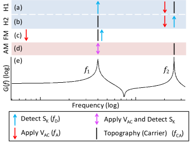
Figure 1: In H-KPFM ($\blacksquare$ a,b) an alternating voltage is applied at a frequency $f_{2}-f_{1}$ (${\color[rgb]{1,0,0}\downarrow}$). The cantilever’s response is mixed with oscillation at the carrier frequency in order to be detected at one resonance (${{\color[rgb]{0,0.6875,1}\uparrow}}$). The carrier oscillation occurs at another resonance and is also used to maintain time-averaged distance to the surface ($\mid$). Likewise, in the sideband implementation of FM-KPFM ($\square$, c) a voltage is applied and the response detected at different frequencies: the alternating voltage is applied at $f_{A}\ll f_{1}$ and detected at $f_{1}+f_{A}$. In AM-KPFM ($\blacksquare$), the alternating voltage is applied at the same frequency at which the cantilever response is detected (${\color[rgb]{.86,.4,.95}\updownarrow}$). The magnitude of the cantilever transfer function $G(f)$ with each eigenmode modeled as a point-mass, is shown in (e).

In AM-KPFM, $S_{K}$ is detected at the same frequency as the applied $V_{AC}$ (${\color[rgb]{.86,.4,.95}\updownarrow}$ in figure 1), i.e. $f_{D}=f_{A}$ for AM-KPFM. Here we calculate the force above a conducting sample by modeling the tip-sample system as an metallic capacitor with energy $U=1/2CV^{2}$. The case for semiconductors is more complicated, but KPFM feedback operation is similar, and reduces to the metal case in the heavily-doped limitHudlet1995 . The force on the cantilever has components at frequencies DC, $f_{D}$, and $2f_{D}$. The vertical force on the cantilever at frequency $f_{D}$ is thenJacobs1997 :

$$F_{f_{D}}=-C^{\prime}V_{AC}(V_{K}+V_{0}),$$ (2)

where $C^{\prime}=\frac{dC}{dz}$. We assume that the motion of each cantilever eigenmode is purely along the $z$-axis so that the transfer function of the cantilever $G(f)$ relates the driving force on the tip to the oscillation amplitude $A_{f}$ of the cantilever:

$$A_{f_{D}} =G(f_{D})F_{f_{D}}.$$ (3)

The optical lever sensitivity $\gamma(f)$ relates the signal generated at the photodetector to the amplitude of cantilever oscillation, so that:

$$S_{\text{photo}} =\gamma(f_{D})A_{f_{D}},$$ (4)

$$=-\gamma(f_{D})G(f_{D})C^{\prime}V_{AC}(V_{K}+V_{0}).$$

The signal from the photodetector is recorded by a quadrature lock-in amplifier with relative phase $\phi_{D}$:

$$S_{LIA}^{i} =\text{Re}[-\gamma(f_{D})G(f_{D})C^{\prime}V_{AC}(V_{K}+V_{0})e^{i\phi_{D}}],$$ (5)

$$S_{LIA}^{q} =\text{Re}[-\gamma(f_{D})G(f_{D})C^{\prime}V_{AC}(V_{K}+V_{0})e^{i(\phi_{D}+\frac{\pi}{2})}],$$

where $S_{LIA}^{i}$ and $S_{LIA}^{q}$ are the in-phase and quadrature components of the signal, respectively, at the lock-in amplifier. The KPFM feedback loop operates on $S_{LIA}^{i}$, and when put in the form of equation 1 is:

$$S_{K} \equiv S_{LIA}^{i}=-\zeta_{AM}(V_{K}+V_{0}),$$ (6)

where the sensitivity of AM-KPFM is:

$$\zeta_{AM}=\text{Re}[\gamma(f_{D})G(f_{D})C^{\prime}V_{AC}e^{i\phi_{D}}].$$ (7)

The relative phase of the lock-in amplifier, $\phi_{D}$, is adjusted in order to maximize the sensitivity for all techniques.

Table 1: Example cantilever characteristics

Name	$f_{1}$ (kHz)	$k_{1}$ (N/m)	$Q_{1}$	$\gamma_{1}$ (V/nm)	$f_{2}$	$k_{2}$	$Q_{2}$	$\gamma_{2}$
HQ:CSC35/Pt-C ($\mu$masch)	130	5.0	230	0.030	810	88	440	0.070

In H-KPFM and FM-KPFM, the cantilever is shaken with amplitude $A_{CA}$ at the carrier frequency $f_{CA}$ by a non-electrostatic method (here, photothermally), $V_{AC}$ is applied at $f_{A}$, and the KPFM signal is detected at $f_{D}$ ($\mid$, ${\color[rgb]{1,0,0}\downarrow}$, and ${{\color[rgb]{0,0.6875,1}\uparrow}}$, respectively, in figure 1). The oscillation $A_{CA}$ is used for topography control in single-pass mode, but is also critical for the H-KPFM signal, and so must be present, even when lift mode is used. We assume that the cantilever position is well-approximated by the sinusoidal motion at $f_{CA}$ (figure 1), so that:

$$(z-\bar{z})= A_{CA}\cos(2\pi f_{CA}t+\phi_{CA}),$$ (8)

where $z$ is the instantaneous tip-sample separation, $\bar{z}$ is the time-averaged separation, $A_{CA}$ is the amplitude of the carrier oscillation, and $\phi_{CA}$ is the phase. Here we Taylor expand the tip-sample electrostatic force around its time-averaged height $\bar{z}$ so that the capacitive force on the cantilever isSugawara2012 :

$$F=\Bigg{[}C^{\prime}+C^{\prime\prime}A_{CA}\cos(2\pi f_{CA}t+\phi_{CA})\Bigg{]}$$

$$\times\frac{[V_{AC}\cos(2\pi f_{A}t+\phi_{A})+V_{K}+V_{0}]^{2}}{2}.$$ (9)

As in AM-KPFM, a term linear in $V_{AC}$ is used for the KPFM feedback, and there are three frequencies at which such a signal is generated: $f_{A}$, $f_{A}+f_{CA}$, and $|f_{A}-f_{CA}|$. The force at the first frequency, proportional to $C^{\prime}$, is used for AM-KPFM (see equation 2), while the forces at the second and third frequencies, each proportional to $C^{\prime\prime}$, are used for H-KPFM. Then, up to a phase shift, each force is:

$$F_{f_{D}}=-\frac{C^{{}^{\prime\prime}}A_{CA}}{2}V_{AC}(V_{K}+V_{0}).$$ (10)

Like Sugawara et al. Sugawara2012 , we choose $f_{D}=f_{A}+f_{CA}$. The case $f_{D}=|f_{A}-f_{CA}|$ results in an equivalent force. Then, as with AM-KPFM above, the signal used for H-KPFM feedback depends on the cantilever transfer function and the optical lever sensitivity at the detection frequency, so that the signal at the photodiode is, up to a phase shift:

$$S_{\text{photo}} =-\frac{\gamma(f_{D})G(f_{D})C^{{}^{\prime\prime}}A_{CA}}{2}V_{AC}(V_{K}+V_{0}).$$ (11)

Once the phase shift is included, the H-KPFM feedback signal is put in the form of equation 1 with sensitivity:

$$\zeta_{H}=\text{Re}\biggl{[}\frac{\gamma(f_{D})G(f_{D})A_{CA}}{2}C^{{}^{\prime\prime}}V_{AC}e^{i(\phi_{CA}+\phi_{A}+\phi_{D})}\biggr{]}.$$ (12)

Thus the sensitivity of H-KPFM differs from AM-KPFM both by it dependence on $C^{\prime\prime}$ instead of $C^{\prime}$ and by its dependence on the carrier oscillation amplitude $A_{CA}$. If it is necessary to scan far from the surface, $A_{CA}$ can be increased to enhance sensitivity. Note that FM-KPFM similarly depends on $A_{CA}$Zerweck2005 .

In H-KPFM, both the detection frequency, $f_{D}$ and the carrier oscillation frequency, $f_{CA}$, are free to be chosen, and once chosen, determine the frequency at which $V_{AC}$ is applied, $f_{A}$. Earlier works on H-KPFM considered the case $f_{CA}=f_{1}$, the first cantilever resonance, and $f_{D}=f_{2}$, the second cantilever resonanceSugawara2012 ; Ma2013 ; Ma2013a . In this article, this implementation is called "H2" for heterodyne amplified by the second cantilever resonance. Here the case $f_{CA}=f_{2}$, $f_{D}=f_{1}$ is also considered, for enhanced sensitivity, and we call it "H1" because $S_{K}$ is amplified by the first resonance.

II.2 Experimental Setup

All methods are implemented on a commercial AFM (Cypher, Asylum Research). The motion of a platinum-coated cantilever is measured with an optical lever employing a 860 nm laser and detected by a quad-photodiode. The optical lever sensitivity is determined for each eigenmode from amplitude vs. distance curves, and the spring constants are determined by fitting the cantilever’s thermal spectrum (table 1).

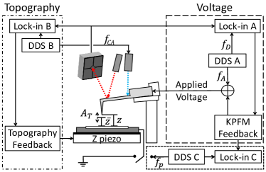
Figure 2: A feedback loop controls the separation between a photothermally driven cantilever and the sample through the cantilever’s oscillation amplitude by adjusting the sample height (left). A voltage $V_{AC}$ at frequency $f_{A}$ is added to $V_{K}$, the KPFM voltage, and applied to the probe. The cantilever oscillation at $f_{D}$ is then detected by lock-in amplifier B and used by a feedback loop to control the DC voltage applied to the cantilever (right). A third lock-in amplifier measures the response of $V_{K}$ to a perturbation in order to deduce the KPFM transfer function.

KPFM is implemented using two direct digital synthesizers (DDS), each paired with a lock-in amplifier (LIA). In particular, the cantilever is excited at $f_{CA}$ photothermally by DDS B (figure 2) for topography control. DDS A generates an AC voltage at frequency $f_{A}$ that is applied to the probe. LIA A detects the cantilever’s oscillation at $f_{D}$. The relative phases of signals from DDS A and B are maintained through the synchronization of the AFM’s internal clock. To measure the transfer function of the KPFM loop, DDS C is used to apply an AC voltage, $V_{p}$ to the substrate. LIA C detects the response of $V_{K}$ to the perturbation.

AM feedback is used for the topographical loop for all KPFM methods. In our earlier experimentGarrett2015 , an FM feedback loop controlled the tip-substrate distance while maintaining attractive-mode scanningGarcia1999 . Although FM topography feedback is adapted from the original implementation of H-KPFMSugawara2012 , it contains one major disadvantage: the frequency shift is a non-monotonic function of distanceGiessibl2003 and so the tip collides with the surface when its motion deviates too far from the topography setpoint. With AM topography control the feedback operates on a signal that is monotonic with distance, except at one bistability that can be avoidedGarcia1999 . When AM feedback is used for topography, small perturbations, that once destroyed probes, no longer affect scan stability.

The settings for the different KPFM techniques are chosen to realistically represent each technique’s capabilities and are similar to those of previous experimentsGlatzel2003 ; Zerweck2005 . FM-KPFM is implemented with sideband detectionZerweck2005 : $f_{CA}=f_{1}$ and $f_{D}=f_{1}+f_{A}$, and the modulation frequency $f_{A}=2$ kHz is maintained. For AM-KPFM, $V_{AC}$ is applied at $f_{1}$, and the topography loop operates at $f_{2}$. For H-KPFM, the H1 implementation uses $f_{CA}=f_{2}$ and $f_{D}=f_{1}$, while $f_{CA}=f_{1}$ and $f_{D}=f_{2}$ for H2 (see figure 1). For all methods, $V_{AC}=1\text{ V}.$

All scans are performed on a micron-sized flake of few-layer graphene (FLG) on boron doped silicon with a thin native oxide layer (15-25 Ohm-cm, Virginia Semiconductor), prepared by exfoliationNovoselov2004 . Both flakes of Highly Ordered Pyrolytic Graphite (HOPG) and FLG are observed with AFM. The HOPG is a few tens of nm tall and causes band bending in the Si surface potential at its edges but has negligible patch potentials. The FLG is $\approx$ 1 nm high and does not change the surface potential of Si around it but is covered with patch potentials. Because the FLG/Si boundary has less topography change, and a surface potential profile that is symmetric around the boundary, it is chosen for the following measurements.

II.3 Eliminating artifacts

Table 2: Common artifacts in Kelvin Probe Force Microscopy

Type	Example Source	H	FM	AM
Extraneous Signal ($S_{E}$)
Time-independent	AC inductive coupling, between $V_{AC}$ and piezo (figure 3)Barbet2014	-	-	$\times$
Periodic	Topographical oscillation detected in voltage bandwidth (figure 6i)	-	$\times$	-
Intermittent	Collision with surface	$\times$	$\times$	$\times$
Stray Capacitance	Long-range electrostatic force from cantilever Jacobs1997 ; Colchero2001 ; Ma2013	-	-	$\times$

Legend: $\times$ = large artifact, - = small artifact

Several artifacts originate from signals interfering with the Kelvin probe signal, $S_{K}$ Kalinin2000 ; Diesinger2008 ; Melin2011 ; Barbet2014 . Examples of such signals include AC coupling between $V_{AC}$ and a piezo in the cantilever holder (figure 3) or detection of the topography oscillation (at $f_{CA}$) within the lock-in amplifier (LIA) bandwidth (table 2). The resulting signal detected at the LIA contains both the desired signal, $S_{K}$, and an extraneous signal, $S_{E}$, and is given by:

$$S_{LIA}^{i}=S_{K}+S_{E}.$$ (13)

A setpoint, $S_{sp}$ for the voltage feedback loop is chosen to compensate for $S_{E}$ (above we assume $S_{E}=0$, and so a setpoint is not needed). When both $S_{E}$ and $S_{sp}$ are included, the Kelvin probe loop detects the voltage:

$$V_{K}=-V_{0}+V_{E},$$ (14)

which contains an extraneous voltage:

$$V_{E}=\frac{S_{E}-S_{sp}}{\zeta_{j}}.$$ (15)

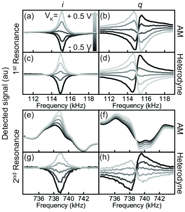
Figure 3: H-KPFM removes the distortion caused by AC coupling in the KPFM signal vs. detection frequency curves ($S^{i}_{LIA}$ vs $f_{D}$ and $S^{q}_{LIA}$ vs $f_{D}$). (a,b) At the first eigenmode, the in-phase ($i$) and quadrature ($q$) components of the AM-KPFM signal show little distortion, but (e,f) at the second eigenmode, distortion due to inductive AC coupling between the KPFM voltage and tip holder, which increases with frequency, is observed. (c,d,g,h) Heterodyne excitation generates no distortion. The KPFM voltage applied to the tip, $V_{K}$, is sampled at values above and below the contact potential difference. Similar measurements were used to detect AC coupling in Diesinger2008 .

The topography is imprinted on $V_{K}$ through the height-dependence of $\zeta_{j}$, the sensitivity from equation 1, which complicates attempts to remove the artifact in post-processingBarbet2014 .

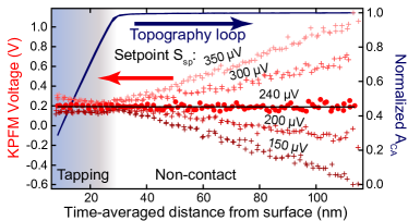
Figure 4: The setpoint of the KPFM feedback loop is adjusted to minimize the height-dependence of the KPFM voltage, $V_{K}$. Here the setpoint is swept from 150 to 350 $\mu$V over several approaches. The center curve (240 $\mu$V, $\color[rgb]{1,0,0}\bullet$) shows a distance dependence of only 0.03 mV/nm. The dark blue curve indicates the topographical oscillation amplitude normalized to its value far from the surface.

Conversely, the height dependence of $V_{E}$ can also be used to identify $S_{E}$. If $S_{E}$ is small enough and does not vary in time, $S_{sp}$ can be chosen so that the numerator of equation 15 vanishes. In this paper, the height dependence of $V_{K}$ is used to choose $S_{sp}$. If a sample has uniform surface potential, then:

$$\frac{dV_{K}}{d\bar{z}}=\frac{dV_{E}}{d\bar{z}}=\frac{S_{sp}-S_{E}}{\zeta_{j}^{2}}\frac{d\zeta_{j}}{d\bar{z}}.$$ (16)

If $dV_{K}/d\bar{z}\approx 0$, then $S_{sp}\approx S_{E}$, as $d\zeta_{j}/d\bar{z}$ does not vanish.

To minimize $V_{E}$, the KPFM feedback setpoint, $S_{sp}$, is varied over a range of 200 $\mu$V, and a $V_{K}$ vs. height curve is recorded for each $S_{sp}$ (figure 4). For most $S_{sp}$, the measured $V_{K}$ does depend on height, indicating that $S_{sp}\neq S_{E}$. The variation amongst the curves decreases when the tip-sample separation is reduced (until intermittent contact with the sample begins at $\approx$ 20 nm). The setpoint with the least distance dependence (240 $\mu$V), is maintained for the KPFM scans. The offset originates at the output of the low-pass filter on the lock-in amplifier for our setup, and it varies slightly from day to day, so the calibration must be repeated for every set of measurements.

III Resolutions

The temporal, voltage, and spatial resolutions of the different KPFM implementations are compared through several tests, the results of which are summarized in table 3.

III.1 Time Resolution

H-KPFM achieves fast time resolution by avoiding several artifacts that limit speed of the other KPFM techniques (Table 2). Because several limits on KPFM time resolution are proportional to $f_{D}$, such as the bandwidth of a cantilever resonance ($f_{D}/2Q$) and the Nyquist frequency ($f_{D}/2$), higher resonant frequencies are expected to increase bandwidth. However, for AM-KPFM, higher frequencies also increase the AC couplingBarbet2014 (figure 3). AC coupling does not affect H-KPFM or FM-KPFM as significantly because the applied and detected signals are at different frequencies. Consequently, H-KPFM can employ cantilevers with higher resonant frequencies than AM-KPFM. This limitation of AM-KPFM is due to the drive piezo that is present in most cantilever holders. Additional circuitry can mitigate this artifactDiesinger2008 ; Melin2011 ; Polak2014 , but typically the circuitry must be custom-made.

On the other hand, the artifact that limits FM-KPFM scan speed is fundamental to its operation. In both H- and FM-KPFM, carrier and KPFM signals must be present at the same time. If $A_{CA}=0$, then $S_{K}$ vanishes, even in lift mode (equation 11, Zerweck2005 ). FM-KPFM scan speed is limited by a periodic $S_{E}$ imprinted on the KPFM signal because the two signals, at $f_{D}$ and $f_{CA}$, are so close in frequency space. Then the extraneous signal is estimated by considering how the cantilever oscillation $A_{CA}$ at $f_{CA}$ is detected by a lock-in amplifier with reference signal at $f_{D}$. When the signal is input into equation 15, the extraneous voltage is:

$$V_{E}^{CA}=\frac{\gamma(f_{CA})A_{CA}}{\zeta_{j}}\text{Re}\Bigg{[}\frac{e^{i(2\pi f_{A}t)}}{1+if_{A}/B}\Bigg{]},$$ (17)

where $B$ is the bandwidth of the LIA’s low-pass filter, and we set $S_{sp}=0$ for simplicity. In typical KPFM operation, the prefactor, $\frac{\gamma(f_{CA})A_{CA}}{\zeta_{j}}$, is large compared to the surface voltage contrast being measured. To reduce $V_{E}^{CA}$ then, $B$ must be chosen so that $B\ll f_{A}$. For H-KPFM $f_{A}>$100 kHz, so the bound on $B$ is large. FM-KPFM, however, typically works with $f_{A}\approx 1-3$ kHz, which limits $B$. $V_{E}^{CA}$ decreases with increasing $f_{A}$, which can be used to increase the available bandwidth even though it concurrently decreases the sensitivity because $|G(f_{1}+f_{A})|$, which is proportional to the sensitivity, decreases with increasing $f_{A}$. Note also that $V_{E}^{CA}$ is periodic in time, and so it cannot be mitigated by varying the KPFM feedback loop setpoint.

Previous measurements of time resolution either investigate the KPFM feedback loop response to a periodic voltage applied to the setpointZerweck2005 , or substrate Diesinger2010 , or how quickly a well-characterized sample can be scanned while retaining KPFM contrastSinensky2007 . Here the former method is used to estimate the cut-off frequency, $f_{c}$, which is defined as the frequency at which the KPFM loop response has dropped to $\approx 71\%$ of the low-frequency response (-3 dB). In table 3, the cut-off time, $t_{c}=1/f_{c}$, is listed instead, so that smaller values indicate a better resolution.

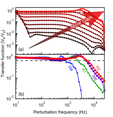
Figure 5: The transfer functions for the different KPFM methods are measured by applying a periodic voltage perturbation to the substrate and recording the response of the KPFM loop. (a) The transfer function of a H-KPFM voltage feedback loop increases and becomes more uniform as the gain is increased (H2 implementation). The proportional gain is increased 3 orders of magnitude, and overshoot is constrained to $\frac{V_{K}}{V_{p}}\leq 1.2$. A dashed line indicates the -3 db point used to calculate the cut-off frequency, $f_{c}$. (b) The cut-off frequency depends strongly on the method used, varying by almost an order of magnitude. The gain for each of the methods is chosen by the same optimization procedure.

The reported time resolutions of AM-KPFM typically exceed those of FM-KPFM, even though the specific resolution depends on both the cantilever and atomic force microscope used. Of the references discussed here, a few optimize temporal resolution for their AFMsSinensky2007 ; Diesinger2010 . For the others, the speeds cited are typical of an imaging method rather than the outcome of an optimization procedure. Diesinger et al.Diesinger2010 report an implementation of AM-KPFM that achieves $f_{c}\approx 200$ Hz, limited by the analog-digital conversion of the KPFM loop. In air, Sinensky and Belcher demonstrate that AM-KPFM can maintain some voltage contrast at scan speeds up to $1,172\text{ }\mu\text{m s}^{-1}$, by scanning 2-$\mu$m wide stripes of DNASinensky2007 . In the language used here, that corresponds to $f_{c}\approx 1.2$ kHz. FM-KPFM is reported to operate with similar speed when either in the sideband ($f_{c}\approx 35$ Hz) or phase locked loop ($f_{c}\approx 30$ Hz) is used, even though the sources of speed limitation are dissimilarZerweck2005 ; Diesinger2014 . Recent improvements to the KPFM feedback increase the cut-off frequency to 100 Hz with a larger modulation frequency (4 kHz)Wagner2015a . Reported open-loop FM-KPFM scan speeds include $0.85$ $\mu$m$s^{-1}$ (or 5 min per (500 nm)², 256$\times$256 pixel scan, trace and retrace)Borgani2014a and $1.3$ $\mu$m$s^{-1}$(or 3 min per (450 nm)², 256$\times$256 pixel scan, trace and retrace)Takeuchi2007 .

To measure the closed loop transfer function of each KPFM method, an AC voltage ($V_{p}=1$ V at perturbation frequency $f_{p}$) is applied to the substrate by a third DDS, while the cantilever height is maintained at the surface by a topographical feedback loop, with $A_{CA}\approx 8$ nm. The KPFM loop tracks the voltage, and $V_{K}(f_{p})$ is detected by a third lock-in amplifier. The frequency is swept from $f_{p}$ = 10 Hz to 25 kHz. The proportional gain of the control loop is increased until the bandwidth stops increasing, and the integral gain is then increased until the transfer function is flat across its bandwidth (figure 5). The cutoff frequencies for H2, H1, and AM are $5.3,2.3,$ and $5.0$ kHz, respectively (table 3). By further optimizing the feedback loops the bandwidth might be increasedDiesinger2010 ; Bechhoefer2005 ; Wagner2015a .

The measurement of the FM-KPFM transfer function is complicated by the presence of the topological feedback signal near the KPFM signal, which causes $V_{K}$ to include an extraneous, rapidly oscillating voltage (see equation 17). The separation between the KPFM signal and the interfering topography signal is equal to the $f_{A}$ of FM-KPFM, which here is 2 kHz, quite typical for FM-KPFMGlatzel2003 ; Zerweck2005 . First the transfer function is measured with only the lock-in amplifier’s own low-pass filter, but the extraneous voltage is so large that it overwhelms the signal until the frequency of the low-pass filter is decreased to 700 Hz, giving $f_{c}\approx 400$ Hz. However, the extraneous voltage imprinted by the topography signal remains $\approx 400$ mV, prohibitively large for practical measurements. Second, a notch filter is placed on the lock-in amplifier at $f_{A}$ (2 kHz) in order to further mitigate $V_{E}^{CA}$. The notch filter both decreases $V_{E}^{CA}$, and also allows the filter on the lock-in amplifier to be increased to 1 kHz. In this configuration the cutoff frequency of FM-KFPM is determined to be $f_{c}\approx 820$ Hz. It is worth noting that the measured bandwidths appear to exceed the bandwidth of the cantilever resonances, $f_{i}/2Q_{i}$. It is possible that the feedback of closed-loop methods flattens the transfer function analogously to the way the transfer function of an operational amplifier is flattened by placing a resistor across itBechhoefer2005 ; however, further investigations are warranted.

To investigate how $f_{c}$ translates into imaging speed, a few-layer graphene (FLG) flake is scanned with H- and FM-KPFM while the line scan speed is increased from 1 Hz to 79 Hz, over a 1$\times$1 $\mu$m area with 256$\times$256 pixels with $A_{CA}$ = 16 nm (figure 6). By 4 Hz (48 s per frame), FM-KPFM shows stripes. To investigate the cause of these stripes, the FLG is imaged without the aforementioned notch filter at 2 kHz. At 8 Hz, the amplitude of the stripes is $<0.3$ V with the notch filter, but rises to $>1.5$ V when the notch filter is removed. Thus the signal $V_{E}^{CA}$ does contribute to the stripe artifact, although the details of the feedback loop likely influence the stripes as well. At higher frequencies, the FM feedback loop oscillates wildly near the edges of the FLG.

With H-KPFM, on the other hand, clear contrast is maintained up to 16 Hz (16 s per frame), and at higher frequencies some contrast is maintained. However, the topographical feedback loop stops tracking the surface, and topographical inconsistency affects the potential image. At 79 Hz, patches on the graphene flake are no longer visible. A similar limitation due to topographical feedback loop speed is reported in Sinensky2007 .

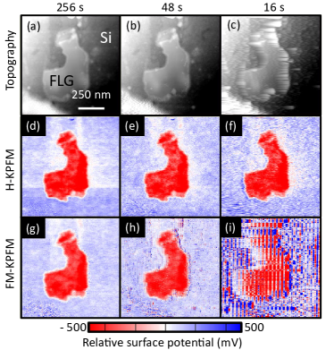
Figure 6: Images show the affect of increasing scan speed. (a-c) Topography images of the few layer graphene (FLG) become blurred. (d-f) H-KPFM allows the potential of FLG to be imaged with increasing speed and minimal distortion. (g-i) The topography oscillation is imprinted on the potential image when the bandwidth is increased if FM-KPFM is used. Topography scanning may be the primary speed limit. The height of the FLG is $\approx 2$ nm. All scans are 256$\times$256 pixels.

Table 3: Resolutions that characterize KPFM

Resolution	Figure of Merit	Definition	H2	H1	FM	AM	(units)
Time*	$t_{c}=1/f_{c}$	Closed-loop 3 dB cut-off timeDiesinger2010	0.19	0.43	1.2	0.20	ms
Voltage**	$V_{m}$	$V=V_{K}+V_{0}$ for which signal = noiseNonnenmacher1991	73	41	96	2.0	mV
Space**	$l_{10-90}$	Distance from boundary over which voltage	45	42	49	68	nm
		changes from 10% to 90% Zerweck2005

*At $A_{CA}=8$ nm, $V_{AC}=1$, $V_{p}=1$ V, and at the surface, with topographical feedback on

*At $A_{CA}=8$ nm, Bandwidth = 200 Hz, $V_{AC}$=1 V, and lift height 11 nm

III.2 Voltage Resolution

III.2.1 Accuracy

Whereas the tip apex detects the potential directly beneath it, the inclusion of stray capacitance from the cantilever results in surface potential spatially averaged over many microns (about the width of the cantilever)Jacobs1997 ; Koley2001 ; Colchero2001 ; Ma2013 . The unknown and varying relative capacitances of the tip apex and cantilever limit AM-KPFM to qualitative contrast in most conditionsJacobs1997 ; Colchero2001 . Both H-KPFM and FM-KFPM mitigate the stray capacitance effect through their dependence on $C^{\prime\prime}$ rather than $C^{\prime}$Glatzel2003 ; Ma2013 . Here the stray capacitance must be assessed in order to understand the relation between the measured potential sensitivity and the ability to actually distinguish between two nanoscale objects.

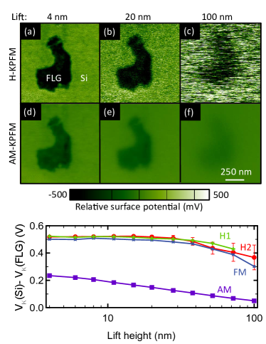
Figure 7: The voltage contrast between a few layer graphene (FLG) flake and Si substrate reveals the stray capacitance effect. (a-c) The voltage contrast between (few-layer) graphene and silicon changes little as the probe height increases from 4 to 100 nm for H-KPFM. (d-f) However, for AM-KPFM, the contrast at 100 nm differs by a factor of five from that at 4 nm. (g) A comparison between the four different KPFM methods shows that methods that depend on $C^{\prime\prime}$ more accurately represent the potential contrast than AM-KPFM, which depends on $C^{\prime}$.

The capacitance of tip and cantilever changes with tip-sample separation, and consequently, so does the measured average voltage contrast between the FLG flake and Si substrate, $\Delta V$. The correspondence between the actual and measured potentials is tested by observing the change of $\Delta V$ with lift height, akin to Spadafora2011 . At closest approach the tip apex capacitance dominates. As the tip-sample separation is increased, $\Delta V$ changes little until the proportion of capacitance due to the apex decreases to a value comparable to the cantilever capacitance contribution. The criterion of $\frac{d\Delta V}{d\bar{z}}\approx 0$ near the surface is adopted to ensure that the apex contribution dominates. In the limit of large lift height, the cantilever contribution dominates, and no potential contrast is observed. The potential contrast is estimated for each height by calculating the difference between the average potential inside the FLG/silicon boundary (figure 11e) and the average potential outside.

The contrast between Si and FLG changes little for H- and FM-KPFM, as the cantilever lift height is varied (figure 7a-c,g). On the other hand, the AM-KPFM detected voltage contrast changes by a factor of five as the lift height is decreased from 100 to 4 nm (figure 7d-f,g). Thus the average potential contrast measured with $C^{\prime\prime}$ methods is more accurate than the contrast measured by AM-KPFM.

III.2.2 Minimum detectable voltage

The minimum detectable voltage, $V_{m}$, is the tip-sample voltage difference at which the signal is equal to the noiseNonnenmacher1991 ; Giessibl2003 ; Sugawara2012 ; Ma2013a . Here $N(B)$ is the noise power in the signal $S^{i}_{LIA}$ within the bandwidth $B$. The minimum detectable voltage for any KPFM method is:

$$V_{m}=\frac{\sqrt{N(B)}}{\zeta_{j}}.$$ (18)

Note that $N(B)$ increases as the bandwidth increases. Thus increasing temporal resolution restricts voltage resolution.

The sources of noise in an AFM can be divided into three categoriesLabuda2012b . The first, detection noise, includes angular fluctuations of the light beam and optical shot noise. The second, displacement noise, includes the reaction of the topography feedback loop to perturbations, such as 60 Hz line noise or the voltages applied in KPFM. The third, force noise, includes Brownian motion and stresses caused by light optical intensity fluctuations. Because $f_{D}$ is near a resonance in H-KPFM, we assume Brownian motion is the dominant force noise. In this limit, the total noise in the signal is:

$$N(B) =\frac{1}{2}\int^{B}_{-B}\bigg{[}\frac{2\gamma_{i}^{2}k_{i}k_{B}T}{\pi f_{i}Q_{i}}|G(f_{i}+f)|^{2}$$ (19)

$$+n^{2}_{\text{det}}(f)+n^{2}_{\text{dis}}(f)\bigg{]}df,$$

where the first term in the brackets represents the noise due to Brownian motion of the cantileverHeer1972 , $k_{B}$ is Boltzmann’s constant, $T$ is temperature, $n_{\text{det}}$ is the detection noise amplitude spectral density (which is nearly constant over the integral), and $n_{\text{dis}}$ is displacement noise amplitude spectral density (which depends on the specifics of KPFM operation). If we consider only the Brownian motion of the cantilever, and assume the detection bandwidth $B$ is less than the bandwidth of the cantilever ($B<f_{i}/2Q_{i}$), then the integral in equation 19 can be computed analytically:

$$N(B) \approx\frac{\gamma_{i}^{2}k_{B}T}{\pi k_{i}}\text{arctan}\bigg{(}\frac{2Q_{i}B}{f_{i}}\bigg{)},$$ (20)

yielding the same noise as used in previous calculations of $V_{m}$, in the limit of small $B$Nonnenmacher1991 .

To understand how cantilever characteristics affect the minimum detectable voltage, each eigenmode of $G(f)$ is modeled as a point mass harmonic oscillatorMelcher2007 . Then the minimum detectable voltage becomes:

$$V_{m,\textrm{H}} =\frac{2\sqrt{2k_{B}T}}{\sqrt{\pi}A_{CA}V_{AC}C^{\prime\prime}}\sqrt{k_{i}\text{arctan}\bigg{(}\frac{2Q_{i}B}{f_{i}}\bigg{)}}.$$ (21)

Conversely, if the dominant noise source is broadband detector noise (e.g. off resonance), then $N(B)\approx n_{\text{det}}^{2}B$. The minimum detectable voltage when detector noise dominates is:

$$V_{m,\textrm{H}}=\frac{2n_{\text{det}}\sqrt{B}}{A_{CA}V_{AC}C^{\prime\prime}}\frac{1}{|G(f_{D})|\gamma(f_{D})}.$$ (22)

Note that the optical lever sensitivity depends on the eigenmode excited (a cantilever bends more for the same $z$ displacement if excited at higher eigenmodesButt1995 ).

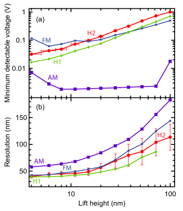
Figure 8: The (a) minimum detectable voltage and (b) 10-90 resolution both increase with lift height, for all methods. The data plotted here are for cantilever topographical oscillation of $A_{CA}=8$ nm. Both heterodyne methods achieve resolutions similar to FM-KFPM.

The minimum detectable voltage, $V_{m}$ is experimentally determined by measuring the signals at the lock-in amplifier, $S_{LIA}^{i}$ and $S_{LIA}^{q}$ (equation 5), with the feedback loop open. The detection phase, $\phi_{D}$, is swept from -180^∘ to 180^∘ at $V_{K}$ = -1, -0.3, 0.3, and 1 V. For each $\phi_{D}$, the sensitivity $\zeta_{j}$ is determined by fitting $S_{LIA}^{i}$ vs $(V_{K}+V_{0})$ to a line, the slope of which is $\zeta_{j}$ (equation 1). Calculating $\zeta_{j}$ for several $\phi_{D}$, allows us to account for a small systematic offset on the output of the LIA, and to determine the $\phi_{D}$ that maximizes $\zeta_{j}$. The noise at the output of the LIA is sampled at 5 kHz, and the calculations here consider the noise within a bandwidth of 200 Hz. Then equation 18 is used to calculate $V_{m}$.

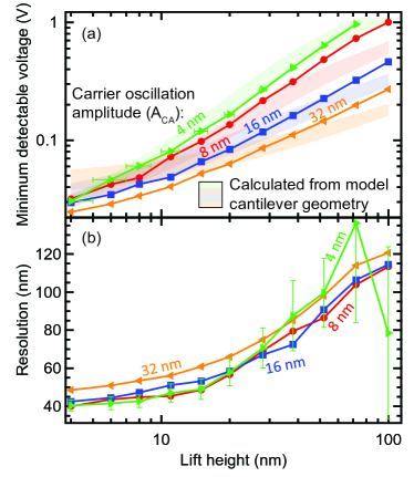
Figure 9: With H-KPFM in the H2 implementation, (a) the minimum detectable voltage, $V_{m}$, and (b) the 10-90 resolution, $l_{10-90}$, both increase with lift height. Larger shake amplitude, $A_{CA}$, decreases $V_{m}$, but no effect on resolution is found above the noise level as a function of $A_{CA}$. A cantilever model is used to calculate expected $V_{m}$ (shaded regions).

The lift-height dependence of $V_{m}$ for FM- and H-KPFM with different heights is measured. For each lift height, a force curve is used to set the position at the chosen lift height, where the probe is held for the duration of the $V_{m}$ measurement. As the separation is increased, $V_{m}$ increases, for all implementations (figure 8a). AM-KPFM has the smallest minimum detectable voltage; however, the small $V_{m}$ is a consequence of the stray capacitance of the cantilever, which causes potential contrast to only be qualitative, and limits spatial resolutionJacobs1997 ; Zerweck2005 . Within H2, $V_{m}$ increases more quickly with lift height for smaller $A_{CA}$ (figure 9a). In addition, $V_{m}$ is calculated from a model cantilever geometryColchero2001 combined with noise from equation 20 for the cantilever described in table 1, where the tip radius and opening angle are the only free parameters. A tip radius of $16\pm 2$ nm with an opening angle of $40\pm 5^{\circ}$ is found to approximate the $A_{CA}=4$ nm data. The calculated $V_{m}$ for this geometry, for all $A_{CA}$ are plotted in figure 9.

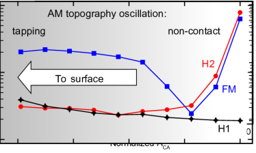
Figure 10: The minimum detectable voltage changes as a function of the normalized $A_{CA}$, which decreases as the probe moves closer to the surface (as in figure 4). A smaller setpoint moves the cantilever closer to the surface. Far from the surface H2 and FM-KFPM have similar $V_{m}$, but it becomes much greater for FM-KPFM nearer the surface, where the noise increases. The H1 method uses a different eigenmode for topography, and does not have the steep increase in $V_{m}$. The gradient from dark to light represents the change from tapping mode to a non-contact mode as the topography setpoint is increased and the probe is lifted from the surface.

Similarly, we measure $V_{m}$ while in tapping mode, as the topographical setpoint is gradually decreased. The noise in both H-KPFM implementations increases slowly as the setpoint is decreased, but the noise density in FM-KPFM increases rapidly, so that close to the surface, $V_{m}$ for FM-KPFM is about an order of magnitude larger (figure 10). Because the noise does not increase as rapidly for H1, the source of the noise is not solely due to using the first resonance for KPFM detection. Likewise, because the rapid noise increase is not seen in H2, the source of the extra noise is not solely due to which resonance is used for topography control. Thus, we suspect that the rapid increase in noise when FM-KPFM approaches the surface is due to signal detection ($f_{D}$) and topography control ($f_{CA}$) utilizing the same eigenmode.

III.3 Spatial resolution

Determining the spatial resolution of KPFM typically involves observing potential change around a boundary. Jacobs et al. showed that the boundary between two micron-scale objects allows for a clear empirical definition of spatial resolution and calculated a 25-75 resolution, i.e. the distance over which 50% of the total observed voltage change occurred, as a function of lift heightJacobs1997 ; Jacobs1998 ; McMurray2002 . Zerweck et al. similarly calculate a 10-90 resolutionZerweck2005 . An equation for the resolution from a point probe is derived in McMurray2002 . Others have sought information about the resolution by comparing the boundaries to particular functions, such as arctangentMcMurray2002 or Boltzmann functionsLiscio2006 .

Here we estimate a 10-90 resolution, $l_{10\text{-}90}$, by fitting the measured potential as a function of distance from the boundary to a hyperbolic tangent (figure 11). The theoretically expected form of the measured potential near the boundary is very nearly a tanh within the proximity force approximation, as shown in Appendix B. For large lift heights ($>20$ nm), the resolution is large enough to prevent $V_{K}$ from reaching its asymptotic value over the scan size, which necessitates the use of a fit. The noise inherent in KPFM is overcome by averaging around the boundary. The equation of the hyperbolic tangent fit to the boundary is:

$$\overline{V_{K}}(x)=(V_{b}\tanh\big{[}\text{ln}(9)(x-x_{0})/l_{10\text{-}90}\big{]}+c)/2,$$ (23)

where $V_{b}$ is the potential change across the boundary, $\overline{V_{K}}(x)$ is the average measured $V_{K}$ a distance $x$ from the boundary, $x_{0}$ is the center of the boundary, and $l_{10\text{-}90}$ is the 10-90 resolution. This fit gives the empirical spatial resolution. In order to determine whether or not the measured potential on either side of the boundary corresponds to the actual potential difference, one must supplement this data with either theoryZerweck2005 or knowledge of the accuracy of the detected voltage (as in figure 7).

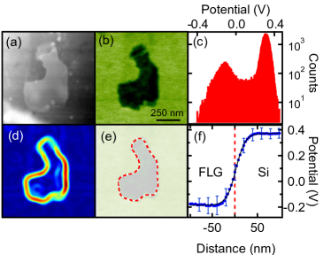
Figure 11: Few layer graphene on silicon shows (a) height contrast and (b) significant voltage contrast. (c) A histogram of the KPFM dat shows that the potential distribution is bimodal. (d,e) A watershed algorithm is applied to gradient magnitude of the potential image (d) in order to calculate the boundary (e, $\mathbf{---}$). (f) Voltages are summed as a function of the distance from the boundary ($\bullet$) and fit to a tanh function (black solid line), from which the 10-90 resolution is deduced.

Regions of few layer graphene and silicon are identified by watershed segmentationGonzalez2004 . First, the image is median filtered in order to mitigate the effect of noise on the algorithm, and the trace and retrace are averaged. Second, the gradient magnitude of the resultant potential image is calculated with a Sobel algorithmGonzalez2004 . Third, points of lowest and highest potential across the image are marked. Fourth, the watershed algorithm is applied with the two marked points forming the origin of each basin (figure 11).

Once the image is divided into two components, we plot the potential of the unaltered measurement as a function of the distance from the estimated boundary, and fit the resulting curve to an tanh function (figure 11e,f). The 10-90 resolution, $l_{10\text{-}90}$, is then extracted from the fit.

For all KPFM methods used, $l_{10\text{-}90}$ increases with lift height (figures 8,9b), as observed before with AM-KPFMJacobs1997 . Both implementations of H-KPFM and FM-KPFM achieve better spatial resolution than AM-KPFM, at all heights, but the error is too large to discern a difference between the former three. However, when the resolution approaches the length of the few layer graphene, or when the minimum detectable voltage reaches the contrast between the objects, the error grows large. Finding a longer, straighter boundary to measure, with larger contrast, could aid in future measurements of resolution at larger lift heights.

IV Conclusion

In this paper, we explore the versatility of H-KPFM and uncover its beneficial characteristics, the most prominent of which is its speed. The H1 implementation improves the minimum detectable voltage by $\approx 80\%$ relative to the original implementation. Further studies into the technique of H-KPFM should investigate the effect of roughness, the effect of eigenmode shape (reportedly an issue with the simpler AM-KPFMSatzinger2012 ), and how to incorporate better control techniques for potential estimation (e.g. Wagner2015a ) and tracking of the surface(e.g. Ahmad2014 ), which now limits KPFM scan speed. Cantilevers could be designed specifically for H-KPFMSadewasser2006 to reduce the difference between the spring constants of the first and second eigenmodes, which would improve the sensitivity of H-KPFM. Likewise, cantilever resonance frequencies could be chosen to enable open-loop H-KPFMCollins2013 .

Heterodyne KPFM improves upon the time resolution of FM-KPFM. Rates of several frames per minute are achieved. Its speed is not limited by AC coupling or bandwidth overlap, and so with appropriate cantilevers it will operate even faster. It also improves upon the spatial resolution of AM-KPFM. These new implementations of H-KPFM will facilitate fast and accurate measurements of nanoscale potential dynamics.

V Acknowledgements

We thank Asylum Research for technical advice, in particular Anil Gannepalli. We thank Tao Gong, Beth Tennyson, and Marina Leite for insightful conversations about KPFM and for challenging us with difficult-to-scan samples, and Dakang Ma and David Somers for critical readings of this article. We thank the University of Maryland for financial support.

Appendix A Table of Variables

Variable	Description	Equations
$S_{K}$	KPFM signal	1,6,13
$V_{K}$,$V^{C^{(n+1)}}_{K}$	KPFM voltage, KPFM voltage near a boundary	1,2,4,5,6,9,10,11,14,16,27,29,30
$V_{0}$	Inherent contact potential difference	1,2,4,5,6,9,10,11,14
$\zeta_{j}$	Sensitivity of KPFM method $j$, where $j$ = AM, FM, or H	1,6,7,12,15,16,17,18
$f_{D}$	Frequency at which the KPFM signal is detected	2,5,12
$F_{f_{D}}$	Force on cantilever at detection frequency	2,3,10
$C$	Tip-sample capacitance	2,4,5,7,9,10,11,21,22
$V_{AC}$	Periodic voltage applied to cantilever	2,4,7,9,10,11,12,21,22
$A_{f_{D}}$	Amplitude of cantilever oscillation at $f_{D}$	3
$G(f)$	Transfer function of cantilever at frequency $f$	3,4,5,7,11,12,22
$S_{\text{photo}}$	KPFM signal at photodetector	4,11
$\gamma(f),\gamma_{i}$	Optical lever sensitivity of cantilever at frequency $f$ or eigenmode $i$	4,5,7,11,12,17,19,20
$S_{LIA}^{i}$,$S_{LIA}^{q}$	In-phase ($i$) and $\pi/2$-shifted ($q$) signals at lock-in	5,6,13
$\phi_{D}$	Phase of shift of lock-in amplifier	5,7,12
$z$, ($\bar{z}$)	Instantaneous (time-averaged) tip-sample separation	8,16,24,25,26,32,33
$F$	Capacitive force on cantilever	9,24,25
$t$	Time	8,17
$A_{CA}$	Amplitude of carrier oscillation, also used for topography feedback	8,9,10,11,12,17,21,22
$f_{CA}$	Frequency of carrier oscillation	8,9
$\phi_{CA}$	Phase of carrier oscillation	8,12
$f_{A}$	Frequency at which $V_{AC}$ is applied to the cantilever	9,17
$\phi_{A}$	Phase of applied voltage $V_{AC}$	9,12
$S_{E}$	Extraneous signal in KPFM feedback	13,15,16
$V_{E}{,V_{E}^{CA}}$	Extraneous voltage artifact	14,15,16,17
$S_{sp}$	KPFM feedback setpoint	15,16
$B$	Bandwidth of low-pass filter on lock-in amplifier	17,18,19,20,21,22
$V_{p}$	Voltage perturbation applied to plate
$f_{p}$	Frequency of voltage perturbations applied to plate
$t_{c}=1/f_{c}$	The cut-off time and the cut-off frequency
$V_{m}$	Minimum detectable voltage	18,21,22
$N(B)$	Noise power in detection bandwidth	18,19,20
$k_{i}$, $Q_{i}$, $f_{i}$	Spring constant, quality factor, or frequency of eigenmode $i$	19,20,21
$n_{\text{det}},n_{\text{dis}}$	Detection and displacement noise amplitude spectral densities	19,22
$V_{b}$	Surface voltage change across a boundary	23,27,28,29
$L\equiv x-x_{0}$	Distance from potential boundary	23,26,27,29,30
$l_{10-90}$,$l_{10-90}^{C^{(n+1)}}$	10-90 resolution, for method that depends on $C^{(n+1)}$	23,32,33
$R$	Tip radius	24,25,26,32,33
$V_{pl}(r,\phi)$, $V$	Surface potential of the plate, sphere in PFA	24,25,26

Appendix B An equation for spatial resolution

Above we discuss the spatial resolution of KPFM in terms of $l_{10\text{-}90}$, the 10-90 resolution, or the distance over which 80% of the voltage change across a boundary occurs. We determine $l_{10\text{-}90}$ by fitting $V_{K}(x)$, the potential measured across a boundary, to a hyperbolic tangent (equation 23).

Here, we use the proximity force approximation (PFA) for a sphere interacting with a plate to derive an analytic expression for $V_{K}(x)$ for both $C^{\prime}$ and $C^{\prime\prime}$ KPFM methods. Furthermore, we demonstrate that the tanh function approximates the form of $V_{K}(x)$ better than the arctan function in order to motivate our choices in the text. Finally, we estimate how $l_{10\text{-}90}$ changes with height and tip radius. We note that an equation for resolution exists in the large separation, small probe limitMcMurray2002 , but better resolution is achieved with small tip-sample separation, and so that is our focus here.

The PFA for the capacitive force of a sphere above a plate can be written asKim2010 :

$$F(z)=\frac{\epsilon_{0}}{2}\int_{0}^{2\pi}{d\phi}\int_{0}^{R}rdr\frac{(V-V_{pl}(r,\phi))^{2}}{(z+r^{2}/2R)^{2}},$$ (24)

where $R$ is the radius of the sphere, $V_{p}(r,\phi)$ is the potential of the plate at position $(r,\phi)$, and $V$ is the potential of the sphere (here assumed to be spatially uniform). The voltage applied to the probe that minimizes $n$th derivative of this force can be found by taking $n$ derivatives with respect to $z$ and one with respect to $V$,

$$\frac{\partial^{n+1}F(z)}{\partial V\partial z^{n}}=\frac{\partial}{\partial z^{n}}\Biggl{[}\epsilon_{0}\int_{0}^{2\pi}{d\phi}\int_{0}^{R}rdr\frac{V-V_{pl}(r,\phi)}{(z+r^{2}/2R)^{2}}\Biggr{]}.$$ (25)

At the Kelvin probe voltage, $V=V_{K}(x)$, for which the KPFM signal $S_{K}$ vanishes, equation 25 vanishes as well. Near a boundary, the potential of the plate is $V_{pl}(r,\phi)=V_{b}\Theta(\cos(\phi)+L/r)$, where $L=x-x_{0}$ is the distance between the location of the probe and the boundary and $\Theta$ is the Heaviside step function . The potential is $V_{b}$ for $r\cos(\phi)>-L$ and 0 otherwise. To simplify the calculation, we define the function $\Lambda(z,R,L)$:

$$\Lambda(z,R,L)=\int_{0}^{2\pi}{d\phi}\int_{0}^{R}rdr\frac{\Theta(\cos(\phi)+L/r)}{(z+r^{2}/2R)^{2}},$$ (26)

$$=R\left(\frac{2L\text{ arctan}\left(\sqrt{\frac{R^{2}-L^{2}}{L^{2}+2Rz}}\right)}{z\sqrt{L^{2}+2Rz}}+\frac{2R\text{ arccos}\left(-\frac{L}{R}\right)}{z(R+2z)}\right).$$

For a KPFM method with a signal proportional to the $(n+1)^{\text{th}}$ derivative of capacitance, the Kelvin probe voltage near a boundary is:

$$V^{C^{(n+1)}}_{K}(L)=V_{b}\frac{\Lambda^{(n)}}{2\Lambda^{(n)}|_{L=0}},$$ (27)

where $\Lambda^{(n)}=\frac{\partial^{n}\Lambda}{\partial z^{n}}$, and $C^{(n+1)}$ represents a method that depends on the $(n+1)^{\text{th}}$ derivative of capacitance. For example, for AM-KPFM, the signal of which is proportional to $C^{\prime}$, the Kelvin probe voltage is:

$$V^{C^{(1)}}_{K}(L)= V_{b}\bigg{[}\frac{1}{2}+\frac{\text{ arcsin}\left(\frac{L}{R}\right)}{\pi}$$

$$+\frac{L(2z+R)\text{ arctan}\left(\sqrt{\frac{R^{2}-L^{2}}{L^{2}+2zR}}\right)}{\pi R\sqrt{2zR+L^{2}}}\bigg{]}.$$ (28)

It must be noted that the PFA only considers the contribution of the tip apex to the KPFM signal. In AM-KPFM the dominant contribution to the signal comes from the cantilever. At a boundary, equation 28 will predict the shape of $V^{C^{(1)}}_{K}(x)$, but the $V_{b}$ coefficient will be much less than the potential difference across the boundary. AM-KPFM measures qualitative potential contrastJacobs1997 .

For the $C^{\prime\prime}$ methods (H- or FM-KPFM) the minimizing potential equation is more complicated, and so it has been plotted in figure 12a.

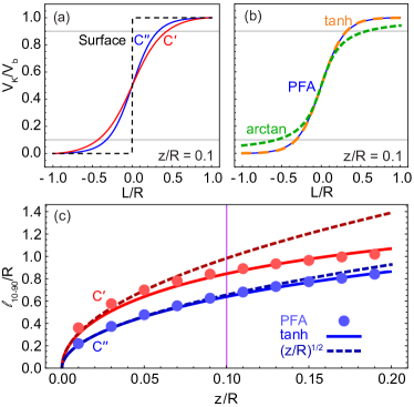
Figure 12: The normalized Kelvin probe voltage near a boundary in the proximity force approximation (PFA) is shown in (a) for both the AM-KPFM ($C^{\prime}$, red) and H- and FM-KPFM ($C^{\prime\prime}$, blue) variants. The dashed black line shows the normalized potential on the surface directly and two grey lines indicate the 10-90 potential change. (b) A tanh function (dashed orange) is a much better fit to the analytic expression (PFA) for the $C^{\prime\prime}$ method than an arctan function chosen in the same way (dashed green). (c) The 10-90 resolution predicted by a tanh function fit (solid) is compared to that calculated numerically by the exact PFA expression (${\color[rgb]{0,0,1}\bullet}$). At small z/R, the 10-90 resolution increases with separation $\propto\sqrt{z/R}$, and this approximate expression is plotted for both the $C^{\prime}$ and $C^{\prime\prime}$ methods (dashed). A purple line indicates the value of $z/R$ for which (a,b) are plotted.

To facilitate data analysis, a simpler function can be used to approximate equation 27. Both arctan and tanh functions have the desired behavior: monotonic, odd around $L=0$, and asymptotic to a constant as $L\rightarrow\infty$. The slope of $V^{C^{(n+1)}}_{K}(L)$ is steepest at $L=0$ and so fitting for small $L$ is most important. Arctan and tanh are used to approximate equation 27 by matching the first derivative of each function to our exact analytic expression:

$$V^{C^{(n+1)}}_{\text{tanh}}= V_{b}\frac{\tanh(2a^{C^{(n+1)}}L)+1}{2},$$ (29)

$$V^{C^{(n+1)}}_{\text{arctan}}= V_{b}\frac{\arctan(\pi a^{C^{(n+1)}}L)+\pi/2}{\pi},$$

where,

$$a^{C^{(n+1)}}= \frac{\partial V^{C^{(n+1)}}_{K}}{\partial L}\Bigg{|}_{L=0},$$ (30)

Both functions are plotted in figure 12b to visually depict how well each fits equation 27. The tanh fit follows the exact expression more closely than the arctan fit. The tanh fit can then be used to estimate $l_{10-90}$ as a function of z and R:

$$l_{10-90}^{C^{(n+1)}}= \frac{\text{ln}(9)}{2a^{C^{(n+1)}}}.$$ (31)

Which, for AM-KFPM is:

$$l_{10-90}^{C^{(1)}}= \frac{\pi\log(81)\sqrt{zR}}{2\sqrt{z/R}+\sqrt{2}(2z/R+1)\text{ arctan}\left(\sqrt{\frac{R}{2z}}\right)}.$$ (32)

The more complicated expression of $l_{10-90}^{C^{\prime\prime}}$ is plotted in figure 12c. Taylor expanding around $\sqrt{z/R}\approx 0$, the resolutions are:

$$\frac{l_{10-90}^{C^{(1)}}}{R}\approx\sqrt{2}\text{ ln}(9)\sqrt{\frac{z}{R}} \text{ (AM method)},$$ (33)

$$\frac{l_{10-90}^{C^{(2)}}}{R}\approx\frac{2}{3}\sqrt{2}\text{ ln}(9)\sqrt{\frac{z}{R}} \text{ (H-,FM- methods)}.$$

Jump-to-contact limits how small z can become, and consequently limits the possible spatial resolution. These approximations are also compared to the exact PFA result in figure 12c.

The resolutions calculated here are a lower bound on the resolution possible with KPFM because many components of the probe that would broaden the resolution are neglected. Though the electrostatic probe-surface force from the tip cone and cantilever have been calculated for uniform potentialHudlet1998 ; Colchero2001 , we are unaware of any analytic procedure to take into account variations of the surface potential. A procedure does exist to calculate the electrostatic force between a sphere and a plate with potential variationsBehunin2012a , but the KPFM probe geometry is only slightly better represented by such a model. Most importantly, these extra cases all reduce to the PFA near the surface, where the best spatial resolution is achieved.

References

- (1) Nonnenmacher M, O’Boyle M P and Wickramasinghe H K 1991 Appl. Phys. Lett. 58 2921
- (2) Nonnenmacher M, O’Boyle M and Wickramasinghe H K 1992 Ultramicroscopy 44 268–273
- (3) Weaver J M R and Abraham D W 1991 J. Vac. Sci. Technol. B 9 1559
- (4) Henning A K, Hochwitz T, Slinkman J, Never J, Hoffmann S, Kaszuba P and Daghlian C 1995 J. Appl. Phys. 77 1888
- (5) Kikukawa A, Hosaka S and Imura R 1995 Appl. Phys. Lett. 66 3510
- (6) Lü J, Delamarche E, Eng L, Bennewitz R, Meyer E and Güntherodt H J 1999 Langmuir 15 8184–8188
- (7) Reitzel N, Hassenkam T, Balashev K, Jensen T R, Howes P B, Kjaer K, Fechtenkötter A, Tchebotareva N, Ito S, Müllen K and Bjørnholm T 2001 Chem. Eur. J. 7 4894–4901
- (8) Gaillard N, Gros-Jean M, Mariolle D, Bertin F and Bsiesy A 2006 Appl. Phys. Lett. 89 154101
- (9) Sinensky A K and Belcher A M 2007 Nat. Nanotechnol. 2 653–659
- (10) Jacobs H O, Knapp H F, Müller S and Stemmer A 1997 Ultramicroscopy 69 39–49
- (11) Lee I, Lee J W, Stubna A and Greenbaum E 2000 J. Phys. Chem. B 104 2439–2443
- (12) Palermo V, Palma M and Samorì P 2006 Adv. Mater. 18 145–164
- (13) Colchero J, Gil A and Baró A M 2001 Phys. Rev. B 64 245403
- (14) Koley G, Spencer M G and Bhangale H R 2001 Appl. Phys. Lett. 79 545
- (15) Ma Z M, Kou L, Naitoh Y, Li Y J and Sugawara Y 2013 Nanotechnology 24 225701
- (16) Diesinger H, Deresmes D, Nys J P and Mélin T 2008 Ultramicroscopy 108 773–781
- (17) Mélin T, Barbet S, Diesinger H, Théron D and Deresmes D 2011 Rev. Sci. Instrum. 82 036101
- (18) Polak L, de Man S and Wijngaarden R J 2014 Rev. Sci. Instrum. 85 046111
- (19) Barbet S, Popoff M, Diesinger H, Deresmes D, Théron D and Mélin T 2014 J. Appl. Phys. 115 144313
- (20) Kitamura S and Iwatsuki M 1998 Appl. Phys. Lett. 72 3154
- (21) Glatzel T, Sadewasser S and Lux-Steiner M 2003 Appl. Surf. Sci. 210 84–89
- (22) Zerweck U, Loppacher C, Otto T, Grafström S and Eng L M 2005 Phys. Rev. B 71 125424
- (23) Panchal V, Pearce R, Yakimova R, Tzalenchuk A and Kazakova O 2013 Sci. Rep. 3 2597
- (24) Sommerhalter C, Matthes T W, Glatzel T, Jäger-Waldau A and Lux-Steiner M C 1999 Appl. Phys. Lett. 75 286
- (25) Sadewasser S, Glatzel T, Rusu M, Jäger-Waldau A and Lux-Steiner M C 2002 Appl. Phys. Lett. 80 2979
- (26) Leonenko Z, Gill S, Baoukina S, Monticelli L, Doehner J, Gunasekara L, Felderer F, Rodenstein M, Eng L M and Amrein M 2007 Biophys. J. 93 674–683
- (27) Sadewasser S, Glatzel T, Schuler S, Nishiwaki S, Kaigawa R and Lux-Steiner M 2003 Thin Solid Films 431-432 257–261
- (28) Zhang Y, Chen Q, Alivisatos A P and Salmeron M 2015 Nano Lett. 15 4657–4663
- (29) Mohn F, Gross L, Moll N and Meyer G 2012 Nat. Nanotechnol. 7 227–231
- (30) Gross L, Mohn F, Liljeroth P, Repp J, Giessibl F J and Meyer G 2009 Science 324 1428–1431
- (31) Coffey D C and Ginger D S 2006 Nat. Mater. 5 735–740
- (32) Murawski J, Graupner T, Milde P, Raupach R, Zerweck-Trogisch U and Eng L M 2015 J. Appl. Phys. 118 154302
- (33) Takeuchi O, Ohrai Y, Yoshida S and Shigekawa H 2007 Jpn. J. Appl. Phys. 46 5626–5630
- (34) Collins L, Kilpatrick J I, Weber S A L, Tselev A, Vlassiouk I V, Ivanov I N, Jesse S, Kalinin S V and Rodriguez B J 2013 Nanotechnology 24 475702
- (35) Borgani R, Forchheimer D, Bergqvist J, Thorén P A, Inganäs O and Haviland D B 2014 Appl. Phys. Lett. 105 143113
- (36) Moores B, Hane F, Eng L and Leonenko Z 2010 Ultramicroscopy 110 708–711
- (37) Tennyson E M, Garrett J L, Frantz J A, Myers J D, Bekele R Y, Sanghera J S, Munday J N and Leite M S 2015 Adv. Energy Mater. 5
- (38) Sengupta E, Domanski A L, Weber S A L, Untch M B, Butt H J, Sauermann T, Egelhaaf H J and Berger R 2011 J. Phys. Chem. C 115 19994–20001
- (39) Sugawara Y, Kou L, Ma Z, Kamijo T, Naitoh Y and Jun Li Y 2012 Appl. Phys. Lett. 100 223104
- (40) Wastl D S, Weymouth A J and Giessibl F J 2013 Phys. Rev. B 87 245415
- (41) Ma Z M, Mu J L, Tang J, Xue H, Zhang H, Xue C Y, Liu J and Li Y J 2013 Nanoscale Res. Lett. 8 532
- (42) Hudlet S, Saint Jean M, Roulet B, Berger J and Guthmann C 1995 J. Appl. Phys. 77 3308
- (43) Garrett J L, Somers D and Munday J N 2015 J. Phys. Condens. Matter 27 214012
- (44) García R and San Paulo A 1999 Phys. Rev. B 60 4961–4967
- (45) Giessibl F J 2003 Rev. Mod. Phys. 75 949–983
- (46) Novoselov K S, Geim A K, Morozov S V, Jiang D, Zhang Y, Dubonos S V, Grigorieva I V and Firsov A A 2004 Science 306 666–669
- (47) Kalinin S V and Bonnell D A 2000 Phys. Rev. B 62 419–430
- (48) Diesinger H, Deresmes D, Nys J P and Mélin T 2010 Ultramicroscopy 110 162–169
- (49) Diesinger H, Deresmes D and Mélin T 2014 Beilstein J. Nanotechnol. 5 1–18
- (50) Wagner T, Beyer H, Reissner P, Mensch P, Riel H, Gotsmann B and Stemmer A 2015 Beilstein J. Nanotechnol. 6 2193–2206
- (51) Bechhoefer J 2005 Rev. Mod. Phys. 77 783–836
- (52) Spadafora E J, Linares M, Nisa Yahya W Z, Lincker F, Demadrille R and Grevin B 2011 Appl. Phys. Lett. 99 233102
- (53) Labuda A, Bates J R and Grütter P H 2012 Nanotechnology 23 025503
- (54) Heer C V 1972 Statistical Mechanics, Kinetic Theory, and Stochastic Processes (New York: Academic Press, Inc.)
- (55) Melcher J, Hu S and Raman A 2007 Appl. Phys. Lett. 91 053101
- (56) Butt H J and Jaschke M 1995 Nanotechnology 6 1–7
- (57) Jacobs H O, Leuchtmann P, Homan O J and Stemmer A 1998 J. Appl. Phys. 84 1168
- (58) McMurray H N and Williams G 2002 J. Appl. Phys. 91 1673
- (59) Liscio A, Palermo V, Gentilini D, Nolde F, Müllen K and Samorì P 2006 Adv. Funct. Mater. 16 1407–1416
- (60) Gonzalez R C, Woods R E and Eddins S L 2004 Digital Image Processing Using MATLAB vol 1 (Pearson)
- (61) Satzinger K J, Brown K A and Westervelt R M 2012 J. Appl. Phys. 112 064510
- (62) Ahmad A, Schuh A and Rangelow I W 2014 Rev. Sci. Instrum. 85 103706
- (63) Sadewasser S, Villanueva G and Plaza J A 2006 Appl. Phys. Lett. 89 033106
- (64) Kim W J, Sushkov A O, Dalvit D A R and Lamoreaux S K 2010 Phys. Rev. A 81 022505
- (65) Hudlet S, Saint Jean M, Guthmann C and Berger J 1998 Eur. Phys. J. B 2 5–10
- (66) Behunin R O, Zeng Y, Dalvit D A R and Reynaud S 2012 Phys. Rev. A 86 052509