An extensive radial velocity survey toward NGC 6253

Abstract

The old and metal rich open cluster NGC 6253 was observed with the FLAMES multi-object spectrograph during an extensive radial velocity campaign monitoring 317 stars with a median of 15 epochs per object. All the targeted stars are located along the upper main sequence of the cluster between 14.8 $<$ V $<$ 16.5. Fifty nine stars are confirmed cluster members both by radial velocities and proper motions and do not show evidence of variability. We detected 45 variable stars among which 25 belong to NGC 6253. We were able to derive an orbital solution for 4 cluster members (and for 2 field stars) yielding minimum masses in between $\sim$90 M_J and $\sim$460 M_J and periods between 3 and 220 days. Simulations demonstrated that this survey was sensitive to objects down to 30 M_J at 10 days orbital periods with a detection efficiency equal to 50%. On the basis of these results we concluded that the observed frequency of binaries down to the hydrogen burning limit and up to 20 days orbital period is around (1.5$\pm$1.3)% in NGC 6253. The overall observed frequency of binaries around the sample of cluster stars is (13$\pm$3)%. The median radial velocity precision achieved by the GIRAFFE spectrograph in this magnitude range was around $\sim$240m$\rm\,s^{-1}$ ($\sim$180 m$\rm\,s^{-1}$ for UVES). Based on a limited follow-up analysis of 7 stars in our sample with the HARPS spectrograph we determined that a precision of 35 m $\rm s^{-1}$ can be reached in this magnitude range, offering the possibility to further extend the variability analysis into the substellar domain. Prospects are even more favourable once considering the upcoming ESPRESSO spectrograph at VLT.

1 Introduction

NGC 6253 ($\alpha_{2000}=16^{h}\,59^{m}\,05^{s},\delta_{2000}=-52^{\circ}\,42\arcmin\,30\arcsec,l=335\aas@@fstack{\circ}5,b=-6\aas@@fstack{\circ}3$) is an old and metal-rich open cluster located inside the solar ring and projected toward a rich Galactic stellar field in the direction of the Galactic center. The metal-rich nature of this cluster and its importance in the context of Galactic studies were early recognized in the seminal work of Bragaglia et al. (1997) and later on discussed by several other authors in the past (Piatti et al. 1998; Sagar, Munari, & de Boer 2001; Twarog, Anthony-Twarog & De Lee 2003; Anthony-Twarog, Twarog, & Mayer 2007; Carretta et al. 2000; Carretta, Bragaglia & Gratton 2007; Sestito et al. 2007; Anthony-Twarog et al. 2010). Novel chemical studies have been recently presented in Mikolaitis et al. (2012) where C,N,O abundances and carbon isotope ratios for four red clump stars of NGC 6253 were analyzed and in Cummings et al. (2012), focused on lithium abundance.

In the context of extrasolar planet searches NGC 6253 plays a major role. Given its high metallicity and the well known fact that the frequency of jupiter planets found around field stars is known to strongly correlate with metallicity (e.g. Gonzalez 1997; Santos et al. 2001; Santos et al. 2004; Fischer & Valenti 2005; Mortier et al. 2012) we may expect a large population of these objects to be present in this cluster, unless other evolutionary and environmental factors alter their formation histories.

Our previous efforts to detect this population and to better characterize cluster properties were presented in a sequence of works starting with Montalto et al. (2009, hereafter M09) where we delivered a photometric and astrometric catalog including proper motions membership probabilities. De Marchi et al. (2010) studied the photometric variability properties of cluster members and the surrounding field producing a catalog of 595 variables, 35 of which were proposed as cluster members. In Montalto et al. (2011, hereafter M11) we presented the results of a radial velocity survey conducted with the UVES/GIRAFFE spectrographs at VLT, mostly concentrated on the evolved portion of the color-magnitude diagram. In that work, we presented a follow-up analysis of three planetary candidates we found in our photometric studies and highlight the discovery of the first cluster double lined eclipsing binary system, located in the turn-off region (star 45368 in our catalog) which membership was confirmed both by proper motions and by radial velocities. We analyzed a sample of 139 stars in the cluster region concluding that 35 where likely cluster members and 12 likely close binary systems.

In Montalto et al (2012), we performed equivalent width analysis and derived Fe, Si, Ca, Ti, Cr and Ni abundances as well as abundance ratios of a main-sequence star, two red-clump stars and a blue straggler cluster members. For our main-sequence star, we obtained a metallicity of [Fe/H]=+0.26$\pm$0.11 (rms), whereas for the two giants we found that our metallicities were on average [Fe/H]=+0.19$\pm$0.13 (rms), lower than what was determined in previous studies (Sestito et al. 2007, [Fe/H]=+0.36$\pm$0.07 rms, Carretta et al. 2007, [Fe/H]=+0.46$\pm$0.03 rms).

NGC-6253 fundamental parameters are not yet firmly set. It is well known that the different calibrated photometries presented so far do not agree well, and that significant differences exist among them. The cluster age was set to 3.5 Gyr in M09 and the reddening to $E(B-V)$=0.15. These estimates were respectively the upper bound age and the lower bound reddening derived from isochrone fit so far, once compared with the other results in the literature. However recently Rozyczka et al. (2014) presented a detailed analysis of the eclipsing binary 45368 (renamed in their work V15). Their results indicate that the age of NGC 6253 should be comprised between 3.80 - 4.25 Gyr from the mass-radius diagram and should be even older (3.9 - 4.6 Gyr) from color-magnitude diagram (CMD) fitting. They also report a reddening equal to $E(B-V)$=0.113 mag, and therefore lower than our own value. The same authors presented in Kaluzny et al. (2014) the results of a novel photometric campaign in the cluster region, conducted with the 1.0m Swope Telescope in Las Campanas, focusing primarily on the bright portion of the CMD, in a domain only partially covered by our previous photometric surveys. Among a sample of 25 additional variables the authors detected three novel eclipsing binaries members of the cluster. The analysis of these objects will likely permit to reach more stringent constraints on cluster properties and to further complement the results obtained for 45368. It has been also demonstrated that theoretical models fail to accurately reproduce the observed CMD, particularly for evolved stars (M09, Anthony-Twarog 2010, Rozyczka et al. 2014).

In this work, we present the results of another extensive radial velocity campaign that was performed on this cluster in the past years. This survey superseeds by far both in number of monitored objects and in number of epochs the analysis presented in M11 and also the similar one discussed in Anthony-Twarog (2010). It represents a more ambitious effort to better characterize radial velocity variability among cluster members, and an important step toward the detection of low mass objects. The preparation of the observations presented in this work preceeded in time the photometric and astrometric analysis discussed in M11. Sample selection was based on the work of Twarog, Anthony-Twarog & De Lee (2003). The magnitude range of the sample stars is comprised in between 14.8$<$ V $<$16.5. All the targeted stars lie on the upper main sequence of NGC 6253.

In Section 2, we describe the observations we acquired. In Section 3, we discuss data reduction. In Section 4, we present the methods used to identify variables and in Section 5 our classification criteria. In Section 6, we describe the analysis of a sample of spectroscopic binaries. In Sec. 7, we compare our results with the ones obtained during previous surveys. In Section 8, we calculate the survey detection efficiency. Finally in Section 9, we summarize and conclude.

2 Observations

The observations described in this work have been acquired with FLAMES (Pasquini et al. 2002) and HARPS (Mayor, M. et al. 2003) spectrographs. FLAMES is the multi-object, intermediate and high resolution spectrograph of the VLT installed at the UT2 (Kueyen telescope), in Paranal, Chile. FLAMES is a complex system that feeds two different spectrographs, UVES and GIRAFFE. While UVES provides the maximum resolution (R = 47 000), but can access up to eight targets at a time, GIRAFFE has an intermediate resolution permitting to target up to 132 objects at the time or to perform integral field spectroscopy. FLAMES data were obtained in two different observing seasons between April- July, 2004 and March-July 2005 respectively. For UVES we used the standard setup centered at 580nm. For GIRAFFE we used different high resolution settings: HR8, HR9B, HR11, HR12, HR13, HR14A, HR14B overall covering the wavelength range between 491.7nm and 670.1 nm with a resolution in between R=17740 and R=28800. In total 79 epochs were acquired obtaining 6558 spectra (553 with UVES and 5955 with GIRAFFE) corresponding to 317 stars. In order to allow high accuracy in the radial velocity measurements for both spectrographs simultaneous Th-Ar lamps observations were acquired together with the scientific targets. However, for 21 out of the 79 GIRAFFE plates no simultaneous calibrations were acquired. For the rest of the plates 5 fibers were allocated to the calibration lamps, while for UVES 1 fiber was always allocated to the simutaneous calibration lamp. For both spectrographs no fibers were allocated to the sky.

HARPS is the High Accuracy Radial velocity Planet Searcher at the ESO La Silla 3.6m telescope. We used the High Efficiency mode (EGGS). HARPS data have been obtained between 28-30 May, 2011. The observations were much more limited with respect to the FLAMES runs and in general obtained under non optimal conditions. We observed a total of 7 stars and a maximum of 5 epochs per object, resulting in 20 measurements. These targets were selected among the sample of stars earlier observed with UVES/GIRAFFE with the purpose to follow-up potential planetary candidates. The early analysis of the UVES/GIRAFFE data relied upon strong assumptions on the precision of the measurements, which was claimed at the level of 40-50 m/s. Furthermore, such analysis neglected the presence of potential and very poorly understood sources of systematics that could have compromised the accuracy of the measurements. In this work, we will study in detail this problem, presenting for the first time a complete and troughout analysis of the entire dataset.

Table 1 offers an overview of all the observing runs.

3 Data analysis

UVES data were reduced using the REFLEX (Freudling et al. 2013) UVES-FIBER workflow. GIRAFFE data were reduced using GASGANO. For HARPS data we retrieved from the ESO archive the Science Data Products via the Phase 3 spectral query form.

After the data reduction step we cross-correlate all the FLAMES spectra with a reference spectrum. Because all of the monitored objects were located on the upper main sequence of the CMD (see below) we adopted a solar spectrum as a template. In particular we used the atlas of FLAMES solar spectra. This set of measurements completely covers all high-resolution and low-resolution settings of the FLAMES fiber system. We took care to select the spectra corresponding to our scientific setups as described in the previus Section. For each given instrument and setting we also construct a model for the telluric contamination. This was done by using the ESO sky correction tools and in particular the Sky Model Calculator. The model spectra were analyzed and the regions with the strongest contamination were then excluded from the analysis of the scientific spectra. For the cross-correlation analysis we developed our own tools. First an accurate model of the continuum was created, by averaging the spectra in 20 spectral subregions, strongly downweighting absorption and emission features. Then a five-order polynomial was fit and used to normalize the spectrum. We calculated the cross-correlation in between -200 km$\rm\,s^{-1}$ and 200 km$\rm\,s^{-1}$ in steps of 1 km$\rm\,s^{-1}$. The centroid position was calculated adopting a gaussian function using the upper 30$\%$ of the CCF measured from the peak. From the CCF function we also calculated the bisector as described in Queloz et al. (2001). The obtained radial velocities were corrected to put them in the heliocentric reference system and the heliocentric julian dates at mid-exposure were calculated with the task $rvcorrect$ of IRAF. We then applied a quality cut, dropping from the list of measurements all those for which the CCF peak was found lower than 0.3 or the associated error in the radial velocity was larger than 5 km$\rm\,s^{-1}$ or for which the resulting spectra had a very low S/N (tipically lower than 3). A sample of 5334 GIRAFFE and 445 UVES measurements remained after these steps corresponding to a total number of 313 stars. All the stars monitored with UVES were monitored also with GIRAFFE. The median number of measurements per star in the final catalog is equal to 15. Fig.1, presents the S/N of the spectra. The S/N was calculated with the DER_SNR algorithm presented in Stoehr et al. (2008). Using the ESO exposure time calculator we found a reasonable agreement between the observed S/N and the expected one.

3.1 Systematics analysis

3.1.1 GIRAFFE

Before merging the datasets we checked and correct for systematic effects. First we analyzed the GIRAFFE dataset. We selected a sample of reference stars. To do that we imposed an RMS treshold limit in radial velocity RMS$<1$ km$\rm\,s^{-1}$. We further limited the sample to only stars with at least 10 measurements resulting in a list of 161 stars. We checked then for plate to plate zero point offsets in radial velocities as illustrated in Fig.2 (top panel). This Figure represents the average subtracted radial velocities (RVs) for all reference star GIRAFFE measurements, plotted as a function of the plate number. A clear pattern of systematic variations is present which amounts to maximum shifts of up to $\sim$1 km $\rm s^{-1}$. To correct for this effect, we calculated a robust average of the residual RVs for each plate and subtracted this value for all the measurements of that plate. In Fig.3 (left panel) we show the histograms of the residuals RVs. We fit a Gaussian function to these distributions to judge the improvement of the residual scatter during the different steps of post-processing. In the top panel the observed residuals (before any correction) are visible. The dispersion of the best-fit Gaussian is equal to 631 m s^-1. In the second panel from the top the effect of the plate to plate correction is visible. Such a correction substantially improve the precision of the measurements bringing the dispersion to 212 m s^-1 and it is therefore of paramount importance. The fiber system, however, may be subjected also to more subtle mechanical drifts which may depend on a variety of factors. Such systematic drifts may in turn induce intra-plate systematics. To check for that we decorrelate the radial velocity residuals against the fiber positioning number. The result of this correction is shown in the third panel from the top in Fig.3. The corresponding dispersion improved further being equal to 197 m s^-1 after this correction demostrating that intra-plate systematics are indeed present, albeit their magnitude seem to be smaller than the plate to plate systematics. It is possible that the resulting radial velocities are affected also by variable observing conditions during each night. We checked for this effect by regrouping all measurements as a function of the observing night and decorrelating the residuals against airmass (calculated for each star), color (derived from our catalog) and allowing for a systematic zero point offset. No improvement is observed in this case (the dispersion is equal to 199 m s^-1). We decided in any case to apply this epoch-to-epoch correction to the GIRAFFE data. The distributions in Fig.3 appear close to Gaussian. The distribution of the $observed$ residuals in the top panel appears slightly asymmetric.

Because the GIRAFFE measurements have been acquired with 7 different setups, we checked also for the presence of setup-dependent systematics. In Fig.4, we regrouped all the residual radial velocities as a function of the used setting. No significant offset is observed after the correction steps reported above. However, we did note the fact that the different setups do not appear to achieve the same performances. The setting HR09B delivered the highest precision (155 m$\rm\,s^{-1}$ as measured from the RMS of the residuals), while HR12 was found the lowest performant (287 m$\rm\,s^{-1}$). This is likely due to the strongest telluric contamination present in the spectral window of this setting. It appears therefore that beyond the systematics discussed above, the choice of the instrumental setup is of great importance to achieve the highest radial velocity precisions.

The internal error of the individual measurements has been initially assigned by our Gaussian fitting algorithm once performing the CCF analysis, being the error of the centroid position obtained by the Levemberg-Marquardt algorithm. After the correction for systematics we then calculated the ratio of the median RMS to the median internal error for UVES and GIRAFFE separately. The individual errors were then multiplied by this factor. This approach allows to match the average error levels based on the RMS analysis, but preserves the relative errors among different measurements.

It is interesting to compare the results obtained by using the plates which were observed with simultaneous calibrators or not. In particular the plates without calibrators were those obtained with the HR14B setting. A look at Fig.4 indicates that the final RMS obtained for this setting is in general not worser the one obtained with other settings. By comparing instead the distribution of the observed residuals (without any post-correction applied, therefore the result of the pipeline) we obtained for this setting a dispersion equal to 690 m s^-1, worser than the 631 m s^-1 quoted above for the entire sample. Using only the plates with calibrators we obtain 632 m s^-1, very close to the value of the entire sample, because plates with calibrators are dominant. It results therefore that the correction applied by the pipeline based on the simultaneous calibrators does not improve substantially the precision, especially in comparison with the final values that we obtained by means of our analysis. In a recent work Malavota et al. (2015) illustrated that the wavelength calibration solution may be inaccurate in the first place due to the presence of non linear distorsion terms between the wavelength solution of the morning calibration and the simultaneous calibrations. This in turn can produce artificial zero points offsets. It may be also possible that the simultaneous calibrators are not tracking perfectly the radial velocity zero points offsets due to the presence of a differential offset between the calibrators and the scientific fibers. Inaccurate fiber scrambling could be a possible reason. If the light is not uniformly spread across the fiber, spurious radial velocity variations can be produced, as a consequence of thermal, pressure or other environmental variables (e. g. seeing) variations. Our analysis seems to indicate that the plate-to-plate systematics are the most prominent sources of noise.

3.1.2 UVES

The FLAMES-UVES detector is the mosaic of two different CCDs covering the bluer and redder portion of the spectral range of this setup. The pipeline provides an output for each one of them and we analyzed them independently. In the following we will indicate them as the lower (L) and upper (U) UVES spectra. The average value of the systematic corrected GIRAFFE measurements was adopted as the radial velocity reference system to correct the UVES measurements. With a median value of 15 measurements per star with an RMS down to around 200 m$\rm\,s^{-1}$, and an overlap of 3-4 references per UVES plate the precision of such a reference system can be expected at the level of 20 m$\rm\,s^{-1}$. Fig.2, illustrates the plate-to-plate systematics of the UVES spectrograph with respect to such a reference system. Once compared with the GIRAFFE observed residuals (illustrated in the same figure) it appears that the the two spectrographs did not follow the same pattern of systematics. The upper and lower UVES spectra delivered instead very similar results. Importantly, we can clearly see the presence of an offset between the radial velocity scale of the two spectrographs. We selected then the stars in common between the UVES and GIRAFFE datasets which were considered GIRAFFE reference stars (as defined above) and having also at least 5 UVES measurements. By using this sample (in total 34 stars) we calculated, for each star, the difference between the average radial velocity calculated using only GIRAFFE measurements and only UVES measurements (this time considered in the UVES reference system).

The histogram of these differences are illustrated in the bottom panels of Fig.2. Both the upper and lower spectra of UVES deliver offset radial velocities with respect to GIRAFFE. The average offset is found equal to:

$$\rm\overline{RV}_{UVES}-\rm\overline{RV}_{GIRAFFE}=(-0.87\pm 0.15)\rm\,km\,\rm s^{-1}.$$ (1)

Subsequently we compared the radial velocity scale of the two spectrographs with the one of HARPS (for the stars in common as reported below), and we concluded that the measurements in the reference system of GIRAFFE are in the reference system of HARPS with no noticable offset.

Fig.3 reports the results obtained applying the plate-to-plate correction to UVES data (middle and right panels). Also in this case we observe a substantial improvement of the precision. The dispersion of the best Gaussian fit to the observed distribution is in this case 598 m s^-1 (average of the upper and lower UVES spectra), while after the plate-to-plate correction the dispersion is equal to 156 m s^-1. Thanks to the adoption of the GIRAFFE reference system we were then able to check also for intra-plate systematics for UVES. Note that such a correction is not possible using only the simultaneous fibers, given that only one simultaneous fiber per plate is allowed for UVES. The adoption of this correction improved further the dispersion (119 m s^-1) although we note that the corresponding residuals distribution presents evident non-Gaussian tails. Likely intra-plate systematics are present although the smaller number of stars used for the correction may not be able to perfectly capture the systematic trend. . We proceeded further and analyzed the epoch-to-epoch UVES systematics, decorellating all residuals acquired during the same observing night as a function of color, airmass and allowing for the presence of a zero point offset. In this case such a correction appears to deteriorate (127 m s^-1) the precisions, and we therefore did not apply it.

After the above reported correction steps, the upper and lower UVES spectra were merged, and the results finally merged to the one of GIRAFFE to produce a single combined catalog. For what has been said, the radial velocity scale of this catalog is the one of GIRAFFE (that is the one of HARPS, see below). The GIRAFFE and combined catalogs contain 313 stars in total, while the UVES catalog contains 75 stars. The total number of stars with at least two measurements is equal to 300 stars for GIRAFFE (and combined catalog) and 67 stars for UVES.

Fig.5 shows the final RMS obtained for the GIRAFFE, UVES and combined sample for all the stars having at least two measurements respectively and with RMS<1 km$\rm s^{-1}$ (250 stars for GIRAFFE and combined catalogs and 61 stars for UVES catalog).

The median precision (denoted by the vertical dashed lines in Fig.5) of GIRAFFE is 240 m $\rm s^{-1}$ while the one of UVES is 180 m $\rm s^{-1}$. The combined sample median RMS (250 m $\rm s^{-1}$) reflects the GIRAFFE sample RMS due to the much larger number of measurements acquired with GIRAFFE. Fig.6, represents the histogram of all the radial velocity measurements in the final catalog. The peak due to cluster members is clearly visible.

3.1.3 HARPS

The HARPS radial velocities measurements were obtained directly from the header of the pipeline processed files, and no post-correction was applied. This sample is composed by a set of 7 stars that were all included in the UVES-GIRAFFE dataset observed in 2004-2005. While four of these objects appeared possible planetary candidates at the time of the follow-up, the HARPS observations have dismissed all of them as false positives.

On the contrary, we note that the transiting planetary candidate (star 171895) we found in our previous photometric campaigns, described in M11, has not been targeted with HARPS and it remains therefore a primary target for future observational efforts.

To estimate the average precision obtained by HARPS on this sample of stars we subtracted the mean radial velocity and calculated the RMS of all combined residuals. In this way we obtained a value of 35 m $\rm\,s^{-1}$.

By comparing the average velocity obtained with GIRAFFE and with HARPS for these stars we obtained an average difference between the two spectrographs radial velocity scale equal to (-0.094$\pm$0.091) km$\rm\,s^{-1}$, which demonstrates that the radial velocity scale of GIRAFFE is consistent with the one of HARPS.

4 Search for variables

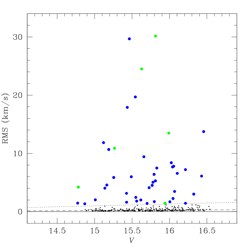
Figure 7: Radial velocity RMS for all stars in our catalog as a function of magnitude. The dashed line denotes the magnitude dependent RMS treshold described in the text, the dotted line denotes the 5$\rm\sigma$ detection treshold. Blue points are RMS variables and green points are GLS variables.

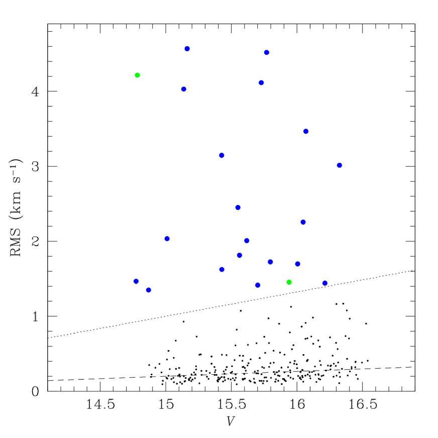
Figure 8: Radial velocity RMS for all stars in our catalog in the region below 5 km $\rm\,s^{-1}$.

Figure 7 shows the RMS distribution for all the catalog stars. We adopted a magnitude dependent treshold for the detection of variables as visible in Fig. 8. This RMS treshold ($\rm\sigma_{ref}$) was calculated by medianing the RMS values of the stars found in 0.2 mag bins and fitting a linear model to the resulting median values. We adopted a 5$\rm\sigma_{ref}$ treshold denoted by the dotted line in the above mentioned Figures. All objects beyond this treshold were considered bona-fide variables and are denoted in particular by the blue dots.

We also searched for periodic variables given the extent of our survey and the fact that many objects have multiple measurements in our catalog. In particular we limited the search for periodicities to stars with at least 10 epochs. We used the Generalized Lomb Scargle (GLS) algorithm of Zechmeister & Kūrster (2009) and in particular their Eq. 5. This algorithm allows to fit a sinusoid to the data together with a constant offset. To properly set the detection treshold of the GLS we constructed a mock sample of constant artificial radial velocities. The measurements for each star were simulated assuming a gaussian noise with a dispersion equal to $\rm\sigma_{ref}$. We considered the true distribution of epochs of our stars, each simulated star being a constant mock copy of a real observed one. We created around 10⁵ simulated stars and applied the GLS to all of them. We searched for periodic signals considering periods in between 0.5 and 1000 days subdividing this interval in 10000 equal frequency steps. From the distribution of GLS powers ($\rm p_{GLS}$) we obtained, we imposed a False Alarm Probability (FAP) treshold equal to 0.1$\%$, which was found equal to $\rm p_{GLS,FAP}=0.956$.

In the exactly same way we applied the GLS to all real measurements flagging out all objects having $\rm p_{GLS}\,>\,p_{GLS,FAP}$. We found that this condition was met for 28 objects. We considered however as reliable GLS variables only those for which an orbital solution could be found as described in Sect. 6. Most of the GLS solutions implied long term trends or in any case the phase coverage was not considered sufficient to perform a fit. All of these objects lie beyond the 5$\rm\sigma_{ref}$ treshold and are therefore also RMS variables.

The final list of reliable GLS variables contains 6 objects which are denoted by the green dots in Figure 7 and Figure 8. The total list of variables contains 45 stars.

5 Classification of the stars

We proceeded by calculating the average radial velocity of the cluster. To do that we used both the proper motion probabilities derived in M09 and the radial velocities calculated in this work. We first considered those objects for which the proper motion membership probability was larger than 90$\%$ at magnitude $V=$12.5 and larger than 50$\%$ at $V=18$, interpolating linearly between these extremes. Furthermore, we impose that the corresponding x and y coordinates of these stars should have been contained within $800<x<1300$, $1000<y<3000$ in the reference system of CCD51 of the Wide Field Imager detector where the cluster was located in M09. Beyond these limits we considered our proper motions doubtful as reported in earlier works. These tresholds are the same adopted in the past to isolate cluster members. We also limited the sample to stars that were not flagged out as variables accordingly to the analysis performed in the previous Section. In this way we identify 66 stars. The average cluster radial velocity $\rm\overline{RV}_{cl}$ we obtained is

$$\rm\overline{RV}_{cl}=(-28.81\pm 0.003)\,km\,\rm s^{-1}$$ (2)

where the error quoted is the error of the mean. The RMS was $\rm\sigma_{cl}$=1.05 km $\rm s^{-1}$. To obtain this result we used 1531 individual measurements.

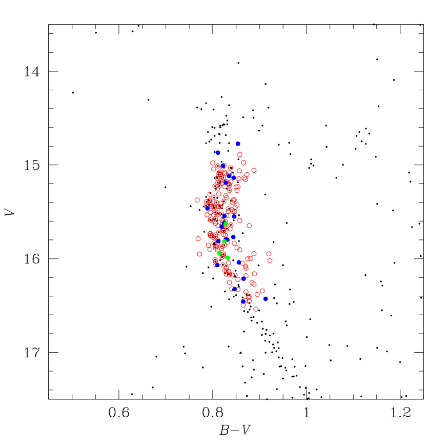
Figure 9: Color magnitude diagram for cluster members. Blue and green dots represent RMS and GLS variables respectively. Red open circles represent radial velocity constant stars. On the background the CMD of proper motion members from the M09 catalog.

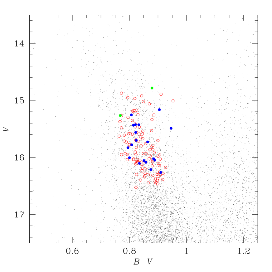
Figure 10: The same as Fig.9 for field stars.

We proceeded as follows to classify all our stars into likely cluster members and likely field stars. Cluster members were identified as stars which proper motion probability was satisfying the constraints reported above and which average radial velocity was in between $\pm$3$\rm\sigma_{cl}$ from the cluster mean average velocity . In absence of proper motions (or in the case proper motions were considered doubtful) we considered as bona fide members those stars satisfying only the radial velocity criterium. The total sample of cluster stars is equal to 192 stars, 25 of which were flagged out as variables. Consequently, the sample of field stars contains 121 stars, 20 of which are variables. On the basis of this classification we obtain an observed frequency of variables equal to 13$\%$ for the cluster, and equal to 17$\%$ for the field. We also obtain that the overall field contamination is around 38$\%$. Some caveats should be kept in mind however. Among all cluster members only 59 satisfy the stringent constraints on proper motions and radial velocity, the remaining ones are only radial velocity members. Therefore a certain field contamination can be expected from field stars sharing the same velocity of cluster members. Equivalently, among field variables some fail to satisfy the radial velocity criterium but have high proper motion probabilities. Since they are variables, their average radial velocity is not necessarily coincident with the systemic velocity. Figure 9 and Figure 10 show the color magnitude diagrams for cluster and field stars respectively. In the background we displayed also proper motion likely members from our catalog in the first case and all other objects in the second. From these figures it is clear that field stars are much more dispersed in the CMD, and that cluster members closely follow the main sequence of the cluster. Blue and green dots have the same meaning than previous figures, denoting respectively RMS and GLS variables. Red open dots denote constant stars.

Table 2 and Table 3 show the complete list of variables along with their basic parameters.

6 Analysis of periodic variables

For six variables we were able to derive an orbital solution. The period was fixed to the GLS period corresponding to the peak with the strongest power. We modeled the Keplerian motion as:

$$\rm RV\,=\,\tilde{K}\frac{\cos u+k}{\sqrt{1-h^{2}-k^{2}}}+\gamma$$ (3)

where $\tilde{K}$ is the radial velocity semi-amplitude without the contribution of the eccentricity $e$, $k=e\,\cos\omega$, $h=e\,\sin\omega$, $\gamma$ is the barycentric radial velocity and $u=\nu+\omega$ is the true argument of latitude with $\nu$ the true anomaly and $\omega$ the argument of the pericenter.

We considered as free parameters: $\tilde{K}$, $h$, $k$, the time of maximum radial velocity ($t_{MAX}$) and $\gamma$. The convergence toward the best-fit solution was obtained by means of a Levenberg-Marquardt algorithm (Press 1992), and the uncertainties and the best fit values of the parameters by means of a Markov Chain Monte Carlo analysis. For each radial velocity curve we created 20 chains of 10⁵ steps. Each chain is started from a point 5-$\sigma$ away (in one randomly selected free parameter) from the best-fitting solution obtained by the Levenberg-Marquardt algorithm. The $\chi^{2}_{\rm old}$ of the fit of this initial solution is recorded and compared with the $\chi^{2}_{\rm new}$ obtained in the following step. The following step is obtained jumping from the initial position to another one in the multidimensional parameter space randomly selecting one of the free parameters and changing its value by an arbitrary amount which is dependent on a jump constant and the uncertainty $\sigma$ of the parameter itself. Steps are accepted or rejected accordingly to the Metropolis-Hastings criterium. If $\chi^{2}_{\rm new}$ is lower than $\chi^{2}_{\rm old}$ the step is executed, otherwise the execution probability is $P=e^{-\Delta\chi^{2}/2}$ where $\Delta\chi^{2}=\chi^{2}_{\rm new}-\chi^{2}_{\rm old}$. In this latter situation a random number between 0 and 1 is drawn from a uniform probability distribution. If this number is lower than $P$ then the step is executed, otherwise the step is rejected and the previous step is repeated instead in the chain. In any case the value of the $\chi^{2}$ of the last step is recorded and compared with the one of the following step up to the end of the chain. We adjusted the jump constants (one for each parameter) in such a way that the step acceptance rate for all the parameters was around 25 per cent. We then excluded the first 20 per cent steps of each chain to avoid the initial burn-in phase, and for each parameter we merged the remaining part of the chains together. Then we derived the mode of the resulting distributions, and the 68.3 per cent confidence limits defined by the 15.85th and the 84.15th percentiles in the cumulative distributions.

The radial velocity measurements after subtraction of the barycentric velocities, along with the best fit model, bisector diagram and the periodogram are shown in Fig. 12-Fig. LABEL:fig:v478. Our best-fit parameters are given in Table 4. The best-fit models correspond to values of the reduced $\chi$ squared between $\sqrt{\chi_{r}^{2}}=0.8-2.5$.

The bisector error was calculated from the dispersion of the distribution of bisector values of all the spectra, and assumed identical for all stars. We also checked for linear correlations between the bisector and radial velocity measurements calculating the Pearson correlation coefficient. For the six cases considered the coefficient is comprised in between -0.47 and 0.56 which denoted that no strong correlations are found.

For those variables that were considered cluster members (4 out of 6 as shown in Table 4) we also calculated the mass function and, by assuming for the primary the mass ($\rm M_{*}$) obtained by isochrone fit we report in Table 4 a lower limit on the minimum mass of the companion which is given by the following equation

$$\rm m\,sin\,i>\Big{(}M^{2}_{*}\frac{\tilde{K}^{3}\,P}{2\,\pi\,G}\Big{)}^{\frac{1}{3}}$$ (4)

the value given by the expression on the right represents a lower limit on the minimum mass because we neglected the term on the mass ratio $\rm q=m/M_{*}$, which contributes as $\rm(1+q)^{2/3}$ to the numerator of the term on the right. The values we obtained are in between $\sim$90 $\rm M_{J}$ and $\sim$460 $\rm M_{J}$. The periods instead are in between $\sim$3 days and $\sim$220 days. We note that the attribution of the exact period is still ambiguous for some objects. Among this sample of objects star 478 seems to have a non negligible eccentricity e=(0.16$\pm$0.03). For star 29531 instead the $\chi_{r}$ of the fit is 2.5 and this may suggest the presence of an additional companion.

7 Comparison with previous surveys

So far four main surveys have been performed toward NGC 6253 to search for variables. As reported in the introduciton De Marchi et al. (2010) and Kaluzny et al. (2014) searched for photometric variables. Anthony-Twarog et al. (2010) and M11 searched for radial velocity variables.

We observed the detached eclipsing binary V23 (39883 in our catalog) reported in Kaluzny et al. (2014). This object is a proper motion member of NGC 6253 and sits close to the turn-off. We obtained only 1 measurement on it which gave a radial velocity equal to (-52.96$\pm$0.18) km$\rm\,s^{-1}$.

The star 16649 was classified in De Marchi et al. (2010) as a long period variable, likely cluster member and located at around 7 arcmin from the cluster center. It showed a photometric variability at the 1$\%$ level. This object has been extensively observed here. A set of 32 measurements have been acquired. It results that star 16649 is also a radial velocity variable and it is listed in Table 2 as a likely cluster member variable. The mean radial velocity is -28.446 km$\rm\,s^{-1}$ and the RMS is 7.7 km$\rm\,s^{-1}$. Membership is estabilished solely on the basis of radial velocity. The GLS algorithm flagged out this star as a variable, but at the nominal period ($\sim$63 days) it presents a very poor phase coverage and no orbital solution was possible. These observations support the idea that this object is a long period binary system. It is curious to note that in fact, this object was also observed by Anthony-Twarog et al. (2010) during the Hydra radial velocity survey on NGC6253. Also in that case star 16649 (corresponding to star 7592 in their numeration) was found a radial velocity variable star. The authors report a mean radial velocity equal to -27.38 km$\rm\,s^{-1}$ and an RMS equal to 10 km$\rm\,s^{-1}$ measured out of a set of 3 measurements.

The interesting star 55053 was also listed in De Marchi et al. (2010) as a long period variable, likely cluster member. It is located at around 5.2 arcmin from the cluster center. In our study we obtained a set of 15 radial velocity measurements on it. Interestingly, this object is not a radial velocity variable, at least down to 0.4 km$\,\rm\,s^{-1}$, the value we calculated for the RMS. In our study it is classified as a radial velocity non variable cluster member. Membership is estabilished on the basis of radial velocity given that the average velocity is -28.613 km$\rm\,s^{-1}$.

No matches were found with our previous radial velocity survey presented in Montalto et al. (2011), because there we focused on brighter objects.

The overlap with the Anthony-Twarog et al. (2010) survey is instead substantial. We counted a total of 32 stars in common among the two surveys which gives us the opportunity to further check for long-term variability for these objects. Comparing our radial velocities with the ones of the authors we found in general an excellent agreement.

Star 21659 is an interesting variable that was discovered by Anthony-Twarog et al. (2010). The authors report an RMS equal to 19.5 km$\,s^{-1}$ for this object (their star 7495) and cosidered it among their list of five likely cluster variable stars. In our study this object was classified as well as a cluster variable. In addition to that it is among the list of objects for which we derived the orbital solution, as reported in Table 4. The radial velocity semi-amplitude we found (41.8 km$\rm\,s^{-1}$) is consistent with the RMS reported by Anthony-Twarog et al. (2010).

Star 8247 (7303 in Anthony-Twarog et al. 2010) was considered as a likely member cluster variable by the authors which gave an RMS equal to 16.4 km$\rm\,s^{-1}$. In our data this object is instead not variable, but we note that our mean radial velocity differs from the one of the authors by 13 km$\rm\,s^{-1}$. This object is likely a long period cluster variable.

On the contrary star 7470 in Anthony-Twarog et al. (2010, which does not have an entry in our own catalog), is in the list of our likely cluster variables in Table 2, having an RMS equal to 4.519 km$\rm\,s^{-1}$. Anthony-Twarog et al. (2010) did not consider this object as a variable, but their RMS is similar to us (3.24 km$\rm\,s^{-1}$), quite larger than their average level, although probably at the limit of detectability.

8 Discussion

The survey we presented in this work is one of the deepest searches for binaries in an old open cluster ever performed so far. Milliman et al. (2014), based on their on going long-term radial velocity monitoring of the old open cluster NGC 6819 concluded that the fraction of binaries with periods less than 10⁴ days is equal to 22$\,\%\,\pm\,$3$\%$. Our total frequency is lower as reported below, but it is also based on a 2 year survey while Milliman et al. (2014) are monitoring NGC 6819 since 17 years. Binaries surveys in the field (albeit including a variety of detection methods) suggest that the total multiplicity fraction around field stars is around 54$\%$ (e. g. Raghavan et al. 2010).

To understand our detection limits and binary fractions we performed a set of simulations. Similarly to what was done in Sect. 4, we created a mock sample of measurements for each observed star, assuming the baseline noise level $\rm\sigma_{ref}$ and injecting an artificial signal into the data to mimick the presence of a companion star. We randomized both the phase and the inclination of the orbits and considered 25 bins in true mass (between 20 and 500 $\rm M_{J}$) and an orbital period equal either to 10 days or to 200 days. We therefore applied the 5$\rm\sigma_{ref}$ treshold calculating the detection efficiency in each mass bin. Figure 11, shows the detection efficiency curves for the two periods considered as a function of the companion mass. Those curves are essentially average efficiencies over the whole sample of stars monitored. The simulations indicate that at a period of 10 days, objects with masses down to $\sim$30 M_J could have been detected with a $\sim$50$\%$ efficiency. At 90$\%$ confidence limit we expect to be able to detect stars with at least 0.15 M_⊙. Considering a period of 200 days, a 50$\%$ detection efficiency corresponds to $\sim$0.1 M_⊙, and a 90$\%$ detection efficiency to $\sim$0.4 M_⊙.

Looking at the results we obtained in Tab. 4, we conclude that essentially for all the detected objects, the detection efficiency should be beyond 80$\%$. The only exception is star 30324 which has a long period (223 days) and a low minimum mass (92 M_J) and may indeed lie in a $\sim 50\%$ efficiency region. If the true mass of this object is close to the limit indicated by its minimum mass, this would indicate that a correcting factor at least equal to 2 should be applied to derive the true frequency of stars with long period companions. This may also be supported by the fact that for most of the variable objects we detected it was not possible to derive an orbital solution.

Considering therefore only the sample of close-in cluster members variables for which an orbital solution was found, we conclude that the frequency of binaries down to the hydrogen burning limit and with periods up to $\sim$20 days is around (1.5$\pm$1.3)$\%$, that is 3 out 200 members, in the upper main sequence of NGC 6253, while the total binary frequency is equal to (13$\pm$3)$\%$. The errors were obtained considering a binomial distribution.

Comparatively, in M11 we obtained a frequency of binaries equal to (29$\pm$9)$\%$. These binaries were all flagged out with a 5$\rm\sigma$ detection treshold like in this work and were considered likely short period binaries given that the observations spanned only a few days. The sample of cluster stars (35) was much smaller than the one analyzed in this work which gives a larger uncertainty for the estimated frequency. Even accounting for that, it appears however that the frequency among evolved stars is larger (at a 2-$\sigma$ level) than the total frequency of binaries on the main sequence we obtained above.

9 Conclusions

We described an extensive radial velocity survey toward the old and metal rich open cluster NGC 6253. The survey was performed during two seasons between April 2004 and July 2005 using the FLAMES spectrograph monitoring a total number of 317 stars with a median number of 15 epochs per star. A more limited follow up of 7 objects was performed with the HARPS spectrograph in June 2011.

We obtained a median precision equal to 240 m$\rm\,s^{-1}$ for the GIRAFFE spectrograph, 180 m$\rm\,s^{-1}$ for UVES and 35 m$\rm\,s^{-1}$ for HARPS, working in a magnitude range in between 14.8$<V<$16.5. Among the sample of monitored stars, 59 are now classified as radial velocity and proper motion cluster members and do not show any evidence of variability. Field contaminations was equal to 38$\%$ of the total sample.

In total we found 45 variable stars, among which 25 are considered cluster members and 20 field objects. For 6 spectroscopic binaries we obtained the orbital solution, which implied minimum masses in between $\sim$90 M_J-$\sim$460 M_J and orbital periods in between $\sim$3 days and $\sim$220 days.

The frequency of binaries down to the hydrogen burning limit and up to 20 days orbital period is found equal to (1.5$\pm$1.3)$\%$. in the upper main sequence of NGC 6253, while the total binary frequency is equal to (13$\pm$3)$\%$.

The precisions achieved by the HARPS spectrograph are sufficient to further extend the exploration of the binary frequency well within the substellar domain, and to analyze the high mass end of the planetary domain (down to 4-5 M_J). The upcoming ESPRESSO spectrograph at VLT will represent an even more powerful tool to study planetary frequencies in stellar clusters. A precision of around 5 m$\rm\,s^{-1}$ may be expected with similar exposure times on our targets. This will push further our exploration well within the planetary domain, down to around half a jupiter mass.

Table 1: Observations

Observing time	Exposure time	Instrument	Dates
58hr	900s-3600s	UVES/GIRAFFE	2/4/2004-15/7/2004
38.5hr	2020s-2700s	UVES/GIRAFFE	3/5/2005-1/7/2005
13.5hr	680s-3600s	HARPS	28-30/05/2011

Table 2: Cluster variables^a

ID	RA(J2000)	DEC(J2000)	B-V	V	N. obs.	$\rm\overline{RV}$ (km $\rm s^{-1}$)	RMS(km $\rm s^{-1}$)	P($\%$)b
39667	254.732063568	-52.736025614	0.845	15.137	42	-29.087	4.030	88.
29531	254.699632781	-52.704366462	0.828	15.628	28	-27.300	24.509	89.
33955	254.700423295	-52.630001667	0.832	15.990	26	-29.945	13.486	90.
31617	254.689311198	-52.669417089	0.831	15.797	11	-28.108	1.725	91.
39854	254.781010467	-52.723246777	0.828	15.189	3	-30.762	10.677	94.
43081	254.767887749	-52.693853688	0.835	15.119	17	-30.744	11.849	93.
31834	254.734726224	-52.665662838	0.810	16.068	25	-26.430	3.467	82.
30324	254.746004485	-52.690480237	0.814	15.940	41	-28.595	1.455	$-$
21659	254.876860986	-52.797707300	0.825	15.814	37	-29.166	30.154	$-$
39831	254.854747288	-52.724276741	0.789	15.464	36	-26.177	29.672	93.
$-$	254.871791667	-52.737444444	0.822	15.010	19	-29.012	2.035	$-$
35905	254.658158455	-52.596792279	0.866	16.213	6	-28.896	7.217	24.
$-$	254.979041667	-52.729833333	0.844	15.769	7	-28.434	4.519	$-$
24648	254.756000212	-52.791118012	0.913	16.428	39	-26.037	6.109	0.
49148	254.607856534	-52.777415622	0.846	15.550	7	-25.939	2.451	$-$
34667	254.708667366	-52.617760801	0.865	16.456	31	-29.062	13.748	85.
16649	254.892499238	-52.618200382	0.856	16.040	32	-28.446	7.678	$-$
30290	254.850999373	-52.690813347	0.825	15.544	41	-26.183	19.692	90.
$-$	254.794625000	-52.807416667	0.847	16.324	39	-29.067	3.014	$-$
14466	254.902801435	-52.714731958	0.854	14.774	28	-26.381	1.467	$-$
27965	254.847398993	-52.732799296	0.812	15.812	19	-28.740	5.294	70.
27341	254.863111261	-52.743533585	0.819	15.658	16	-26.352	9.431	85.
49667	254.600056580	-52.710400816	0.828	15.794	6	-30.035	6.405	$-$
41026	254.645602194	-52.641141858	0.811	14.869	22	-31.695	1.350	6.
$-$	254.977791667	-52.770055556	0.825	15.617	6	-28.714	2.009	$-$

a –   Below the horizontal line membership is estabilished only on the basis of radial velocities.
b –   Proper motion membership probability.

Table 3: Field variables

ID	RA(J2000)	DEC(J2000)	B-V	V	N. obs.	$\rm\overline{RV}$ (km $\rm s^{-1}$)	RMS(km $\rm s^{-1}$)	P($\%$)
31505	254.687118376	-52.671306636	0.864	15.728	41	-25.258	4.116	91.
478	254.923022901	-52.809584139	0.879	14.783	35	-55.207	4.216	$-$
40696	254.778223506	-52.662991026	0.807	15.255	23	-24.845	5.866	95.
28889	254.782822852	-52.715868624	0.824	15.701	29	-24.585	1.415	90.
27108	254.786303150	-52.747918476	0.821	15.426	41	-23.120	3.147	89.
28017	254.789168050	-52.731954093	0.814	15.436	25	-36.817	17.897	92.
9156	254.897722920	-52.620682013	0.875	16.213	6	-2.398	1.442	$-$
$-$	254.956791667	-52.780388889	0.851	16.056	25	-24.514	7.795	$-$
39659	254.842084425	-52.736277043	0.768	15.266	30	-28.756	10.886	28.
49446	254.621343512	-52.739416289	0.905	15.163	40	-12.317	4.569	$-$
9756	254.913463429	-52.608067153	0.910	16.263	8	-71.134	66.779	$-$
28733	254.790227260	-52.718374337	0.795	15.830	27	-26.188	7.492	56.
23507	254.713571036	-52.811072103	0.808	15.779	36	-25.407	5.046	$-$
31512	254.810969168	-52.670869985	0.822	15.562	36	-32.037	1.814	90.
$-$	254.933625000	-52.587555556	0.889	16.047	2	-21.799	2.256	$-$
10638	254.903502113	-52.587731891	0.946	15.490	8	-11.044	5.990	$-$
$-$	254.865708333	-52.674027778	0.885	16.024	37	-61.851	8.402	$-$
23848	254.736362325	-52.805171881	0.835	16.104	14	-100.238	6.578	$-$
24548	254.742155375	-52.792685121	0.800	16.005	23	-93.670	1.698	0.
$-$	254.769458333	-52.707944444	0.833	15.427	5	-23.596	1.624	$-$

Table 4: Spectroscopic binaries

ID	Period (days)	$\rm\tilde{K}$(m $\rm s^{-1}$)	e cos$\rm\,\omega$	e sin$\rm\,\omega$	$\rm t_{MAX}$ (HJD-2450000)	$\gamma$(km $\rm s^{-1}$)	P($\%$)	m sin i ($\rm M_{J}$)	$\chi_{red}$
29531	3.204288	35800${}_{-79}^{+79}$	-0.0018${}_{-0.0033}^{+0.0033}$	-0.00788${}_{-0.0027}^{+0.0019}$	3201.39496${}_{-0.0028}^{+0.0013}$	-27.30048${}_{-0.047}^{+0.075}$	89	279	2.5
30324	224.118409	3000${}_{-146}^{+134}$	-0.091${}_{-0.051}^{+0.021}$	-0.12344${}_{-0.0277}^{+0.0099}$	3561.65496${}_{-0.71}^{+0.83}$	-28.59548${}_{-0.074}^{+0.062}$	$-$	92	0.8
21659	9.967883	41800${}_{-70}^{+65}$	-0.0047${}_{-0.0012}^{+0.0010}$	0.00345${}_{-0.0025}^{+0.0015}$	3522.36771${}_{-0.0024}^{+0.0017}$	-29.16622${}_{-0.052}^{+0.027}$	$-$	466	1.3
33955	8.808062	21000${}_{-65}^{+147}$	-0.0015${}_{-0.0036}^{+0.0054}$	-0.00248${}_{-0.0039}^{+0.0033}$	3552.49403${}_{-0.0035}^{+0.0047}$	-29.94483${}_{-0.085}^{+0.043}$	90	220	1.0
39659a	7.651044	13500${}_{-119}^{+171}$	0.0027${}_{-0.017}^{+0.0061}$	0.02813${}_{-0.0113}^{+0.0049}$	3144.08394${}_{-0.018}^{+0.013}$	-28.75597${}_{-0.098}^{+0.058}$	28	146	1.2
478a	23.846401	6100${}_{-60}^{+81}$	-0.1612${}_{-0.0093}^{+0.010}$	-0.03923${}_{-0.0080}^{+0.0094}$	3149.34776${}_{-0.077}^{+0.021}$	-55.20715${}_{-0.053}^{+0.053}$	$-$	102	1.5

a –   Field star

Figure 1: Observed S/N for the spectra acquired with each GIRAFFE setting used in this work and with the UVES spectrograph (bottom right panel).

Figure 2: Plate to plate radial velocity systematics for GIRAFFE and UVES as a function of plate number (top panels). In the bottom panel we report the histogram of the difference between the average radial velocity calculated in the GIRAFFE reference system (<RV_G>) and in the UVES reference system (<RV_U> and <RV_L> for the upper and lower UVES spectra respectively). Only GIRAFFE reference stars having also 5 UVES radial velocity measurements (34 stars) are considered.

Figure 3: Average subtracted radial velocities for GIRAFFE and UVES spectrographs during different stages of post-processing as reported in the panels and in the text. The continuous line represents the best-fit Gaussian to the residual distributions.

Figure 4: Radial velocity residuals for each GIRAFFE setting.

Figure 5: Top: histogram of radial velocity corrected RMS for all stars with at least two measurements and RMS below 1 km s^-1 observed with GIRAFFE (top), UVES (middle) and in the combined catalog (bottom). The dashed vertical lines denote median values.

Figure 6: Histogram of all radial velocities measurements acquired with the FLAMES spectrograph.

Figure 11: Survey detection tresholds as a function of the companion mass and period.

Figure 12: Folded RV curve with best fit model and residuals (top), bisector (middel) and periodogram (bottom) for star 21659. The dashed horizontal line in the periodogram panel denotes the GLS algorithm detection treshold (p_GLS,FAP) as defined in the text.

Figure 13: Folded RV curve with best fit model and residuals (top), bisector (middel) and periodogram (bottom) for star 29531. The dashed horizontal line in the periodogram panel denotes the GLS algorithm detection treshold (p_GLS,FAP) as defined in the text.

Figure 14: Folded RV curve with best fit model and residuals (top), bisector (middel) and periodogram (bottom) for star 30324. The dashed horizontal line in the periodogram panel denotes the GLS algorithm detection treshold (p_GLS,FAP) as defined in the text.

Figure 15: Folded RV curve with best fit model and residuals (top), bisector (middel) and periodogram (bottom) for star 33955. The dashed horizontal line in the periodogram panel denotes the GLS algorithm detection treshold (p_GLS,FAP) as defined in the text.

Figure 16: Folded RV curve with best fit model and residuals (top), bisector (middel) and periodogram (bottom) for star 39659. The dashed horizontal line in the periodogram panel denotes the GLS algorithm detection treshold (p_GLS,FAP) as defined in the text.

References

- [2007] Anthony-Twarog, B. J., Twarog, B. A. & Mayer L. 2007, AJ, 133, 1585
- [2010] Anthony-Twarog, B. J., Deliyannis, C. P., Twarog, B. A., Cummings, J. D., Maderak, R. M. 2010, AJ, 139, 2034
- [1997] Bragaglia, A., Tessicini, G., Tosi, M., Marconi, G., Munari, U. 1997, MNRAS, 284, 477
- [2000] Carretta, E., Bragaglia, A., Tosi, M., Marconi, G. 2000, ASPC, 198, 273
- [2007] Carretta, E., Bragaglia, A. & Gratton, R. G. 2007, A&A, 473, 129
- [2012] Cummings, J. D., Deliyannis, C. P., Anthony-Twarog, B., Twarog, B., Maderak, R. M. 2012, AJ, 144, 137
- [2010] De Marchi, F., Poretti, E., Montalto, M., Desidera, S., Piotto, G. 2010, A&A, 509, 17
- [2005] Fischer, D. A. & Valenti, J. 2005, ApJ, 622, 1102
- [2013] Freudling, W., Romaniello, M., Bramich, D. M., Ballester, P., Forchi, V., García-Dabló, C. E., Moehler, S., Neeser, M. J. 2013, A&A, 559, 96
- [1997] Gonzalez, G. 1997, MNRAS, 285, 403
- [2014] Kaluzny, J., Rozyczka, M., Pych, W., Thompson, I. B. 2014, AcA, 64, 77
- [2003] Mayor, M., Pepe, F., Queloz, D., Bouchy, F., Rupprecht, G., Lo Curto, G., Avila, G., Benz, W. et al. 2003, The Messenger, 114, 20.
- [2015] Malavolta, L., Piotto, G., Bedin, L. R., Sneden, C., Nascimbeni, V., Sommariva, V. 2015, MNRAS, 454, 2621
- [2012] Mikolaitis, S̆., Tautvais̆ienė, G., Gratton R., Bragaglia, A., Carretta, E. 2012, A&A, 541, 137
- [2014] Milliman, K. E., Mathieu, R. D., Geller, A. M., Gosnell, N. M., Meibom, S., Platais, I. 2014, AJ, 148, 38
- [2009] Montalto, M., Piotto G., Desidera, S., Platais, I., Carraro, G., Momany, Y., De Marchi, F., Recio-Blanco, A. 2009, A&A, 505, 1129, (M09)
- [2011] Montalto, M., Villanova, S., Koppenhoefer, J., Piotto, G., Desidera, S., De Marchi, F., Poretti, E., Bedin, L. R. et al. 2011, A&A, 535, 39, (M11)
- [2012] Montalto, M., Santos, N. C., Villanova, S., Pace, G., Piotto, G., Desidera, S., De Marchi, F., Pasquini, L. et al. 2012, MNRAS, 423, 3039
- [2012] Mortier, A., Santos, N. C., Sozzetti, A., Mayor, M. Latham, D., Bonfils, X., Udry, S. 2012, A&A, 543, 45
- [2002] Pasquini, L., Avila, G., Blecha, A., Cacciari, C., Cayatte, V., Colless, M., Damiani, F., De Propris, R. et al. 2002, The Messenger, 110, 1.
- [1998] Piatti, A. E., Clariá, J. J., Bica, E., Geisler, D., Minniti, D., 1998, AJ, 116, 801
- [1992] Press W. H., Teukolsky S. A., Vetterling W. T., Flannery B. P. 1992, Cambridge: University Press, c1992, 2nd ed.
- [2001] Queloz, D., Henry, G. W., Sivan, J. P., Baliunas, S. L., Beuzit, J. L., Donahue, R. A., Mayor, M., Naef, D. et al. 2001, A&A 379, 279
- [2010] Raghavan, D., McAlister, H. A., Henry, T. J., Latham, D. W., Marcy, G. W., Mason, B. D., Gies, D. R., White, R. J. 2010, ApJS, 190, 1
- [2014] Rozyczka, M., Kaluzny, J., Thompson, I. B., Dotter, A., Pych, W., Narloch, W. 2014, AcA, 64, 233
- [2001] Sagar, R., Munari, U., & de Boer, K. S. 2001, MNRAS, 327, 23
- [2001] Santos, N. C., Israelian, G., Mayor, M. 2001, A&A, 373, 1019
- [2004] Santos, N. C., Israelian, G. & Mayor, M. 2004, A&A, 415, 1153
- [2007] Sestito, P., Randich, S. & Bragaglia, A. 2007, A&A, 465, 185
- [2008] Stoehr, F., White, R., Smith, M., Kamp, I., Thompson, R., Durand, D., Freudling, W., Fraquelli, D. et al. 2008, ASPC, 394, 505
- [2003] Twarog, B. A., Anthony-Twarog, B. J., & De Lee, N. 2003, AJ, 125, 1383
- [2003] Zechmeister, M. & Kūrster, M. 2009, A&A, 496, 577