On parallel solution of ordinary differential equations

Abstract

In this paper the performance of a parallel iterated Runge-Kutta method is compared versus those of the serial fouth order Runge-Kutta and Dormand-Prince methods. It was found that, typically, the runtime for the parallel method is comparable to that of the serial versions, thought it uses considerably more computational resources. A new algorithm is proposed where full parallelization is used to estimate the best stepsize for integration. It is shown that this new method outperforms the other, notably, in the integration of very large systems.

1 Introduction

The numerical solution of an initial value problem given as a system of ordinary differential equations (ODEs) is often required in engineering and applied sciences, and is less common, but not unusual in pure sciences. For precisely estimating asymptotic properties of the solutions, the global truncation errors must be kept lower than the desired tolerance during a very large number of iterations. This is usually achieved by using an adaptive algorithm for the estimation of the largest step for integration yielding a local truncation error below the tolerance. Nevertheless, such a correction usually leads to a drastic increase of the computational time. On the other hand, the use of spectral methods to solve parabolic and hyperbolic partial differential equations (PDE) is becoming more and more popular. The spectral methods reduce these PDEs to a set of ODEs [1]. The higher the desired precision for the numerical solution, the larger the resulting system of ODEs. Very large systems arise also in simulations of multi–agent systems [2]. It can take hours to integrate this kind of systems over a few steps. Taking all the above into account, it can be concluded that devising improved algorithms to compute the numerical solution of ODE systems is still a very important task.

With the steady development of cheap multi-processors technology, it is reasonable to consider using parallel computing for speeding up real-time computations. Particularly interesting are the current options for small-scale parallelism with a dozen or so relatively powerful processors. Several methods have been deviced with that aim (see for instance Refs. [3, 4, 5]), many warranting a substantial reduction of the runtime. For instance, the authors in Ref.[4] claim that the performance of their parallel method is comparable to that of the serial method developed by Dormand and Prince [6] and, in terms of the required number of evaluations of the right–hand side of the ODEs, demonstrates a superior behaviour.

The aim of this work was twofold. Firstly, we wished to test these claims by solving ODEs systems with different degree of complexity over different ranges of time; secondly, we proposed and tested a new method which focuses on taking full advantage of parallel computing for estimating the optimal stepsize. All our codes were written in C and for parallalel programing we used the OPENMP resources. The programs were tested in a server Supermicro A+ 1022GG-TF with 24 CPUs and 32 gigabytes of operational memory.

In the next section, we describe the numerical methods we used for our tests, the standard fourth order Runge-Kutta, a version of the Dormand-Prince method and the parallel iterated Runge-Kutta method proposed in Ref.[4]. These last two methods are widely regarded to be amongst the best options for serial and parallel numerical solution of ODEs. It is also briefly described how the optimal stepsize is estimated in each case. In section 3 the initial value problems used for testing the methods are described. Next, in section 4 we report the results of our comparison of the performance of these methods. In section 5 we introduce an adaptive stepsize parallel algorithm coupled to the Dormand-Prince integrator, and report the results of the corresponding tests. Finally, in section 6 we present our conclusions.

2 Numerical integrators and local error control

Let the initial value problem be specified as follows,

$$\dot{y}=f(t,y)\,,\quad y(t_{0})=y_{0}\,.$$ (1)

Here $y(t)$ is the vector solution at time $t$, dot stands for the derivative with respect to time and the right–hand side of the equation defines a vector field.

Our aim is to compare the performance of several methods for approximating the solution of this problem. All of them are members of the family of explicit Runge–Kutta methods and aproximate $y(t)$ at $t_{n+1}=t_{n}+h$ as

$$y_{n+1}=y_{n}+h\displaystyle\sum\limits_{i=1}^{s}b_{i}k_{i}\,,$$ (2)

where

$$k_{1} = f(t_{n},y_{n})\,,$$

$$k_{2} = f(t_{n}+c_{2}h,y_{n}+ha_{21}k_{1})\,,$$

$$k_{3} = f(t_{n}+c_{3}h,y_{n}+h(a_{31}k_{1}+a_{32}k_{2})\,,$$

$$\vdots$$

$$k_{s} = f(t_{n}+c_{s}h,y_{n}+h(a_{s1}k_{1}+a_{s2}k_{2}+\cdots a_{s,s-1}k_{s-1})\,,$$ (3)

and $s$ is known as the number of stages. Therefore, a method with $s$ stages usually requires, at least, $s$ evaluations of the right–hand side of the system at each iteration.

A Runge–Kutta method can be especified by a Butcher tableau like in table 1.

$$\begin{array}[]{ c | c c c c c }0\\ c_{{}_{2}}&a_{{}_{21}}\\ c_{{}_{3}}&a_{{}_{31}}&a_{{}_{32}}\\ \vdots&\vdots&\vdots&\ddots\\ c_{{}_{s}}&a_{{}_{s1}}&a_{{}_{s2}}&\ldots&a_{{}_{s,s-1}}\\ \hline\cr\rule{0.0pt}{11.19443pt}&b_{{}_{1}}&b_{{}_{2}}&\ldots&b_{{}_{s-1}}&b_{{}_{s}}\end{array}$$

Table 1: Butcher tableau

The order of a method is $p$ if the local truncation error is on the order of $\mathcal{O}(h^{p+1})$, while the total accumulated error is of order $\mathcal{O}(h^{p})$. The higher the order of the method, the lower the error of the approximation, nevertheless, constructing higher order Runge–Kutta formulas is not an easy task. To avoid increasing $s$ (and, therefore, the number of evaluations of $f$) a common alternative is to develope methods with adaptive stepsize.

For any numerical method, an estimate for the local truncation error while integrating from $t_{n}$ to $t_{n+1}=t_{n}+h$ is given by

$$\epsilon:=\|y_{n+1}-\bar{y}_{n+1}\|\,,$$ (4)

where $\|\cdot\|$ stands for a given norm, and $y_{n+1}$ and $\bar{y}_{n+1}$ are the results of different numerical approximations of $y(t_{n+1})$. The stepsize yielding a local error below the tolerance ($Tol$) is then given by

$$h_{opt}=h\displaystyle\left(\frac{Tol}{\epsilon}\right)^{\frac{1}{p}}\,.$$ (5)

2.1 Fourth order Runge–Kutta method (RK4)

The method given in table 2 is the classical member of the family of Runge–Kutta methods.

0
1/2	1/2
1/2	0	1/2
1	0	0	1
	1/6	2/6	2/6	1/6

Table 2: “The” Runge–Kutta method

We used RK4 without a stepsize control mechanism. Hence, in all our tests we choose the stepsize in such a way that the global error had the same order of those obtained by the methods with adaptive stepsize.

2.2 Dormand-Prince method (DOP853)

In this method [6], the last stage is evaluated at the same point as the first stage of the next step (this is the so-called FSAL property), so that the number of evaluations of $f$ is one less than the number of stages. Here there is no easy way to present the Butcher coefficients in a tableau, because it involves dealing with irrational quantities [5]. The coefficients we use can be found in the code by E. Hairer and G. Wanner available in the site [7].

The approximations $y_{n+1}$ and $\bar{y}_{n+1}$ in equation (4) correspond here to the results obtained using different orders, and the $k_{i}$ are determined by minimizing the error of the higher order result. As a matter of fact, in the version we use two comparisons are made, one between 8th and 5th orders, and the second one between 8th and 3th orders. Then, the error is estimated using [5]:

$$\epsilon=\epsilon_{5}\frac{\epsilon_{5}}{\sqrt{\epsilon_{5}^{2}+0.01\epsilon_{3}}}\,.$$ (6)

2.3 Parallel iterated Runge–Kutta method (PIRK10)

Let us consider a s-stage Runge–Kutta method given by the coefficients

$$A=(a_{ij})_{{}_{i,j=1}}^{{}^{s}},\qquad B^{{}^{T}}=(b_{{}_{1}},\ldots,b_{s}),\qquad C=(c_{{}_{1}},\ldots,c_{s})^{{}^{T}}$$

and let $y_{1}$ be defined as:

$$k_{i}^{{}^{(0)}} =f(x_{{}_{0}},y_{{}_{0}})$$

$$k_{i}^{{}^{(\ell)}} =f(x_{{}_{0}}+c_{i}h,y_{{}_{0}}+h\displaystyle\sum\limits_{j=1}^{s}a_{{ij}}k_{j}^{{}^{(\ell-1)}})\ \ \ \ \ \ell=1,\ldots,m$$ (7)

$$y_{1} =y_{0}+h\displaystyle\sum\limits_{i=1}^{s}b_{i}k_{i}^{{}^{(m)}}$$

Here $m$ is the number of iterations used to estimate $k_{i}$. As it is shown in [4], provided that $s$ processors are available, this scheme represents an explicit Runge–Kutta method. Furthermore, since each $k_{i}^{{}^{(\ell_{{}_{0}})}}$ can be computed in parallel, we have the following theorem,

Theorem 2.1.

Let $\{A,B^{T},C\}$ define an s-stage Runge–Kutta method of order $p_{0}$. Then the method defined by (7) represents an $(m+1)-stage$ explicit Runge–Kutta method of order $p$, where

$$p=\min\{p_{0},m+1\}.$$

One of the advantages of this method is that if we set $m=p_{0}-1$, then the order of the method is equal to the number of stages, which results in less right–hand side evaluations (sequentially). In general the number of stages of explicit Runge–Kutta methods is greater than the order of the method, therefore if an explicit method is used the required number of processors is greater as well.

Along the lines in Ref.[4] and with the Butcher coefficients in table 5 in the Appendix, we implemented a parallel iterated Runge–Kutta method of order $10$. Here, $y_{n}$ and $\bar{y}_{n}$ in equation (4) correspond to the results obtained using different number of iterations for approximating $k_{i}$,

$$y_{{}_{n+1}}=y_{{}_{n}}+h\displaystyle\sum\limits_{i=1}^{s}b_{i}k_{i}^{{}^{(m)}}$$ (8)

and

$$\bar{y}_{{}_{n+1}}=y_{{}_{n}}+h\displaystyle\sum\limits_{i=1}^{s}b_{i}k_{i}^{{}^{(m-1)}}\,.$$ (9)

3 Initial value problems

Next, we list and briefly describe the systems of ODEs that we have used to test the above numerical methods.

3.1 Simple harmonic oscillator (HO)

As a first initial value problem we chose:

$$\begin{cases}\dot{y}_{1}=y_{2}&\qquad y_{1}(0)=0,\\ \dot{y}_{2}=-y_{1}&\qquad y_{2}(0)=1\text{.}\end{cases}$$

Since this system is readily integrable, we used it to assess the quality of the numerical results by comparing with the analytical ones.

3.2 Hénon-Heiles system (HH)

This is a Hamiltonian system which describes the nonlinear dynamics of a star around a galactic center when the motion is constrained to a plane [8]:

$$\begin{cases}\dot{y}_{{}_{1}}&=y_{{}_{2}}\\ \dot{y}_{{}_{2}}&=-y_{{}_{1}}-2y_{1}y_{3}\\ \dot{y}_{{}_{3}}&=y_{{}_{4}}\\ \dot{y}_{{}_{4}}&=-y_{{}_{3}}-y^{2}_{{}_{1}}+y^{2}_{{}_{3}}\end{cases}$$

Since the Hamiltonian $H$ is a constant of motion, it can be used to assess the precision of the numerical solution. We choose initial conditions such that $H=1/6$, yielding a chaotic solution.

3.3 Replicated Hénon-Heiles system (HH100)

To force the integrators to work a little bit harder we constructed a new system by replicating the Hénon-Heiles system $100$ times, resulting in a nonlinear system with $400$ equations:

$$\begin{cases}\dot{y}_{{}_{4i+1}}&=y_{{}_{4i+2}}\\ \dot{y}_{{}_{4i+2}}&=-y_{{}_{4i+1}}-2y_{{}_{4i+1}}y_{{}_{4i+3}}\\ \dot{y}_{{}_{4i+3}}&=y_{{}_{4i+4}}\\ \dot{y}_{{}_{4i+4}}&=-y_{{}_{4i+3}}-y^{2}_{{}_{4i+1}}+y^{2}_{{}_{4i+3}}\,,\end{cases}$$

with $i=0,1,\cdots,99$.

3.4 Gravitational collapse in AdS (GC40) and (GC10)

We also tested the methods by solving the system obtained from the Einstein field equations for the gravitational collapse of a scalar field in anti de Sitter spacetime [9]. Using the Galerkin method [1] the 10 coupled hyperbolic-elliptic nonlinear partial differential equations were converted to a set of $40$ nonlinear ordinary differential equations. The corresponding solutions were shown to be chaotic too [9].

Finally, the last system we used was obtained by reducing the previous one to ten equations .

4 Tests results

To test the methods we ask for the numerical solution of the corresponding problem starting from $t_{0}$ and up to a given $t_{end}$, such that the straigthforward integration with step $h_{0}=t_{end}-t_{0}$ yields a result with an error above the desired tolerance. This implies that, typically, a number of intermediate integrations will be required.

In table 3 is shown the order of the runtime in seconds taken for solving the HO and HH problems in the time interval $0\leq t\leq 2000$ using RK4, DOP853 and PIRK10. In the methods with an adaptive stepsize algorithm we have used a tolerance of $10^{-15}$, what corresponded to using a step $h=0.01$ in the RK4.

$$\begin{array}[]{c|c|c}\rule{0.0pt}{11.19443pt}&HO&HH\\[5.69046pt] \hline\cr DOP853\rule{0.0pt}{11.19443pt}&10^{-2}&10^{-2}\\[5.69046pt] PIRK10&10^{-1}&10^{-1}\\[5.69046pt] RK4&10^{-1}&10^{-1}\\[5.69046pt] \hline\cr\end{array}$$

Table 3: Order of the runtime for the HO and HH problems.

In all the following tests the PRIK10 used its optimal number of 5 processors.

As we can see very similar results were obtained with the three methods, and even though DOP853 seems to be faster, the differences are very small. Nevertheless, the serial methods can be considered to be better than PIRK10 because they are easier to implement and require significantly less computational resources for execution.

Searching for a bigger runtime difference we tested the HH100 problem keeping the same tolerance for DOP853 and PIRK10, but now in the time interval $0\leq t\leq 5000$. This implied to use $h=0.001$ in the RK4. In this case the RK4 and PIRK10 recorded a runtime of $\sim 206$ seconds and $\sim 75$ seconds respectively, both greater than the $\sim 11$ seconds obtained with DOP853.

At this point we recall that, according with theorem 2.1, by using 5 processors the PRIK10 method at each timestep does 9 evaluations of the right-hand-side of the corresponding problem. This is to be contrasted with the, at least, 11 evaluations done at each timestep by the DOP853. Therefore, since according with the above results the serial method outperforms the parallel one, we conjecture that this due to a parallel overhead problem, i.e., the amount of time required to coordinate parallel tasks is larger than the time required for evaluating the system right–hand side.

To verify this conjecture we tested the methods with the huge system of problem GC40. In this case we integrated the system over the small time interval $0\leq t\leq 0.1$, with a tolerance of $10^{-6}$, what corresponded to using a step $h=0.0001$ in the RK4. The results are presented in table 4.

	$Time$
DOP853	$>6$ days
PIRK10	$\approx 6$ hrs
RK4	$\approx 2$ days

Table 4: Gravitational collapse runtime.

We can observe that the performance of PIRK10 was way better than DOP853 and RK4, being DOP853 unable to solve the system after six days.

5 Adaptive stepsize parallel algorithm (ASPA)

Since parallelizing the integrator does not seems to be helpful, we opted for a different approach, that is, to parallelize the choice of an optimal integration step.

Let us consider an embedded Runge–Kutta method, which allows us to estimate the local error $\epsilon$. Given an initial step $h_{0}$ and a tolerance $Tol$, for integrating from $t_{0}$ to $t_{end}$ with $N_{CPU}$ processors, the next step is determined as follows:

1. Each processor $P_{i}$, with $i=1,\ldots,N_{CPU}$, integrates the system from $t_{n}$ to $t_{n}+ih_{n}$ and estimates the local error $\epsilon_{i}$.

2. $m=\max_{i}\{i\ |\ \epsilon_{i}\leq Tol\}\cup\{0\}$.

3. $h_{n+1}=\Big{(}\frac{2N_{CPU}-1}{N_{CPU}+1}m+\frac{N_{CPU}}{2N_{CPU}-1}\Big{)}\frac{h_{n}}{N_{CPU}+1}$.

4. $t_{n+1}=t_{n}+mh_{n}$.

5. All the above steps are repeated while $t_{k}<t_{end}$.

Figure 1 is an illustration of how the stepsize could change with respect to $h_{0}$, depending on the number $m$ of processors yielding an acceptable result.

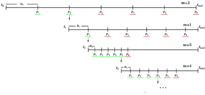
Figure 1: An illustration of how the adaptive stepsize parallel algorithm could work with $N_{CPU}=6$ processors.

The interval of $N_{CPU}$ black vertical bars is the amount of time probed by the integration using the initial step $h_{0}$. In our computations $h_{0}$ is assumed to be the total length of integration over the number of processors. A green horizontal line below a processor label indicates a successful integration, otherwise, a red line is used.

5.1 Designing the stepsize recurrence

In a given iteration we define success as obtaining an integration result with a local error below the user defined tolerance. The aim is to maximize the probability of success in each iteration, i.e., to determine the step $h_{n}$ such that it is obtained the biggest possible number of successful processors $m$ amongst the total number of available CPUs ($N_{CPU}$). We define $h_{n}$ as a function of $m$, keeping $N_{CPU}$ constant. So, if with a given integration step less than half of the processors are successful, then the next integration step needs to be smaller ($h_{n+1}<h_{n}$). Otherwise, we increase the integration step. This way, each integration becomes more efficient, both in amount of time and precision. This idea is summarized with the following expresion:

$$h_{n+1} \approx\left(\frac{2}{N_{CPU}}m+\epsilon\right)h_{n},\quad\text{for some }\epsilon>0,$$

$$=\begin{cases}\left[(1+\frac{2}{N_{CPU}}k)+\epsilon\right]h_{n}&\text{ if }m=N_{CPU}/2+k,\\ \left[(1-\frac{2}{N_{CPU}}k)+\epsilon\right]h_{n}&\text{ if }m=N_{CPU}/2-k,\\ \end{cases}$$

for some integer $k\in[0,N_{CPU}/2]$. We need $\epsilon$ to keep $h_{n+1}$ finite, even when $m=0$ and it has to be less than one for the step to always decrease in this particular case. A reasonable proposal is then, to carry the integration in half the interval when $m=0$, i.e.,

$$h_{n+1}\approx\frac{2}{N_{CPU}}mh_{n}+\frac{1}{2N_{CPU}}h_{n}\,.$$

On the other hand, if $m$ is large enough, the integration step will nearly doubles. If, for instance, this happens sequentially, for typical initial value problems there is a high probability that the next $m$ will be very small, making a poor use of the available CPUs. To avoid this, we finally propose the following recurrence:

$$h_{n+1}=\Bigg{[}\frac{2N_{CPU}-1}{(N_{CPU}+1)^{2}}m+\frac{N_{CPU}}{(2N_{CPU}-1)(N_{CPU}+1)}\Bigg{]}h_{n}\,.$$ (10)

Since $m$ is a function of $h_{n}$, this is a first order nonlinear map. It yields, $h_{n+1}>h_{n}$ if

$$m>\dfrac{(N_{CPU}+1)(2N_{CPU}^{2}-1)}{(2N_{CPU}-1)^{2}}>\frac{N_{CPU}}{2}+1\,,$$

and $h_{n+1}<h_{n}$ if

$$m<\dfrac{(N_{CPU}+1)(2N_{CPU}^{2}-1)}{(2N_{CPU}-1)^{2}}<\frac{N_{CPU}}{2}\,.$$

Moreover, $m=0$ implies $1/2>h_{n+1}/h_{n}>0$, and when $m=N_{CPU}$, then $2>h_{n+1}/h_{n}>3/4$. In consequence, this expression has the desired properties; a large integration step will ultimately lead to a low $m$ that, in turn, will decrease the stepsize and, then, increase $m$. This way, we expect $m$ to converge to the optimal value $N_{CPU}/2$.

Nevertheless, it is not desirable that the stepsize occurs to be insensitive to the given integration interval. Thus, the map $h_{n+1}(h_{n})$ was also designed to not have fixed points. Note that requiring $m\leq N_{CPU}$, implies $N_{CPU}>2$, i.e., there are not fixed points when using less than 3 CPUs. For the remaining cases, $h_{n+1}=h_{n}$ give us the condition for the map to have fixed points:

$$m=\dfrac{(N_{CPU}+1)(2N_{CPU}^{2}-1)}{(2N_{CPU}-1)^{2}}\,.$$

Let us prove that, whereas $m\in\mathbb{Z}$, the righ hand side of the above expresion is never an integer. Suppose there is a $d\in\mathbb{Z}$ such that $d|(2N_{CPU}^{2}-1)$ and $d|(2N_{CPU}-1)$ . Since $2N_{CPU}^{2}-1=(N_{CPU}+1)(2N_{CPU}-1)-N_{CPU}$ then, $d|N_{CPU}$. So, by assumption $d|[(2N_{CPU}-1)-N_{CPU}]$, leading to $d|(N_{CPU}-1)$. Therefore, considering that $d|N_{CPU}$, $d|(N_{CPU}-1)$ and $\gcd(N_{CPU},N_{CPU}-1)=1$, we conclude that $d=1$. In turn this implies $\gcd(2N_{CPU}^{2}-1,2N_{CPU}-1)=1$, and, this way, $(2N_{CPU}^{2}-1)/(2N_{CPU}-1)^{2}$ is not an integer. Thus, $(N_{CPU}+1)(2N_{CPU}^{2}-1)/(2N_{CPU}-1)^{2}$ is an integer if and only if, $(2N_{CPU}-1)^{2}|(N_{CPU}+1)$. But, recalling that $N_{CPU}>2$, then $(N_{CPU}+1)/(2N_{CPU}-1)^{2}<1$ and we get a contradiction because by definition $m\in\mathbb{Z}$. Therefore $\{h_{n}\}$ has no fixed points.

Finally, note that while increasing the value of $N_{CPU}$, $h_{0}$ becomes smaller, implying a big number of integration steps in the beginning of the process. However at a given time, since there are not fixed points, $h_{n}$ should show a bounded oscillatory behaviour around the optimal stepsize. It would imply that the proposed recurrence has an attractor, i.e., asymptotically, the process of integration will settled down around an optimal stepsize independently of its initial value. Indeed, this can be seen in figures 2 where we show some numerical realizations of $h_{n}(n)$ for different initial value problems and number of CPUs.

     

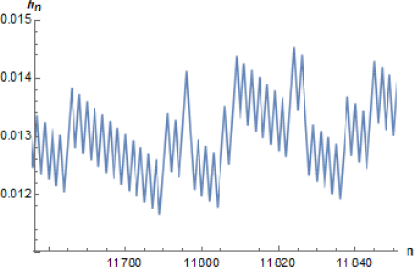
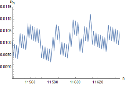
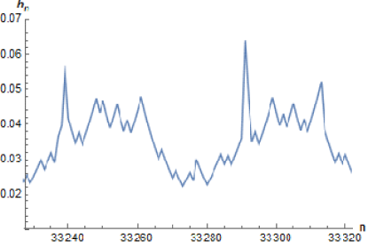
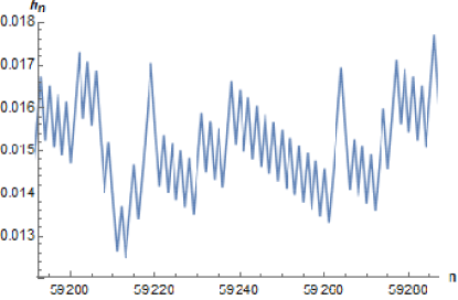
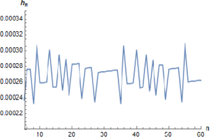
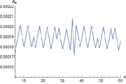
Figure 2: Oscillatory behaviour of $h_{n}$ vs $n$. Top: HH system for $N_{CPU}=10$ and $N_{CPU}=15$. Middle: HH100 system for $N_{CPU}=12$ and $N_{CPU}=14$. Right: Collapse (GC40) for 12 and 17 processors and $t=.1$.

5.2 Testing ASPA

We tested the above described algorithm by coupling it to a version of the serial DOP853. We then compared the performances of the serial DOP853 and the DOP853 with ASPA (DOP853-ASPA). With this aim we calculated the difference of the number of stepsize corrections and the difference of runtime required to reach $t=t_{end}$ as function of the tolerance for a fixed number $N_{CPU}$ of processors. We also calculated the same differences but as function of the number of processors with the tolerance fixed to $10^{-15}$. The actual values of the runtime for each case are given in correponding tables in the appendix B. In figures 3 the results for the HH problem are presented.

   

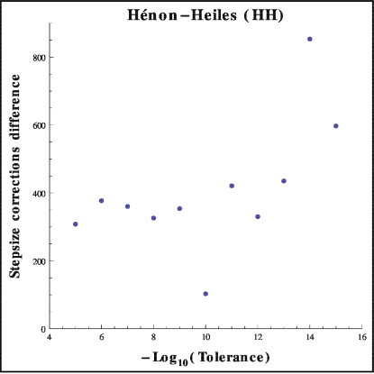
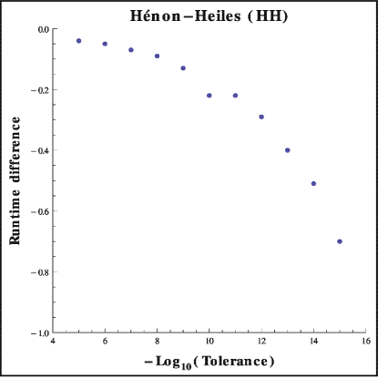
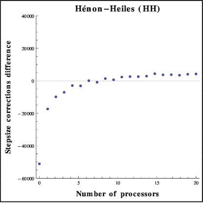
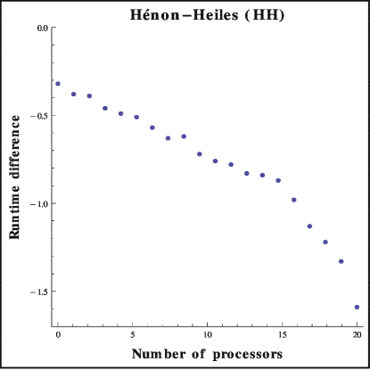
Figure 3: DOP853 minus DOP853-ASPA for HH. Left top: stepsize corrections vs tolerance. Left bottom: stepsize corrections vs number of processors. Right top: runtime vs tolerance. Right bottom: runtime vs number of processors.

Here $t_{end}=5000$ and $N_{CPU}=10$. In the two top panels we can see that, even if the DOP853 requires more stepsize corrections to reach the required tolerance, it does it in relatively less runtime. From the two bottom panels we draw the unexpected conclusion that the runtimes are comparable only when the number of stepsize corrections required by DOP853-ASPA is significantly more than that required by DOP853. This happens when using five or less processors. Moreover, notice that in the bottom panel the differences are all calculated with respect of the fixed number obtained with DOP853 (where $N_{CPU}=1$). It means that, as expected, increasing $N_{CPU}$, the number of stepsize corrections in DOP853-ASPA decreases, nevertheless, the corresponding runtime increases. All these observations hint that, when more processors are used, at each iteration the parallel overhead is more important than the time required for integration.

To determine whether this is the case, we tested the HH100 problem. The results are presented in figures 4.

   

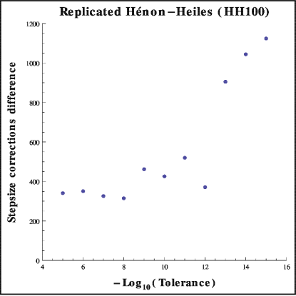
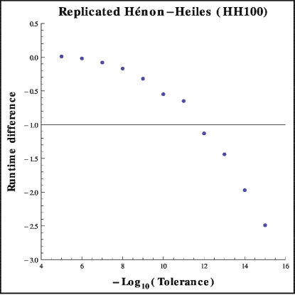
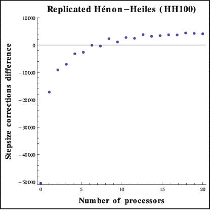
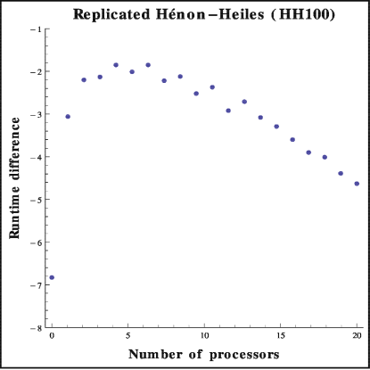
Figure 4: DOP853 minus DOP853-ASPA for HH100. Left top: stepsize corrections vs tolerance. Left bottom: stepsize corrections vs number of processors. Right top: runtime vs tolerance. Right bottom: runtime vs number of processors.

Here $t_{end}=5000$ and $N_{CPU}=10$. As in the case of HH, here DOP853 requires more stepsize corrections than DOP853-ASPA, nevertheless, for low tolerances the parallel algorithm performs slightly better than the serial. This could be due to the fact that for the HH100 problem the amount of time used for the evaluation of the RHS is comparable with the parallel overhead and that, for tolerances greater than $10^{-7}$, $N_{CPU}=10$ processors are good enough to probe the whole time interval up to $t_{end}=5000$ in very few stages.

Trying further to make the number of evaluations of the RHS to have a larger weight in the runtime, we tested the problem of the gravitational collapse, but the reduced version GC10, because the DOP853 was able to integrate it in a reasonable runtime.

In figures 5 we present the results of the comparison.

   

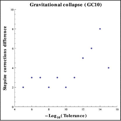
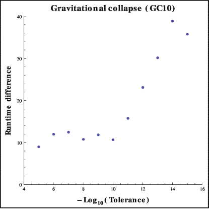
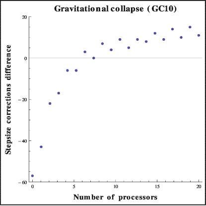
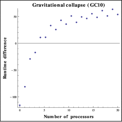
Figure 5: DOP853 minus DOP853-ASPA for GC10. Left top: stepsize corrections vs tolerance. Left bottom: stepsize corrections vs number of processors. Right top: runtime vs tolerance. Right bottom: runtime vs number of processors.

For these calculations we used $t_{end}=20$ and $N_{CPU}=20$. Now it is clear that the parallel algorithm typically performs better than the serial. From the top two panels we observe that increasing the tolerance induces a steadily increase of the difference in required stepsize corrections and this straightforwardly leads to a larger difference in runtime. The results in the bottom panels show that the DOP853-ASPA is efficient when $N_{CPU}>5$. Recalling that in the bottom panel the differences are all calculated with respect of the fixed number obtained with DOP853, we see now that increasing $N_{CPU}$ leads to less stepsize corrections required by the DOP853-ASPA, but now this also corresponds to less runtime. All the above suggests that, indeed, for the GC10 system, the parallel overhead problem is solved.

To end the comparisons, note in table 11 that for this last system, DOP853-ASPA with 5 processors lasted a little bit more than 7 minutes, while we verified that PIRK10 took about an hour to solve the same problem. On the other hand, we also checked that for GC40, DOP853-ASPA took about an hour to reach $t_{end}=0.1$ with a tolerance of $10^{-6}$, while as mentioned in section 4 PIRK10 needed about six times more (see table 4).

6 Conclusions

We tested a parallel iterated Runge–Kutta method of order 10 (PIRK10) and an adaptive stepsize parallel algorithm (ASPA), introduced in this paper, which was coupled to a Dormand–Prince method of order 8 (DOP853-ASPA). The results presented in this paper show that when the initial value problem to solve has a simple to evaluate right–hand side (as is the case in more common dynamical systems), even in the best case scenarios for the parallel methods, their performances were only comparable to the corresponding performance of a serial Dormand-Prince method of order 8 (DOP853). Therefore, taking into account code and algorithmic efficiencies, parallel integration seems to not be a good practice.

This negative result seems to be due to a parallel overhead problem, i.e., the amount of time required to coordinate parallel tasks is larger than the time required for evaluating the system right–hand side. We verified that for very complex initial value problems or low tolerances the parallel methods can outperform DOP853. For instance, such systems arise while using Galerkin projection to solve systems of partial differential equations or when simulating multi–agent systems. In these cases, it seems to be more efficient to parallelize the search for an optimal stepsize for integration than to parallelize the integration scheme. Indeed, our method, DOP853-ASPA, consistently outperformed PIRK10 by almost an order of runtime. Moreover, even in some cases where DOP853 did a better job than PIRK10, our method was able to solve the corresponding initial value problem in less time than both these methods.

A nice feature of ASPA is that it does not relies on a given core integrator, it can be coupled to any method with a scheme to estimate the local integration error. It can even be another parallel method more efficient than the one tested here.

Appendix A Butcher tableau

Butcher tableau for an implicit Runge–Kutta method of order $10$ ref. [10].

$$\begin{array}[]{c|c c c c c}\frac{1}{2}-\omega_{2}&\omega_{1}&\omega_{1}^{\prime}-\omega_{3}+\omega_{4}^{\prime}&\frac{32}{225}-\omega_{5}&\omega_{1}^{\prime}-\omega_{3}-\omega_{4}^{\prime}&\omega_{1}-\omega_{6}\\[7.11317pt] \frac{1}{2}-\omega_{2}^{\prime}&\omega_{1}-\omega_{3}^{\prime}+\omega_{4}&\omega_{1}^{\prime}&\frac{32}{225}-\omega_{5}^{\prime}&\omega_{1}^{\prime}-\omega_{6}^{\prime}&\omega_{1}-\omega_{3}^{\prime}-\omega_{4}\\[7.11317pt] \frac{1}{2}&\omega_{1}+\omega_{7}&\omega_{1}^{\prime}+\omega_{7}^{\prime}&\frac{32}{225}&\omega_{1}^{\prime}-\omega_{7}^{\prime}&\omega_{1}-\omega_{7}\\[7.11317pt] \frac{1}{2}+\omega_{2}^{\prime}&\omega_{1}+\omega_{3}^{\prime}+\omega_{4}&\omega_{1}^{\prime}+\omega_{6}^{\prime}&\frac{32}{225}+\omega_{5}^{\prime}&\omega_{1}^{\prime}&\omega_{1}+\omega_{{}^{3}}^{\prime}-\omega_{4}\\[7.11317pt] \frac{1}{2}+\omega_{2}&\omega_{1}+\omega_{6}&\omega^{\prime}_{1}+\omega_{3}+\omega_{4}^{\prime}&\frac{32}{225}+\omega_{5}&\omega^{\prime}_{1}+\omega_{3}-\omega^{\prime}_{4}&\omega_{1}\\[7.11317pt] \hline\cr\\[-7.11317pt] &2\omega_{1}&2\omega_{1}^{\prime}&\frac{64}{225}&2\omega_{1}^{\prime}&2\omega_{1}\\ \end{array}$$

Table 5: 5-stage, order 10.

where the $\omega_{i}$ are given by,

$$\omega_{1}=\frac{322-13\sqrt{70}}{3600},\quad\omega_{1}^{\prime}=\frac{322+13\sqrt{70}}{3600},$$

$$\omega{2}=\frac{1}{2}\sqrt{\frac{35+2\sqrt{70}}{63}},\quad\omega{2}^{\prime}=\frac{1}{2}\sqrt{\frac{35-2\sqrt{70}}{63}},$$

$$\omega{3}=\omega_{2}\frac{452+59\sqrt{70}}{3240},\quad\omega^{\prime}_{3}=\omega^{\prime}_{2}\frac{452-59\sqrt{70}}{3240},$$

$$\omega_{4}=\omega_{2}\frac{64+11\sqrt{70}}{1080},\quad\omega^{\prime}_{4}=\omega^{\prime}_{2}\frac{64-11\sqrt{70}}{1080},$$

$$\omega_{5}=8\omega_{2}\frac{23-\sqrt{70}}{405},\quad\omega^{\prime}_{5}=8\omega^{\prime}_{2}\frac{23+\sqrt{70}}{405},$$

$$\omega_{6}=\omega_{2}-2\omega_{3}-\omega_{5},\quad\omega^{\prime}_{6}=\omega^{\prime}_{2}-2\omega^{\prime}_{3}-\omega^{\prime}_{5},$$

$$\omega_{7}=\omega_{2}\frac{308-23\sqrt{70}}{960},\quad\omega^{\prime}_{7}=\omega^{\prime}_{2}\frac{308+23\sqrt{70}}{960}.$$

Appendix B Runtimes

	DOP853-ASPA		DOP853
T	stepsize corrections	Time	stepsize corrections	Time
5	4333	0.06	4641	0.09
6	5778	0.07	6155	0.02
7	7826	0.1	8186	0.03
8	10520	0.12	10846	0.03
9	14040	0.17	14394	0.04
10	18825	0.27	18928	0.05
11	24876	0.29	25297	0.07
12	33327	0.38	33657	0.09
13	49989	0.52	45424	0.12
14	59292	0.67	60145	0.12
15	79393	0.91	79990	0.21

Table 6: $T=-\log_{10}(tolerance)$. HH system using 10 processor and final time 5000.

	DOP853-ASPA		DOP853
CPU’s	stepsize corrections	Time	stepsize corrections	Time
1	131089	0.53	79990	0.21
2	97312	0.59	-	-
3	89886	0.6	-	-
4	87133	0.67	-	-
5	82941	0.7	-	-
6	83143	0.72	-	-
7	79923	0.78	-	-
8	80891	0.84	-	-
9	78640	0.83	-	-
10	79393	0.93	-	-
11	77713	0.96	-	-
12	77428	0.99	-	-
13	77469	1.04	-	-
14	77170	1.05	-	-
15	75664	1.1	-	-
16	76341	1.19	-	-
17	76243	1.33	-	-
18	76566	1.43	-	-
19	75997	1.54	-	-
20	75799	1.8	-	-

Table 7: HH system using tolerance $10^{-15}$.

	DOP853-ASPA		DOP853
T	stepsize corrections	Time	stepsize corrections	Time
5	4321	0.74	4662	0.75
6	5853	1.01	6204	0.99
7	7844	1.34	8170	1.26
8	10499	1.79	10814	1.62
9	13829	2.35	14291	2.03
10	18660	3.16	19086	2.61
11	24902	4.22	25422	3.57
12	33369	5.66	33740	4.53
13	44362	7.53	45267	6.09
14	59127	10.07	60171	8.27
15	79444	13.45	80568	10.96

Table 8: $T=-\log_{10}(tolerance)$. HH100 system. Here we used 10 processors and final time 5000.

	DOP853-ASPA		DOP853
CPU’s	stepsize corrections	Time	stepsize corrections	Time
1	131089	17.79	80568	10.96
2	97765	14.02	-	-
3	89631	13.16	-	-
4	87586	13.09	-	-
5	83745	12.81	-	-
6	83174	12.97	-	-
7	80635	12.81	-	-
8	80946	13.18	-	-
9	78234	13.08	-	-
10	79444	13.48	-	-
11	77802	13.33	-	-
12	78105	13.88	-	-
13	76761	13.67	-	-
14	77358	14.04	-	-
15	77139	14.25	-	-
16	76813	14.56	-	-
17	76853	14.86	-	-
18	76150	14.97	-	-
19	76295	17.33	-	-
20	76440	15.59	-	-

Table 9: HH100 system.

	DOP853-ASPA		DOP853
T	stepsize corrections	Time	stepsize corrections	Time
5	7	17.39	9	26.37
6	10	24.82	13	36.79
7	15	37.25	18	49.71
8	22	54.65	24	65.42
9	30	74.45	33	86.28
10	42	104.37	44	115.03
11	57	141.7	60	157.45
12	75	186.07	80	209.17
13	102	253.1	108	283.24
14	136	337.85	144	376.71
15	189	469.16	193	504.9

Table 10: $T=-\log_{10}(tolerance)$. Collapse (GC10) using 10 processors and final time 20.

	DOP853-ASPA		DOP853
CPU’s	stepsize corrections	Time	stepsize corrections	Time
1	250	620.75	193	504.9
2	236	586.12	-	-
3	215	534.19	-	-
4	210	522.19	-	-
5	199	494.1	-	-
6	199	493.71	-	-
7	190	471.84	-	-
8	193	479.29	-	-
9	186	462.08	-	-
10	189	469.16	-	-
11	184	453.94	-	-
12	188	465.82	-	-
13	184	455.71	-	-
14	185	458.62	-	-
15	181	449.76	-	-
16	184	456.48	-	-
17	179	443.96	-	-
18	183	453.85	-	-
19	178	441.52	-	-
20	182	451.2	-	-

Table 11: GC10 using tolerance $10^{-15}$ and final time 20.

References

- [1] Boyd, John P. ”Chebyshev and Fourier Spectram Methods”. Dover, New York (2001), 688 pp.
- [2] Wooldridge, M. J. ”An introduction to multiagent systems”. New York, NY: Wiley (2002).
- [3] Burrage, Kevin. ”Parallel and sequential methods for ordinary differential equations”. Clarendon Press, 1995.
- [4] Van Der Houwen, P.J.; Sommeneijer, B.P., ”Parallel Iteration of High-Order Runge–Kutta Methods with Stepsize Control”, Journal of Computational and Applied Mathematics.
- [5] Hairer, Ernst; Nørsett, Syvert Paul; Wanner, Gerhard (2008), ”Solving ordinary differential equations I: Nonstiff problems”, Berlin, New York: Springer-Verlag, ISBN 978-3-540-56670-0.
- [6] Dormand, J.R.; Prince, P.J., ”A family of embedded Runge–Kutta formulae”, Journal of Computational and Applied Mathematics, Volume 6, Issue 1, March 1980, Pages 19–26 http://dx.doi.org/10.1016/0771-050X(80)90013-3
- [7] http://www.unige.ch/ hairer/software.html
- [8] Hénon, M.; Heiles, C. (1964). ”The applicability of the third integral of motion: Some numerical experiments”. The Astrophysical Journal 69: 73–79.
- [9] de Oliveira, H. P.; Pando Zayas, L. A.; Terrero-Escalante, C. A., “Turbulence and Chaos in Anti-de-Sitter Gravity,” Int. J. Mod. Phys. D 21, 1242013 (2012) [arXiv:1205.3232 [hep-th]].
- [10] Butcher, J.C., ”Implicit Runge–Kutta Processes”, American Mathematical Society, January 1964, Pages 50-64.