Dynamics of stochastic approximation with iterate-dependent Markov noise under verifiable conditions in compact state space with the stability of iterates not ensured

Abstract

This paper compiles several aspects of the dynamics of stochastic approximation algorithms with Markov iterate-dependent noise when the iterates are not known to be stable beforehand. We achieve the same by extending the lock-in probability (i.e. the probability of convergence of the iterates to a specific attractor of the limiting o.d.e.  given that the iterates are in its domain of attraction after a sufficiently large number of iterations (say) $n_{0}$) framework to such recursions. Specifically, with the more restrictive assumption of Markov iterate-dependent noise supported on a bounded subset of the Euclidean space we give a lower bound for the lock-in probability. We use these results to prove almost sure convergence of the iterates to the specified attractor when the iterates satisfy an asymptotic tightness condition. The novelty of our approach is that if the state space of the Markov process is compact we prove almost sure convergence under much weaker assumptions compared to the work by Andrieu et al. which solves the general state space case under much restrictive assumptions. We also extend our single timescale results to the case where there are two separate recursions over two different timescales. This, in turn, is shown to be useful in analyzing the tracking ability of general adaptive algorithms. Additionally, we show that our results can be used to derive a sample complexity estimate of such recursions, which then can be used for step-size selection.

I Introduction

Stochastic approximation algorithms are sequential non-parametric methods for finding a zero or minimum of a function in cases where only the noisy observations of the function values are available. Stochastic approximation iterates in $\mathbb{R}^{d}$ are given by

$$\theta_{n+1}=\theta_{n}+a(n)f(\theta_{n},Y_{n+1}),n\geq 0,$$ (1)

where $\theta_{0}$ is the initial point, $\{\theta_{n}\}$ are the iterates, $\{Y_{n}\}$ is an $\mathbb{R}^{d}$- valued ‘Markov iterate-dependent’ noise sequence, i.e., it satisfies

$$P[Y_{n+1}\in A|\mathcal{F}_{n}]=\int_{A}\Pi_{\theta_{n}}(Y_{n};dx)\ \mbox{a.s.,}~{}\forall n,$$ (2)

where $\mathcal{F}_{n}:=$ the $\sigma$-field generated by all random variables realized till time $n$ and $a(n)$ is the $n$-th step-size.

It is well known that under reasonable assumptions [1], [2], (1) asymptotically tracks the o.d.e.

$$\dot{\theta}(t)=h(\theta(t)),$$ (3)

where $h(\theta)=\int f(\theta,y)\Gamma_{\theta}(dy)$, with $\Gamma_{\theta}$ being the unique stationary distribution of the Markov iterate-dependent process $\{Y_{n}\}$ for a fixed $\theta$. Among them the most important assumption is the stability of the iterates, i.e.,

$$\sup_{n}\|\theta_{n}\|<\infty\ a.s.$$ (4)

In literature sufficient conditions that guarantee (4) are available (e.g. based on a Lyapunov function [3, Chap. 6.7], [4] etc. As mentioned in [4], proving stability of the iterates is a tedious task with the Markovian dynamic due to the noise term $f(\theta_{n},Y_{n+1})-h(\theta_{n})$. In [6], the truncations on adaptive truncation sets from [7] has been extended to the case where the noise is Markov. It is clearly mentioned there that the procedure they follow is different in some respects from the original procedure proposed by [7]. To prove that the number of re-initializations of the procedure described in [6, Section 3.2] is finite, they establish a bound on the probability that the $n$-th reinitialization time is finite in terms of the fluctuations of the noise sequence of the algorithm between successive re-initializations. Although the results are described for Markov processes taking values in a general state space (Polish) some of the assumptions therein are restrictive such as the assumptions on global Lyapunov function (see (A1) in [6]). Additionally, in order to control the fluctuations some less classical assumptions have been imposed on the transition kernel (regularity properties in $V$ and $V^{p}$ norm) as well as on the vector field $g(\cdot,\cdot)$ (see (DRI2) and (DRI3)) and the discussion thereafter.

In this work, we investigate the dynamics of stochastic approximation with Markov iterate-dependent noise when (4) is not known to be satisfied beforehand. We achieve the same by extending the lock-in probability framework of Borkar [8] to such a recursion, leading in turn to the following:

1. Let $H$ be an asymptotically stable attractor of (3) and $G$ be its domain of attraction. If $\{\theta_{n}\}$ is asymptotically tight (which is a much weaker condition than (4)) and $\liminf_{n}P(\theta_{n}\in G)=1,$ then $P(\theta_{n}\to H)=1$ under a reasonable set of assumptions seem to be routinely satisfied in applications such as reinforcement learning [9]. To the best of our knowledge this is the first time an almost sure convergence proof for such a recursion is presented without assuming stability of the iterates, however following the classic Poisson equation model of Metivier and Priouret [1] for such recursion which is designed keeping in mind the stability of the iterates. Additionally, a simple test for asymptotic tightness is also provided. Our tightness condition does not assume existence of a quadratic Lyapunov function as with [10] as they work mainly when the vector field is linear. Also, we show that for linear stochastic approximation our tightness condition always gets satisfied in the case of a finite state Markov chain.

2. We show that under some reasonable assumptions for common step-size sequences such as $\{\frac{1}{n^{k}}\},\frac{1}{2}<k\leq 1$ and $\frac{1}{n(\log n)^{k}},k\leq 1$, if the iterates belong to some special open set with compact closure in the domain of attraction of the local attractor infinitely often w.p. 1, then the iterates are stable and converge a.s. to the local attractor.

3. We show that our results can be used to analyze the tracking ability of general (not necessarily linear) stochastic approximation driven by another “slowly” varying stochastic approximation process when the iterates are not known to be stable. This involves extending the lock-in probability results to the case with two iterates evolving along different timescales. Such results are useful in the context of adaptive algorithms [11] as not much is known about the stability of frameworks with different timescales. Note that in two time-scale stochastic approximation the coupled o.d.e has no attractor. Also, to prove the convergence of the coupled iterates stability of the slower iterate is necessary. Therefore we need to consider two quantities describing difference (over compact time interval) between the algorithm and the o.d.e., one for the coupled algorithm/o.d.e and another for the slower algorithm/o.d.e. This gives rise to a situation where the conditioning event in the martingale concentration inequality does not belong to the first $\sigma$-field in the current collection of $\sigma$-fields (unlike in the case of single timescale stochastic approximation where the conditioning event always belongs to the first $\sigma$-field in the current collection of $\sigma$-fields [5, p 40]).

   Such results are useful in the context of adaptive algorithms [11] as not much is known about the stability of frameworks with different timescales. There is some recent work [12] that also estimates the lock-in probability for multiple timescales, however, under the assumption that the vector fields are “linear”.

4. We derive a sample complexity estimate (explained later) for such a recursion.

The motivation for lock-in probability comes from a phenomenon noticed by W.B.Arthur in simple urn models ([5, Chap. 1]) of increasing return economics: if occurrences predominantly of one type tend to fetch more occurrences of the same type, then after some initial randomness the process gets locked into that possibly undesirable type of occurrence. Moreover, it is known that under reasonable conditions, every asymptotically stable equilibrium will have a positive probability of emerging as $\lim_{n\to\infty}\theta_{n}$ [13], while this probability is zero for unstable equilibria under mild conditions on the noise [14, 15].

With this picture in mind and to give a quantitative explanation of this phenomenon, Borkar defined lock-in probability [8] for iterates of the form

$$\theta_{n+1}=\theta_{n}+a(n)(h(\theta_{n})+M_{n+1}),$$ (5)

where $\{M_{n}\}$ constitutes martingale noise, i.e., a martingale difference sequence, as the probability of convergence of $\theta_{n}$ to an asymptotically stable attractor $H$ of (3) given that the iterate is in a neighbourhood $B$ thereof after a sufficiently large $n_{0}$, i.e.,

$$P(\theta_{n}\to H|\theta_{n_{0}}\in B)$$

for a compact $B\subset G$. He also found a lower bound for this quantity by studying the local behavior of iterates in a neighborhood of the attractor. Clearly, $n_{0}$ depends on the particular $H$. Specifically, under the assumption $E[\|M_{n+1}\|^{2}|\mathcal{F}_{n}]\leq K(1+\|\theta_{n}\|^{2})\mbox{~{}a.s.}$ the bound obtained is $1-O(\sum_{i\geq n_{0}}a(i)^{2})$ and under the more restrictive condition $\|M_{n+1}\|\leq K_{0}(1+\|\theta_{n}\|)\mbox{~{}a.s.}$, a tighter bound of $1-O(e^{-\frac{1}{\sum_{i\geq n_{0}}a(i)^{2}}})$ has been obtained [8]. There are recent results [16, 10] which obtain tighter bound under much weaker assumptions on martingale and step-size sequence.

The fact that lock-in probability is not just a theoretical quantity to explain the lock-in phenomenon of information economics was shown by Kamal [10]. If the iterates are tight then lock-in probability results are used in [10] to prove almost sure convergence of the stochastic approximation recursion (with only martingale difference noise) to the global attractor.

The phenomenon described earlier can be observed in reinforcement learning (RL) applications where the limiting o.d.e. has multiple equilibria, e.g., with several instances of stochastic gradient descent in machine learning. We extend in this paper the currently available lock-in probability estimates to the case where the vector field includes a Markov iterate-dependent noise. This is for instance the case with many reinforcement learning algorithms where Markov iterate-dependent noise arises naturally because of the Markov decision process in the background.

Although the recursion (1) covers most of the cases of stochastic approximation with Markov iterate-dependent noise, there are reinforcement learning scenarios where there can be a dependence on both the present and the next sample of the Markov iterate-dependent noise in the vector field [17]. For such scenarios the general recursion is:

$$\theta_{n+1}=\theta_{n}+a(n)f(\theta_{n},Y_{n},Y_{n+1}).$$ (6)

One can write (6) as

$$\theta_{n+1}=\theta_{n}+a(n)\left[E[f(\theta_{n},Y_{n},Y_{n+1})|\mathcal{F}_{n}]+M_{n+1}\right],$$

where $\mathcal{F}_{n}=\sigma(\theta_{m},Y_{m},m\leq n)$ and $M_{n+1}=f(\theta_{n},Y_{n},Y_{n+1})-E[f(\theta_{n},Y_{n},Y_{n+1})|\mathcal{F}_{n}]$ is a martingale difference sequence. Therefore, with abuse of notation, the general recursion which takes care of Markov iterate-dependent noise can be described as

$$\theta_{n+1}=\theta_{n}+a(n)\left[f(\theta_{n},Y_{n})+M_{n+1}\right].$$ (7)

In fact, this also covers the situation where both Markov iterate-dependent and martingale difference noise sequences are present. In this work, we give a lower bound on the lock-in probability estimate of iterates of the form (7) using the Poisson equation based analysis as in [1, 2]. Under some assumptions in [1] and some further assumptions, we get a lower bound of $1-O(e^{-\frac{C}{\sum_{i=n_{0}}^{\infty}a(i)^{2}}})$ for the recursion (7), and thus also for the special case (1). Therefore, with the more general assumption of Markov iterate-dependent noise, we recover the same bounds available for the setting of martingale noise [5, p. 38] although with some additional assumptions on the Markov iterate-dependent process and step size sequence.

Very few results [18] are available on non-asymptotic rate of convergence of general stochastic approximation iterates (1), see also [19] for stochastic gradient descent. But lock-in probability estimates can be used to calculate an upper bound for the sample complexity estimate of stochastic approximation [5, chap. 4.2],[10]. Given a desired accuracy $\epsilon>0$ and confidence $\gamma$, the sample complexity estimate is defined to be the minimum number of iterations $N(\epsilon,\gamma)$ after which the iterates are within a certain neighbourhood (which is a function of $\epsilon$) of $H$ with probability at least $1-\gamma$. This is slightly different from the sample complexity estimate arising in the context of consistent supervised learning algorithms in statistical learning theory [20]. The reasons are:

1. In the case of statistical learning theory, sample complexity corresponds to the number of i.i.d training samples needed for the algorithm to successfully learn a target function. However, in our case, we have a recursive scheme whose sample complexity depends on the step-size.

2. Ours is a conditional estimate, i.e., the estimate is conditioned on the fact that $\theta_{n_{0}}\in B$ where $B$ is an open subset of the domain of attraction of $H\subset B$ and has compact closure, and $n_{0}$ is sufficiently large.

Another point worth noting is that sample complexity results are much weaker than lock-in probability and do not require existence of Lyapunov function. In our work, we give a sample complexity estimate for the setting where the recursion is a stochastic fixed point iteration driven by a Markov iterate-dependent noise. This shows a quantitative estimate of large vs. small step size trade-off well known in stochastic approximation literature that is shown to be useful in choosing the optimal step-size.

The organization of the paper is as follows: Section II formally defines the problem and provides background and assumptions. Section III presents our lock-in probability results for single timescale stochastic approximation. Section IV presents results on almost sure convergence to a local attractor using our results along with the assumption of asymptotic tightness of the iterates. Moreover, this section shows that stability of the iterates can be proved using our results. Section V gives an estimate of the lock-in probability for iterates evolving along different timescales and analyzes the tracking ability of adaptive algorithms using these results. Section VI describes the results on sample complexity. Finally, we conclude by providing some future research directions.

II The Problem and Assumptions

In the following we describe the preliminaries and notation that we use in our proofs. Most of the definitions and notation are from [1, 5, 10]. The notations used for ordinary differential equations are similar to [5, Appendix 11.2]. In the following we describe the lock-in probability settings based on the approach in [1]. The main idea is to assume existence of a solution to the Poisson equation (Assumption (M4) from Section III B of [1]), thus converting Markov iterate-dependent noise into a martingale difference sequence and with additional additive errors. We refer the readers to [2, Part II,Chap. 2, Theorem 6], [1, Section III D, Appendix A] for details on the existence and properties of solution of the Poisson equation for a Markov iterate-dependent process.

In this work we prove almost sure convergence for recursion (7) without assuming stability of the iterates, however, following the classic Poisson equation model stated above where the assumptions are designed keeping in mind the stability of the iterates. To make up for this we need to strengthen some existing assumptions of [1] (shown next), these are standard assumptions satisfied in application areas such as reinforcement learning.

Let $G\subset\mathbb{R}^{d}$ be open and let $V:G\to[0,\infty)$ be such that $\langle\nabla V,h\rangle:G\to\mathbb{R}$ is non-positive. We shall assume as in [5] that $H:=\{\theta:V(\theta)=0\}$ is equal to the set $\{\theta:\langle\nabla V(\theta),h(\theta)\rangle=0\}$ and is a compact subset of $G$. Thus, $V$ is a strict Lyapunov function. Then $H$ is an asymptotically stable invariant set of the differential equation $\dot{\theta}(t)=h(\theta(t))$. Let there be an open set $B$ with compact closure such that $H\subset B\subset\bar{B}\subset G$. In this setting, the lock-in probability is defined to be the probability that the sequence $\{\theta_{n}\}$ is convergent to $H$, conditioned on the event that $\theta_{n_{0}}\in B$ for some $n_{0}$ sufficiently large.

Recall from Theorem 8 of [5, p. 37] that for the case of martingale difference noise, $\mathbb{P}[\theta_{n}\rightarrow H|\theta_{n_{0}}\in B]\geq 1-O(e^{-\frac{1}{s(n_{0})}}),$ where $s(n_{0}):=\sum_{m=n_{0}}^{\infty}a(m)^{2}$. In this paper we obtain these results when the noise is Markov iterate-dependent under the following assumptions:

1. $\limsup_{n\to\infty}\|Y_{n}\|<\bar{C}$ a.s. for some $\bar{C}>0$. This is stronger than $\limsup_{n}E[\|Y_{n}\|^{2}]<\infty$ which is implied by (M2) of [1].

2. $\sup_{y}\|f(\theta,y)\|\leq K(1+\|\theta\|)$ for all $\theta$.

   Remark 1.

   (A2) is a standard assumption satisfied in reinforcement learning scenarios as pointed in [8, p 6]. Clearly, this is stronger than the hypothesis (F) on $f$ as mentioned in [1, p 143].

3. The stepsizes $\{a(n)\}$ are non-increasing positive scalars satisfying

   $$\sum_{n}a(n)=\infty,\sum_{n}{a(n)}^{2}<\infty.$$

4. For every $\theta$, the Markov chain $\Pi_{\theta}$ has a unique invariant probability $\Gamma_{\theta}$. ((M1) from [1]). Further, $h(\theta)=\int f(\theta,y)\Gamma_{\theta}(dy)$ is Lipschitz continuous in $\theta$ with Lipschitz constant $0<L<\infty$.

5. $\|M_{n+1}\|\leq K^{\prime}(1+\|\theta_{n}\|)$ a.s. $\forall n$. Note that in [1] there was no martingale noise.

6. For every $\theta$ the Poisson equation

   $$(1-\Pi_{\theta})v_{\theta}=f(\theta,\cdot)-\int f(\theta,y)\Gamma_{\theta}(dy)$$

   has a solution $v_{\theta}$. This is (M4) from [1]. Here $\Pi_{\theta}\phi(x):=\int\Pi_{\theta}(x;dy)\phi(y)$.

7. For all $R>0$ there exist constants $C_{R}>0$ such that

   1. $\sup_{\|\theta\|\leq R}\|v_{\theta}(x)\|\leq C_{R}(1+\|x\|)$.

   2. $\|v_{\theta}(x)-v_{\theta^{\prime}}(x)\|\leq C_{R}\|\theta-\theta^{\prime}\|(1+\|x\|)$ for all $\|\theta\|\leq R$, $\|\theta^{\prime}\|\leq R$.

   This is (M5)b,c from [1].

Under the above assumptions we shall show that

$$\mathbb{P}\left[\theta_{n}\rightarrow H|\theta_{n_{0}}\in B\right]\geq 1-O\left(e^{-\frac{c}{s(n_{0})}}\right)$$

for sufficiently large $n_{0}$.

We provide a more detailed discussion on assumptions (A1) and (A2) as well as possible relaxations of these in Section III-A. Additionally, we give a detailed comparison of our assumptions with the assumptions of [6] in Section IV-C.

III Lock-in probability calculation for single timescale stochastic approximation

In this subsection we give a lower bound for $\mathbb{P}[\theta_{n}\rightarrow H|\theta_{n_{0}}\in B]$ in terms of $s(n_{0})$ when $n_{0}$ is sufficiently large based on the settings described in Section II. How large $n_{0}$ needs to be will be specified soon. Before proceeding further we describe our notations and recall some known results. For $\delta>0$, $N_{\delta}(A)$ for a set $A$ denotes its $\delta$-neighborhood $\{y:\|y-x\|<\delta,\forall\ x\in A\}$. Let $H^{a}:=N_{a}(H)$. Fix some $0<\epsilon_{1}<\epsilon$ and $\delta_{B}>0$ such that $N_{\delta_{B}}(H^{\epsilon_{1}})\subset H^{\epsilon}\subset B$.

Let $T$ be an upper bound for the time required for a solution of the o.d.e. (3) to reach the set $H^{\epsilon_{1}}$, starting from an initial condition in $\bar{B}$. The existence of such a $T$ independent of the starting point in $\bar{B}$ can be proved using the continuity of flow of the o.d.e (3) around the initial point and the fact that $H$ is an asymptotically stable set of the same o.d.e; see Lemma 1 of [5, Chap. 3] for the proof of a similar result.

Remark 2.

Due to the above argument we do not need assumption (A4) from [16] and similar assumption made in [5, p 32]. They clearly gets satisfied if the vector field is linear, however for nonlinear stochastic approximation it is not clear whether they gets satisfied.

Let $t(n)=\sum_{m=0}^{n-1}a(m)$, $n\geq 1$ with $t(0)=0$. Let $n_{0}\geq 0,n_{m}=\min\{n:t(n)\geq t(n_{m-1})+T\}$ and $T_{m}=t(n_{m})$, $m\geq 1$. Define $\bar{\theta}(t)$ by: $\bar{\theta}(t(n))=\theta_{n}$, with linear interpolation on $[t(n),t(n+1))$ for all $n$. Let $\theta^{t(n_{m})}(\cdot)$ be the solution of the limiting o.d.e. (3) on $[t(n_{m}),t(n_{m+1}))$ with the initial condition $\theta^{t(n_{m})}(t(n_{m}))=\bar{\theta}(t(n_{m}))=\theta_{n_{m}}$. Let

$$\rho_{m}:=\sup_{t\in[t(n_{m}),t(n_{m+1}))}\|\bar{\theta}(t)-\theta^{t(n_{m})}(t)\|.$$

We recall here a few key results from [8]. As shown there, if $\theta_{n_{0}}\in B$, and $\rho_{m}<\delta_{B}$ for all $m\geq 0$, then $\bar{\theta}(T_{n})$ is in $H^{\epsilon}\subset B$ for all $n\geq 1$. Therefore using discrete Gronwall’s inequality we can show that $\sup_{t\geq T_{0}}\bar{\theta}(t)<\infty$. It is also known ([1], section IIC) that if the sequence of iterates $\{\theta_{n}\}$ remains bounded almost surely on a prescribed set of sample points, and if on this set the iterates lie in a compact set in the domain of attraction of any local attractor infinitely often then the sequence of iterates converge almost surely on this set to that local attractor. Using this fact gives the following estimate on the probability of convergence, conditioned on $\theta_{n_{0}}\in B$ ([5], Lemma 1, p. 33):

$$P\left[\bar{\theta}(t)\rightarrow H|\theta_{n_{0}}\in B\right]\geq P\left[\rho_{m}<\delta_{B}\ \forall m\geq 0|\theta_{n_{0}}\in B\right].$$

Let $\mathcal{B}_{m}$ denote the event that $\theta_{n_{0}}\in B$ and $\rho_{k}<\delta_{B}$ for $k=0,1,\ldots,m$. Clearly, $B_{m}\in\mathcal{F}_{n_{m+1}}$. The following lower bound for the above probability has been obtained in ([5], Lemma 2, p. 33):

$$P\left[\rho_{m}<\delta_{B}\ \forall m\geq 0|\theta_{n_{0}}\in B\right]\geq 1-\sum_{m=0}^{\infty}P\left[\rho_{m}\geq\delta_{B}|\mathcal{B}_{m-1}\right].$$

Subsequently the idea is to find an upper bound for $\rho_{m}$ consisting of errors (asymptotically negligible on $\mathcal{B}_{m-1}$) as well as martingale terms. Then for some large $n_{0}$, one may bound $P(\rho_{m}\geq\delta_{B}|\mathcal{B}_{m-1})$ using a suitable martingale concentration inequality. In the following we describe how to achieve the above in our setting.

Using the Poisson equation one can write the recursion (7) as

$$\theta_{n+1}=\theta_{n}+a(n)h(\theta_{n})+a(n)\left[v_{\theta_{n}}(Y_{n})-\Pi_{\theta_{n}}v_{\theta_{n}}(Y_{n})+M_{n+1}\right]$$

where $\Pi_{\theta}\phi(x)=\int\phi(y)\Pi_{\theta}(x;dy)$. Let $\zeta_{n+1}=v_{\theta_{n}}(Y_{n})-\Pi_{\theta_{n}}v_{\theta_{n}}(Y_{n})$. We decompose

$$\begin{aligned} \zeta_{n+1}=v_{\theta_{n}}(Y_{n+1})-\Pi_{\theta_{n}}v_{\theta_{n}}(Y_{n})+v_{\theta_{n}}(Y_{n})-v_{\theta_{n+1}}(Y_{n+1})+\\ v_{\theta_{n+1}}(Y_{n+1})-v_{\theta_{n}}(Y_{n+1})\end{aligned}$$

and set

$$A_{n}=\sum_{k=0}^{n-1}a(k)\zeta^{(1)}_{k+1},\ B_{n}=\sum_{k=0}^{n-1}a(k)\zeta^{(2)}_{k+1},\ C_{n}=\sum_{k=0}^{n-1}a(k)\zeta^{(3)}_{k+1},$$

$$D_{n}=\sum_{k=0}^{n-1}a(k)M_{k+1},n\geq 1$$

where

$$\zeta^{(1)}_{n+1}=v_{\theta_{n}}(Y_{n+1})-\Pi_{\theta_{n}}v_{\theta_{n}}(Y_{n}),\ \zeta^{(2)}_{n+1}=v_{\theta_{n}}(Y_{n})-v_{\theta_{n+1}}(Y_{n+1}),$$

$$\zeta^{(3)}_{n+1}=v_{\theta_{n+1}}(Y_{n+1})-v_{\theta_{n}}(Y_{n+1}).$$

Then one can easily see that as in the proof of Lemma 3 of [5, p. 34]

$$\rho_{m}\leq (Ca(n_{0})+K_{T}CLs(n_{0}))+K_{T}[\max_{n_{m}\leq j\leq n_{m+1}}\|A_{j}-A_{n_{m}}\|+$$

$$\max_{n_{m}\leq j\leq n_{m+1}}\|B_{j}-B_{n_{m}}\|+\max_{n_{m}\leq j\leq n_{m+1}}\|C_{j}-C_{n_{m}}\|+$$

$$\max_{n_{m}\leq j\leq n_{m+1}}\|D_{j}-D_{n_{m}}\|],$$ (8)

where $C$ is a bound on $\|h(\Phi_{t}(\theta)\|$, with $\Phi_{t}$ being the time-$t$ flow map for the o.d.e (3), $0\leq t\leq T+1$ and $\theta\in\bar{B}$. Also, $K_{T}=e^{LT}$.

Choose an $n_{0}^{(1)}$ such that

$$(Ca(n_{0}^{(1)})+K_{T}CLs(n_{0}^{(1)}))<\delta_{B}/2.$$ (9)

The following important lemma shows that $\forall m\geq 1$, on $\mathcal{B}_{m-1}$, the iterates (7) are stable over $T$-length interval with the stability constant independent of $m$. This is enough for our proofs to go through and justifies the importance of assumptions (A2) and (A5).

Lemma III.1.

On $\mathcal{B}_{m-1},\|\theta_{j}\|\leq K^{\prime\prime}$ for any $n_{m}\leq j\leq n_{m+1}$ where the constant $K^{\prime\prime}$ is independent of $m$.

Proof.

From the definition of $\mathcal{B}_{m-1}$, we know that $\theta_{n_{m}}\in B$ on this event. Let $\|\theta_{n_{m}}\|\leq\tilde{C}$ $\forall m$. Clearly, for $n_{m}\leq j\leq n_{m+1}$,

$$\begin{aligned} \|\theta_{j}\|&\leq\|\theta_{n_{m}}\|+\sum_{k=n_{m}}^{j-1}a(k)\left[\|f(\theta_{k},Y_{k})\|+\|M_{k+1}\|\right]\\ &\leq\tilde{C}+\tilde{K}\sum_{k=n_{m}}^{j-1}a(k)(1+\|\theta_{k}\|)\end{aligned}$$

where $\tilde{K}=\max(K,K^{\prime})$. As $\sum_{k=n_{m}}^{j-1}a(k)\leq T$, discrete Gronwall inequality gives the result. ∎

Lemma III.2.

For sufficiently large $n_{m}$, $\max_{n_{m}\leq j\leq n_{m+1}}\|B_{j}-B_{n_{m}}\|<\frac{\delta_{B}}{8K_{T}}$ a.s. on the event $\mathcal{B}_{m-1}$.

Proof.

Now, if we write $B_{n_{m}}=a(0)v_{\theta_{0}}(Y_{0})+\sum_{k=1}^{n_{m}-1}(a(k)-a(k-1))v_{\theta_{k}}(Y_{k})-a(n_{m}-1)v_{\theta_{n_{m}}}(Y_{n_{m}})$ we obtain

$$B_{j}-B_{n_{m}}= \sum_{k=n_{m}}^{j-1}(a(k)-a(k-1))v_{\theta_{k}}(Y_{k})+$$

$$a(n_{m}-1)v_{\theta_{n_{m}}}(Y_{n_{m}})-a(j-1)v_{\theta_{j}}(Y_{j}).$$

As $\|\theta_{i}\|\leq K^{\prime}$ on $\mathcal{B}_{m-1}$

$$\|B_{j}-B_{n_{m}}\|\leq C_{R}\sum_{k=n_{m}}^{j-1}(a(k-1)-a(k))(1+\|Y_{k}\|)+$$

$$C_{R}\left[a(n_{m}-1)(1+\|Y_{n_{m}}\|)+a(j-1)(1+\|Y_{j}\|)\right]$$

using (A7a). Now using (A1), (A3) we see that

$$\|B_{j}-B_{n_{m}}\|\leq 2C_{R}^{\prime\prime}a(n_{m}-1),$$

for some $C_{R}^{\prime\prime}>0$. Now choose $n_{0}^{(2)}$ such that

$$2C_{R}^{\prime\prime}a(n_{0}^{(2)}-1)<\frac{\delta_{B}}{8K_{T}}.$$ (10)

The claim follows $\forall n_{m}\geq n^{(2)}_{0}$. ∎

Lemma III.3.

For sufficiently large $n_{m}$, $\max_{n_{m}\leq j\leq n_{m+1}}\|C_{j}-C_{n_{m}}\|<\frac{\delta_{B}}{8K_{T}}$ a.s. on the event $\mathcal{B}_{m-1}$.

Proof.

Using (A7b) we see that

$$\|\zeta^{(3)}_{k+1}\|\leq C_{R}\|\theta_{k+1}-\theta_{k}\|(1+\|Y_{k+1}\|).$$

Again using the stability of the iterates in the $T$ length interval on $\mathcal{B}_{m-1}$ and the assumptions (A1) and (A2) we see that

$$\|\zeta^{(3)}_{k+1}\|\leq C_{R}\tilde{K}\bar{C}a(k).$$

Therefore

$$\|C_{j}-C_{n_{m}}\|\leq C_{R}\tilde{K}\bar{C}\sum_{k=n_{m}}^{j-1}a(k)^{2}.$$

Now choose $n_{0}^{(3)}$ such that

$$C_{R}\tilde{K}\bar{C}\sum_{k=n_{0}^{(3)}}^{j-1}a(k)^{2}<\frac{\delta_{B}}{8K_{T}}.$$ (11)

This is possible due to (A3). The claim follows for $n_{m}\geq n^{(3)}_{0}$. ∎

Theorem III.4.

For $n_{0}$ sufficiently large,

$$P(\bar{\theta}(t)\to H|\theta_{n_{0}}\in B)\geq 1-2de^{-\frac{\hat{K}\delta_{B}^{2}}{ds(n_{0})}}-2de^{-\frac{\hat{C}\delta_{B}^{2}}{ds(n_{0})}}.$$

Proof.

Set

$$n_{0}=\max(n_{0}^{(1)},n_{0}^{(2)},n_{0}^{(3)}).$$ (12)

. From (III) we see that for this (large) $n_{0}$

$$P(\rho_{m}\geq\delta_{B}| \mathcal{B}_{m-1})\leq P(\max_{n_{m}\leq j\leq n_{m+1}}\|A_{j}-A_{n_{m}}\|>\frac{\delta_{B}}{8K_{T}}|\mathcal{B}_{m-1})$$

$$+P(\max_{n_{m}\leq j\leq n_{m+1}}\|D_{j}-D_{n_{m}}\|>\frac{\delta_{B}}{8K_{T}}|\mathcal{B}_{m-1}).$$

Again using the stability of the iterates in the $T$ length interval on $\mathcal{B}_{m-1}$ and assumption (A7a) we see that $\zeta^{(1)}_{k+1}$ is bounded a.s. on $\mathcal{B}_{m-1}$ by the constant $C_{0}=2C_{R}(1+\bar{C})$ for $n_{m}\leq k\leq j-1$. Therefore each of the components in this vector is also bounded by the same constant. Therefore,

$$P( \max_{n_{m}\leq j\leq n_{m+1}}\|A_{j}-A_{n_{m}}\|>\delta_{B}/8K_{T}|\mathcal{B}_{m-1})$$

$$\leq P(\max_{n_{m}\leq j\leq n_{m+1}}\|A_{j}-A_{n_{m}}\|_{\infty}>\frac{\delta_{B}}{8K_{T}\sqrt{d}}|\mathcal{B}_{m-1})$$

$$=P(\max_{n_{m}\leq j\leq n_{m+1}}\max_{1\leq i\leq d}|A^{i}_{j}-A^{i}_{n_{m}}|>\frac{\delta_{B}}{8K_{T}\sqrt{d}}|\mathcal{B}_{m-1})$$

$$=P(\max_{1\leq i\leq d}\max_{n_{m}\leq j\leq n_{m+1}}|A^{i}_{j}-A^{i}_{n_{m}}|>\frac{\delta_{B}}{8K_{T}\sqrt{d}}|\mathcal{B}_{m-1})$$

$$\leq\sum_{i=1}^{d}P(\max_{n_{m}\leq j\leq n_{m+1}}|A^{i}_{j}-A^{i}_{n_{m}}|>\frac{\delta_{B}}{8K_{T}\sqrt{d}}|\mathcal{B}_{m-1})$$

$$\leq\sum_{i=1}^{d}2\exp\{-\frac{\delta_{B}^{2}}{32K_{T}^{2}dC_{0}^{2}(\sum_{j=n_{m}}^{n_{m+1}}a(j)^{2})}\}$$

$$\leq 2d\exp\{-\frac{\delta_{B}^{2}}{32K_{T}^{2}dC_{0}^{2}(\sum_{j=n_{m}}^{n_{m+1}}a(j)^{2})}\}$$

$$=2d\exp\{-\frac{\delta_{B}^{2}}{32K_{T}^{2}dC_{0}^{2}[s(n_{m})-s(n_{m+1})]}\}$$

In the third inequality above we use the conditional version of the martingale concentration inequality [5, p. 39, chap. 4]. We give an outline of its proof in the Appendix. Now it can be shown as in Theorem 11 of [5, Chap. 4] that for sufficiently large $n_{0}$,

$$P(\rho_{m}<\delta_{B},~{}\forall m\geq 0|\theta_{n_{0}}\in B)\geq 1-2de^{-\frac{\hat{K}\delta_{B}^{2}}{ds(n_{0})}}-2de^{-\frac{\hat{C}\delta_{B}^{2}}{ds(n_{0})}}$$

where $\hat{K}=1/32K_{T}^{2}C_{0}^{2}$ and $\hat{C}$ is the same as in Theorem 11 [5, p 40]. ∎

III-A Discussion on the assumptions

III-A1 $Y_{n}$ unbounded

Even if $Y_{n},n\geq 0$ are unbounded and iterate-dependent our analysis will go through in the following case by creating functional dependency between $\{Y_{n}\}$ and $\{\theta_{n}\}$.

1. For large $n$, $\ \lVert Y_{n+1}\rVert\leq K_{0}(1+\lVert\theta_{n}\rVert)\text{ for some $0<K_{0}<\infty$}$.

Such an assumption will be satisfied if $Y_{n+1}=\psi(\theta_{n},Y_{n})$ with $\psi$ roughly growing linearly as a function of $\theta$ alone i.e, $\lVert\psi(\theta,y)\rVert\leq K_{0}(1+\lVert\theta\rVert)$. In other words, $\psi$ is point-wise bounded with respect to $\theta$ alone.

Accordingly we may replace (A2) by the point-wise boundedness of $f$ i.e.,

1. $\ \|f(\theta,y)\|\leq K(1+\lVert\theta\rVert+\lVert y\rVert)$.

III-A2 $Y_{n}$ pointwise bounded

Our analysis will also go through (with the addition of an error term) for the following relaxation of (A1):

1. $\limsup_{n}\|Y_{n}\|<\infty\mbox{~{}~{}a.s.}.$

In this case the lock-in probability statement in Theorem III.4 will be as follows: For $\nu>0$, $n_{0}(\nu)$ sufficiently large,

$$P(\bar{\theta}(t)\to H|\theta_{n_{0}}\in B)\geq 1-2de^{-\frac{\hat{K}(\nu)\delta_{B}^{2}}{ds(n_{0})}}-2de^{-\frac{\hat{C}(\nu)\delta_{B}^{2}}{ds(n_{0})}}-2\nu.$$

The proof will work by selecting a large compact set $C(\nu)$ s.t. $P(\limsup_{n}\|Y_{n}\|<C(\nu))>1-\nu$ and doing the same calculation as in Section III on this set with probability at least $1-\nu$.

IV Proof of almost sure convergence

IV-A Almost sure convergence under asymptotic tightness

Definition 1.

A sequence of random variables $\{\theta_{n}\}$ is called asymptotically tight if for each $\epsilon>0$ there exists a compact set $K_{\epsilon}$ such that

$$\limsup_{n\to\infty}P(\theta_{n}\in K_{\epsilon})\geq 1-\epsilon.$$ (13)

Clearly, (13) is a much weaker condition than (4). In the following, we give a sufficient condition to guarantee the above:

Lemma IV.1.

If there is a $\phi\geq 0$ so that $\phi(\theta)\to\infty$ as $\|\theta\|\to\infty$ and

$$\liminf_{n\to\infty}E[\phi(\theta_{n})]<\infty,$$ (14)

then $\{\theta_{n}\}$ is asymptotically tight.

Proof.

Proof is by contradiction and is similar to the proof of sufficient condition for full tightness as given in Theorem 3.2.8 of [21, p. 104]. ∎

Next, we show that if the stochastic approximation iterates are asymptotically tight then we can prove almost sure convergence to $H$ under some reasonable assumptions.

Theorem IV.2.

Under (A1)-(A7), if $\{\theta_{n}\}$ is asymptotically tight and $\liminf_{n}P(\theta_{n}\in G)=1$ then $P(\theta_{n}\to H)=1$.

Proof.

Choose an open $B$ with compact closure such that $H,K_{\epsilon}\cap G\subset B\subset\bar{B}\subset G$. Therefore

$$\limsup_{n_{0}\to\infty}P(\theta_{n_{0}}\in B)$$

$$\geq\limsup_{n_{0}\to\infty}P(\theta_{n_{0}}\in G\cap K_{\epsilon})$$

$$=\limsup_{n_{0}\to\infty}\left[P(\theta_{n_{0}}\in K_{\epsilon})+P(\theta_{n_{0}}\in G)-P(\theta_{n_{0}}\in G\cup K_{\epsilon})\right]$$

$$\geq\limsup_{n_{0}\to\infty}P(\theta_{n_{0}}\in K_{\epsilon})+\liminf_{n_{0}\to\infty}P(\theta_{n_{0}}\in G)-$$

$$\limsup_{n_{0}\to\infty}P(\theta_{n_{0}}\in G\cup K_{\epsilon})$$

$$\geq 1-\epsilon+1-1.$$

Thus there exists a subsequence $n_{0}(k)$ s.t. $P(\theta_{n_{0}(k)}\in B)>0$. Now,

$$\lim_{k\to\infty}P(\theta_{n_{0}(k)}\in B,\theta_{n}\to H)$$

$$=\lim_{k\to\infty}P(\theta_{n_{0}(k)}\in B)P(\theta_{n}\to H|\theta_{n_{0}(k)}\in B)$$

$$=\lim_{k\to\infty}P(\theta_{n_{0}(k)}\in B)\mbox{~{}~{}using Theorem \ref{main_thm}}$$

Therefore,

$$P(\theta_{n}\to H) \geq\limsup_{n_{0}\to\infty}P(\theta_{n}\to H,\theta_{n_{0}}\in B)$$

$$=\limsup_{n_{0}\to\infty}P(\theta_{n_{0}}\in B)$$

$$\geq 1-\epsilon$$ (15)

Now let $\epsilon\to 0$. ∎

Remark 3.

We compare Theorem IV.2 to the main convergence result (Kushner-Clark Lemma) from [1, Section II C] where stability of the iterates was assumed. In that case much weaker condition, namely $\theta_{n}\in A$ infinitely often where $A$ is some compact subset of $G$ was sufficient to draw the conclusion. Here we need a much stronger condition such as $\liminf_{n_{0}}P(\theta_{n_{0}}\in G)=1$.

Remark 4.

Theorem IV.2 is valid for any ‘local’ attractor $H$ whereas in [10, Theorem 1] $H$ was a ‘global’ attractor.

There are sufficient conditions to guarantee tightness ([3, Chap 6, Theorem 7.4]) of the iterates in the literature. In the following we describe another set of sufficient conditions which guarantee (14):

Lemma IV.3.

Suppose there exists a $\phi\geq 0$ with $\phi(\theta)\to\infty$ as $\|\theta\|\to\infty$ and the following properties: Outside the unit ball

1. $\phi$ is twice differentiable and all second order derivatives are bounded by some constant $c$.

2. for every $\theta$, $K\subset\mathbb{R}^{k}$ compact, $\langle\nabla\phi(\theta),f(\theta,y)\rangle\leq 0$ for all $y\in K$.

Then for the step size sequences of the form $a(n)=\frac{1}{n(\log n)^{p}}$ with $0<p\leq 1$, $n\geq 2$, we have (14).

Proof.

Following similar steps as in [10, Theorem 3] and (S2) we get

$$E[\phi(\theta_{n+1})|\mathcal{F}_{n}]\leq\phi(\theta_{n})+ca(n)^{2}(1+\|\theta_{n}\|^{2})\mbox{~{}a.s.}.$$ (16)

Now we know that, for $n\geq 1$

$$\begin{aligned} \|\theta_{n}\|&\leq\|\theta_{0}\|+\sum_{k=0}^{n-1}a(k)\left[\|f(\theta_{k},Y_{k})\|+\|M_{k+1}\|\right]\\ &\leq\|\theta_{0}\|+\tilde{K}\sum_{k=0}^{n-1}a(k)+\tilde{K}\sum_{k=0}^{n-1}a(k)\|\theta_{k}\|.\end{aligned}$$

Therefore, using a general version of discrete Gronwall inequality (See Appendix) and the fact that $\|\theta_{0}\|+\tilde{K}\sum_{k=0}^{n-1}a(k)$ is an increasing function of $n$, we get that

$$\|\theta_{n}\|\leq\left[\|\theta_{0}\|+\tilde{K}\sum_{k=0}^{n-1}a(k)\right]\exp(\tilde{K}\sum_{k=0}^{n-1}a(k)).$$

Thus,

$$\liminf_{n} E[\phi(\theta_{n})]<\phi(\theta_{0})+ca(0)^{2}(1+\|\theta_{0}\|^{2})+c\sum_{n=1}^{\infty}a(n)^{2}+$$

$$c\sum_{n=1}^{\infty}a(n)^{2}[\|\theta_{0}\|+\tilde{K}\sum_{k=0}^{n-1}a(k)]^{2}\exp(2\tilde{K}\sum_{k=0}^{n-1}a(k)).$$ (17)

In the following, we show that for the mentioned step-size sequence, the R.H.S converges. Assume $0<p<1$. Then

$$\sum_{i=2}^{n-1}a(i) \leq\int_{1}^{n-1}\frac{1}{i(\log i)^{p}}di$$

$$\leq\frac{1}{1-p}(\log n)^{1-p}.$$

Then,

$$\sum_{n=2}^{\infty}\frac{(\log n)^{2(1-p)}}{n^{2}(\log n)^{2p}}\exp\left[\frac{2\tilde{K}}{1-p}(\log n)^{1-p}\right]$$

$$=\sum_{n=2}^{\infty}\frac{(\log n)^{2-4p}}{n^{2+\frac{2\tilde{K}}{(p-1)(\log n)^{p}}}}.$$

This is a convergent series for $0<p<1$ as there exists an $\epsilon>0$ such that for large $n$

$$(\log n)^{2-4p}\leq n^{1-\frac{2\tilde{K}}{(1-p)(\log n)^{p}}-\epsilon}.$$

Also, the following series converges:

$$\sum_{n=2}^{\infty}\frac{\exp\left[\frac{2\tilde{K}}{1-p}(\log n)^{1-p}\right]}{n^{2}(\log n)^{2p}}.$$

Moreover, it is easy to check that the above arguments also hold for $p=1$. ∎

Thus we show that (A5) in Theorem 3 of [10] is not required for the step size sequence of the form $a(n)=\frac{1}{n(\log n)^{p}}$ with $0<p\leq 1$ which is clearly a divergent series but $\sum_{n}a(n)^{2}<\infty$.

Remark 5.

Note that in (S2) we strengthen the usual Lyapunov condition namely $\langle\nabla\phi(\theta),\int f(\theta,y)\tau_{\theta}(dy)\rangle\leq 0$. However, we show that for linear stochastic approximation (S2) always gets satisfied in the case of finite state Markov chains. Let us assume that $f(\theta,y)=-A\theta+g(y)$ where $g:S\to\mathbb{R}^{d}$. and $A$ is a $d\times d$ positive definite matrix. Let $\theta^{*}=\int g(y)\Gamma(dy)$ where the Markov noise does not depend on the iterate. Let $\phi(\theta)=\frac{1}{2}(\theta-\theta^{*})^{T}(\theta-\theta^{*})$. Now, the required condition so that (S2) gets satisfied is that outside some compact set, for all $\theta\in\mathbb{R}^{d},y\in S$

$$\langle\theta^{*},\theta\rangle+\langle\theta,g(y)\rangle\leq\|\theta\|^{2}+\langle\theta^{*},g(y)\rangle$$

For a $n$-state Markov chain with stationary distribution $\pi(i),i=1\dots n$ the above condition gets satisfied if

$$\theta\notin\cup_{i}\{\theta: \|A\theta-\frac{(1+\pi(i))g(i)+\sum_{j=1,j\neq i}^{n}\pi(j)g(j)}{2}\|\leq$$

$$\frac{\|(1-\pi(i))g(i)-\sum_{j=1,j\neq i}^{n}\pi(j)g(j)\|}{2}\}$$

for which a sufficient condition is

$$\theta\notin\cup_{i}\{\theta:\|\theta\|\leq\frac{\|u\|+\|v\|}{\lambda_{1}}\}$$

where $u=\frac{(1+\pi(i))g(i)+\sum_{j=1,j\neq i}^{n}\pi(j)g(j)}{2},v=\frac{\|(1-\pi(i))g(i)-\sum_{j=1,j\neq i}^{n}\pi(j)g(j)\|}{2},\lambda_{1}>0$ is the smallest eigenvalue of $A$.

Remark 6.

Theorem 3 of [10] imposes assumptions on the strict Lyapunov function $V(.)$ for the attractor $H$ to ensure tightness of the iterates. For that reason $H$ is required to be a global attractor there. However, we observe that $\phi(.)$ can be different from $V(.)$ because we only require properties like (S2) to ensure tightness of the iterates.

Remark 7.

Note that the series in the R.H.S of (IV-A) won’t converge if $a(n)=\frac{1}{n^{k}}$ with $1/2<k\leq 1$. In such a case (A5) from [10] will be required.

IV-B Proof of stability and a.s. convergence using our results

Note that if the iterates belong to some arbitrary compact set (depending on the sample point) infinitely often, it may not imply stability if the time interval between successively visiting it runs to infinity. We show that this does not happen if the compact set and the step-size have special properties. Using the lock-in probability results from Section III, we prove stability and therefore convergence of the iterates on the set $\{\theta_{n}\in B\mbox{~{}i.o.}\}$ when the step-size is $a(n)=\frac{1}{n^{k}},\frac{1}{2}<k\leq 1$.

Consider the settings described in Section III. Let $A=\{\omega:\exists m\geq 0\mbox{~{}~{}s.t.~{}~{}}\rho_{m}(\omega)\geq\delta\}$. Then Theorem III.4 shows that for sufficiently large $n_{0}$,

$$P(A|\theta_{n_{0}}\in B)<4de^{-\frac{C}{s(n_{0})}}$$

$$\implies P(A\cap\{\theta_{n_{0}}\in B\})<4de^{-\frac{C}{s(n_{0})}}$$

$$\implies\sum_{n_{0}=1}^{\infty}P(A\cap\{\theta_{n_{0}}\in B\})<\sum_{n_{0}=1}^{\infty}4de^{-\frac{C}{s(n_{0})}}.$$ (19)

Now, for $n\geq 2$,

$$s(n)=\sum_{i=n}^{\infty}\frac{1}{i^{2k}} <\int_{i=n-1}^{\infty}\frac{1}{i^{2k}}di$$

$$=\frac{1}{(2k-1)(n-1)^{2k-1}}$$

$$\leq\frac{1}{(2k-1)(\frac{n}{2})^{2k-1}}$$

Now, for large $n$,

$$e^{(2k-1)(\frac{n}{2})^{2k-1}}>n^{2}.$$

Therefore, the R.H.S in (19) is finite for the mentioned step-size. The same argument follows for the step-size $\frac{1}{n(\log n)^{k}},k\leq 1$ as for large $n$, $(\log n)^{2k}\geq 1$.

Therefore,

$$E[\sum_{n_{0}=1}^{\infty}I_{A\cap\{\theta_{n_{0}}\in B\}}]<\infty$$

$$\implies I_{A}\sum_{n_{0}=1}^{\infty}I_{\{\theta_{n_{0}}\in B\}}<\infty\mbox{~{}a.s.}$$

Therefore on the event $\{\theta_{n_{0}}\in B\mbox{~{}i.o}\}$, $I_{A}=0\mbox{~{}a.s.}$ which is nothing but $\sup_{n}\|\theta_{n}\|<\infty$ a.s. The result can be summarized as follows:

Corollary IV.4.

Under the assumptions made in Section II and the following additional assumptions:

1. $\forall N,~{}~{}~{}\exists n\geq N$ s.t. $P(\theta_{n}\in B)>0$ where $B$ is chosen as in Section II,

2. $\sum_{n=1}^{\infty}P(\theta_{n}\in B|\mathcal{F}_{n-1})=\infty\mbox{~{}~{}a.s.}$,

we have

$$\sup_{n}\|\theta_{n}\|<\infty\mbox{~{}~{} a.s. and ~{}~{}}\theta_{n}\to H\mbox{~{}~{} a.s.},$$

for the step-size sequence of the form $a(n)=\frac{1}{n^{k}},0.5<k\leq 1$ and $\frac{1}{n(logn)^{k}},k\leq 1$.

IV-C Comparison of our results with related literature

In this section we compare our results and assumptions with the related literature. In [6], the truncations on adaptive truncation sets from [7] has been extended to the case where the noise is Markov. It is mentioned there that the procedure they follow is different in some respects from the original procedure proposed by [7]. To prove that the number of re-initializations of the procedure described in [6, Section 3.2] is finite, they establish a bound on the probability that the $n$-th reinitialization time is finite in terms of the fluctuations of the noise sequence of the algorithm between successive re-initializations. Here we compare our assumptions with the assumptions made in [6] in detail. (A1) therein assumes existence of a global attractor $L$ (say the corresponding Lyapunov function is $w$) whereas our results are true for local attractors. The convergence proof assuming stability [6, Theorem 2.3] therein heavily depends on the assumption on global attractor. Moreover, [6] additionally assumes that there exists $M_{0}>0$ such that $L\subset\{\theta:w(\theta)<M_{0}\}$. This kind of assumption gets satisfied if the Lyapunov function is quadratic. It is not clear whether this assumption gets satisfied for non-quadratic Lyapunov functions. Now consider the assumption that there exists $M_{1}\in(M_{0},\infty]$ such that $\{\theta:w(\theta)\leq M_{1}\}$ is a compact set. Clearly, this is a closed set, however, there is no gurantee that this will be bounded. Next, look at the assumption that the closure of $w(L)$ has an empty interior. Using Sard’s theorem one can say that if $w$ is $d$-times continuously differentiable, then $w(\{\nabla w=0\})$ has an empty interior. It is not clear whether this condition also gets satisfied in the case of non-quadratic Lyapunov function. In order to control the fluctuations some less classical assumptions have been imposed on the transition kernel (regularity properties in $V$ and $V^{p}$ norm) as well as on the vector field (see (DRI2) and (DRI3) and the discussion thereafter) whereas our assumptions on Poisson equation as well as transition kernel are classical.

In case when the noise is markov if one tries to naturally extend the classical Borkar-Meyn theorem [9], the following problem arises in [5, Chapter 6, Lemma 5]. Let $\theta^{n}(\cdot),n=1,2,\dots$ denote solutions to the following o.d.e

$$\dot{\theta}(t)=\tilde{h}_{c}(\theta(t),\mu(t))$$ (20)

with $c=r(n)$ and $\mu(.)$ replaced by $\mu^{n}(.)$ where $h_{c}(\theta,y)=\frac{h(c\theta,y)}{c}$. $\theta^{\infty}(\cdot)$ denote the solutions of the same o.d.e with $\mu(.)$ replaced by $\mu^{\infty}(\cdot)$ and $c=\infty$ where $h_{\infty}(\theta,y)=\lim_{c\to\infty}\frac{h(c\theta,y)}{c}$. Now it is easy to see that to prove that the scaled trajectory is tracked by the infinity system one needs to consider the following difference

$$\|\theta^{n}(t)- \theta^{\infty}(t)\|\leq\|\theta^{n}(0)-\theta^{\infty}(0)\|+$$

$$\int_{0}^{t}\|\tilde{h}_{r(n)}(\theta^{n}(s),\mu^{n}(s))-\tilde{h}_{r(n)}(\theta^{\infty}(s),\mu^{n}(s))\|ds+$$

$$\|\int_{0}^{t}\tilde{h}_{r(n)}(\theta^{\infty}(s),\mu^{n}(s))-\tilde{h}_{\infty}(\theta^{\infty}(s),\mu^{n}(s))ds\|+$$

$$\|\int_{0}^{t}\tilde{h}_{\infty}(\theta^{\infty}(s),\mu^{n}(s))-\tilde{h}_{\infty}(\theta^{\infty}(s),\mu^{\infty}(s))ds\|$$ (21)

Therefore one needs to assume that for every $T$,

$$\sup_{t\in[0,T]}\|\int_{0}^{t}\tilde{h}_{r(n)}(\theta^{\infty}(s),\mu^{n}(s))-\tilde{h}_{\infty}(\theta^{\infty}(s),\mu^{n}(s))ds\|\to 0$$

. Further one needs to assume 1) Lipschitz continuity of $h$ in the first component uniformly w.r.t the second and 2) $h$ being jointly continuous.

One recent work [22] finds sufficient conditions for stability (almost sure boundedness) of stochastic approximation algorithms (SAs) driven by a ‘controlled Markov’ process under a new set of assumptions compared to the stability criteria for the martingale noise case [9] whereas our tightness conditions for Markov noise are clearly stronger than the corresponding martingale noise case [10], therefore the extension is more justifiable than the extension considered in [22]. Moreover, our assumptions on vector field (see (A2)) are weaker than the assumptions in [22] (See (A1)). For example, consider the linear stochastic approximation case presented in Section IV as an example to satisfy the tightness condition. If $g(.)$ is a bounded discontinuous function then (A2) gets satisfied however (A1)) from [22] does not.

Another related work is [23] where the behavior of stochastic approximation schemes with set-valued maps in the absence of a stability guarantee is analyzed, however this work does not consider Markov noise in its analysis.

V Lock-in probability calculation for iterates with different timescales: tracking ability of “general” adaptive algorithms using lock-in probability

In this section we investigate the tracking ability of algorithms of the type:

$$w_{n+1} =w_{n}+b(n)\left[g(\theta_{n},w_{n},Z^{(2)}_{n})+M^{(2)}_{n+1}\right],$$ (22)

that are driven by a “slowly” varying single timescale stochastic approximation process:

$$\theta_{n+1}=\theta_{n}+a(n)\left[h(\theta_{n},Z^{(1)}_{n})+M^{(1)}_{n+1}\right],$$ (23)

when none of the iterates are known to be stable. Here, $\theta_{n}\in\mathbb{R}^{d},w_{n}\in\mathbb{R}^{k},Z^{(1)}_{n}\in\mathbb{R}^{l},Z^{(2)}_{n}\in\mathbb{R}^{m}$. Note that there is a unilateral coupling between (22) and (23) in that (22) depends on (23) but not the other way. Suppose $w_{n}$ converges to a function $\lambda(\theta)$ in case $\theta_{n}$ is kept constant at $\theta$, then an interesting question is that if $\theta_{n}$ changes slowly, can $w_{n}$ track the changes in $\theta_{n}$, i.e., what can we say about the quantity $\|w_{n}-\lambda(\theta_{n})\|$ in the limit. As mentioned in [11] such algorithms may arise in the context of adaptive algorithms. However, in that work, tracking was proved under the restrictive assumption that the stochastic approximation driven by the slowly varying process is linear (see (1) in the same paper) and the underlying Markov process in the faster iterate is driven by only the slow iterate. Using the lock-in probability results of Section III we prove convergence as well as tracking ability of much general algorithms such as (22)-(23) under the following assumptions (we also give a detailed comparison with the assumptions of [11]):

1. $h,Z^{(1)}_{n}$ and $M^{(1)}_{n+1}$ satisfy the same assumptions satisfied by similar quantities ($f,Y_{n},M_{n}$ respectively) of Section II. $g$ satisfies the following assumption: $\sup_{z}\|g(\theta,w,z)\|\leq K_{1}(1+\|\theta\|+\|w\|+\|z\|)$ for all $\theta,w,z$ where $K_{1}>0$. Additionally, $\hat{g}(\theta,w)=\int g(\theta,w,z)\Gamma^{(2)}_{\theta,w}(dz)$ is Lipschitz continuous, $\Gamma^{(2)}_{\theta,w}$ being the unique stationary distribution of $Z^{(2)}_{n}$ for a fixed $(\theta,w)$ pair.

   Remark 8.

   In (1) of [11], the vector field in the faster iterate is linear in the faster iterate variable. Also, the slower iterate is not a stochastic approximation iteration there.

2. $\{a(n)\}$ is as in (A3). $\{b(n)\}$ satisfies similar assumptions as $\{a(n)\}$. Additionally, $a(n)<b(n)<1$ for all $n$ and $\frac{a(n)}{b(n)}\to 0$.

   Remark 9.

   The latter is a much weaker requirement than Assumption 4 of [11].

3. The dynamics of $Z^{(2)}_{n},n\geq 0,$ is specified by

   $$P(Z^{(2)}_{n+1}\in B|Z^{(2)}_{m},\theta_{m},w_{m},m\leq n)=\int_{B}\Pi^{(2)}_{\theta_{n},w_{n}}(Z^{(2)}_{n};dz),$$

   $$\mbox{~{}a.s.,}n\geq 0,$$

   for $B$ Borel in $\mathbb{R}^{m}$. Assumptions similar to (A1), (A4), (A6) and (A7) will be true in the case of $Z^{(2)}_{n}$ also with the exception that now $\theta$ will be replaced by the tuple $(\theta,w)$.

   Remark 10.

   In [11], the Markov process depends on only the slow parameter.

4. $\{M^{(i)}_{n}\},i=1,2$ are martingale difference sequences w.r.t the increasing $\sigma$-fields

   $$\mathcal{F}_{n}=\sigma(\theta_{m},w_{m},M^{(i)}_{m},Z^{(i)}_{m},m\leq n,i=1,2),n\geq 0,$$

   where $M^{(2)}_{n},n\geq 0,$ satisfy the following:

   $$\|M^{(2)}_{n+1}\|\leq K_{2}(1+\|\theta_{n}\|+\|w_{n}\|),K_{2}>0.$$

   .

   Remark 11.

   Our assumptions on martingale difference noise are stronger than the same in [11] (See Assumption 5).

5. The o.d.e

   $$\dot{w}(t)=\hat{g}(\theta,w(t))$$

   has a global attractor $\lambda(\theta)$ with $\lambda:\mathbb{R}^{d}\to\mathbb{R}^{k}$ being Lipschitz continuous.

   The o.d.e

   $$\dot{\theta}(t)=\hat{h}(\theta(t))$$ (24)

   has an asymptotically stable set $H^{s}$ with domain of attraction $G^{s}$ where $\hat{h}(\theta)=\int h(\theta,y)\Gamma^{(1)}_{\theta}(dy)$ is Lipschitz continuous with $\Gamma^{(1)}_{\theta}$ is the same as $\Gamma_{\theta}$ in (A4).

   For every compact set $C_{1}\subset\mathbb{R}^{d}$, the set $\{(\theta,\lambda(\theta)):\theta\in C_{1}\}$ is Lyapunov stable.

6. The iterates $\{\theta_{n},w_{n}\}$ are asymptotically tight (for which a sufficient condition is stated later).

   Remark 12.

   In [11] an important step in the proof is the proof of the stability of the iterates.

Remark 13.

A recent work [24] provides a sample complexity estimate for two time-scale stochastic approximation using Alekseev formula, however, under the assumption that the vector fields as well as $\lambda$ being continuously differentiable and the attractors are single points.

Theorem V.1.

Under the above assumptions, for sufficiently large $n_{0}$,

$$P((\theta_{n},w_{n})\to\bigcup_{\theta\in H^{s}}(\theta,\lambda(\theta))|\theta_{n_{0}}\in B_{1},w_{n_{0}}\in B_{2}).$$

$$\geq\left(1-o(S_{1}(n_{0}))\right)\left(1-\frac{o(S_{2}(n_{0}))}{1-o(S_{1}(n_{0}))-o(S_{2}(n_{0}))}\right)$$

Proof.

Let there be an open set $B_{1}$ with compact closure such that $H^{s}\subset B_{1}\subset\bar{B_{1}}\subset G^{s}$. From the results of Section III, we can find a $T^{s}$ such that any trajectory for the o.d.e (24) starting in $\bar{B_{1}}$ will be within some $\epsilon_{1}$-neighborhood of $H^{s}$ after time $T^{s}$. Let, $S_{1}=\left[\sup_{\theta\in\bar{B_{1}}}\|\theta\|+\tilde{K}\right]e^{\tilde{K}T^{s}}$, and $C_{1}=\{\theta:\|\theta\|\leq S_{1}\}$. Let there be an open set $B_{2}$ with compact closure such that $\lambda(C_{1})\subset B_{2}\subset\bar{B_{2}}\subset\mathbb{R}^{k}$. Choose $\delta_{B_{1}}$ in the same way that $\delta_{B}$ is chosen in Section III. Choose $\delta_{B_{2}},0<\epsilon^{\prime\prime}_{1}<\epsilon^{\prime\prime}$ such that $N_{\delta_{B_{2}}+\epsilon^{\prime\prime}_{1}}(\lambda(C_{1}))\subset N_{\epsilon^{\prime\prime}}(\lambda(C_{1}))\subset B_{2}$. If the coupled o.d.e starts at a point such that its $\theta$ and $w$ co-ordinates are in $C_{1}$ and $\bar{B_{2}}$ respectively then as in Section III one can find a $T^{f}>0$ (independent of the starting point) that is the maximum time required for the the o.d.e to be in the $\epsilon^{\prime\prime}_{1}$-neighbourhood of $\{(\theta,\lambda(\theta)):\theta\in C_{1}\}$. Now, let $T^{c}=\max(T^{f},T^{s}+1)$ and for $m\geq 1$ define,

$$n^{c}_{0}=n^{s}_{0}=n_{0},$$

$$t^{c}(n)=\sum_{i=0}^{n-1}b(i),n^{c}_{m}=\min\{n:t^{c}(n)\geq t^{c}(n^{c}_{m-1})+T^{c}\},$$

$$t^{s}(n)=\sum_{i=0}^{n-1}a(i),n^{s}_{m}=\min\{n:t^{s}(n)\geq t^{s}(n^{s}_{m-1})+T^{s}\}.$$

Similarly, for $m\geq 0$, define

$$T^{c}_{m}=t^{c}(n^{c}_{m}),I^{c}_{m}=[T^{c}_{m},T^{c}_{m+1}],$$ (25)

$$T^{s}_{m}=t^{s}(n^{s}_{m}),I^{s}_{m}=[T^{s}_{m},T^{s}_{m+1}],$$ (26)

$$l_{m}=\max(k:t^{s}(n^{s}_{k})\leq t^{c}(n^{c}_{m})).$$

Now define,

$$\rho^{c}_{m}:=\sup_{t\in I^{c}_{m}}\|\bar{\alpha}(t)-\alpha^{T^{c}_{m}}(t)\|$$

where $\bar{\alpha}(.)$ is the interpolated trajectory for the coupled iterate

$$\alpha_{n+1}=\alpha_{n}+b(n)\left[G(\alpha_{n},Z^{(2)}_{n})+\epsilon^{\prime}_{n}+M^{(4)}_{n+1}\right]$$ (27)

where $\alpha_{n}=(\theta_{n},w_{n})$. Let $\epsilon_{n}=\frac{a(n)}{b(n)}h(\theta_{n},Z^{(1)}_{n})$ and $M^{(3)}_{n+1}=\frac{a(n)}{b(n)}M^{(1)}_{n+1}$ for $n\geq 0$. Now let $\alpha=(\theta,w)\in\mathbb{R}^{d+k},G(\alpha,z)=(0,g(\alpha,z)),\epsilon^{\prime}_{n}=(\epsilon_{n},0),M^{(4)}_{n+1}=(M^{(3)}_{n+1},M^{(2)}_{n+1})$, and $\alpha^{T^{c}_{m}}(.)$ is the solution of the o.d.e

$$\dot{w}(t)=\hat{g}(\theta(t),w(t)),\dot{\theta}(t)=0,$$

on $I^{c}_{m}$ with the initial point $\alpha^{T^{c}_{m}}(T^{c}_{m})=\bar{\alpha}(T^{c}_{m})$. Also, define

$$\rho^{s}_{m}:=\sup_{t\in I^{s}_{m}}\|\bar{\theta}(t)-\theta^{T^{s}_{m}}(t)\|$$

where $\theta^{T^{s}_{m}}(.)$ denotes the solution of the o.d.e (24) on $I^{s}_{m}$ with the initial point $\theta^{T^{s}_{m}}(T^{s}_{m})=\bar{\theta}(T^{s}_{m})$. Let us assume for the moment that $\theta_{n_{0}}\in B_{1},w_{n_{0}}\in B_{2}$, and that $\rho^{s}_{m}<\delta_{B_{1}}$ and $\rho^{c}_{m}<\delta_{B_{2}}$. Then using similar arguments as in Section III, one can show that $\sup_{t\geq T^{c}_{0}}(\bar{\theta}(t),\bar{w}(t))<\infty\mbox{~{}~{}a.s.}$. Further, the sequence of types $(\theta_{n},w_{n}),n\geq 0$ infinitely often visits the compact set $C_{1}\times\bar{B_{2}}$ which is in the domain of attraction $C_{1}\times\mathbb{R}^{d}$ of the set $\{(\theta,\lambda(\theta)):\theta\in C_{1}\}$. Therefore,

$$(\theta_{n},w_{n})\to\{(\theta,\lambda(\theta)):\theta\in\mathbb{R}^{d}\}\mbox{~{}~{}a.s.~{}~{}}$$

This, in turn, implies that $\|w_{n}-\lambda(\theta_{n})\|\to 0$ a.s. which implies that $(\theta_{n},w_{n})\to\bigcup_{\theta\in H^{s}}(\theta,\lambda(\theta))$. Let $\mathcal{B}^{s}_{m}$ denote the event that $\theta_{n_{0}}\in B_{1},w_{n_{0}}\in B_{2}$ and $\rho^{s}_{k}<\delta_{B_{1}}$ for $k=0,1,\dots,m$. Also, let $\mathcal{B}^{\prime}_{m,k}$ denote the event that $\theta_{n_{0}}\in B_{1},w_{n_{0}}\in B_{2}$, $\rho^{c}_{j}<\delta_{B_{2}}$ for $j=0,1,\dots,m$ and $\rho^{s}_{j}<\delta_{B_{1}}$ for $j=0,1,\dots,k$. Therefore,

$$P((\theta_{n},w_{n})\to\bigcup_{\theta\in H^{s}}(\theta,\lambda(\theta))|\theta_{n_{0}}\in B_{1},w_{n_{0}}\in B_{2})$$

$$\geq P\left[\rho^{c}_{m}<\delta_{B_{2}}\forall m\geq 0,\rho^{s}_{m}<\delta_{B_{1}}\forall m\geq 0|\theta_{n_{0}}\in B_{1},w_{n_{0}}\in B_{2}\right]$$

$$\geq P\left[\rho^{s}_{m}<\delta_{B_{1}}\forall m\geq 0|\theta_{n_{0}}\in B_{1},w_{n_{0}}\in B_{2}\right]\times$$

$$P\left[\rho^{c}_{m}<\delta_{B_{2}}\forall m\geq 0|\theta_{n_{0}}\in B_{1},w_{n_{0}}\in B_{2},\rho^{s}_{m}<\delta_{B_{1}}\forall m\geq 0\right]$$

$$\geq\left[1-\sum_{m=0}^{\infty}P(\rho^{s}_{m}>\delta_{B_{1}}|\mathcal{B}^{s}_{m-1})\right]\times$$

$$P\left[\rho^{c}_{m}<\delta_{B_{2}}\forall m\geq 0|\theta_{n_{0}}\in B_{1},w_{n_{0}}\in B_{2},\rho^{s}_{m}<\delta_{B_{1}}\forall m\geq 0\right].$$ (28)

Now, using the simple fact that $P(A|BC)\leq\frac{P(A|B)}{P(C|B)}$,

$$P\left[\rho^{c}_{m}<\delta_{B_{2}}\forall m\geq 0|\theta_{n_{0}}\in B_{1},w_{n_{0}}\in B_{2},\rho^{s}_{m}<\delta_{B_{1}}\forall m\geq 0\right]$$

$$\geq\left[1-\sum_{m=0}^{\infty}\frac{P(\rho^{c}_{m}>\delta_{B_{2}}|\mathcal{B}^{\prime}_{m-1,l_{m}-1})}{P\left[\rho^{s}_{k}<\delta_{B_{1}}\forall k\geq l_{m}|\mathcal{B}^{\prime}_{m-1,l_{m}-1}\right]}\right]$$

$$=\left[1-\sum_{m=0}^{\infty}\frac{P(\rho^{c}_{m}>\delta_{B_{2}}|\mathcal{B}^{\prime}_{m-1,l_{m}-1})}{1-f(m)-g(m)}\right]$$ (29)

where

$$f(m)=P(\rho^{s}_{l_{m}}>\delta_{B_{1}}|\mathcal{B}^{\prime}_{m-1,l_{m}-1})$$

and

$$g(m)=\sum_{k=l_{m}+1}^{\infty}P\left[\rho^{s}_{k}>\delta_{B_{1}}|\mathcal{B}^{\prime}_{m-1,k-1}\right].$$

Clearly, $\mathcal{B}^{\prime}_{m-1,l_{m}-1}\in\mathcal{F}_{n^{c}_{m}}$ and $\mathcal{B}^{\prime}_{m-1,k-1}\in\mathcal{F}_{n^{s}_{k}}$ for all $k\geq l_{m}+1$. However, $\mathcal{B}^{\prime}_{m-1,l_{m}-1}\notin\mathcal{F}_{l_{m}}$. Therefore, the tedious task is to calculate an upper bound for $f(m)$. We describe the procedure for doing so in detail. Now, due to the way $T^{c}$ is chosen

$$f(m)\leq\frac{P(\rho^{s}_{l_{m}}>\delta_{B_{1}}|\mathcal{B}^{\prime}_{m-2,l_{m}-1})}{1-\frac{P(\rho^{c}_{m-1}>\delta_{B_{2}}|\mathcal{B}^{\prime}_{m-2,l_{m-1}-1})}{1-f(m-1)-\sum_{k=l_{m-1}+1}^{l_{m}-1}h(k)}}$$ (30)

where

$$h(k)=P(\rho^{s}_{k}>\delta_{B_{1}}|\mathcal{B}^{\prime}_{m-2,k-1}).$$

Let $S_{1}(n_{0})=\sum_{i=n_{0}}^{\infty}a(i)^{2}$ and $S_{2}(n_{0})=\sum_{i=n_{0}}^{\infty}b(i)^{2}$.

From (30) we can see that

$$f(m)\leq\frac{o(S_{1}(n_{0}))}{1-\frac{o(S_{2}(n_{0}))}{1-f(m-1)-o(S_{1}(n_{0}))}}.$$

One can recursively calculate the expression. At the bottom level one calculates the following expression:

$$1-P(\rho^{s}_{l_{1}-1}>\delta_{B_{1}}|\mathcal{B}^{s}_{l_{1}-2}).$$

Using the fact that $S_{1}(n_{0})<S_{2}(n_{0})$ we see from the above that for all $m\geq 0$, $f(m)\leq o(S_{2}(n_{0}))$. One can easily show using the technique of Section III that for all $m\geq 0$, $g(m)\leq o(S_{1}(n_{0}))$.

Handling the first term in the last inequality of (28) is exactly the same as in Section III. The numerator of the term inside the summation in (29) can also be handled in a similar manner except the fact that the additional error $\epsilon^{\prime}_{n}$ in (27) can be made negligible on $\mathcal{B}^{\prime}_{m-1,l_{m}-1}$ using the stability of the iterates there over $T^{c}$ length intervals (the latter can be proved as in Lemma III.1). $n_{0}$ will be the maximum of its versions arising to handle these two parts. ∎

Remark 14.

For the case of Section II, i.e., $\theta_{n}=\theta$ for all $n$, either 1) $a(n)=0$ or 2) $h(\theta_{n},Z^{(1)}_{n})+M^{(1)}_{n+1}=0$ for all $n$. Further, all the assumptions $(\mathbf{B1})-(\mathbf{B6})$ are satisfied and we can recover the results of Section III by observing that either 1) $S_{1}(n_{0})=0$ or 2) $M^{(1)}_{n}=0$ for all $n$ (follows from the fact that $\{M^{(1)}_{n}\}$ is a martingale difference sequence).

From this one can easily prove almost sure convergence under tightness.

Theorem V.2.

Under (B1)-(B6), if $\{\alpha_{n}\}$ is asymptotically tight and $\liminf_{n}P(\theta_{n}\in G^{s})=1$ then $P((\theta_{n},w_{n})\to\bigcup_{\theta\in H^{s}}(\theta,\lambda(\theta)))=1$ ,i.e., $\|w_{n}-\lambda(\theta_{n})\|\to 0$ a.s.

The sufficient conditions for tightness can be derived in the exact same way as in Section IV.

Lemma V.3.

Suppose there exists a $V^{\prime}:\mathbb{R}^{d+k}\to[0,\infty)$ such that $V^{\prime}(\alpha)\to\infty$ as $\|\alpha\|\to\infty$ and the following properties hold: Outside the unit ball,

1. $V^{\prime}$ is twice differentiable and all second order derivatives are bounded by some constant $c$.

2. For every $\alpha\in\mathbb{R}^{d+k}$, $K\subset\mathbb{R}^{l}$ compact, $\langle{(\nabla V^{\prime}(\alpha))}_{1\dots d},h({(\alpha)}_{1\dots d},z)\rangle\leq 0$ for all $z\in K$.

3. for every $\alpha\in\mathbb{R}^{d+k}$, $K\subset\mathbb{R}^{m}$ compact, $\langle{(\nabla V^{\prime}(\alpha))}_{d+1\dots d+k},g(\alpha,z)\rangle\leq 0$ for all $z\in K$.

Here, the notation $(v)_{m\dots n}$ stands for the vector $(v_{m},\dots,v_{n})$ with $v=(v_{1},v_{2},\dots,v_{d+k})\in\mathbb{R}^{d+k}$.

Then for the step size sequences of the form $b(n)=\frac{1}{n(\log n)^{p}},n\geq 2$ with $0<p\leq 1$, the iterate sequence $\{\alpha_{n}\}$ is asymptotically tight.

VI Sample Complexity

It is easy to check that using the results in the previous section one can get a similar probability estimate for sample complexity as in [5, Chap. 4, Corollary 14]. Note that here $T$ can be any positive real number unlike in the lock-in probability calculation where we need to choose $T$ appropriately. Therefore we can extend the sample complexity calculation for stochastic fixed point iteration in the setting of Markov iterate-dependent noise as follows:

Consider the example as in [5, p. 43] that we describe below. Let $u(\theta)=\int f(\theta,y)\Gamma_{\theta}(dy)$ with $u$ being a contraction, so that $\|u(\theta)-u(\theta^{\prime})\|<\alpha\|\theta-\theta^{\prime}\|$ for some $\alpha\in(0,1)$. Let $\theta^{*}$ be the unique fixed point of $u(.)$. Let $T>0$ and $B$ be chosen to be $\{\theta:\|\theta-\theta^{*}\|<r\}$ with $r\geq\frac{3\epsilon}{2}$. For the analysis, choose $r=\frac{3\epsilon}{2}$. Then the sample complexity estimate can be stated as follows:

Corollary VI.1.

Let a desired accuracy $\epsilon>0$ and confidence $0<\gamma<1$ be given. Let $\bar{\theta}$ be the value at iteration $n_{0}$ with $n_{0}$ satisfying:

1. $n_{0}$ sufficiently large as in (12), $s(n_{0})<\frac{\hat{C}\epsilon^{2}}{4}$ and $a(n_{0})<\frac{\hat{C}\epsilon^{2}}{4}$ (Theorem 11 of [5, Chap. 4]).

2. $$s(n_{0})<\frac{c\epsilon^{2}}{\ln(\frac{4d}{\gamma})}.$$ (31)

Then on the event $\{\bar{\theta}\in B\}$, one needs

$$N_{0}:=\min\left[n:\sum_{i=n_{0}+1}^{n}a(i)\geq\frac{(T+1)}{(1-e^{-(1-\alpha)T})}\right]-n_{0}$$

more iterates to get within a distance $2\epsilon$ of $\theta^{*}$ with probability at least $1-\gamma$.

Remark 15.

The results clearly show large vs. small step-size trade-off for non-asymptotic rate of convergence well-known in the stochastic convex optimization literature [25]. For large step-size, the algorithm will make fast progress whereas the errors due to noise/discretization will be much higher simultaneously. However, our results show the quantitative estimate of this progress and the error. For the large step-size case, $n_{0}$ satisfying the hypothesis in Corollary 6.1 will be higher whereas $N_{0}$ will be lower compared to the small-step size while the opposite is true for the small step-size case. Therefore the optimal step-size should be somewhere in between.

However, it is not possible to calculate accurately the threshold $n_{0}$ as the constants such as $C,\hat{K}$ depend on $B$ which indeed depends on $\theta^{*}$. If we consider some special cases where the range for $\theta^{*}$ is given although the actual $\theta^{*}$ is unknown, we can replace the terms involving constants in (12) by a single constant $M$. For those cases the following analysis will be useful.

In the following we state an upper bound $N^{\prime}_{0}$ of $N_{0}+n_{0}$ when $a(n)=\frac{1}{n^{k}},\frac{1}{2}<k<1$ under the following crucial assumption:

1. $P(\theta_{n_{0}}\in B)=1$.

Let $\alpha=0.9$. Under the assumptions made, the estimates of $n_{0}$ and $N^{\prime}_{0}$ are

$$n_{0}=\max((\frac{M}{\epsilon})^{\frac{1}{k}},\ (\frac{M}{\epsilon(2k-1)})^{\frac{1}{2k-1}},(\frac{M}{\epsilon^{2}(2k-1)})^{\frac{1}{2k-1}},(\frac{M}{\epsilon})^{\frac{2}{k}},$$

$$\ (\frac{M(\ln(\frac{1}{\gamma}))}{\epsilon^{2}(2k-1)})^{\frac{1}{2k-1}},\ (\frac{2Mk}{\epsilon(2k-1)})^{\frac{1}{2k-1}}),$$ (32)

$$N^{\prime}_{0}=\left(\left(n_{0}\right)^{\left(1-k\right)}+15.16(1-k)\right)^{\frac{1}{1-k}}.$$ (33)

Then from $N^{\prime}_{0}$ onwards the iterates will be within $2\epsilon$ of $\theta^{*}$ with probability at least $1-\gamma$. Note that the minimum value of the quantity $\frac{2(T+1)}{(1-e^{-(1-\alpha)T})}$ for $\alpha=0.9$ is $15.16$.

To understand what should be the optimal step-size i.e. the value of $k$ for which $N^{\prime}_{0}$ will be minimum, we plot $N^{\prime}_{0}$ as a function of $k$ for two different values of $M$ each with two different values of $\epsilon$ (see Figs. 1 and 2).

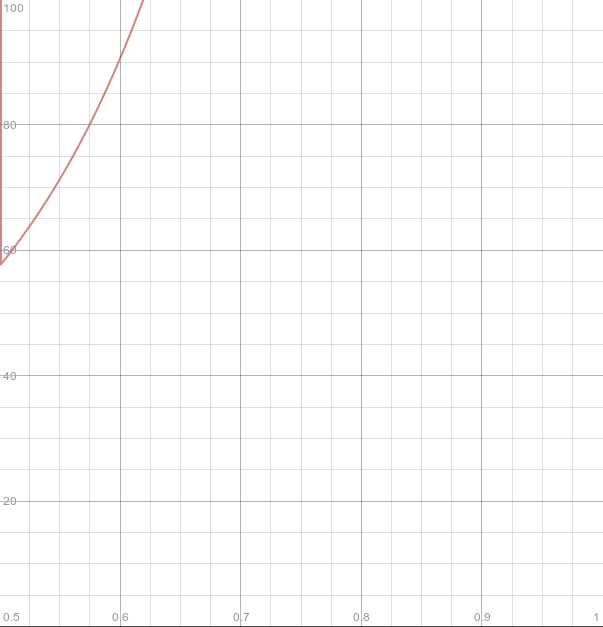
(a) $\epsilon=0.01$

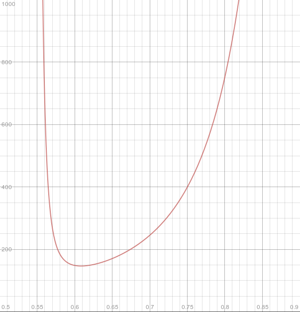
(b) $\epsilon=0.001$

Figure 1: Sample complexity vs. step-size parameter; $y:N^{\prime}_{0},x:k,\gamma=0.1$, $M$ = 1E-07

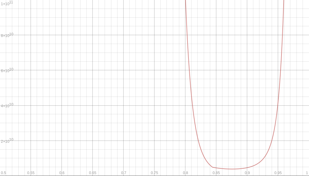
(a) $\epsilon=0.01$

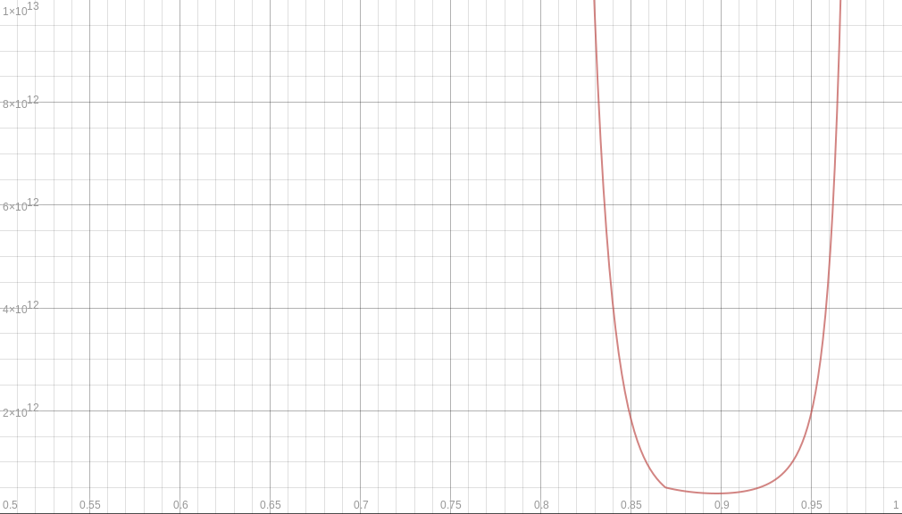
(b) $\epsilon=0.001$

Figure 2: Sample complexity vs. step-size parameter; $y:N^{\prime}_{0},x:k,\gamma=0.1$, $M$ = 100

From the graph it is clear that for large values of $M$, the optimal $k$ is biased towards $1$ whereas for small values of $k$ it is biased toward $\frac{1}{2}$. The reason is that for large $M$, with large step-size, $n_{0}$ will be much higher although $N^{\prime}_{0}-n_{0}$ is small whereas with very small $M$, even if we use large step-size, $n_{0}$ will not be large, thus one can take advantage of $N^{\prime}_{0}-n_{0}$ being small.

VII Conclusion

In this paper, we describe asymptotic and non-asymptotic convergence analysis of stochastic approximation recursions with Markov iterate-dependent noise using the lock-in probability framework. Our results show that we are able to recover the same bound available for lock-in probability in the literature for the much stronger i.i.d noise case. Such results are used to calculate sample complexity estimate of such stochastic approximation recursions which are then used for predicting the optimal step size. Moreover, our results are extremely useful to prove almost sure convergence to specific attractors in cases where asymptotic tightness of the iterates can be proved easily. An interesting future direction will be to extend this analysis to two-timescale scenarios with coupling both ways between the recursions and, both with and without Markov iterate-dependent noise.

Appendix A Proof of conditional and maximal version of Azuma’s inequality

Let $P_{B}$ denote probability measure defined by $P_{B}(A)=\frac{P(A\cap B)}{P(B)}$ where $B\in\mathcal{F}_{1}$. If we can show that with this new probability measure $\{S_{n}\}$ is a martingale, then we can follow the steps in [26, (3.30), p 227] to conclude the proof.

Let us denote by $E_{B}$ the expectation with respect to $P_{B}$. Clearly, $E_{B}(X)=\frac{\int_{B}XdP}{P(B)}$. Let $G\in\mathcal{F}_{n}$. Now,

$$\int_{G}E_{B}[S_{n+1}| \mathcal{F}_{n}]dP_{B}=E_{B}[E_{B}[I_{G}S_{n+1}|\mathcal{F}_{n}]]$$

$$=E_{B}[I_{G}S_{n+1}]=\frac{E[I_{G\cap B}S_{n+1}]}{P(B)}$$

$$=\frac{E[I_{G\cap B}E[S_{n+1}|\mathcal{F}_{n}]]}{P(B)}$$

$$=\frac{E[I_{G\cap B}S_{n}]}{P(B)}=\int_{G}S_{n}dP_{B}.$$

Appendix B General discrete Gronwall inequality

Let $\{\theta_{n},n\geq 0\}$ (respectively $\{a_{n},n\geq 0\})$ be non-negative (respectively positive) sequences, $L\geq 0$ and $f(n)$ be a increasing function of $n$ such that for all $n$

$$\theta_{n+1}\leq f(n)+L(\sum_{m=0}^{n}a_{m}\theta_{m}).$$

Then for $T_{n}=\sum_{m=0}^{n}a_{m}$,

$$\theta_{n+1}\leq f(n)e^{LT_{n}}$$

Proof.

Similar to the proof of Lemma 8 in Appendix B of [5] ∎

Prasenjit Karmakar received the Master’s and Ph.D. degrees in computer science and automation from the Indian Institute of Science in 20012 and 2018, respectively. He will soon join as a postdoctoral researcher at EE Technion. His research interests are in reinforcement learning, stochastic approximation and applied probability.

Shalabh Bhatnagar received the Bachelor’s (Hons.) degree in physics from the University of Delhi, Delhi, India, in 1988 and the Master’s and Ph.D. degrees in electrical engineering from the Indian Institute of Science, Bangalore, in 1992 and 1997, respectively. He is a Professor and Chairman with the Department of Computer Science and Automation as well as Robert Bosch Centre for Cyber Physical Systems, Indian Institute of Science, Bangalore. His research interests are in stochastic approximation theory and stochastic optimization and control, as well as applications in communication, wireless, and vehicular traffic networks.

References

• [1] M.Metivier and P.Priouret, β€œApplications of a Kushner-Clark lemma to general classes of stochastic algorithms,” IEEE Transactions on Information Theory, vol.Β 30, pp.Β 140–151, 1984.
• [2] A.Benveniste, M.Metivier, and P.Priouret, Adaptive Algorithms and Stochastic Approximation. Berlin - New York: Springer Verlag, 1990.
• [3] H.J.Kushner and G.Yin, Stochastic Approximation and Recursive Algorithms and Applications. New York: Springer, 2ndΒ ed., 2003.
• [4] C.Andrieu, V.B.Tadic, and M.Vihola, β€œOn the stability of some controlled Markov chains and its applications to stochastic approximation with Markovian dynamic,” Annals of Applied Probability, vol.Β 25, no.Β 1, pp.Β 1–45, 2015.
• [5] V.S.Borkar, Stochastic Approximation : A Dynamic Systems Viewpoint. Cambridge University Press, 2008.
• [6] C.Andrieu, E.Moulines, and P.Priouret, β€œStability of stochastic approximation under verifiable conditions,” SIAM Journal on Control and Optimization, vol.Β 44, no.Β 1, pp.Β 283–312.
• [7] H.F.Chen, β€œStochastic approximation and its applications,” SIAM Journal on Control and Optimization, vol.Β 44, pp.Β 283–312, July 2016.
• [8] V.S.Borkar, β€œOn the lock-in probability of stochastic approximation,” Combinatorics, Probability and Computing, vol.Β 11, pp.Β 11–20, 2002.
• [9] V.S.Borkar and S.Β Meyn, β€œThe o.d.e. method for convergence of stochastic approximation and reinforcement learning,” SIAM Journal on Control and Optimization, vol.Β 38, no.Β 2, pp.Β 447–469, 2000.
• [10] S.Kamal, β€œOn the convergence, lock-In probability, and sample complexity of stochastic approximation,” SIAM Journal on Control and Optimization, vol.Β 48, pp.Β 5178–5192, 2010.
• [11] V.R.Konda and J.N.Tsitsiklis, β€œLinear stochastic approximation driven by slowly varying Markov chains,” Systems and Control Letters, vol.Β 50, pp.Β 95–102, 2003.
• [12] G.Dalal, B.Szorenyi, G.Thoppe, and S.Mannor, β€œFinite sample analysis of two-timescale stochastic approximation with applications to reinforcement learning,” Conference on Learning Theory (COLT), 2018.
• [13] W.B.Arthur, Increasing Returns and Path Dependence in the Economy. University of Michigan Press, 1994.
• [14] O.Brandiere, β€œSome pathological traps for stochastic approximation,” SIAM Journal on Control and Optimization, vol.Β 36, no.Β 4, pp.Β 1293–1314, 1998.
• [15] R.Permantle, β€œNonconvergence to unstable points in urn models and stochastic approximations,” Annals of Probability, vol.Β 18, pp.Β 698–712, 1990.
• [16] G.Thoppe and V.S.Borkar, β€œA concentration bound for stochastic approximation via Alekseev’s formula,” Stochastic Systems(To Appear), 2018.
• [17] P.Karmakar and S.Bhatnagar, β€œTwo timescale stochastic approximation with controlled Markov noise and off-policy temporal difference learning,” Mathematics of Operations Research, vol.Β 43, no.Β 1, pp.Β 130–151, 2018.
• [18] M.Broadie, D.Cicek, and A.Zeevi, β€œGeneral Bounds and Finite-Time Improvement for the Kiefer-Wolfowitz Stochastic Approximation Algorithm,” Operations Research, vol.Β 59, no.Β 5, pp.Β 1211–1224, 2010.
• [19] A.Rakhlin, O.Shamir, and K.Sridharan, Making Stochastic Gradient Descent Optimal for Strongly Convex Problems. ICML, 2012.
• [20] L.Rosasco and T.Poggio, β€œConsistency, Learnability, and Regularization,” Lecture Notes for MIT Course 9.520, 2015.
• [21] R.Durrett, Probability Theory and Examples. Cambridge University Press, 4thΒ ed., 2010.
• [22] A.Ramaswamy and S.Bhatnagar, β€œStability of Stochastic Approximations with β€˜Controlled Markov’ Noise and Temporal Difference Learning,” IEEE Transactions on Automatic Control, 2018.
• [23] V.Yaji and S.Bhatnagar, β€œAnalysis of stochastic approximation schemes with set-val ued maps in the absence of a stability guarantee and their stabilization,” https://arxiv.org/abs/1701.07590, 2018.
• [24] V.S.Borkar and S.Pattathil, β€œConcentration bounds for two time scale stochastic approximation,” tech. rep., 2018.
• [25] A.Nemirovski, A.Juditsky, G.Lan, and A.Shapiro, β€œRobusT Stochastic Approximation Approach to Stochastic Programming,” SIAM Journal on Optimization, vol.Β 19, no.Β 4, pp.Β 1574–1609, 2009.
• [26] M.Habib, C.McDiarmid, J.Ramirez-Alfonsin, and B.Reed, ’Concentration’, in Probabilistic Methods for Algorithmic Discrete Mathematics. Berlin-Heidelberg: Springer Verla, 1998.