Probing the wind launching regions of the Herbig Be star HD 58647 with high spectral resolution interferometry

Abstract

We present a study of the wind launching region of the Herbig Be star HD 58647 using high angular ($\lambda/2B=0^{\prime\prime}.003$) and high spectral ($R=12000$) resolution interferometric VLTI-AMBER observations of the near-infrared hydrogen emission line, Br$\gamma$. The star displays double peaks in both Br$\gamma$ line profile and wavelength-dependent visibilities. The wavelength-dependent differential phases show S-shaped variations around the line centre. The visibility level increases in the line (by $\sim 0.1$) at the longest projected baseline (88 m), indicating that the size of the line emission region is smaller than the size of the K-band continuum-emitting region, which is expected to arise near the dust sublimation radius of the accretion disc. The data have been analysed using radiative transfer models to probe the geometry, size and physical properties of the wind that is emitting Br$\gamma$. We find that a model with a small magnetosphere and a disc wind with its inner radius located just outside of the magnetosphere can well reproduce the observed Br$\gamma$ profile, wavelength-dependent visibilities, differential and closure phases, simultaneously. The mass-accretion and mass-loss rates adopted for the model are $\dot{M}_{\mathrm{a}}=3.5\times 10^{-7}$ and $\dot{M}_{\mathrm{dw}}=4.5\times 10^{-8}\,\mathrm{M_{\sun}\,yr^{-1}}$, respectively ($\dot{M}_{\mathrm{dw}}/\dot{M}_{\mathrm{a}}=0.13$). Consequently, about 60 per cent of the angular momentum loss rate required for a steady accretion with the measured accretion rate is provide by the disc wind. The small magnetosphere in HD 58647 does not contribute to the Br$\gamma$ line emission significantly.

1 Introduction

Table 1: Summary of known properties of HD 58647.

$M_{*}$	$R_{*}$	$L_{*}$	Sp. Type	Age	$T_{\mathrm{eff}}$	$v\sin i$	$\dot{M_{a}}$	d	K	H	Av
($\mathrm{M_{\sun}}$)	($\mathrm{R_{\sun}}$)	($\mathrm{L_{\sun}}$)	…	(Myr)	($10^{3}$K)	(km s-1)	($\mathrm{M_{\sun}\,yr^{-1}}$)	(pc)	…	…
$3.0^{a}$	2.8a	911.2b	B9 IVe,f	$0.4^{b}$	10.5b	118f	$3.5\times 10^{-7}\,{}^{a}$	$318_{-46}^{+65}\,{}^{i}$	$5.4^{k}$	$6.1^{k}$	$0.4^{e}$
$4.2^{c}$		302c		$0.16^{c}$	10.7c	280g	$1.4\times 10^{-5\,h}$	$280_{-50}^{+80}\,{}^{c,j}$			$0.5^{c}$
		$295^{d}$						$543^{b}$

^aBrittain et al. (2007), ^bMontesinos et al. (2009), ^cvan den Ancker et al. (1998), ^dMonnier et al. (2005), ^eMalfait et al. (1998), ^fMora et al. (2001), ^gGrady et al. (1996), ^hMendigutía et al. (2011), ⁱvan Leeuwen (2007), ^jPerryman et al. (1997), ^kCutri et al. (2003).

Strong outflows are commonly associated with the early stages of stellar evolution. They are likely responsible for transporting excess angular momentum away from the star-disc system and regulating the mass-accretion process and spin evolution of newly born stars (e.g. Hartmann & Stauffer 1989; Matt & Pudritz 2005; Bouvier et al. 2014). There are at least three possible types of outflows around young stellar objects: (1) a disc wind launched from the accretion disc (e.g. Blandford & Payne 1982; Ustyugova et al. 1995; Romanova et al. 1997; Ouyed & Pudritz 1997; Ustyugova et al. 1999; Königl & Pudritz 2000; Pudritz et al. 2007), (2) an X-wind or a conical wind launched near the disc-magnetosphere interaction region (e.g. Shu et al. 1994, 1995; Romanova et al. 2009) and (3) a stellar wind launched from open magnetic field lines anchored to the stellar surface (e.g. Decampli 1981; Hartmann & MacGregor 1982; Kwan & Tademaru 1988; Hirose et al. 1997; Strafella et al. 1998; Romanova et al. 2005; Matt & Pudritz 2005; Cranmer 2009). However, despite recent efforts, the exact launching mechanisms of the winds and outflows as well as the mechanism behind the collimation of the ejected gas into jets are still not well understood (e.g. Edwards et al. 2006; Ferreira, Dougados, & Cabrit 2006; Kwan, Edwards, & Fischer 2007; Tatulli et al. 2007a; Kraus et al. 2008; Eisner, Hillenbrand, & Stone 2014). Hence, high-resolution interferometric observations which can resolve the wind launching regions are crucial for addressing this issue. If a high spectral resolution is combined with a high spatial resolution, the emission-line regions near the base of the wind (e.g., Br$\gamma$ emission regions in Herbig Ae/Be stars) can be resolved in many spectral channels across the line (e.g. Weigelt et al. 2011; Kraus et al. 2012a, b; Garcia Lopez et al. 2015). This allows us to study the wavelength-dependent extent and the kinematics of the winds, which can be derived from the line visibilities and wavelength-dependent differential and closure phases. Such observations would help us to distinguish the different types of outflow scenarios.

HD 58647 is a bright (K=5.4, H=6.1) Herbig Be star (B9 IV: The, de Winter, & Perez 1994; Malfait, Bogaert, & Waelkens 1998; Mora et al. 2001) which is located at 318 pc (van Leeuwen 2007; hereafter VL07). The star exhibits double-peaked profiles in some hydrogen emission lines, such as H$\alpha$ and Br$\gamma$ (e.g. Grady et al. 1996; Oudmaijer & Drew 1999; Harrington & Kuhn 2009; Brittain et al. 2007). The star does not show a significant variability in H$\alpha$ on time scales of 3 d (Mendigutía et al. 2011) and 1 yr (Harrington & Kuhn 2009). A presence of an intrinsic linear polarization in H$\alpha$ is reported in Vink et al. (2002), Mottram et al. (2007) and Harrington & Kuhn (2009). A relatively strong double-peaked Br$\gamma$ is reported in Brittain et al. (2007); however, no variability study is found for this line in the literature. The age of the star has been estimated as 0.4 Myr (van den Ancker, de Winter, & Tjin A Djie 1998) and 0.16 Myr (Montesinos et al. 2009), but some have also reported the possibilities of the star being an older classical Be star (e.g. Manoj, Maheswar, & Bhatt 2002; Berthoud et al. 2007). Using the broad K-band (2.18 $\micron$, $\Delta\lambda=0.3\,\micron$) Keck interferometer and a uniform ring geometric model, Monnier et al. (2005) (hereafter MO05) estimated the ring radius of the K-band continuum emission of HD 58647 as 0.82($\pm 0.13$) au, assuming the distance to the star is 280 pc (van den Ancker et al. 1998; Perryman et al. 1997). However, this radius may be underestimated since the ring inclination effect is not included in their study. Some of the known properties of HD 58647 are summarised in Table 1.

Here, we present VLTI-AMBER observations of the Herbig Be star HD 58647 with the high spectral resolution mode (HR-K-2.172) to resolve its Br$\gamma$ emission spatially and spectrally ($\mathrm{R}\approx 12000$, $\Delta v\approx 25\,\mathrm{km\,s^{-1}}$). The velocity extent of the Br$\gamma$ line profile for the star is about $\pm 200\,\mathrm{km\,s^{-1}}$ (Brittain et al. 2007); hence, this resolution will provide us with more than 16 velocity components across the line, which is essential for studying wind kinematics in a subsequent radiative transfer modelling. So far, there are only a few Herbig stars which are observed with the VLTI-AMBER in the high spectral resolution mode: Z CMa (Be + FUor, Benisty et al. 2010), MWC 297 (B1.5 V, Weigelt et al. 2011), HD 163296 (A1 V, Garcia Lopez et al. 2015), HD 98922 (B9 V, Caratti o Garatti et al. 2015) and HD 100564 (B9 V, Mendigutía et al. 2015). Kraus et al. (2012b) and Ellerbroek et al. (2015) have presented high spectral resolution VLTI-AMBER observations of V921 Sco (B[e]) and HD 50138 (B[e]), respectively, but their evolutionary states are not well known. These studies have successfully demonstrated the feasibility and usefulness of this type of observation for probing the kinematics and origin of the wind from Herbig stars. One notable difference between HD 58647 and other objects (MWC 297, HD 163296 and HD 98922) is the shape of Br$\gamma$. The former has a double-peaked and the latter have a single-peaked shaped line profile. It is interesting to study whether the difference is caused simply by the inclination angle effect or due to a fundamental difference in their wind structures. For example, the Br$\gamma$ emission could originate from a bipolar/stellar wind or a disc wind (e.g. Malbet et al. 2007; Tatulli et al. 2007a; Kraus et al. 2008; Eisner et al. 2010; Weigelt et al. 2011). If the line is double-peaked, the emission is most likely from a disc wind, which is rotating near Keplerian velocity at the base of the wind. If the line is single-peaked, it is likely formed in either a bipolar/stellar wind viewed at a mid to high inclination angle or a disc wind viewed at a low inclination angle (e.g. Kurosawa et al. 2006).

The interferometric data will be analysed by using the radiative transfer code torus (e.g., Harries 2000; Symington, Harries, & Kurosawa 2005; Kurosawa, Harries, & Symington 2006; Kurosawa, Romanova, & Harries 2011, hereafter KU11; Haworth & Harries 2012), which calculates hydrogen emission line profiles and line intensity maps using various inflow/outflow models of young stars. The code has been used to study classical T Tauri stars (Kurosawa, Harries, & Symington 2005; Kurosawa, Romanova, & Harries 2008; Kurosawa & Romanova 2012; Alencar et al. 2012; Kurosawa & Romanova 2013), a pre-FUor (Petrov et al. 2014) and a Herbig Ae star (Garcia Lopez et al. 2016) in the past. Based on the simulated emission maps computed in many velocity bins, we can reconstruct not only the line profiles, but also important interferometric quantities such as visibility, differential and closure phases across the line, which can be directly compared with the observations. To differentiate various possible outflow scenarios (e.g., a stellar wind and a disc wind), we will perform qualitative analysis of wind structures around YSOs by detailed radiative transfer models for the high resolution spectro-interferometric observations.

The aim of this paper is to investigate the nature and the origin of the wind around the Herbig Be star HD 58647 by means of high spectral resolution interferometric observations combined with radiative transfer modellings. In Section 2, we describe our VLTI-AMBER observations and data reduction. A simple geometrical model to characterise the size of continuum emission is presented in Section 3. The description of the radiative transfer models and the results of model fits to the observations are given in Section 4. Brief discussions on our results are given in Section 5. Finally, the summary of our findings and conclusions are presented in Section 6.

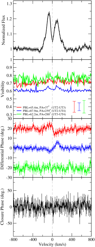
Figure 1: Summary of the high-spectral-resolution AMBER observations around Br$\gamma$ using three baselines. The figure shows the average normalised flux around Br$\gamma$ from 3 telescopes (top panel), the visibilities (second panel from the top), differential phases (third panel from the top) and closure phases (bottom panel) as a function of velocity. For clarity, the differential phases for the first (red) and third (green) baselines are shifted vertically by $+20^{\circ}$ and $-20^{\circ}$, respectively. Thin vertical lines indicate the uncertainty in each data point. In the visibility plot (the second panel from the top), the typical uncertainty levels are indicated on the lower-right corner.

Table 2: Log for high-spectral-resolution VLTI-AMBER observation of HD 58647 using the telescope configuration UT2-UT3-UT4.

Object	Type	Date	Time [UT]	Mode	$\lambda$ Range	DITa	NDITb	Seeing
					($\micron$)	(s)		(”)
HD 58647	Target	2015-01-02	04:31 – 05:13	HR-K-F	2.147–2.194	0.75	2400	0.75 – 1.0
HD 57939	Calibrator	2015-01-02	05:24 – 05:35	HR-K-F	2.147–2.194	0.75	600	0.87 – 1.1

^aDetector integration time per interferogram. ^bTotal number of interferograms.

Table 3: Log for low-spectral-resolution VILT-AMBER observations of HD 58647.

Data set	UT date	UT time	DIT	NDIT	Telescopes	Proj. baselines	PA	ESO Prog. ID
	(yyyy:mm:dd)	(hh:mm)	(s)		(ATs)	(m)	(∘)
A	2009-11-11	08:24	0.05	5000	D0-K0-H0	63.5/31.7/95.2	70.2/70.1/70.2	084.C-0170
B	2009-11-11	09:07	0.05	2000	D0-K0-H0	64.0/32.0/95.9	72.8/72.8/72.8	084.C-0170
C	2009-11-12	08:00	0.05	2500	D0-G1-H0	71.5/62.5/70.2	131.2/68.5/3.5	084.C-0170
D	2009-11-12	08:22	0.05	1500	D0-G1-H0	71.3/63.5/70.3	131.7/70.2/5.9	084.C-0170
E	2010-12-31	03:07	0.05	5000	I1-H0-G0	26.6/40.1/50.5	57.5/141.0/109.5	086.C-0267
F	2010-12-31	03:41	0.05	5000	I1-H0-G0	28.6/40.6/53.5	62.0/142.2/110.4	086.C-0267
G	2011-02-12	01:59	0.10	5000	I1-H0-G1	40.7/45.3/70.2	146.2/37.0/3.8	086.C-0267

2 Observations and data reductions

The Herbig Be star HD58647 (B9 IV) was observed during the second half of the night of January 1, 2015 using the Very Large Telescope Interferometer (VLTI) with the AMBER beam combiner instrument (Petrov et al. 2007), as a part of the observing programme 094.C-0164 (PI: Kurosawa). The combination of UT2-UT3-UT4 telescopes along with the high spectral resolution mode (R=12000) of AMBER were used. The log of the observations is summarised in Table 2. The interferograms were obtained using the fringe tracker FINITO for co-phasing with the detector integration time (DIT) of 0.75 s for each interferogram. The total of 2400 interferograms were recorded, or equivalently about 30 min of total integration time was used. In addition to our target, HD 57939 (K0 III) was observed with the same DIT, as an interferometric calibrator.

The fringe tracking performance typically varies between the target and calibrator observations; therefore, low-resolution (LR, R $\approx$ 35) AMBER observations (ESO Prog. ID: 084.C-0170 and 086.C-0267, PI: Natta) are used to calibrate the continuum visibilities. A summary of the LR observations is shown in Table 3. The data were reduced with the AMBER data processing software amdlib (v3.0.5) (Tatulli et al. 2007b; Chelli, Utrera, & Duvert 2009), which is available at http://www.jmmc.fr/data_processing_amber.htm. Furthermore, for the reduction of the LR data, we applied a software that equalizes the optical path difference (OPD) histograms of the object and calibrator (Kreplin et al. 2012). The end products of the data reduction process are the wavelength-dependent normalised flux (averaged over 3 telescopes), visibilities, differential phases, and closure phases. The typical errors in the observed visibilities are approximately 5 to 9 per cent. The results are summarised in Fig. 1.

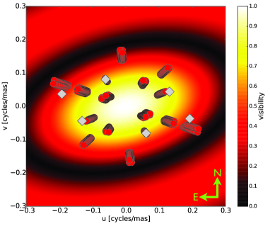
Figure 2: The $uv$ points used for the low-spectral-resolution (filled circle, Tabel 3) and high-spectral-resolution (filled diamond, Tabel 2) AMBER observations are overplotted with the visibility from a geometrical ring model. The parameters used for the ring model are summarised in Table 4. The position angles of the baselines are measured from north to east. Here,  $u$ decreases towards east which is the opposite to the sense used in the usual convention (e.g. Thompson, Moran, & Swenson, Jr. 2001).

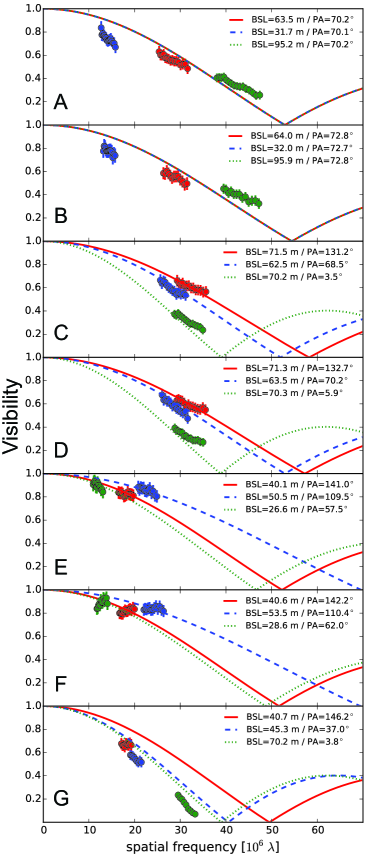
Figure 3: Summary of a geometrical ring model fit for the circumstellar visibilities ($V_{\mathrm{circ}}$) from the low-resolution (LR, $R\approx 35$) VLTI-AMBER observations (Table 3). The circumstellar visibilities from 7 different sets of measurements (Sets A–G in Table 3 from top to bottom) are shown as a function of spatial frequency (small circles with error bars). The dashed, dotted and solid lines are the model visibility curves of the two-dimensional (elongated ring) model at the same PAs as in the observations. The corresponding parameters used in the best-fit model are summarised in Table 4. The corresponding $uv$ coverage of the LR VLTI-AMBER observations are shown in Fig. 2. Note that all the model visibility curves nearly overlap in the top two panels, thus they are hard to distinguish from the others.

The figure clearly shows that Br$\gamma$ is double peaked with its peaks at around 25 per cent above the continuum. The dip is located at the line centre. The double-peaked line profiles are likely caused by the rotation of the gas around the star, most likely in a disc wind (e.g. Shlosman & Vitello 1993; Knigge et al. 1995; Sim et al. 2005; Kurosawa et al. 2006). This will be further investigated in Section 4. The wavelength-dependent visibilities are rather noisy, but those from the longest projected baseline (87.9 m) clearly show that the visibility level increases in the line. The visibility curve also shows a double-peak appearance. The noise levels in the visibility curves from the shorter baselines (45.4 and 62.2 m) are somewhat higher; therefore, the double-peak feature is only weakly suggested. The increases of the visibilities in the emission line with respect to those in the continuum indicate that the size of line-emitting region is smaller than that of the K-band continuum-emitting region.

The wavelength-dependent differential phases show S-shape curves around the line centre for two projected baselines (45.4 and 87.9 m). In both cases, the differential phase crosses 0 near the line centre. The sense of the S-shape pattern is opposite between the two. The deviation of the differential phases from $0^{\circ}$ indicates a shift in the photocentre at the velocity channel. Since the pattern of the differential phase curves is sensitive to the kinematics and geometry of the line-emitting gas, this will be used to constrain the gas outflow models used in the radiative transfer calculations which are to be presented later in Section 4.3. Lastly, the wavelength-dependent closure phases do not show any significant deviation from $0^{\circ}$ within the range of uncertainties which are typically around $\pm 20^{\circ}$.

Table 4: Parameters of the best-fit geometrical ring model for the low-resolution AMBER visibilities.

Model	$R_{\mathrm{ring}}$	$i$	PA
	(mas)	(∘)	(∘)
Ring	$2.0(\pm 0.3)$	$55(\pm 2)$	$105(\pm 4)$

3 A simple geometrical model for the continuum emission region

To estimate the characteristic size of the K-band continuum emission of HD 58647, we fit the observed visibilities of the LR VLTI-AMBER observations, listed in Table 3, with a simple geometrical ring model. Since the observed visibilities ($V_{\mathrm{obs}}$) are influenced by both unresolved stellar flux ($F_{*}$) and that from the circumstellar matter ($F_{\mathrm{circ}}$), we first calculate the circumstellar visibilities ($V_{\mathrm{circ}}$) as follows:

$$V_{\mathrm{circ}}=\frac{\left|V_{\mathrm{obs}}\left(F_{*}+F_{\mathrm{circ}}\right)-F_{*}V_{*}\right|}{F_{\mathrm{circ}}}$$ (1)

where $V_{*}$ is the stellar visibility (e.g. Kreplin et al. 2012). Here, we assume $V_{*}=1$ since the central star is unresolved (its angular radius is $\sim$0.07 mas at the distance of 318 pc, VL07). To estimate the ratio of the circumstellar to stellar fluxes, we compare the stellar atmosphere model of Kurucz (1979) with $T_{\mathrm{eff}}=10500\,$K and $\log g_{*}=3.5$ (Montesinos et al. 2009) with the K-band photometry data from VO SED Analyzer tool (VOSA, Bayo et al. 2008), after dereddening the data ($A_{V}=0.4$ , Malfait et al. 1998). The original photometric data are from Ochsenbein, Bauer, & Marcout (2000). The target distance ($d\sim 318$ pc, VL07) is adopted from the Hipparcos measurement. We find the flux ratio is $F_{\mathrm{circ}}/F_{*}=2.9$ at $\mbox{$\lambda$=}2.2\,\micron$. Using this value and equation 1, the circumstellar visibilities $V_{\mathrm{circ}}$ are determined for each set of the LR VLTI-AMBER observations (Table 3). The results are shown in Fig. 3. The figure suggests that the emission geometry deviates from a spherical symmetry because e.g. the circumstellar visibilities at the spatial frequency $\sim 30\times 10^{6}\,\lambda$ (e.g. in the data sets C and D) are notably different for the baselines with different position angles.

To model the circumstellar visibilities $V_{\mathrm{circ}}$, we consider an inclined uniform ring geometry with an inner radius $R_{\mathrm{ring}}$ and a width $\Delta R_{\mathrm{ring}}$ because the K-band continuum of the discs of Herbig stars is expected to originate mainly from the region near the dust sublimation radius (e.g. MO05; Dullemond & Monnier 2010). Here, we assume $\Delta R_{\mathrm{ring}}=0.2\,R_{\mathrm{ring}}$ as in MO05. The elongation of the ring occurs when the circular ring has an inclination angle $i>0^{\circ}$. We use this two-dimensional model to fit the set of all visibilities from the LR observations simultaneously, instead of fitting one-dimensional model visibilities to individual observed visibilities. The results of the best-fit model are shown in Fig. 3. The corresponding model parameters are summarised in Table 4. As one can see from the figure, the simple geometrical model with a ring can reasonably fit the observed visibilities. In this analysis, we find that the angular radius of the K-band continuum-emitting ring is around 2.0 mas (Table 4), which corresponds to 0.64 au at the distance of 318 pc (VL07).

4 Radiative Transfer Models

To model the interferometric quantities obtained by VLTI-AMBER in the high-spectral-resolution mode, i.e. the wavelength-dependent flux, visibility and differential and closure phases around Br$\gamma$ presented in Section 2, we use the radiative transfer code torus (e.g. Harries 2000; Symington et al. 2005; Kurosawa et al. 2006; KU11). The numerical method used in the current work is essentially the same as in KU11. The model uses the tree-structured grid (octree/quadtree in 3-D and 2-D, respectively) in cartesian coordinate, but here we assume axisymmetry around the stellar rotation axis. The atomic model consists of hydrogen with 20 energy levels, and the non-local thermodynamic equilibrium (non-LTE) level populations are solved using the Sobolev approximation (e.g. Sobolev, 1957; Castor, 1970; Castor & Lamers, 1979). More comprehensive descriptions of the code are given in KU11.

For the present work, we have made three minor modifications to the code in KU11: (1) the model now includes the continuum emission from a geometrically flat ring which simulates the K-band dust emission near the dust sublimation radius, (2) the effect of rotation of a magnetosphere has been included by using the method described in Muzerolle, Calvet, & Hartmann (2001), and (3) the code has been modified to write model intensity maps as a function of wavelength (or velocity bins). The first modification is important for modelling a correct line strength of Br$\gamma$ (2.2166 $\mu$m) and the interferometric quantities around the line. The second modification is included because intermediate-mass Herbig Ae/Be stars are expected to be rotating relatively fast with their rotation periods about $0.2$ to a few days (e.g. Hubrig et al. 2009, but see also Hubrig et al. 2011). Until now, our model has been applied mainly to classical T Tauri stars which rotate relatively slowly with their rotation period 2–10 d (e.g. Herbst et al. 1987; Herbst et al. 1994) in which the effect of rotation is rather small (e.g. Muzerolle et al. 2001). The third modification is important because it will allow us to compute the interferometric quantities, such as visibility, differential and closure phases, as a function of wavelength. This enables us to directly compare our models with the spectro-interferometric data from VLTI-AMBER.

4.1 Model configurations

There are 4 distinct emission components in our model: (1) the central star, (2) the magnetospheric accretion funnels as described by Hartmann, Hewett, & Calvet (1994) and Muzerolle et al. (2001), (3) the disc wind which emerges from the equatorial plane (a geometrically thin accretion disc) located outside of the magnetosphere and (4) the geometrically flat ring which simulates the K-band dust emission near the dust sublimation radius. A basic schematic diagram of our models is shown in Fig. 4. In the following, we briefly describe each component and the key parameters. More comprehensive descriptions of the magnetosphere and disc wind components can be found in KU11.

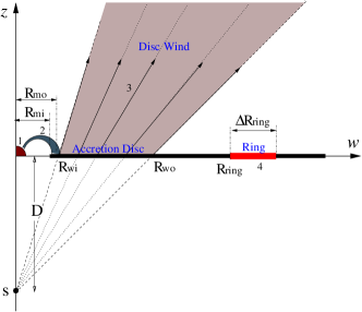
Figure 4: The model configuration of the circumstellar materials around the Herbig Be star HD 58647. The density is assumed to be axisymmetric and top-down symmetric. The model consists of: (1) the stellar continuum source (star) located at the origin of the cartesian coordinates system ($w$,$z$), (2) the magnetospheric accretion flow, (3) the disc wind, (4) the K-band continuum-emitting ring, and (5) the geometrically thin accretion disc. The split-monopole (with the source displacement distance $D$) disc wind emerges from the equatorial plane, but only within the distances from $z$-axis between $R_{\mathrm{wi}}$ and $R_{\mathrm{wo}}$. The geometrically thin ring with its inner radius $R_{\mathrm{ring}}$ and width $\Delta R_{\mathrm{ring}}$ is also placed on the equatorial plane. See Section 4.1 for more information. The figure is not to scale.

4.1.1 Central star

The central star is the main source of continuum radiation which ionizes the gas in the flow components (a magnetospheric accretion and a disc wind). For a given effective temperature $T_{\mathrm{eff}}$ and its surface gravity $\log g_{*}$, we use the stellar atmosphere model of Kurucz (1979) as the photospheric contribution to the continuum in our model. Our underlying central star is a late B-type star; hence, the photospheric absorption component from the star may affect the shape of the model Br$\gamma$ profiles. For this reason, we use the high-spectral-resolution synthetic phoenix (Hauschildt & Baron 1999) spectra from Husser et al. (2013), convolved with $v\sin i=118\,\mathrm{km~{}s^{-1}}$ (Mora et al. 2001) for the photospheric absorption profile for Br$\gamma$.

4.1.2 Magnetosphere

We adopt a dipole magnetic field geometry with its accretion stream described by $r=R_{\mathrm{m}}\,\sin^{2}{\theta}$ where $r$ and $\theta$ are the polar coordinates; $R_{\mathrm{m}}$ is the magnetospheric radius on the equatorial plane, as in e.g. Ghosh et al. (1977) and Hartmann et al. (1994). In this model, the accretion occurs in the funnel regions defined by two stream lines which correspond to the inner and outer magnetospheric radii, i.e., $R_{\mathrm{m}}=R_{\mathrm{mi}}$ and $R_{\mathrm{mo}}$ (Fig. 4). As in KU11, we follow the density and temperature structures along the stream lines as in  Hartmann et al. (1994) and Muzerolle et al. (2001). The temperature scale is normalised with a parameter $T_{\mathrm{m}}$ which sets the maximum temperature in the stream. The mass-accretion rate $\dot{M}_{\mathrm{a}}$ scales the density of the magnetospheric accretion funnels. We adopt the method described in Muzerolle et al. (2001) (their Appendix A), to include the effect of rotation in the accretion funnels.

4.1.3 Disc wind

As in KU11, the disc wind model used here is based on the ‘split-monopole’ wind model by e.g. Knigge et al. (1995) and Long & Knigge (2002) (see also Shlosman & Vitello 1993). The outflow arises from the surface of the rotating accretion disc, and has a bi-conical geometry. Most influential parameters in our models are: (1) the total mass-loss rate in the disc wind ($\dot{M}_{\mathrm{dw}}$), (2) the degree of the wind collimation, (3) the steepness of the radial velocity ($\beta_{\mathrm{dw}}$ in equation 2 below), and (4) the wind temperature. Fig. 4 shows the basic configuration of the disc-wind model. The wind arises from the disc surface. The wind “source” points ($S$), from which the stream lines diverge, are placed at distance $D$ above and below the centre of the star. The angle of the wind launching is controlled by changing the value of $D$. The wind launching is confined between $R_{\mathrm{wi}}$ and $R_{\mathrm{wo}}$ where the former is normally set to the outer radius of the closed magnetosphere ($R_{\mathrm{mo}}$) and the latter to be a free parameter. The wind density is normalised with the total mass-loss rate in the disc wind ($\dot{M}_{\mathrm{dw}}$) while the local mass-loss rate per unit area ($\dot{m}$) follows the power-law $\dot{m}\propto w^{-p}$ where $w$ is the distance from the star on the equatorial plane and $p=2.4$ (our fiducial value which produces reasonable Br$\gamma$ line profiles).

The poloidal component of the wind velocity ($v_{\mathrm{p}}$) is parametrised as:

$$v_{\mathrm{p}}\left(w_{i},l\right)=c_{\mathrm{s}}\left(w_{i}\right)+\left[f\,v_{\mathrm{esc}}-c_{\mathrm{s}}\left(w_{i}\right)\right]\left(1-\frac{R_{\mathrm{s}}}{l+R_{\mathrm{s}}}\right)^{\beta_{\mathrm{dw}}}$$ (2)

where $w_{i}$, $c_{\mathrm{s}}$, $f$, and $l$ are the distance from the rotational axis ($z$) to the wind emerging point on the disc, the sound speed at the wind launching point on the disc, the constant scale factor of the asymptotic terminal velocity to the local escape velocity ($v_{\mathrm{esc}}$ from the wind emerging point on the disc), and the distance from the disc surface along stream lines respectively. $R_{s}$ is the wind scale length, and is set to 10 $R_{\mathrm{wi}}$ by following Long & Knigge (2002). The azimuthal component of the wind velocity $v_{\phi}\left(w,z\right)$ is computed from the Keplerian rotational velocity at the emerging point of the stream line i.e. $v_{\phi}\left(w_{i},0\right)=\left(GM_{*}/w_{i}\right)^{1/2}$ by assuming the conservation of the specific angular momentum along a stream line, i.e. $v_{\phi}\left(w,z\right)\,=v_{\phi}\left(w_{i},0\right)\,\left(w_{i}/w\right)$.

The temperature of the wind ($T_{\mathrm{dw}}$) is assumed to be isothermal. This is a reasonable assumption because the studies of disc wind thermal structures by e.g. Safier (1993) and Garcia et al. (2001) have shown that the wind is heated by ambipolar diffusion, and its temperature reaches $\sim 10^{4}$ K quickly after being launched. Further, their studies have shown that the wind temperature remains almost constant or only slowly changes as the wind propagates after the temperature reaches $\sim 10^{4}$ K.

4.1.4 The K-band continuum-emitting ring

Since the K-band continuum of the accretion discs of Herbig stars is expected to originate mainly from the region near the dust sublimation radius (e.g. Dullemond & Monnier 2010), we simulate this emission with a geometrically thin ring on the equatorial plane, with its inner radius $R_{\mathrm{ring}}$ and its width $\Delta R_{\mathrm{ring}}$ (Fig. 4). This is the same geometrical model used to fit the continuum visibilities in Section 3. Again, we assume $\Delta R_{\mathrm{ring}}=0.2\,R_{\mathrm{ring}}$, as in MO05. The ring is assumed to have a uniform temperature $T_{\mathrm{ring}}=1500\,\mathrm{K}$, and to radiate as a blackbody.

4.2 Modelling Br$\gamma$ line profiles

Since computing the wavelength/velocity-dependent image maps is rather computationally expensive, we first concentrate on modelling the Br$\gamma$ profile (top panel in Fig. 1) obtained with the AMBER instrument to find a reasonable set of model parameters which approximately matches the observed line profile. Then, we will expand the model constraints to the rest of the observed interferometric quantities (visibilities, differential and closure phases) to further refine the model fit by computing the wavelength/velocity-dependent image maps for each model (Section 4.3).

4.2.1 Adopted stellar parameters

The basic stellar parameters adopted for modelling the observed AMBER data of our target HD 58647 are summarised in Table 5. We estimated the stellar luminosity $L_{*}$ by fitting the SED of HD 58647 using the VOSA online SED analyzing tool (Bayo et al. 2008) using $T_{\mathrm{eff}}=10500$ K and $\log g_{*}=3.5$ (cgs) (Montesinos et al. 2009), the extinction $A_{V}=0.4$ (Malfait et al. 1998) and the distance $d=318$ pc (VL07). From this fit, we find $L_{*}=412\,\mathrm{L_{\sun}}$. Using the evolutionary tracks of pre-main sequence stars by Siess, Dufour, & Forestini (2000) with the stellar luminosity found above and $\log g_{*}=3.5$, the stellar mass and radius of HD 58647 are estimated as $M_{*}=4.6\,\mathrm{M_{\sun}}$ and $R_{*}=6.2\,\mathrm{R_{\sun}}$, respectively.

The inclination angle $i$ of the K-band continuum-emitting ring was estimated as $i\approx 55^{\circ}$ in Section 3 (Table 4) by fitting the continuum visibilities. Assuming the disc/ring normal vector coincides with the rotation axis of HD 58647 and the speed at which the star rotates at the equator ($v_{\mathrm{eq}}$) is same as $v$ in $v\sin i$, we obtain $v_{\mathrm{eq}}=144\,\mathrm{km\,s^{-1}}$ (approximately $0.34$ of the breakup velocity) using $v\sin i=118\,\mathrm{km~{}s^{-1}}$ (Mora et al. 2001). Consequently, the rotation period of HD 58647 is estimated as $P_{*}=2\pi R_{*}/v_{\mathrm{eq}}=2.2$ d. We adopt the mass-accretion rate $\dot{M}_{\mathrm{a}}=3.5\times 10^{-7}\,\mathrm{M_{\sun}\,yr^{-1}}$ (Brittain et al. 2007), which is estimated from the CO line luminosity, in our magnetospheric accretion model.

Table 5: Adopted parameters of HD 58647 models.

$R_{*}$	$M_{*}$	$T_{\mathrm{eff}}$	$P_{*}$	$d$	$\dot{M}_{\mathrm{a}}$	$i$
($\mathrm{R_{\sun}}$)	($\mathrm{M_{\sun}}$)	($\mathrm{K}$)	(d)	($\mathrm{pc}$)	($\mathrm{M_{\sun}\,yr^{-1}}$)	(∘)
$6.2$	$4.6$	$10500$	$2.2$	$318$	$3.5\times 10^{-7}$	$55$

Table 6: Main model parameters.

	Magnetosphere				Disc wind							Continuum Ring
	$R_{\mathrm{mi}}$	$R_{\mathrm{mo}}$	$T_{\mathrm{m}}$		$\dot{M}_{\mathrm{dw}}$	$R_{\mathrm{wi}}$	$R_{\mathrm{wo}}$	$D$	$T_{\mathrm{dw}}$	$\beta_{\mathrm{dw}}$		$R_{\mathrm{ring}}$	$\Delta R_{\mathrm{ring}}$
Model	($R_{*}$)	($R_{*}$)	($\mathrm{K}$)		($\mathrm{M_{\sun}\,yr^{-1}}$)	($R_{*}$)	($R_{*}$)	($R_{*}$)	($\mathrm{K}$)	$\cdots$		($R_{*}$)	($R_{\mathrm{ring}}$)
A	$1.3$	$1.7$	$7500$		$\cdots$	$\cdots$	$\cdots$	$\cdots$	$\cdots$	$\cdots$		$\cdots$	$\cdots$
B	$1.3$	$1.7$	$8000$		$\cdots$	$\cdots$	$\cdots$	$\cdots$	$\cdots$	$\cdots$		$\cdots$	$\cdots$
C	$1.3$	$1.7$	$8500$		$\cdots$	$\cdots$	$\cdots$	$\cdots$	$\cdots$	$\cdots$		$\cdots$	$\cdots$
D	$1.3$	$1.7$	$8000$		$\cdots$	$\cdots$	$\cdots$	$\cdots$	$\cdots$	$\cdots$		$23.5$	$0.2$
E	$\cdots$	$\cdots$	$\cdots$		$4.5\times 10^{-8}$	$1.7$	$23.5$	$100$	$10^{4}$	$2.0$		$23.5$	$0.2$
F	$1.3$	$1.7$	$8000$		$4.5\times 10^{-8}$	$1.7$	$23.5$	$100$	$10^{4}$	$2.0$		$23.5$	$0.2$

4.2.2 Br$\gamma$ profiles from magnetospheric accretion models

Here, we briefly examine the effect of magnetospheric accretion (Section 4.1.2) on the formation of the hydrogen recombination line Br$\gamma$. Using the stellar parameters above, the corotation radius ($R_{\mathrm{cr}}$) of HD 58647 is estimated as $R_{\mathrm{cr}}=\left(GM_{*}\right)^{1/3}\left(P_{*}/2\pi\right)^{2/3}=1.9\,R_{*}$. The extent of the magnetosphere is assumed to be slightly smaller than $R_{\mathrm{cr}}$; hence, we set the inner and outer radii of the magnetospheric accretion funnel as $R_{\mathrm{mi}}=1.3\,R_{*}$ and $R_{\mathrm{mo}}=1.7\,R_{*}$, respectively. These radii (in units of the stellar radius) are considerably smaller than those of classical T Tauri stars (e.g. Königl 1991; Muzerolle et al. 2004) which typically has larger rotation periods, i.e. 7–10 d (e.g. Herbst et al. 2002). The smaller magnetosphere size in HD 58647 leads to smaller volumes for the accretion funnels. Hence, the hydrogen line emission is also expected to be much weaker. Muzerolle et al. (2004) also found that the emission lines from a small and rotating magnetosphere were very weak in their Balmer line models for the Herbig Ae star UX Ori (see their Fig. 3).

Fig. 5 shows a comparison of the observed Br$\gamma$ profile from the AMBER observation (Section 2) with the model profiles computed using the parameters for HD 58647 (Table 5). The models are computed for 3 different magnetospheric temperatures: $T_{\mathrm{m}}=7500$, 8000 and 8500 K (Models A, B and C in Table 6, respectively). The continuum emission from the ring are omitted here so that the emission component from the magnetosphere can be seen more easily. As expected, the lines are rather weak, and are mainly in absorption except for very small emission components around the velocities $v=\pm 100\,\mathrm{km~{}s^{-1}}$ in the lower temperature models (Models A and B). No significant emission above the continuum level is seen for models with $T_{\mathrm{m}}>8500\,\mathrm{K}$. Similar line shapes and strength are also found in the small magnetosphere model of Muzerolle et al. (2004) (their Fig. 3).

The models clearly disagree with the observed line profiles in their emission strengths, i.e. the emission from the magnetosphere is much weaker than the observed one. If the ring continuum emission is included in the models, the emission components in the models will appear even weaker. As suggested by Muzerolle et al. (2004), one way to increase the emission strength is to increase the size of magnetosphere; however, this will be in contradiction with the stellar parameters estimated earlier. It is most likely that an additional gas flow component is involved in the formation of the Br$\gamma$ emission line. This possibility will be explored next.

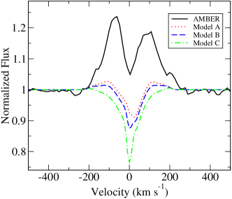
Figure 5: Comparison of the observed Br$\gamma$ line profile (solid) with the line profiles computed at the inclination angle $i=55^{\circ}$ with a rotating magnetosphere with different temperatures: $T_{\mathrm{m}}=$ 7500 (Model A, dot), 8000 (Model B, dash) and 8500 K (Model C, dash-dot). The models use the magnetosphere with $R_{\mathrm{mi}}=1.3\,\mathrm{R_{\sun}}$, $R_{\mathrm{mo}}=1.7\,\mathrm{R_{\sun}}$ and $\dot{M}_{\mathrm{a}}=3.5\times 10^{-7}\,\mathrm{M_{\sun}\,yr^{-1}}$ (Brittain et al. 2007). All the models show a rather strong central absorption component. Only the models with $T_{\mathrm{m}}<8000$ K show very weak emission components. For clarity, the continuum emission from the ring in the accretion disc and the photospheric absorption component are not included here.

Table 7: Ranges of the disc wind and continuum-emitting ring model parameters explored.

$\dot{M}_{\mathrm{dw}}$	$D$	$T_{\mathrm{dw}}$	$\beta_{\mathrm{dw}}$	$R_{\mathrm{ring}}$
($10^{-8}\,\mathrm{M_{\sun}\,yr^{-1}}$)	($R_{*}$)	($\mathrm{K}$)	$\cdots$	($R_{*}$)
3.0–6.0	50–200	9000–11000	1.5–2.5	21–27

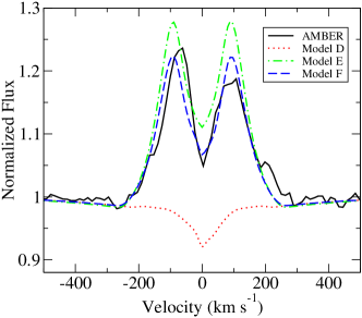
Figure 6: Comparison of the Br$\gamma$ line profiles computed with (1) a magnetosphere only (Model D, dotted), (2) a disc wind only (Model E, dash-dot) and (3) a magnetosphere and a disc wind (Model F, dash). The models are computed at $i=55^{\circ}$ and with the continuum-emitting ring and photospheric absorption component. The main model parameters used are summarised in Table 6. The Br$\gamma$ profile from the AMBER observation (solid) is also shown for a comparison. The line profile from the magnetosphere only model (Model D) is mainly in absorption, with relatively strong absorption near the line centre. The model with the magnetosphere and disc wind (Model F) fit the observation reasonably well. The central absorption dip is enhanced by the absorption in the magnetosphere, and the corresponding match with the observation is slightly better than the model with the disc wind alone (Model E).

4.2.3 Br$\gamma$ profiles from disc wind models

To bring the line strength of the model Br$\gamma$ to a level consistent with the one detected in the AMBER spectra, we now consider an additional flow component, namely the disc wind, as briefly described in Section 4.1.3. We have explored various combinations of the disc wind model parameters (i.e. $\dot{M}_{\mathrm{dw}}$, $D$, $T_{\mathrm{dw}}$ and $\beta_{\mathrm{dw}}$ as in Section 4.1.3; see also Fig. 4) and the continuum-emitting ring size ($R_{\mathrm{ring}}$ as in Section 4.1.4) to fit the observed Br$\gamma$ from the AMBER observation. The range of the model parameters explored are summarised in Table 7. In this analysis, we set the inner and outer wind radii ($R_{\mathrm{wi}}$ and $R_{\mathrm{wo}}$) to coincide with the outer radius of the magnetosphere $R_{\mathrm{mo}}$ and the ring radius ($R_{\mathrm{ring}}$), respectively. $R_{\mathrm{wi}}$ is set to the magnetospheric radius because a magnetosphere would set the inner radius of the accretion disc where the disc wind mass-loss flux would be highest (e.g. Krasnopolsky et al. 2003), and because a wind could arise in the disc-magnetosphere interaction region (e.g. Shu et al. 1994, 1995; Romanova et al. 2009). The outer wind launching radius $R_{\mathrm{wo}}$ is set to $R_{\mathrm{ring}}$ because the size of Br$\gamma$ emission was found to be smaller than the size of the K-band continuum-emitting region in Section 2, i.e. the visibility level increases in the line (by $\sim 0.1$) at the longest projected baseline of the VLTI-AMBER observation (Fig. 1). Hence, no significant wind emission is expected to be seen at radial distances beyond $R_{\mathrm{ring}}$.

Fig. 6 shows that our model with a magnetosphere plus disc wind (Model F) can reasonably reproduce the observed Br$\gamma$ profile. The figure also shows the models computed with a magnetosphere only (Model D) and a disc wind only (Model E) to demonstrate the contributions from each component. The corresponding model parameters are shown in Table 6. As one can see from the figure, the emission line is much stronger when the emission from the disc wind is included in the model. The match between the observation and Model F is quite good. As seen in the previous section, the line profile from the magnetosphere only model (Model D) is mainly in absorption, and the emission from the disc wind is dominating the line. The central absorption dip is enhanced by the absorption in the magnetosphere, and the corresponding match with the observation is slightly better for Model F, compared to the model with the disc wind alone (Model E). In Model F, the ratio of the mass-loss rate in the wind to the mass-accretion rate ($\mu=\dot{M}_{\mathrm{dw}}/\dot{M}_{\mathrm{a}}$) is about 0.13.

A prominent characteristics in the model profiles is their double-peaked appearance. Since these lines are mainly formed near the base of the disc wind where the Keplerian rotation of the wind is dominating over the poloidal motion, the double-peak profiles naturally occurs when the disc wind is viewed edge-on, i.e., when a system has a mid to high inclination angle ($i$). The extent of the line profile can be also explained by the Keplerian velocity ($V_{\mathrm{k}}$) of the disc. At the inner radius of the disc wind ($R_{\mathrm{wi}}=1.7\,R_{*}$), $V_{\mathrm{k}}=289\,\mathrm{km~{}s^{-1}}$. The corresponding projected velocity is $V_{\mathrm{k}}\sin 55^{\circ}=237\,\mathrm{km~{}s^{-1}}$, which is very similar to the extent of the observed Br$\gamma$ profile. This also indicates that our choice of the inner radius of the disc wind, which coincides with the outer radius of the magnetosphere, is reasonable.

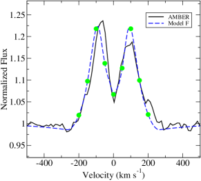
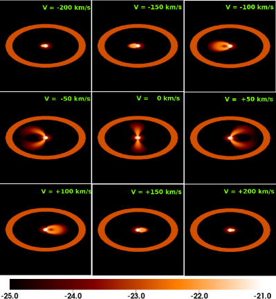
Figure 7: Upper panel: the model Br$\gamma$ profile (dash) computed at $i=55^{\circ}$ with the magnetosphere and disc wind (Model F in Table 6) is compared with the AMBER observation (solid). The velocity channels at which the emission maps (lower panel) are computed are indicated by filled circles. The corresponding emission maps (in logarithmic scale and in arbitrary units) at 9 different velocity channels are shown in the lower panel. The image sizes are 1.89 $\times$ 1.89 $\mathrm{au}^{2}$ or 5.94 $\times$ 5.94 $\mathrm{mas}^{2}$, assuming the object is at 318 pc (VL07). The wavelength/velocity dependent images shown here are used to compute the interferometric quantities such as visibilities, differential phases and closure phases as a function of wavelength/velocity.

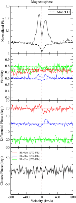
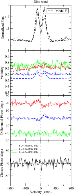
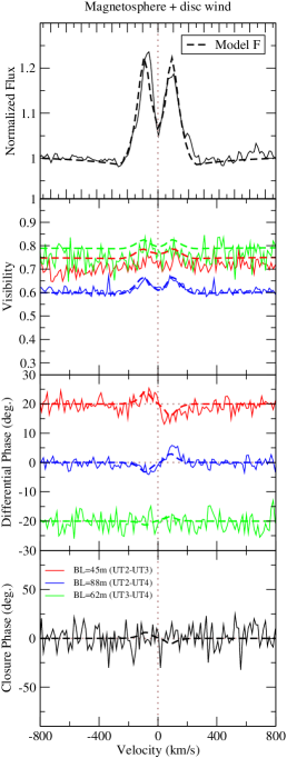
Figure 8: Summary of the model fits to the high-spectral-resolution (R=12000) AMBER observation shown in Fig. 1. The wavelength/velocity-dependent normalised flux, visibilities, differential phases and closure phases are shown from top to bottom. In all the panels, the observed values are shown in solid and the models are in dashed lines. The projected VLTI baselines are 45.4 m (red), 87.9 m (blue) and 62.2 m (green), and their corresponding position angles are $37^{\circ}$, $259^{\circ}$ and $288^{\circ}$, respectively. The differential phases for the first (red) and third (green) baselines are vertically shifted by $+20^{\circ}$ and $-20^{\circ}$, respectively, for clarity. See Fig. 1 for the uncertainties in the absolute calibration of the visibilities. The figure compares three cases: (1) the model with magnetospheric accretion alone (Model D, left panels), (2) the model with the disc wind alone (Model E, middle panels), and (3) the model with a magnetosphere and a disc wind (Model F, right panels). All the models shown here use the inclination angle $i=55^{\circ}$ and the system axis position angle $\mathrm{PA}=85^{\circ}$. Model F (right panels) fits all the observed interferometric quantities well. While Model F shows the best fit to the observations here, the disc wind only model (Model E) could be improved to fit the observations (in particular the visibility levels for the longest baseline) by using a smaller continuum ring radius and by adjusting other model parameters accordingly.

4.3 Modelling spectro-interferometric data

To examine whether the magnetosphere plus disc wind model used to fit the observed Br$\gamma$ line profiles can also fit the other interferometric data obtained by VLTI-AMBER (Fig. 1), we compute the intensity maps of the line-emitting regions plus the ring continuum-emitting region using the same radiative transfer model as in Section 4.2.3. The model intensity maps allow us to compute the wavelength-dependent visibilities, differential and closure phases, and to compare them directly with the observation. As in the geometrical ring fit for the LR VLTI-AMBER continuum visibilities in Section 3, the position angle (PA) of the system is measure from north to east, i.e. the disc/ring normal axis coincides with the north direction when PA is zero, and PA increase as the disc/ring normal axis rotates towards east (cf. Fig. 2).

Examples of the intensity maps computed for Model F (Table 6), with the velocity interval $\Delta v=\,50\mathrm{km~{}s^{-1}}$ between -200 and 200 $\mathrm{km~{}s^{-1}}$, are shown in Fig. 7. Here, the images are computed with $\mathrm{PA}=0\degr$ for a demonstration. The figure also shows the corresponding model Br$\gamma$ profile marked with the same velocity channels used for the images. As expected, the shape of the ring continuum emission does not change across the line, and the emission is uniform. On the other hand, the wind emission size and shape greatly depend on the wavelength/radial velocity. The dependency is consistent with the motion of the gas in the disc wind. The wind base is rotating at the local Keplerian velocities of the accretion disc (between 289 and 78 $\mathrm{km~{}s^{-1}}$ from $R_{\mathrm{wi}}=1.7\,R_{*}$ to $R_{\mathrm{wo}}=23.5\,R_{*}$). As one can see from the figure, the wind on the left-hand side is approaching us, and that on the right-hand side is moving away from us due to the rotational motion of the wind. If the motion of the Br$\gamma$-emitting gas is dominated by the poloidal component, the images would rather have a left-right symmetry. However, this is not the case in our intensity maps. This also indicates that the Br$\gamma$ emission mainly occurs near the base of the wind where the rotational motion dominates. The radial extent of the Br$\gamma$ emission in the disc wind is estimated as $\sim$0.5 au from the intensity maps (with the velocity channels $\pm 50\,\mathrm{km~{}s^{-1}}$ which show the maximum radial extent of the line emission).

By using the emission maps and scaling their sizes according to the distance to HD 58647 (318 pc, VL07), we have computed the wavelength-dependent visibilities, differential and closure phases for Models D, E and F. Here, the maps are computed using the same velocity interval as in the AMBER observations, i.e. $\Delta v\approx 13\,\mathrm{km~{}s^{-1}}$. The computed images are rotated by the PA of the system, which is assumed to be a free parameter. Since the continuum-emitting ring and the disc wind are not spherical symmetric, the visibilities levels, differential and closure phases are sensitive to the PA of the system. Hence, these interferometric data are used as additional constraints for the model fitting procedure with the PA as an additional parameter. The results are summarised in Fig. 8. The figure shows the models computed with the inclination angle $i=55^{\circ}$, the system position angle $\mathrm{PA}=85^{\circ}$ and the continuum-emitting ring radius $R_{\mathrm{Ring}}=23.5\,R_{*}$ for the 3 different cases: (1) the model with magnetospheric accretion only (Model D), (2) the model with the disc wind only (Model E), and (3) the model with a magnetosphere and disc wind (Model F).

In the first case (Model D: with magnetosphere; see Table 6), the agreement of the continuum visibilities with the AMBER observation is excellent, but large disagreements in the line profile shape (as in Sections 4.2.2 and 4.2.3) and the differential phases in the line can be seen. The angular size of the magnetosphere is about 0.15 mas; hence, it is unresolved by the interferometer. There is a slight indication for a depression in the visibility level at the line centre due to the magnetospheric absorption. The photo-centre shifts due to the presence of the magnetosphere are very small on all baselines; hence, there is no change in the differential phases within the line. This clearly disagrees with the observed differential phases which show S-shape signals across the line for two baselines. Similarly, the model closure phases are essentially zero across the line due to the small angular size of the magnetosphere, which is consistent with the observations within in their large error bars ($\sim\pm 20^{\circ}$ as in Fig. 1).

In the second case (Model E: with a disc wind; see Table 6), the agreement of the differential phases with the observation is excellent. This indicates that the disc wind model used here is reasonable. Main disagreements are seen in the line strength and the visibility levels for the longest project baseline (88 m: UT2-UT4). The model Br$\gamma$ line profile is slightly too strong compared to the observed one, and the continuum visibility level for the longest baseline in the model is too low compared to the observation. If we adopt a smaller ring size, the visibility levels for the longest baseline would increase, but the line strength (with respect to the continuum) would also increase. Hence, the disagreement in the line profiles would also increase unless we decrease the line strength by decreasing, for example, the disc wind mass-loss rate ($\dot{M_{\mathrm{dw}}}$). The situation can be improved if there is an additional continuum emission component which is more compact than the ring continuum emission. For example, the continuum emission from the magnetosphere as in the first case (Model D) will make the line weaker and make the visibility slightly larger. A small S-shape variation in closure phases across the line is seen in the model due to the non-spherical symmetric nature of the disc wind emission. The amplitude of the variation is relatively small ($\sim 7^{\circ}$), and it does not disagree with the data which have rather large error bars ($\sim\pm 20^{\circ}$ as in Fig. 1).

In the third case, the model (Model F: with a magnetosphere and disc wind; see Table 6) fits all the observed interferometric quantities, including the line profile, very well. This is our best case of the three models. In particular, the model simultaneously reproduces the following characteristics in the observed interferometric data: (1) the double-peak Br$\gamma$ profile, (1) the double-peak variation of the visibilities across the line (especially for the longest project baseline), (3) the S-shape variations of the differential phases across the line, and (4) the small amplitude in the variation of the closure phases across the line. The locations of the peaks in the visibilities curves are approximately $\pm 50\,\mathrm{km~{}s^{-1}}$, which corresponds to the two peaks in the line profile. The line emission maps shown earlier (Fig. 7) also suggests that the extent of the line emission from the disc wind is largest at these velocities.

In summary, our radiative transfer model (Model F in Table 6), which uses a combination of a small magnetosphere and a disc wind with its inner radius at the outer radius of the magnetosphere, is in good agreement with the observed interferometric data for HD 58647. The extent of the line-emitting disc wind region (the outer radius of the intensity distribution $\sim 0.5$ au as in Fig. 7) is slightly smaller than the K-band continuum-emitting ring size ($R_{\mathrm{ring}}=23.5\,R_{*}$ or 0.68 au) which approximately corresponds to the dust sublimation radius of the system.

5 Discussion

5.1 Continuum-emitting regions

In Section 3, we used a simple geometrical model (an elongated ring) and the observed continuum visibilities to estimate the size of the K-band continuum-emitting region. The angular radius of the ring emission was estimated as $R_{\mathrm{ring}}=2.0$ mas or equivalently 0.64 au at the distance of 318 pc (VL07) (Table 4). This radius is slightly larger than the value obtained by MO05, i.e. $1.47$ mas. However, their radius determination does not include the effect of ring elongation/inclination because the $uv$-coverage of the Keck Interferometer in MO05 provides almost no two-dimensional information. Further, the ring radius estimated in Section 3 (0.64 au) is slightly smaller than the value used in the radiative transfer models (Table 6), i.e. $R_{\mathrm{ring}}=0.68$ au. The larger continuum radius is used in the radiative transfer model to reproduced the observed visibilities because of the additional compact continuum emission from the magnetosphere, which is not included in the geometric model in Section 3.

Assuming a dust sublimation temperature of 1500 K and the stellar luminosity of $L_{*}=412\,\mathrm{L_{\sun}}$ (Section 4.2.1), the size-luminosity relationship in MO05 provides a dust sublimation radius $R_{\mathrm{s}}$ of $0.64$ au. This is very similar to the ring radius $R_{\mathrm{ring}}=0.68$ au used in the radiative transfer model (Model F), which fits our AMBER continuum visibility observation (Fig. 8).

5.2 Disc wind launching regions

According to the disc wind model (Model F), which fits the spectro-interferometric observation in Section 4.3 well, the inner radius of the disc-wind launching region ($R_{\mathrm{wi}}$) is only 0.05 au, which is located just outside of the magnetosphere. This radius is much smaller than the dust sublimation radius ($R_{\mathrm{s}}$), which is approximately equal to the radius of the continuum-emitting geometrical ring $R_{\mathrm{ring}}=0.68$ au, as shown in the previous section. Next, we compare the size of the inner radius of the disc-wind launching region of our HD 58647 model with those found in earlier studies of other Herbig Ae/Be stars, in which the VLTI-AMBER in the high spectral resolution mode and radiative transfer models for Br$\gamma$ were used. Only three such studies are available in the literature: the Herbig Be star MWC 297 (Weigelt et al. 2011), the Herbig Ae star MWC 275 (Garcia Lopez et al. 2015) and the Herbig Be star HD 98922 (Caratti o Garatti et al. 2015). These studies used similar kinematic disc wind models to probe the wind-launching region of these stars. Fig. 9 shows the inner radii of the disc wind launching regions plotted as a function of stellar luminosity (see also Table 8). The figure shows that the inner radius of the wind launching region increases as the luminosity increases. By fitting the data with a power-law, we find the following relation:

$$\left(\frac{R_{\mathrm{wi}}}{1\,\mathrm{au}}\right)=a\left(\frac{L_{*}}{1\,\mathrm{L_{\sun}}}\right)^{b}$$ (3)

where $a=2.0(^{+1.1}_{-0.7})\times 10^{-3}$ and $b=0.59(\pm 0.07)$. As in Table 8, the inner radius of the wind launching region is only a few times larger than the stellar radius ($1.7$–$3.0\,R_{*}$) for MWC 275, HD 98922 and HD 58647, which have similar spectral types (A1 and B9). On the other hand, it is much larger ($R_{\mathrm{wi}}=17.5\,R_{*}$) for MWC 297 which has a much earlier spectral type (B1.5). This may suggest that the environment of the wind-launching regions in MWC 297 might be different from those in MWC 275, HD 98922 and HD 58647. The difference between the wind-launching region of MWC 297 and those of the lower luminosity stars may be caused by the difference in the strength of stellar and/or disc radiation (pressure) which may influence the wind launching radius and wind dynamics (e.g. Drew et al. 1997; Proga, Stone, & Drew 1999).

The physical origin of the relation in equation 3 is unknown. The increase in $R_{\mathrm{wi}}$ for the stars with lower luminosities (MWC 275, HD 98922 and HD 58647) may simply reflect the increase in their stellar radii (the fourth column in Table 8), which, in turn, set the size of magnetospheric radius or the inner radius of the accretion disc from which the wind arises. The cause of the increase in $R_{\mathrm{wi}}$ from the three stars with lower luminosities (MWC 275, HD 98922 and HD 58647) to MWC 297 is even more uncertain since the stellar radius of MWC 297 is not significantly larger than the others.

Another difference between MWC 297 and the other three stars in our sample can be found in their K-band continuum emission radii. Fig. 9 also shows the radius of the K-band continuum-emitting ring for each object along with the expected dust sublimation radii (assuming the dust sublimation temperature of 1500 K) computed from the size-luminosity relation in MO05. While the ring radii of MWC 275, HD 98922 and HD 58647 follow the expected size-luminosity relation, that of MWC 297 falls below the expected value for the dust sublimation temperature of 1500 K. The continuum ring radius is about 10 times larger than the inner radius of the disc wind in MWC 275, HD 98922 and HD 58647, but it is only 1.1 times larger for the luminous MWC 297. The tendency for the high luminosity Herbig Be stars ($L_{*}>10^{3}\,\mathrm{L_{\sun}}$) to have an ‘undersized’ dust sublimation radius is pointed out by MO05. They suggest that the innermost gas accretion disc might be optically thick for luminous Herbig Be stars, and it partially blocks the stellar radiation on to the disc, hence causing a smaller dust sublimation radius (see also Eisner et al. 2004).

The outflow, from which the observed Br$\gamma$ emission line originates, is most likely formed in magnetohydrodynamical processes, in either (1) magneto-centrifugal disc wind (e.g. Blandford & Payne 1982; Ouyed & Pudritz 1997; Krasnopolsky et al. 2003) or (2) a wind launched near the disc-magnetosphere interaction region (e.g. an X-wind – Shu et al. 1994, 1995 or a conical wind – Romanova et al. 2009). The (accretion-powered) stellar wind (e.g. Decampli 1981; Hartmann & MacGregor 1982; Strafella et al. 1998; Matt & Pudritz 2005; Cranmer 2009) is unlikely the origin of Br$\gamma$ emission line in the case of HD 58647 because the line computed with such a wind would have a single-peaked profile while the observed Br$\gamma$ is double-peaked with its peak separation of $\sim 160\,\mathrm{km~{}s^{-1}}$ (Fig. 1). Our radiative transfer model uses a simple disc wind plus a compact magnetosphere, and we have demonstrated that this model is able to reproduce the interferometric observation with the VLTI-AMBER (Fig. 8). However, the disc wind in this model could also resemble the flows found in the conical wind and X-wind models, in which the mass ejection region is also concentrated just outside of a magnetosphere. This is because the inner radius of the disc wind model (Model F in Table 6) is also located just outside of the magnetosphere. Further, the local mass-loss rate ($\dot{m}$, the mass-loss rate per unit area) on the accretion disc in our model is a strong function of $w$ (the distance from the star on the accretion disc plane), i.e. $\dot{m}\propto w^{-2.4}$. Thus, the mass-loss flux is concentrated just outside of the magnetosphere as in the conical and X-wind models. It would be difficult to exclude the conical or X-wind as a possible outflow model in this case. Only when the inner radius of the wind launching region is significantly larger than the corotation radius of a star (as in MWC 297, Table 8), they could be safely excluded.

Finally, the rate of angular momentum loss by the disc wind ($\dot{J}_{\mathrm{dw}}$) can be directly calculated in our model (Models E and F) because we adopted the explicit forms of the mass-loss rate per unit area and the wind velocity law (Section 4.1.3). In the context of a magneto-centrifugal disc wind model, the specific angular momentum ($j$) transported along each magnetic field line can be written as

$$j=\left(r_{\mathrm{A}}/r_{0}\right)^{2}\,j_{0}$$ (4)

(e.g. Pudritz et al. 2007) where $r_{A}$ and $r_{0}$ are the Alfvén radius and the wind launching radius, respectively, whereas $j_{0}$ is the specific angular momentum of the disc at $r_{0}$. Here, we assume $(r_{A}/r_{0})\approx 3$ as in Pudritz et al. (2007). Using the total wind mass-loss rate found in the Models E and F ($\dot{M}_{\mathrm{dw}}=4.5\times 10^{-8}\,\mathrm{M_{\sun}\,yr^{-1}}$, Table 6) as the normalization constant, we can integrate the angular momentum carried away by the wind over the whole wind launching area (from $R_{\mathrm{wi}}=1.7\,R_{*}$ to $R_{\mathrm{wo}}=23.5\,R_{*}$) to obtain the rate of the total angular momentum loss by the disc wind ($\dot{J}_{\mathrm{dw}}$). We find this value as $\dot{J}_{\mathrm{dw}}=9.9\times 10^{38}$ erg.

On the other hand, the rate of angular momentum loss ($\dot{J}_{\mathrm{disc}}$) that is required at the disc wind outer radius $R_{\mathrm{wo}}$ to maintain a steady accretion in the Keplerian disc with a mass-accretion rate $\dot{M}_{\mathrm{a}}$ is

$$\dot{J}_{\mathrm{disc}}=\dot{M}_{\mathrm{a}}\,j_{\mathrm{wo}}=\dot{M}_{\mathrm{a}}\,\left(GM_{*}\,R_{\mathrm{wo}}\right)^{1/2}$$ (5)

where $j_{\mathrm{wo}}$ is the specific angular momentum of the gas at the disc wind outer radius $R_{\mathrm{wo}}$ (e.g. Pudritz & Ouyed 1999). Using the mass-accretion rate for HD 58647, $\dot{M}_{\mathrm{a}}=3.5\times 10^{-7}\,\mathrm{M_{\sun}\,yr^{-1}}$ (Table 5), we find $\dot{J}_{\mathrm{disc}}=1.7\times 10^{39}$ erg. Hence, the ratio $\dot{J}_{\mathrm{dw}}/\dot{J}_{\mathrm{disc}}$ is about 0.58. Interestingly, this is very similar to the ratio found by Bacciotti et al. (2002) in the observation of the classical T Tauri star DG Tau.

Our model suggests that about 60 per cent of the angular momentum loss rate is in the disc wind. This in turn indicates that the disc wind plays a significant role in the angular momentum transport, and it dominates the role of the X-wind (if coexists) since the rate of angular momentum loss by the latter is expected to be much smaller (e.g. Ferreira et al. 2006).

Table 8: The inner radii of disc wind launching regions ($R_{\mathrm{wi}}$) and the continuum-emitting ring ($R_{\mathrm{ring}}$) of the Herbig Ae/Be stars observed with the VLTI-AMBER in the high spectral resolution mode (including this study).

Object	Sp. type	$L_{*}$	$R_{*}$	$R_{\mathrm{wi}}$		$R_{\mathrm{ring}}$		References
	$\cdots$	($\mathrm{L_{\sun}}$)	($\mathrm{R_{\sun}}$)	(au)	($R_{*}$)	(au)	($R_{*}$)
MWC 275	A1 V	$40^{b}$	$2.3^{a}$	$0.02^{a}$	$2.0^{a}$	$0.23^{b}$	$21.5^{b}$	aGarcia Lopez et al. (2015), bMonnier et al. (2005)
HD 58647	B9 IV	$412$	$6.2$	$0.05$	$1.7$	$0.68$	$23.5$	This work
HD 98922	B9 V	$640$	$7.6$	$0.1$	$3.0$	$0.7$	$19.8$	Caratti o Garatti et al. (2015)
MWC 297	B1.5V	$10600$	$6.1$	$0.5$	$17.5$	$0.56$	$19.7$	Weigelt et al. (2011)

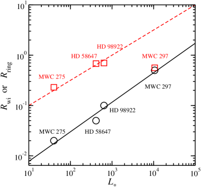
Figure 9: Comparison of the disc wind inner radii ($R_{\mathrm{wi}}$) for the Herbig Ae/Be stars observed with the VLTI-AMBER in the high spectral resolution mode: MWC 275 (Garcia Lopez et al. 2015), HD 58647 (this work), HD 98922 (Caratti o Garatti et al. 2015) and MWC 297 (Weigelt et al. 2011). The inner radii of the disc wind used in radiative transfer models (circle) are shown as a function of stellar luminosity ($L_{*}$). The slope of the power-law fit (solid) for the disc wind inner radii is $0.59(\pm 0.07)$. The radius of the K-band continuum-emitting ring ($R_{\mathrm{ring}}$, square) and the expected dust sublimation radii from MO05 (dash, assuming the dust sublimation temperature of 1500 K) are also shown for a comparison. The units for the radii ($R_{\mathrm{wi}}$ and $R_{\mathrm{ring}}$) and the luminosity ($L_{*}$) are in au and $\mathrm{L_{\sun}}$, respectively. See Table 8 for the numerical values used for this plot.

5.3 Is there a magnetosphere in HD 58647?

The presence of a magnetosphere in HD 58647 is suggested by a variety of observations. For example, the spectroscopic study of HD 58647 by Mendigutía et al. (2011) shows a hint for an inverse P-Cygni profile or a redshifted absorption component in He i 5876 Å, which might be formed in a magnetospheric accretion funnel. Interestingly, a recent spectroscopic survey of Herbig Ae/Be stars by Cauley & Johns-Krull (2015) has shown that about 14 per cent of their samples exhibit the inverse P-Cygni profile in He i 5876 Å (see also Cauley & Johns-Krull 2014). Further, the spectropolarimetic (linear) observation of H$\alpha$ in HD 58647 by Vink et al. (2002), Mottram et al. (2007) and Harrington & Kuhn (2009) show a large polarization change in the line and the pattern on the Stokes parameter $QU$ plane is a loop — indicating that a part of H$\alpha$ emission is intrinsically polarized and the emission is scattered by the gas with a flattened geometry. A similar pattern on the $QU$ plane are also seen in the classical T Tauri stars and Herbig Ae stars. Mottram et al. (2007) suggested that the intrinsically polarized H$\alpha$ (at least partially) originates from a magnetosphere. Lastly, a recent spectropolarimetric observation by Hubrig et al. (2013) showed that the star has a mean longitudinal magnetic field with strength <$B_{z}$>=$218\pm 69$ G, supporting a possible presence of a magnetosphere in HD 58647.

Based on these evidences, a magnetosphere with a small radius was introduced in the radiative transfer models for the Br$\gamma$ line profile and the interferometric data (Sections 4.2 and 4.3). In Sections 4.2, we found that the small magnetosphere does not significantly contribute to the Br$\gamma$ line emission (Fig. 5). On the other hand, we find the disc wind is the main contributor for the Br$\gamma$ emission in HD 58647 (Fig. 6). Since the mass-accretion rate of HD 58647 is relatively high ($\dot{M}_{\mathrm{a}}=3.5\times 10^{-7}\,\mathrm{M_{\sun}\,yr^{-1}}$, Brittain et al. 2007), it may contribute a non-negligible amount of continuum flux in the K-band. For example, in Model F, approximately 10 per cent of the total continuum flux is from the magnetosphere. This has at least two consequences: (1) the normalized line profile will be slightly weaker because of the larger total continuum flux (Fig. 6), and (2) the continuum visibilities would be larger since the magnetosphere is unresolved (its continuum emission is compact) (Fig. 8). In other words, we might slightly underestimate e.g. the disc wind mass-loss rate if a magnetosphere is not included in the model since it would produce a slightly stronger line (due to a weaker continuum). We might also slightly underestimate the size for the continuum-emitting ring when the magnetosphere is not included in the model. A slightly larger ring size is needed to balance the increase in the visibility due to the emission from the magnetosphere.

One can estimate the dipolar magnetic field strength of HD 58647 at the magnetic equator ($B_{*}$) using the standard relation between the dipole magnetic field strength and stellar parameters found in Königl (1991) and Johns-Krull, Valenti, & Koresko (1999), i.e.

$$B_{*} = K\left(\frac{\epsilon}{0.35}\right)^{7/6}\left(\frac{\beta}{0.5}\right)^{-7/4}\left(\frac{M_{*}}{\mathrm{M_{\sun}}}\right)^{5/6}$$ (7)

$$\times\left(\frac{\dot{M}_{\mathrm{a}}}{10^{-7}\,\mathrm{M_{\sun}\,yr^{-1}}}\right)^{1/2}\left(\frac{R_{*}}{\mathrm{R_{\sun}}}\right)^{-3}\left(\frac{P_{*}}{1.0\,\mathrm{d}}\right)^{7/6}$$

where $K$ is a constant: $3.43\times 10^{3}\,\mathrm{G}$. The parameters $\beta$ and $\epsilon$ represent the efficiency of the coupling between the stellar magnetic field and the inner regions of the disc, and the ratio of the stellar angular velocity to the Keplerian angular velocity at the inner radius of a magnetosphere, respectively. Here, we adopt $\beta=0.5$ and $\epsilon=0.35$, as in Königl (1991) and Johns-Krull et al. (1999). By using the stellar parameters used in our model (Table 5) in equation 7, we find $B_{*}=240$ G. This is very similar to the mean longitudinal magnetic field strength <$B_{z}$>=$218\pm 69$ G found in the spectropolarimetric observations of HD 58647 by Hubrig et al. (2013).

5.4 A Keplerian disc as a main source of Br$\gamma$ emission?

So far, we have argued that the double-peaked Br$\gamma$ emission line profile seen in HD 58647 is mainly formed in a disc wind, which is rotating near Keplerian velocity at the base of the wind. The model with a disc wind and a magnetosphere (Model F in Fig. 8) was also able to reproduce the interferometric observations by VLTI-AMBER. However, the double-peaked Br$\gamma$ line profile could be also formed in a gaseous Keplerian disc (without a disc wind), as often demonstrated in the models for (more evolved) classical Be stars (e.g. Carciofi & Bjorkman 2008; Kraus et al. 2012c; Meilland et al. 2012; Rivinius et al. 2013). In addition, we find that the emission maps computed for different velocity channels across Br$\gamma$ shown in Fig. 7 is rather similar to those computed with a simple Keplerian disc (e.g. Kraus et al. 2012c; Mendigutía et al. 2015). The similarity naturally occurs because the Br$\gamma$ emission in our disc wind model arises mainly from near the base of the wind where the Keplerian rotation of the wind is dominating over the poloidal motion. For this reason, it would be difficult to exclude a simple Keplerian disc as a main source of the Br$\gamma$ emission in HD 58647 based solely on our VLTI-AMBER observations.

Fig. 10 shows the poloidal and azimuthal velocity components of the disc wind at its base for Model F, plotted as a function of the distance from the symmetric/rotation axis. The corresponding density at the base of the disc wind is also shown in the same figure as a reference. In our model, the poloidal speed of the disc wind ($v_{\mathrm{p}}$) is set by equation 2 in Section 4.1.3. The poloidal speed of the wind at its base can be found by setting $l=0$ in the equation, i.e. $v_{\mathrm{p}}(w_{i},l=0)=c_{\mathrm{s}}(w_{i})$ where $c_{\mathrm{s}}(w_{i})$ the local sound speed, and $w_{i}$ is the distance from the symmetry/rotation axis. Hence, the poloidal speed at the base of the wind is equal to the local sound speed. The sound speed at the inner disc wind launching radius ($R_{\mathrm{wi}}=1.7\,R_{*}$) is about 4 $\mathrm{km~{}s^{-1}}$ (assuming $T\sim 2000$ K as in Muzerolle et al. 2004). This is significantly smaller than the (wind) Keplerian speed at the same location, i.e. 289 $\mathrm{km~{}s^{-1}}$. Although not shown here, as a simple test, we computed Br$\gamma$ line profiles using exactly the same density distribution as in Model F (magnetosphere + disc wind), but with $v_{\mathrm{p}}$ manually boosted by a constant factor to examine how large $v_{\mathrm{p}}$ should be for the Br$\gamma$ line profile to show a line asymmetry or a deviation from the Keplerian velocity dominated Br$\gamma$ line profile seen in Model F. In this experiment, we found that the Br$\gamma$ line profile started to show the effect of $v_{\mathrm{p}}$ when it was boosted by a factor of $\sim 5$. The corresponding $v_{\mathrm{p}}$ at the base of the wind at the inner wind radius ($R_{\mathrm{wi}}$) is about 25 $\mathrm{km~{}s^{-1}}$. In the original disc wind velocity distribution (without the boosting factor), $v_{\mathrm{p}}$ can reach 25 $\mathrm{km~{}s^{-1}}$ at about 2 $R_{*}$ away from the wind launching point along the streamline emerging from the inner disc wind radius ($R_{\mathrm{wi}}$). If the Br$\gamma$ emission mainly arose from this region or a location farther away from the launching point, we would be able to see the effect of the poloidal velocity. However, this is not the case for our model (Model F), i.e. the Br$\gamma$ emission seems to originate much closer to the disc surface.

As seen in Section 4.2.3, to produce a Br$\gamma$ emission line with its strength comparable to the one seen in the observation, the temperature of the gas must be rather high ($\sim 10^{4}$ K) and the emission volume must be sufficiently large. In the study of thermal properties of Keplerian discs (without a disc wind) around classical Be star, Carciofi & Bjorkman (2006) showed that the gas temperature in the upper layers of discs could reach $\sim 10^{4}$ K, although they considered stars with $T_{\mathrm{eff}}=19000$ K which is much higher than that for HD 58647 ($T_{\mathrm{eff}}=10500$ K, Table 5). It is uncertain if the same model is applicable to HD 58647 and if it can produce gas with high enough temperature ($\sim 10^{4}$ K) using the stellar parameters of HD 58647. Furthermore, in the study of the thermal property of gaseous discs irradiated by Herbig Ae/Be stars, Muzerolle et al. (2004) found the gas temperatures in the upper layers of accretion discs were relatively low ($\sim$2000 K). This is certainly too low for the formation of a Br$\gamma$ emission line. On the other hand, the disc wind gas has favorable conditions for Br$\gamma$ emission because of the acceleration and heating of the gas in the disc wind by e.g. ambipolar diffusion (e.g. Safier 1993; Garcia et al. 2001) and internal jet shocks (e.g. Staff et al. 2010), which can bring the temperature to $\sim 10^{4}$ K.

To compute the emission line profiles from a Keplerian disc with self-consistent density and temperature structures (by considering hydrostatic and radiative equilibriums), we would need a major change in our model. This is beyond the scope of this paper; however, it should be investigated in the future in detail. Only then, we would be able to address the issue of distinguishing interferometric signatures of a disc wind from those of a simple Keplerian disc.

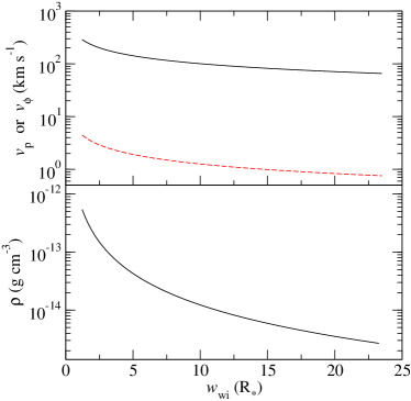
Figure 10: A comparison of the velocity components (upper panel) and density (lower panel) at the base of the disc wind model used in Model F. The poloidal (dash) and Keplerian (solid) velocity components ($v_{\mathrm{p}}$ and $v_{\phi}$, respectively) are plotted as a function of the distance ($w_{i}$) from the symmetric/rotation axis. The range of $w_{i}$ is from $R_{\mathrm{wi}}=1.7\,R_{*}$ to $R_{\mathrm{wo}}=23.5\,R_{*}$ as in Model F (Table 6). The poloidal speed of the disc wind at the base is calculated by setting $l=0$ in equation 2 in Section 4.1.3. The corresponding density ($\rho$) of the disc wind is computed using equation 6 in Kurosawa et al. (2006). The Keplerian component dominates the poloidal component at all the wind launching radii. The wind density at the base decreases from $\sim 5\times 10^{-13}$ to $\sim 3\times 10^{-15}\,\mathrm{g\,cm^{-3}}$ as the wind launching radius increases.

6 Conclusions

We have presented a study of the wind-launching region of the Herbig Be star HD 58647 using high angular and high spectral ($R=12000$) resolution interferometric observations of the Br$\gamma$ line-emitting region. The high spectral resolution of AMBER provides us many spectral channels across the line to investigate the wind origin and properties of HD 58647 (Fig. 1). The star displays double peaks in Br$\gamma$ and in the wavelength-dependent visibility curves. The differential phase curves show S-shaped variations around the line centre.

Based on a simple geometrical ring fit for the continuum visibilities (Fig. 3), we find the K-band continuum-emitting ring size is around 2.0 mas, which corresponds to 0.64 au at the distance of 318 pc (VL07). The visibility level increases in the line (by $\sim 0.1$) for the longest project baseline (88 m), indicating that the extent of the Br$\gamma$ emission region is smaller than the size of the continuum-emitting region, which is expected to arise near the dust sublimation radius of the accretion disc.

The interferometric data have been analysed using radiative transfer models to study the geometry, size and physical properties of the wind. The double-peaked line profile and the pattern of the differential phase curves (S-shaped) suggest that the line-emitting gas is rotating. We find that a model with a small magnetosphere with outer radius $R_{\mathrm{mo}}=1.7\,R_{*}$ plus a disc wind with the inner radius located just outside of the magnetosphere and outer radius $R_{\mathrm{wo}}=22.5\,R_{*}$ (Model F) can fit the observed Br$\gamma$ profile, wavelength-dependent visibilities, differential and closure phases, simultaneously (Fig. 8). The model has shown that the radial extent of the Br$\gamma$ emission in the disc wind is about 0.5 au while the inner radius of the K-band continuum-emitting ring is about 0.68 au (Fig. 7). The slightly larger size of the continuum ring emission, compared to the one obtained in the simple geometrical model (Section 3), is found in the radiative transfer model because it includes the continuum emission from the compact magnetosphere ($\sim$ 10 per cent of the total K-band flux). The mass-accretion and mass-loss rates adopted for the model are $3.5\times 10^{-7}$ and $4.5\times 10^{-8}\,\mathrm{M_{\sun}\,yr^{-1}}$, respectively ($\dot{M}_{\mathrm{dw}}/\dot{M}_{\mathrm{a}}=0.13$). Consequently, about 60 per cent of the angular momentum loss rate required for a steady accretion with the measured accretion rate is provide by the disc wind (Section 5.2).

We find that the small magnetosphere does not contribute significantly to the Br$\gamma$ line emission significantly (Fig. 6). The size of the innermost radius in the disc wind model (Model F) was compared with those from the earlier studies Herbig Ae/Be stars with high spectral resolution VLTI-AMBER observations (Weigelt et al. 2011; Garcia Lopez et al. 2015; Caratti o Garatti et al. 2015). We found a trend that the inner radius of the wind-launching region increases as the luminosity of a star increases (Fig. 9).

While the model with a disc wind plus magnetosphere (Model F) showed the best fit to the interferometric observations (Fig. 8), the disc wind only model (Model E) could be improved to fit the observations (in particular the visibility levels for the longest baseline) by using a smaller continuum ring radius and by adjusting other model parameters accordingly. Hence, the model proposed here (Model F) is not necessary a unique fit to the observations.

As briefly mentioned in Section 5.2, the AMBER observation could be also explained by the conical wind (e.g. Romanova et al. 2009) or X-wind (e.g. Shu et al. 1994) models because the disc wind model that fits the AMBER observation has an inner radius comparable to the size of the magnetosphere, and its mass-loss is also concentrated near the disc-magnetosphere interaction region, as in the conical and X-wind models. However, the X-wind model alone might have a difficulty in explaining the rate of the angular momentum loss required for a steady accretion in the Keplerian disc (Section 5.2). Also, as mentioned in Section 5.4, we still cannot exclude a simple Keplerian disc model as a main source of the Br$\gamma$ emission in HD 58647 since the model could produce a double-peaked Br$\gamma$ emission line and could produce similar velocity-dependent emission maps to those computed with a disc wind (Fig 7).

In the future, we need a systematic study to find how the interferometric signatures differ in different outflow models, perhaps by using the results of MHD simulations. To improve our understanding of the wind properties (e.g. temperature), it would be useful to combine the interferometric observations with high-resolution spectroscopic observations. Simultaneous fitting of multiple emission lines in the spectroscopic observations would provide us tighter constrains on the physical properties of the gas in the wind. To improve the interferometric data, we would need higher signal-to-noise data under good seeing condition and a larger coverage on the $uv$ plane.

References

- Alencar et al. (2012) Alencar S. H. P., Bouvier J., Walter F. M., Dougados C., Donati J.-F., Kurosawa R., Romanova M., Bonfils X., Lima G. H. R. A., Massaro S., Ibrahimov M., Poretti E., 2012, A&A, 541, A116
- Bacciotti et al. (2002) Bacciotti F., Ray T. P., Mundt R., Eislöffel J., Solf J., 2002, ApJ, 576, 222
- Bayo et al. (2008) Bayo A., Rodrigo C., Barrado Y Navascués D., Solano E., Gutiérrez R., Morales-Calderón M., Allard F., 2008, A&A, 492, 277
- Benisty et al. (2010) Benisty M., Malbet F., Dougados C., Natta A., Le Bouquin J. B., Massi F., Bonnefoy M., Bouvier J., Chauvin G., Chesneau O., Garcia P. J. V., Grankin K., Isella A., Ratzka T., Tatulli E., Testi L., Weigelt G., Whelan E. T., 2010, A&A, 517, L3
- Berthoud et al. (2007) Berthoud M. G., Keller L. D., Herter T. L., Richter M. J., Whelan D. G., 2007, ApJ, 660, 461
- Blandford & Payne (1982) Blandford R. D., Payne D. G., 1982, MNRAS, 199, 883
- Bouvier et al. (2014) Bouvier J., Matt S. P., Mohanty S., Scholz A., Stassun K. G., Zanni C., 2014, in Protostars and Planets VI, Beuther H., Klesser R., Dullemond K., Henning T., eds., Univ. Arizona Press, Tuscon, p. 433
- Brittain et al. (2007) Brittain S. D., Simon T., Najita J. R., Rettig T. W., 2007, ApJ, 659, 685
- Caratti o Garatti et al. (2015) Caratti o Garatti A., Tambovtseva L. V., Garcia Lopez R., Kraus S., Schertl D., Grinin V. P., Weigelt G., Hofmann K.-H., Massi F., Lagarde S., Vannier M., Malbet F., 2015, A&A, 582, A44
- Carciofi & Bjorkman (2006) Carciofi A. C., Bjorkman J. E., 2006, ApJ, 639, 1081
- Carciofi & Bjorkman (2008) —, 2008, ApJ, 684, 1374
- Castor (1970) Castor J. I., 1970, MNRAS, 149, 111
- Castor & Lamers (1979) Castor J. I., Lamers H. J. G. L. M., 1979, ApJS, 39, 481
- Cauley & Johns-Krull (2014) Cauley P. W., Johns-Krull C. M., 2014, ApJ, 797, 112
- Cauley & Johns-Krull (2015) —, 2015, ApJ, 810, 5
- Chelli et al. (2009) Chelli A., Utrera O. H., Duvert G., 2009, A&A, 502, 705
- Cranmer (2009) Cranmer S. R., 2009, ApJ, 706, 824
- Cutri et al. (2003) Cutri R. M., Skrutskie M. F., van Dyk S., Beichman C. A., Carpenter J. M., Chester T., Cambresy L., Evans T., Fowler J., Gizis J., et al., 2003, VizieR Online Data Catalog, 2246
- Decampli (1981) Decampli W. M., 1981, ApJ, 244, 124
- Drew et al. (1997) Drew J. E., Busfield G., Hoare M. G., Murdoch K. A., Nixon C. A., Oudmaijer R. D., 1997, MNRAS, 286, 538
- Dullemond & Monnier (2010) Dullemond C. P., Monnier J. D., 2010, ARA&A, 48, 205
- Edwards et al. (2006) Edwards S., Fischer W., Hillenbrand L., Kwan J., 2006, ApJ, 646, 319
- Eisner et al. (2014) Eisner J. A., Hillenbrand L. A., Stone J. M., 2014, MNRAS, 443, 1916
- Eisner et al. (2004) Eisner J. A., Lane B. F., Hillenbrand L. A., Akeson R. L., Sargent A. I., 2004, ApJ, 613, 1049
- Eisner et al. (2010) Eisner J. A., Monnier J. D., Woillez J., Akeson R. L., Millan-Gabet R., Graham J. R., Hillenbrand L. A., Pott J.-U., Ragland S., Wizinowich P., 2010, ApJ, 718, 774
- Ellerbroek et al. (2015) Ellerbroek L. E., Benisty M., Kraus S., Perraut K., Kluska J., le Bouquin J. B., Borges Fernandes M., Domiciano de Souza A., Maaskant K. M., Kaper L., Tramper F., Mourard D., Tallon-Bosc I., ten Brummelaar T., Sitko M. L., Lynch D. K., Russell R. W., 2015, A&A, 573, A77
- Ferreira et al. (2006) Ferreira J., Dougados C., Cabrit S., 2006, A&A, 453, 785
- Garcia et al. (2001) Garcia P. J. V., Ferreira J., Cabrit S., Binette L., 2001, A&A, 377, 589
- Garcia Lopez et al. (2016) Garcia Lopez R., Kurosawa R., Caratti o Garatti A., Kreplin A., Weigelt G., Tambovtseva L. V., Grinin V. P., Ray T. P., 2016, MNRAS, 456, 156
- Garcia Lopez et al. (2015) Garcia Lopez R., Tambovtseva L. V., Schertl D., Grinin V. P., Hofmann K.-H., Weigelt G., Caratti o Garatti A., 2015, A&A, 576, A84
- Ghosh et al. (1977) Ghosh P., Pethick C. J., Lamb F. K., 1977, ApJ, 217, 578
- Grady et al. (1996) Grady C. A., Perez M. R., Talavera A., Bjorkman K. S., de Winter D., The P.-S., Molster F. J., van den Ancker M. E., Sitko M. L., Morrison N. D., Beaver M. L., McCollum B., Castelaz M. W., 1996, A&AS, 120, 157
- Harries (2000) Harries T. J., 2000, MNRAS, 315, 722
- Harrington & Kuhn (2009) Harrington D. M., Kuhn J. R., 2009, ApJS, 180, 138
- Hartmann et al. (1994) Hartmann L., Hewett R., Calvet N., 1994, ApJ, 426, 669
- Hartmann & MacGregor (1982) Hartmann L., MacGregor K. B., 1982, ApJ, 257, 264
- Hartmann & Stauffer (1989) Hartmann L., Stauffer J. R., 1989, AJ, 97, 873
- Hauschildt & Baron (1999) Hauschildt P. H., Baron E., 1999, J. Comput. Appl. Math., 109, 41
- Haworth & Harries (2012) Haworth T. J., Harries T. J., 2012, MNRAS, 420, 562
- Herbst et al. (2002) Herbst W., Bailer-Jones C. A. L., Mundt R., Meisenheimer K., Wackermann R., 2002, A&A, 396, 513
- Herbst et al. (1987) Herbst W., Booth J. F., Koret D. L., Zajtseva G. V., Shakhovskaya H. I., Vrba F. J., Covino E., Terranegra L., Vittone A., Hoff D., Kelsey L., Lines R., Barksdale W., 1987, AJ, 94, 137
- Herbst et al. (1994) Herbst W., Herbst D. K., Grossman E. J., Weinstein D., 1994, AJ, 108, 1906
- Hirose et al. (1997) Hirose S., Uchida Y., Shibata K., Matsumoto R., 1997, PASJ, 49, 193
- Hubrig et al. (2013) Hubrig S., Ilyin I., Schöller M., Lo Curto G., 2013, Astron. Nachr., 334, 1093
- Hubrig et al. (2011) Hubrig S., Mikulášek Z., González J. F., Schöller M., Ilyin I., Curé M., Zejda M., Cowley C. R., Elkin V. G., Pogodin M. A., Yudin R. V., 2011, A&A, 525, L4
- Hubrig et al. (2009) Hubrig S., Stelzer B., Schöller M., Grady C., Schütz O., Pogodin M. A., Curé M., Hamaguchi K., Yudin R. V., 2009, A&A, 502, 283
- Husser et al. (2013) Husser T.-O., Wende-von Berg S., Dreizler S., Homeier D., Reiners A., Barman T., Hauschildt P. H., 2013, A&A, 553, A6
- Johns-Krull et al. (1999) Johns-Krull C. M., Valenti J. A., Koresko C., 1999, ApJ, 516, 900
- Knigge et al. (1995) Knigge C., Woods J. A., Drew J. E., 1995, MNRAS, 273, 225
- Königl (1991) Königl A., 1991, ApJ, 370, L39
- Königl & Pudritz (2000) Königl A., Pudritz R. E., 2000, in Protostars and Planets IV, Mannings V., Boss A. P., Russell S., eds., Univ. Arizona Press, Tuscon, p. 759
- Krasnopolsky et al. (2003) Krasnopolsky R., Li Z.-Y., Blandford R. D., 2003, ApJ, 595, 631
- Kraus et al. (2012a) Kraus S., Calvet N., Hartmann L., Hofmann K.-H., Kreplin A., Monnier J. D., Weigelt G., 2012a, ApJ, 746, L2
- Kraus et al. (2012b) —, 2012b, ApJ, 752, 11
- Kraus et al. (2008) Kraus S., Hofmann K.-H., Benisty M., Berger J.-P., Chesneau O., Isella A., Malbet F., Meilland A., Nardetto N., Natta A., Preibisch T., Schertl D., Smith M., Stee P., Tatulli E., Testi L., Weigelt G., 2008, A&A, 489, 1157
- Kraus et al. (2012c) Kraus S., Monnier J. D., Che X., Schaefer G., Touhami Y., Gies D. R., Aufdenberg J. P., Baron F., Thureau N., ten Brummelaar T. A., McAlister H. A., Turner N. H., Sturmann J., Sturmann L., 2012c, ApJ, 744, 19
- Kreplin et al. (2012) Kreplin A., Kraus S., Hofmann K.-H., Schertl D., Weigelt G., Driebe T., 2012, A&A, 537, A103
- Kurosawa et al. (2005) Kurosawa R., Harries T. J., Symington N. H., 2005, MNRAS, 358, 671
- Kurosawa et al. (2006) —, 2006, MNRAS, 370, 580
- Kurosawa & Romanova (2012) Kurosawa R., Romanova M. M., 2012, MNRAS, 426, 2901
- Kurosawa & Romanova (2013) —, 2013, MNRAS, 431, 2673
- Kurosawa et al. (2008) Kurosawa R., Romanova M. M., Harries T. J., 2008, MNRAS, 385, 1931
- Kurosawa et al. (2011) —, 2011, MNRAS, 416, 2623 (KU11)
- Kurucz (1979) Kurucz R. L., 1979, ApJS, 40, 1
- Kwan et al. (2007) Kwan J., Edwards S., Fischer W., 2007, ApJ, 657, 897
- Kwan & Tademaru (1988) Kwan J., Tademaru E., 1988, ApJ, 332, L41
- Long & Knigge (2002) Long K. S., Knigge C., 2002, ApJ, 579, 725
- Malbet et al. (2007) Malbet F., Benisty M., de Wit W.-J., Kraus S., Meilland A., Millour F., Tatulli E., Berger J.-P., Chesneau O., Hofmann K.-H., Isella A., Natta A., et al., 2007, A&A, 464, 43
- Malfait et al. (1998) Malfait K., Bogaert E., Waelkens C., 1998, A&A, 331, 211
- Manoj et al. (2002) Manoj P., Maheswar G., Bhatt H. C., 2002, MNRAS, 334, 419
- Matt & Pudritz (2005) Matt S., Pudritz R. E., 2005, ApJ, 632, L135
- Meilland et al. (2012) Meilland A., Millour F., Kanaan S., Stee P. a., 2012, A&A, 538, A110
- Mendigutía et al. (2015) Mendigutía I., de Wit W. J., Oudmaijer R. D., Fairlamb J. R., Carciofi A. C., Ilee J. D., Vieira R. G., 2015, MNRAS, 453, 2126
- Mendigutía et al. (2011) Mendigutía I., Eiroa C., Montesinos B., Mora A., Oudmaijer R. D., Merín B., Meeus G., 2011, A&A, 529, A34
- Monnier et al. (2005) Monnier J. D., Millan-Gabet R., Billmeier R., Akeson R. L., Wallace D., Berger J.-P., Calvet N., D’Alessio P., Danchi W. C., Hartmann L., Hillenbrand L. A., et al., 2005, ApJ, 624, 832 (MO05)
- Montesinos et al. (2009) Montesinos B., Eiroa C., Mora A., Merín B., 2009, A&A, 495, 901
- Mora et al. (2001) Mora A., Merín B., Solano E., Montesinos B., de Winter D., Eiroa C., Ferlet R., Grady C. A., Davies J. K., Miranda L. F., Oudmaijer R. D., et al., 2001, A&A, 378, 116
- Mottram et al. (2007) Mottram J. C., Vink J. S., Oudmaijer R. D., Patel M., 2007, MNRAS, 377, 1363
- Muzerolle et al. (2001) Muzerolle J., Calvet N., Hartmann L., 2001, ApJ, 550, 944
- Muzerolle et al. (2004) Muzerolle J., D’Alessio P., Calvet N., Hartmann L., 2004, ApJ, 617, 406
- Ochsenbein et al. (2000) Ochsenbein F., Bauer P., Marcout J., 2000, A&AS, 143, 23
- Oudmaijer & Drew (1999) Oudmaijer R. D., Drew J. E., 1999, MNRAS, 305, 166
- Ouyed & Pudritz (1997) Ouyed R., Pudritz R. E., 1997, ApJ, 482, 712
- Perryman et al. (1997) Perryman M. A. C., Lindegren L., Kovalevsky J., Hoeg E., Bastian U., Bernacca P. L., Crézé M., Donati F., Grenon M., Grewing M., van Leeuwen F., van der Marel H., Mignard F., Murray C. A., et al., 1997, A&A, 323, L49
- Petrov et al. (2014) Petrov P. P., Kurosawa R., Romanova M. M., Gameiro J. F., Fernandez M., Babina E. V., Artemenko S. A., 2014, MNRAS, 442, 3643
- Petrov et al. (2007) Petrov R. G., Malbet F., Weigelt G., Antonelli P., Beckmann U., Bresson Y., Chelli A., Dugué M., Duvert G., Gennari S., Glück L., Kern P., et al., 2007, A&A, 464, 1
- Proga et al. (1999) Proga D., Stone J. M., Drew J. E., 1999, MNRAS, 310, 476
- Pudritz & Ouyed (1999) Pudritz R. E., Ouyed R., 1999, in Astronomical Society of the Pacific Conference Series, Vol. 160, Astrophysical Discs - an EC Summer School, Sellwood J. A., Goodman J., eds., Astron. Soc. Pac., San Francisco, p. 142
- Pudritz et al. (2007) Pudritz R. E., Ouyed R., Fendt C., Brandenburg A., 2007, in Protostars and Planets V, Reipurth B., Jewitt D., Keil K., eds., Univ. Arizona Press, Tuscon, p. 277
- Rivinius et al. (2013) Rivinius T., Carciofi A. C., Martayan C., 2013, A&AR, 21, 69
- Romanova et al. (1997) Romanova M. M., Ustyugova G. V., Koldoba A. V., Chechetkin V. M., Lovelace R. V. E., 1997, ApJ, 482, 708
- Romanova et al. (2005) Romanova M. M., Ustyugova G. V., Koldoba A. V., Lovelace R. V. E., 2005, ApJ, 635, L165
- Romanova et al. (2009) —, 2009, MNRAS, 399, 1802
- Safier (1993) Safier P. N., 1993, ApJ, 408, 115
- Shlosman & Vitello (1993) Shlosman I., Vitello P., 1993, ApJ, 409, 372
- Shu et al. (1994) Shu F., Najita J., Ostriker E., Wilkin F., Ruden S., Lizano S., 1994, ApJ, 429, 781
- Shu et al. (1995) Shu F. H., Najita J., Ostriker E. C., Shang H., 1995, ApJ, 455, L155
- Siess et al. (2000) Siess L., Dufour E., Forestini M., 2000, A&A, 358, 593
- Sim et al. (2005) Sim S. A., Drew J. E., Long K. S., 2005, MNRAS, 363, 615
- Sobolev (1957) Sobolev V. V., 1957, Soviet Astron., 1, 678
- Staff et al. (2010) Staff J. E., Niebergal B. P., Ouyed R., Pudritz R. E., Cai K., 2010, ApJ, 722, 1325
- Strafella et al. (1998) Strafella F., Pezzuto S., Corciulo G. G., Bianchini A., Vittone A. A., 1998, ApJ, 505, 299
- Symington et al. (2005) Symington N. H., Harries T. J., Kurosawa R., 2005, MNRAS, 356, 1489
- Tatulli et al. (2007a) Tatulli E., Isella A., Natta A., Testi L., Marconi A., Malbet F., Stee P., Petrov R. G., Millour F., Chelli A., Duvert G., Antonelli P., et al., 2007a, A&A, 464, 55
- Tatulli et al. (2007b) Tatulli E., Millour F., Chelli A., Duvert G., Acke B., Hernandez Utrera O., Hofmann K.-H., Kraus S., Malbet F., Mège P., Petrov R. G., et al., 2007b, A&A, 464, 29
- The et al. (1994) The P. S., de Winter D., Perez M. R., 1994, A&AS, 104, 315
- Thompson et al. (2001) Thompson A. R., Moran J. M., Swenson, Jr. G. W., 2001, Interferometry and Synthesis in Radio Astronomy, 2nd edn. Wiley, New York
- Ustyugova et al. (1995) Ustyugova G. V., Koldoba A. V., Romanova M. M., Chechetkin V. M., Lovelace R. V. E., 1995, ApJ, 439, L39
- Ustyugova et al. (1999) —, 1999, ApJ, 516, 221
- van den Ancker et al. (1998) van den Ancker M. E., de Winter D., Tjin A Djie H. R. E., 1998, A&A, 330, 145
- van Leeuwen (2007) van Leeuwen F., 2007, Astrophys. and Space Sci. Library, Vol. 350, Hipparcos, the New Reduction of the Raw Data. Springer, Heidelberg (VL07)
- Vink et al. (2002) Vink J. S., Drew J. E., Harries T. J., Oudmaijer R. D., 2002, MNRAS, 337, 356
- Weigelt et al. (2011) Weigelt G., Grinin V. P., Groh J. H., Hofmann K.-H., Kraus S., Miroshnichenko A. S., Schertl D., Tambovtseva L. V., Benisty M., Driebe T., Lagarde S., Malbet F., Meilland A., Petrov R., Tatulli E., 2011, A&A, 527, A103