Coherence and squeezing along quantum trajectories

Abstract

We perform a detailed analysis of the behavior of coherent and squeezed states undergoing time evolution. We calculate time dependence of expectation values of position and momentum in coherent and squeezed states (which can be interpreted as quantum trajectories in coherent and squeezed states) and examine how coherence and squeezing is affected during time development, calculating time dependence of position and momentum uncertainty. We focus our investigations on two quantum systems. First we consider quantum linear system with Hamiltonian quadratic in $q$ and $p$ variables. As the second system we consider the simplest quantum nonlinear system with Hamiltonian quartic in $q$ and $p$ variables. We calculate the explicit formulas for the time development of expectation values and uncertainties of position and momentum in an initial coherent state.
Keywords and phrases: coherent state, squeezed state, pseudo-probabilistic distribution function, quantum Hamiltonian system, harmonic oscillator

1 Introduction

Coherent and squeezed states play an important role in quantum optics [1, 2, 3, 4, 5]. They are, moreover, the closest analog of classical states. However, the coherence of states is a property which is not preserved during time evolution of most quantum systems. In fact, for a physical quantum system, states undergoing time development often finally approach one of the stationary states of the system. For this reason in quantum mechanics one is mostly dealing with stationary states (eigen-vectors of the Hamilton operator).

In classical Hamiltonian mechanics solutions of Hamilton equations represent trajectories in phase space, which are important tool in investigation of geometry of Hamiltonian systems. The analog of classical trajectories can be also formulated in quantum mechanics [16]. In classical case trajectories represent time development of points in phase space (classical coherent states). However, in quantum case points in phase space loose physical interpretation, and thus trajectories itself are not “physical” objects. Nevertheless, quantum trajectories can be used to calculate time dependence of expectation values of observables which have a direct physical interpretation. In fact, solutions of quantum Hamilton equations, which can be interpreted as quantum trajectories (represented in some coordinates), describe time development of position and momentum observables. Taking expectation values of position and momentum results in a trajectory in a quantum state, which describes average path along which a particle in phase space will move.

In this paper we would like to investigate in more details the behavior of coherent and squeezed states during time development. In particular, we will calculate time dependence of expectation values and uncertainties of position and momentum in coherent and squeezed states (quantum trajectories in coherent and squeezed states) and examine how coherence and squeezing is affected during time development.

The analysis will be performed for two fairly different quantum systems. The first system is a linear quantum system, described by a general Hamiltonian quadratic in $q$ and $p$ variables, so in that case quantum trajectories coincide with their classical counterpart. This is one of the simplest Hamiltonians we can consider and has the form of the Hamiltonian of harmonic oscillator with some interaction term. Such Hamiltonian is very often found in quantum optics where it describes nonlinear interactions of light with a medium. In practice, such nonlinear effects are used to create squeezed states of light. For such Hamiltonian time evolution of expectation values of position and momenta coincide with quantum trajectories and, as we show in Section 3, even in this case coherence is not always preserved in time.

The second system, represents nonlinear quantum system, described by a Hamiltonian quartic in $q$ and $p$ variables. It is an example of a system with purely quantum time evolution, i.e. the solutions of quantum Hamilton equations do not coincide with their classical counterpart. This is an interesting example of pure quantum flow, revealing the property that evolution of such systems is not well defined for all values of the evolution parameter $t$.

Singularities of classical trajectories are not admissible as each classical trajectory represents simultaneously expectation values of positions and momenta of a system in a classical coherent state, i.e. Dirac delta distribution. Contrary, pure quantum trajectories themselves are not “physical” objects as Dirac distributions are not admissible quantum states so, singularities of pure quantum trajectories are acceptable.

Unfortunately, even when we consider time evolution of expectation values of position and momentum observables in a quantum coherent state, we get formulas well defined only on certain intervals of $t$. This is in a strong contrast to the classical case where such time evolution is defined for all $t\in\mathbb{R}$. As we show in Section 4 for this type of systems the states quickly loose coherence and squeezing during time development.

Throughout the paper we will be using the phase space formalism of quantum mechanics. In this formalism many results of this paper can be formulated simpler. It is also the formalism widely used in quantum optics where it is convenient to consider states of the light as pseudo-probabilistic distribution functions [6]. A very short description of phase space quantum mechanics is given in Section 2.

2 Quantum Hamiltonian systems

A convenient approach to quantum mechanics, which will be useful for investigating time development of expectation values of position and momentum observables, is quantum mechanics on phase space [7, 8, 9, 10, 11, 12]. In this approach to quantum theory one deforms, with respect to a deformation parameter $\hbar$ (Planck’s constant), a Poisson algebra of a classical Hamiltonian system to a noncommutative algebra. This new algebra describes then a quantum Hamiltonian system. One of the benefits of such description of quantum mechanics is that it uses a similar formalism as classical theory.

In what follows we will focus on systems for which phase space is of the form $\mathbb{R}^{2}$. A classical Poisson algebra is then an algebra $C^{\infty}(\mathbb{R}^{2})$ of smooth complex-valued functions on $\mathbb{R}^{2}$ with a point-wise multiplication and a standard Poisson bracket. A deformation of this algebra can be introduced in the following way. The point-wise product of functions can be replaced by the following noncommutative product

$$f\star_{M}g =f\exp\left(\frac{1}{2}i\hbar\overleftarrow{\partial}_{q}\overrightarrow{\partial}_{p}-\frac{1}{2}i\hbar\overleftarrow{\partial}_{p}\overrightarrow{\partial}_{q}\right)g$$

$$=f\cdot g+o(\hbar).$$ (2.1)

This $\star_{M}$-product is associative and reduces to the point-wise product in the limit $\hbar\to 0$. It is usually called the Moyal product [8]. Moreover, the Poisson bracket $\{\,\cdot\,,\,\cdot\,\}$ is replaced by the following Lie bracket

$$[\![f,g]\!] =\frac{1}{i\hbar}[f,g]=\frac{1}{i\hbar}(f\star_{M}g-g\star_{M}f)$$

$$=\{f,g\}+o(\hbar).$$ (2.2)

It indeed reduces to the Poisson bracket $\{\,\cdot\,,\,\cdot\,\}$ in the limit $\hbar\to 0$. The Moyal product (2.1) can be also written in the following integral form [13]

$$(f\star_{M}g)(q,p)=\frac{1}{(\pi\hbar)^{2}}\int_{\mathbb{R}^{4}}f(q^{\prime},p^{\prime})g(q^{\prime\prime},p^{\prime\prime})e^{\frac{2i}{\hbar}((q-q^{\prime})(p-p^{\prime\prime})-(p-p^{\prime})(q-q^{\prime\prime}))}\,\mathrm{d}{q^{\prime}}\,\mathrm{d}{p^{\prime}}\,\mathrm{d}{q^{\prime\prime}}\,\mathrm{d}{p^{\prime\prime}}.$$ (2.3)

The Moyal quantization of a classical Hamiltonian system results in a quantum theory equivalent to the standard Weyl quantization in the Hilbert space of states equal $L^{2}(\mathbb{R})$, being the position representation of the Moyal quantization.

The algebraic structure of the quantum Poisson algebra fully characterizes quantum states. It can be shown [14] that quantum states can be represented as pseudo-probabilistic distribution functions, i.e., as square integrable functions $\rho\in L^{2}(\mathbb{R}^{2})$ defined on the phase space and satisfying

1. $\rho=\bar{\rho}$ (self-conjugation),

2. $\displaystyle\int_{\mathbb{R}^{2}}\rho\,\mathrm{d}{l}=1$ (normalization),

3. $\displaystyle\int_{\mathbb{R}^{2}}\bar{f}\star_{M}f\star_{M}\rho\,\mathrm{d}{l}\geq 0$ for $f\in C^{\infty}_{0}(\mathbb{R}^{2})$ (positive-definiteness),

where $\mathrm{d}{l}=\frac{\mathrm{d}{q}\,\mathrm{d}{p}}{2\pi\hbar}$ is a normalized Liouville measure and $C^{\infty}_{0}(\mathbb{R}^{2})$ is the space of smooth functions on $\mathbb{R}^{2}$ with compact support. Pure states can be described as those functions $\rho_{\text{pure}}\in L^{2}(\mathbb{R}^{2})$ which are self-conjugated, normalized and idempotent

$$\rho_{\text{pure}}\star_{M}\rho_{\text{pure}}=\rho_{\text{pure}}.$$ (2.4)

They are in fact the well known Wigner functions [15].

Real-valued functions in the quantum Poisson algebra play the role of quantum observables. An expectation value of a quantum observable $A$ in a state $\rho$ is defined in a similar way as in the classical case and is given by the formula

$$\langle{A}\rangle_{\rho}=\int_{\mathbb{R}^{2}}A\star_{M}\rho\,\mathrm{d}{l}=\int_{\mathbb{R}^{2}}A\rho\,\mathrm{d}{l}.$$ (2.5)

Let us also recall a definition of the uncertainty (standard deviation) of a given observable $A$ in a state $\rho$:

$$(\Delta A)^{2}=\langle{(A-\langle{A}\rangle_{\rho})^{2}}\rangle_{\rho}=\langle{A^{2}}\rangle_{\rho}-\langle{A}\rangle^{2}_{\rho},$$ (2.6)

where now squares of observables are taken with respect to the Moyal product, e.g. $A^{2}=A\star_{M}A$.

Time evolution of a quantum system is governed by a Hamilton function $H$ which is, similarly as in classical mechanics, some distinguished observable. An equation of motion of states (Schrödinger picture) is the counterpart of the Liouville’s equation describing time evolution of classical states (probability distributions), and is given by the formula [12]

$$\frac{\partial\rho}{\partial t}(t)-[\![H,\rho(t)]\!]=0.$$ (2.7)

Time evolution of a quantum observable $A(q,p)$ (Heisenberg picture) is given by

$$\frac{\mathrm{d}A}{\mathrm{d}t}(t)-[\![A(t),H]\!]=0.$$ (2.8)

In particular for observables of position and momentum $Q(q,p,t=0)=q$, $P(q,p,t=0)=p$ we get quantum Hamilton equations

$$\frac{\mathrm{d}Q}{\mathrm{d}t}(t)-[\![Q(t),H]\!]=0,\quad\frac{\mathrm{d}P}{\mathrm{d}t}(t)-[\![P(t),H]\!]=0.$$ (2.9)

Their solutions

$$\Phi_{t}(q,p;\hbar)=(Q(q,p,t;\hbar),P(q,p,t;\hbar))$$ (2.10)

represent quantum flow $\Phi_{t}$ in the phase space [16]. For every instance of time $t$ the map $\Phi_{t}$ is a quantum canonical transformation (quantum symplectomorphism).

3 Coherent and squeezed states

In this section we will characterize the behavior of coherent and squeezed states under time evolution governed by a general Hamiltonian quadratic in $q$ and $p$ variables. The notion of coherent and squeezed states is often defined in relation to some system, usually a harmonic oscillator. Thus let us consider a harmonic oscillator described by a Hamiltonian

$$H(\tilde{q},\tilde{p})=\frac{1}{2m}\tilde{p}^{2}+\frac{1}{2}m\omega^{2}\tilde{q}^{2}.$$ (3.1)

It is convenient to introduce normalized position and momentum observables

$$q=\sqrt{m\omega}\tilde{q},\quad p=\frac{1}{\sqrt{m\omega}}\tilde{p}.$$ (3.2)

In these new variables the Hamiltonian of the harmonic oscillator takes the form

$$H(q,p)=\frac{1}{2}\omega(p^{2}+q^{2}).$$ (3.3)

A coherent state of the harmonic oscillator is a state for which uncertainties $(\Delta q)^{2},(\Delta p)^{2}$ of the normalized position and momentum observables are equal $\frac{\hbar}{2}$. A state is called squeezed if one of the uncertainties $(\Delta q)^{2}$ or $(\Delta p)^{2}$ is smaller than $\frac{\hbar}{2}$. Then necessarily the other uncertainty has to be bigger than $\frac{\hbar}{2}$, so that to satisfy the Heisenberg uncertainty relation. Coherent states minimize the Heisenberg uncertainty relation, i.e. they satisfy

$$\Delta q\Delta p=\frac{\hbar}{2}.$$ (3.4)

Squeezed states do not necessarily have to minimize the Heisenberg uncertainty relation. If they do they are called ideal squeezed states.

Quantum coherent states have the form of Gaussian functions

$$\rho(q,p)=2\exp\left(-\frac{(q-q_{0})^{2}}{\hbar}\right)\exp\left(-\frac{(p-p_{0})^{2}}{\hbar}\right),$$ (3.5)

where $(q_{0},p_{0})$ is a mean normalized position and momentum in the state $\rho$. Recall that $\rho$ is normalized with respect to the normalized Liouville measure $\mathrm{d}{l}=\frac{\mathrm{d}{q}\,\mathrm{d}{p}}{2\pi\hbar}$. It is also a pure quantum state as one can check that (3.5) fulfills condition (2.4).

The Hamiltonian of the harmonic oscillator preserves the coherence of states, i.e. a coherent state remains coherent during time evolution. Indeed, the quantum Hamilton equations (2.9) read

$$\begin{split}\frac{\mathrm{d}Q}{\mathrm{d}t}&=\omega p\frac{\partial Q}{\partial q}-\omega q\frac{\partial Q}{\partial p},\\ \frac{\mathrm{d}P}{\mathrm{d}t}&=\omega p\frac{\partial P}{\partial q}-\omega q\frac{\partial P}{\partial p}.\end{split}$$ (3.6)

These equations coincide with the classical equations describing time evolution of the observables of position and momentum $Q(q,p)=q$, $P(q,p)=p$ since $[\![H,f]\!]=\{H,f\}$ for every $f$. As a result classical and quantum trajectories coincide [16]. In fact such a situation occurs for all systems with Hamiltonians being quadratic functions of phase space coordinates. Thus, to solve (3.6) we can first solve the classical Hamilton equations of the harmonic oscillator

$$\begin{split}\dot{q}&=\omega p,\\ \dot{p}&=-\omega q,\end{split}$$ (3.7)

which solution describing time development of classical pure states is equal

$$\begin{split}q(t)&=q_{0}\cos\omega t+p_{0}\sin\omega t,\\ p(t)&=p_{0}\cos\omega t-q_{0}\sin\omega t,\end{split}$$ (3.8)

where $(q_{0},p_{0})$ is the initial position and momentum. By virtue of (3.8) we can deduce that time evolution of $Q$ and $P$, in classical and quantum case, is expressed by the formulas

$$\begin{split}Q(q,p,t)&=q\cos\omega t+p\sin\omega t,\\ P(q,p,t)&=p\cos\omega t-q\sin\omega t\end{split}$$ (3.9)

which indeed fulfill equations (3.6). A straightforward calculation shows that the expectation values of $Q$ and $P$ in a coherent state (3.5) are equal $Q(q_{0},p_{0},t)$ and $P(q_{0},p_{0},t)$, which means that time evolution of expectation values of position and momentum observables in coherent states coincide with quantum trajectories (in a full analogy with the classical case). Moreover, the uncertainties $(\Delta Q)^{2}$ and $(\Delta P)^{2}$ in a coherent state (3.5) are equal $\frac{\hbar}{2}$. Thus, coherent states remain coherent during time development.

We will investigate how coherent and squeezed states behave during time evolution given by the Hamiltonian of the harmonic oscillator with the interaction term of the form

$$H_{I}(q,p)=\alpha qp+\frac{1}{2}\beta p^{2}-\frac{1}{2}\beta q^{2},$$ (3.10)

where $\alpha,\beta\in\mathbb{R}$ are some constants. So, let us consider the following Hamiltonian

$$H(q,p)=\frac{1}{2}(\omega+\beta)p^{2}+\frac{1}{2}(\omega-\beta)q^{2}+\alpha qp.$$ (3.11)

Note, that any Hamiltonian quadratic in $q$ and $p$ variables is of the above form for some values of constants $\omega$, $\alpha$ and $\beta$. Again the classical and quantum time evolution equations of observables $Q$ and $P$ coincide, thus the solution of quantum Hamilton equations can be found by solving the classical Hamilton equations

$$\begin{split}\dot{q}&=\alpha q+(\beta+\omega)p,\\ \dot{p}&=(\beta-\omega)q-\alpha p.\end{split}$$ (3.12)

To solve this system of differential equations let us write it in a matrix form

$$\frac{\mathrm{d}}{\mathrm{d}t}\begin{pmatrix}q\\ p\end{pmatrix}=\begin{pmatrix}\alpha&\beta+\omega\\ \beta-\omega&-\alpha\end{pmatrix}\begin{pmatrix}q\\ p\end{pmatrix}.$$ (3.13)

The solution of the above equation reads

$$\begin{pmatrix}q(t)\\ p(t)\end{pmatrix}=\exp\left[t\begin{pmatrix}\alpha&\beta+\omega\\ \beta-\omega&-\alpha\end{pmatrix}\right]\begin{pmatrix}q_{0}\\ p_{0}\end{pmatrix}.$$ (3.14)

Direct computation of the exponent in the above equation allows us to find the solution of the Hamilton equations. Hence, after introducing $R=\sqrt{\lvert\omega^{2}-\alpha^{2}-\beta^{2}\rvert}$ the solution to the Hamilton equations in a case $\omega^{2}>\alpha^{2}+\beta^{2}$ reads

$$\begin{split}q(t)&=\frac{\alpha q_{0}+(\omega+\beta)p_{0}}{R}\sin(Rt)+q_{0}\cos(Rt),\\ p(t)&=-\frac{(\omega-\beta)q_{0}+\alpha p_{0}}{R}\sin(Rt)+p_{0}\cos(Rt).\end{split}$$ (3.15)

When $\omega^{2}<\alpha^{2}+\beta^{2}$ we get

$$\begin{split}q(t)&=\frac{\alpha q_{0}+(\omega+\beta)p_{0}}{R}\sinh(Rt)+q_{0}\cosh(Rt),\\ p(t)&=-\frac{(\omega-\beta)q_{0}+\alpha p_{0}}{R}\sinh(Rt)+p_{0}\cosh(Rt),\end{split}$$ (3.16)

and when $\omega^{2}=\alpha^{2}+\beta^{2}$

$$\begin{split}q(t)&=q_{0}+(\alpha q_{0}+(\omega+\beta)p_{0})t,\\ p(t)&=p_{0}-((\omega-\beta)q_{0}+\alpha p_{0})t.\end{split}$$ (3.17)

First, let us focus on the case $\omega^{2}>\alpha^{2}+\beta^{2}$. We receive the following formulas for time evolution of observables of position and momentum

$$\begin{split}Q(q,p,t)&=\frac{\alpha q+(\omega+\beta)p}{R}\sin(Rt)+q\cos(Rt),\\ P(q,p,t)&=-\frac{(\omega-\beta)q+\alpha p}{R}\sin(Rt)+p\cos(Rt).\end{split}$$ (3.18)

Again the above formulas describe time evolution of $Q$ and $P$ in classical as well as in quantum case, which in other words means that classical and quantum trajectories coincide. Also for this quantum system time evolution of expectation values of position and momentum observables in coherent states coincide with quantum trajectories, as is the case in classical theory.

In an ideal squeezed state

$$\rho(q,p)=2\exp\left(-\frac{(q-q_{0})^{2}}{\hbar\gamma^{-1}}\right)\exp\left(-\frac{(p-p_{0})^{2}}{\hbar\gamma}\right),$$ (3.19)

where $\gamma>0$ is a parameter describing a squeezing of the state, we receive the following formulas for the uncertainties $(\Delta Q)^{2}$ and $(\Delta P)^{2}$

$$\begin{split}(\Delta Q)^{2}&=\frac{\hbar}{2}\gamma^{-1}\left(1+\frac{\sin^{2}(Rt)}{R}\left(\frac{2r^{2}+2\gamma^{2}\omega r\sin\theta+(\gamma^{2}-1)(\omega^{2}+r^{2}\sin^{2}\theta)}{R}+2r\cos\theta\cot(Rt)\right)\right),\\ (\Delta P)^{2}&=\frac{\hbar}{2}\gamma\left(1+\frac{\sin^{2}(Rt)}{R}\left(\frac{2r^{2}-2\gamma^{-2}\omega r\sin\theta+(\gamma^{-2}-1)(\omega^{2}+r^{2}\sin^{2}\theta)}{R}-2r\cos\theta\cot(Rt)\right)\right),\end{split}$$ (3.20)

where we introduced new parameters $r,\theta$ such that $\alpha+i\beta=re^{i\theta}$. From this we can see that for certain values of the evolution parameter $t$ the ideal squeezed state (3.19) evolves into a squeezed state. It can be calculated that in the case $\gamma=1$

$$\begin{split}(\Delta Q)^{2}&=\frac{\hbar}{2}\left(1+\frac{2r}{R}\sin^{2}(Rt)\left(\frac{r+\omega\sin\theta}{R}+\cos\theta\cot(Rt)\right)\right),\\ (\Delta P)^{2}&=\frac{\hbar}{2}\left(1+\frac{2r}{R}\sin^{2}(Rt)\left(\frac{r-\omega\sin\theta}{R}-\cos\theta\cot(Rt)\right)\right),\end{split}$$ (3.21)

and

$$(\Delta Q)^{2}(\Delta P)^{2}=\frac{\hbar^{2}}{4}\left(1+\frac{4r^{2}}{R^{2}}\sin^{2}(Rt)\left(\frac{\omega}{R}\cos\theta\sin(Rt)-\sin\theta\cos(Rt)\right)^{2}\right).$$ (3.22)

From (3.22) we can see that the minimization of the Heisenberg uncertainty relation occurs only for $Rt=k\pi$ and $Rt=\arctan(\frac{R}{\omega}\tan\theta)+k\pi$, $k\in\mathbb{Z}$. In fig. 1 are presented plots of $(\Delta Q)^{2}$, $(\Delta P)^{2}$ and $\Delta Q\Delta P$ for certain values of parameters $\omega$, $r$, $\theta$. From plots (a) and (b) we can see that there are intervals of $t$ on which $(\Delta Q)^{2}<\frac{\hbar}{2}$ or $(\Delta P)^{2}<\frac{\hbar}{2}$ but there are also intervals on which the state is not squeezed.

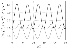
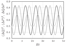
(a)	(b)
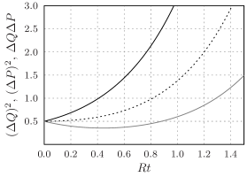
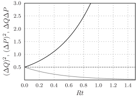
(c)	(d)

Figure 1: Plots of $(\Delta Q)^{2}$ (black), $(\Delta P)^{2}$ (gray) and $\Delta Q\Delta P$ (dotted black) by $Rt$ for $\hbar=\gamma=1$ and (a) $r=2$, $\theta=\frac{\pi}{3}$, $\omega=5$ (plots of (3.21) and (3.22)), (b) $r=2$, $\theta=0$, $\omega=5$ (plots of (3.25) and (3.26)), (c) $r=2$, $\theta=\frac{\pi}{4}$, $\omega=0$ (plots of (3.30) and (3.31)), (d) $r=2$, $\theta=0$, $\omega=0$ (plots of (3.33) and (3.34)).

In what follows we will consider several particular cases of the choice of parameters $\omega,\alpha,\beta,\gamma$. First let us take $\beta=0$ and $\alpha>0$. Then $r=\alpha$ and $\theta=0$. In this case we get that

$$\begin{split}(\Delta Q)^{2}&=\frac{\hbar}{2}\gamma^{-1}\left(1+\frac{\sin^{2}(Rt)}{R}\left(\frac{2r^{2}+(\gamma^{2}-1)\omega^{2}}{R}+2r\cot(Rt)\right)\right),\\ (\Delta P)^{2}&=\frac{\hbar}{2}\gamma\left(1+\frac{\sin^{2}(Rt)}{R}\left(\frac{2r^{2}+(\gamma^{-2}-1)\omega^{2}}{R}-2r\cot(Rt)\right)\right),\end{split}$$ (3.23)

and

$$(\Delta Q)^{2}(\Delta P)^{2}=\frac{\hbar^{2}}{4}\biggl{(} 1+(\gamma^{2}+\gamma^{-2})\frac{2\omega^{2}r^{2}}{R^{4}}\sin^{4}(Rt)+(\gamma^{2}+\gamma^{-2}-2)\frac{\omega^{2}}{R^{2}}\sin^{2}(Rt)$$

$${}-(\gamma^{2}-\gamma^{-2})\frac{2\omega^{2}r}{R^{3}}\sin^{3}(Rt)\cos(Rt)\biggr{)}.$$ (3.24)

If additionally $\gamma=1$ we receive

$$\begin{split}(\Delta Q)^{2}&=\frac{\hbar}{2}\left(1+\frac{2r}{R}\sin^{2}(Rt)\left(\frac{r}{R}+\cot(Rt)\right)\right),\\ (\Delta P)^{2}&=\frac{\hbar}{2}\left(1+\frac{2r}{R}\sin^{2}(Rt)\left(\frac{r}{R}-\cot(Rt)\right)\right),\end{split}$$ (3.25)

and

$$(\Delta Q)^{2}(\Delta P)^{2}=\frac{\hbar^{2}}{4}\left(1+\frac{4\omega^{2}r^{2}}{R^{4}}\sin^{4}(Rt)\right).$$ (3.26)

Now, let us consider the case $\omega^{2}<\alpha^{2}+\beta^{2}$ taking $\omega=0$. Then $R=r$ and

$$\begin{split}Q(q,p,t)&=(q\cos\theta+p\sin\theta)\sinh(rt)+q\cosh(rt),\\ P(q,p,t)&=(q\sin\theta-p\cos\theta)\sinh(rt)+p\cosh(rt).\end{split}$$ (3.27)

Moreover,

$$\begin{split}(\Delta Q)^{2}&=\frac{\hbar}{2}\gamma^{-1}\bigl{(}\cosh(2rt)+\cos\theta\sinh(2rt)+(\gamma^{2}-1)\sin^{2}\theta\sinh^{2}(rt)\bigr{)},\\ (\Delta P)^{2}&=\frac{\hbar}{2}\gamma\bigl{(}\cosh(2rt)-\cos\theta\sinh(2rt)+(\gamma^{-2}-1)\sin^{2}\theta\sinh^{2}(rt)\bigr{)}.\end{split}$$ (3.28)

and

$$(\Delta Q)^{2}(\Delta P)^{2}=\frac{\hbar^{2}}{4}\Bigl{(} 1+\sin^{2}\theta\sinh^{2}(2rt)+(\gamma^{2}-1)\sin^{2}\theta\sinh^{2}(rt)\bigl{(}\cosh(2rt)-\cos\theta\sinh(2rt)\bigr{)}$$

$${}+(\gamma^{-2}-1)\sin^{2}\theta\sinh^{2}(rt)\bigl{(}\cosh(2rt)+\cos\theta\sinh(2rt)\bigr{)}\Bigr{)}.$$ (3.29)

Again, if additionally $\gamma=1$ we get

$$\begin{split}(\Delta Q)^{2}&=\frac{\hbar}{2}\bigl{(}\cosh(2rt)+\cos\theta\sinh(2rt)\bigr{)}=\frac{\hbar}{2}\left(e^{2rt}\cos^{2}\frac{\theta}{2}+e^{-2rt}\sin^{2}\frac{\theta}{2}\right),\\ (\Delta P)^{2}&=\frac{\hbar}{2}\bigl{(}\cosh(2rt)-\cos\theta\sinh(2rt)\bigr{)}=\frac{\hbar}{2}\left(e^{-2rt}\cos^{2}\frac{\theta}{2}+e^{2rt}\sin^{2}\frac{\theta}{2}\right),\end{split}$$ (3.30)

and

$$(\Delta Q)^{2}(\Delta P)^{2}=\frac{\hbar^{2}}{4}\left(1+\sin^{2}\theta\sinh^{2}(2rt)\right).$$ (3.31)

From plot (c) in fig. 1 we can see that for $\theta\neq k\pi$, $k\in\mathbb{Z}$ the state is squeezed only at the beginning of time evolution until a certain value of $t$ is reached. Moreover, as is evident from (3.31) the Heisenberg uncertainty relation is not minimized during the whole time evolution.

Further on, let us take $\omega=0$, $\beta=0$ and $\alpha>0$. Then

$$\begin{split}Q(q,p,t)&=qe^{rt},\\ P(q,p,t)&=pe^{-rt}.\end{split}$$ (3.32)

Moreover,

$$\begin{split}(\Delta Q)^{2}&=\frac{\hbar}{2}\gamma^{-1}e^{2rt},\\ (\Delta P)^{2}&=\frac{\hbar}{2}\gamma e^{-2rt},\end{split}$$ (3.33)

and

$$(\Delta Q)^{2}(\Delta P)^{2}=\frac{\hbar^{2}}{4}.$$ (3.34)

In this case, if $\gamma\leq 1$, the state remains an ideal squeezed state during the whole time evolution.

Finally, let us consider the case $\omega^{2}=\alpha^{2}+\beta^{2}$. In this case

$$\begin{split}(\Delta Q)^{2}&=\frac{\hbar}{2}\left((1+\alpha t)^{2}\gamma^{-1}+(\beta+\omega)^{2}t^{2}\gamma\right),\\ (\Delta P)^{2}&=\frac{\hbar}{2}\left((\beta-\omega)^{2}t^{2}\gamma^{-1}+(1-\alpha t)^{2}\gamma\right),\end{split}$$ (3.35)

and

$$(\Delta Q)^{2}(\Delta P)^{2}=\frac{\hbar^{2}}{4}\bigl{(}1-2\alpha^{2}t^{2}+2\alpha^{4}t^{4}+(1+\alpha t)^{2}(\beta-\omega)^{2}t^{2}\gamma^{-2}+(1-\alpha t)^{2}(\beta+\omega)^{2}t^{2}\gamma^{2}\bigr{)}.$$ (3.36)

It can be seen that during time development the squeezing decreases in time until it is completely destroyed at certain instance of time. Moreover, the Heisenberg uncertainty relation is not minimized during the whole time evolution.

Note, that after performing the following transformation to new coordinates (rotation by angle $\frac{\theta}{2}$)

$$\begin{split}q^{\prime}&=q\cos\frac{\theta}{2}+p\sin\frac{\theta}{2},\\ p^{\prime}&=-q\sin\frac{\theta}{2}+p\cos\frac{\theta}{2}\end{split}$$ (3.37)

the Hamiltonian $H(q,p)$ (3.11) transforms into

$$H(q^{\prime},p^{\prime})=\frac{1}{2}\omega(p^{\prime 2}+q^{\prime 2})+rq^{\prime}p^{\prime}.$$ (3.38)

Thus, we can always perform the reduction to the case $\beta=0$ and $\alpha>0$ provided that we will be working with rotated variables $q^{\prime},p^{\prime}$. Furthermore, in a case $\omega^{2}>\alpha^{2}+\beta^{2}$ the following one-parameter family of linear canonical transformations of coordinates

$$\begin{split}q^{\prime}&=\frac{Ra+\alpha A}{\omega+\beta}q+Ap,\\ p^{\prime}&=\frac{\alpha a-RA}{\omega+\beta}q+ap,\end{split}\quad A=\pm\sqrt{\frac{\omega+\beta}{R}-a^{2}},\quad a\in\mathbb{R}$$ (3.39)

transforms the Hamiltonian (3.11) into the following Hamiltonian of the harmonic oscillator with positive frequency

$$H(q^{\prime},p^{\prime})=\frac{1}{2}R(p^{\prime 2}+q^{\prime 2}),$$ (3.40)

and the one-parameter family of transformations

$$\begin{split}q^{\prime}&=-\frac{Ra+\alpha A}{\omega+\beta}q-Ap,\\ p^{\prime}&=\frac{\alpha a-RA}{\omega+\beta}q+ap,\end{split}\quad A=\pm\sqrt{-\frac{\omega+\beta}{R}-a^{2}},\quad a\in\mathbb{R}$$ (3.41)

leads to the following Hamiltonian of the harmonic oscillator with negative frequency

$$H(q^{\prime},p^{\prime})=-\frac{1}{2}R(p^{\prime 2}+q^{\prime 2}).$$ (3.42)

On the other hand, in a case $\omega^{2}<\alpha^{2}+\beta^{2}$ the following one-parameter family of linear canonical transformations of coordinates

$$\begin{split}q^{\prime}&=-\frac{R+\alpha}{\omega+\beta}aq-ap,\\ p^{\prime}&=\frac{R-\alpha}{2Ra}q-\frac{\omega+\beta}{2Ra}p,\end{split}\quad a\in\mathbb{R}$$ (3.43)

transforms the Hamiltonian (3.11) into the following Hamiltonian

$$H(q^{\prime},p^{\prime})=Rq^{\prime}p^{\prime},$$ (3.44)

and the one-parameter family of transformations

$$\begin{split}q^{\prime}&=\frac{R-\alpha}{\omega+\beta}aq-ap,\\ p^{\prime}&=\frac{R+\alpha}{2Ra}q+\frac{\omega+\beta}{2Ra}p,\end{split}\quad a\in\mathbb{R}$$ (3.45)

leads to the following Hamiltonian

$$H(q^{\prime},p^{\prime})=-Rq^{\prime}p^{\prime}.$$ (3.46)

Summarizing the above considerations we conclude that when $\omega^{2}>\alpha^{2}+\beta^{2}$ we can always reduce the dynamics to the harmonic oscillator, and when $\omega^{2}<\alpha^{2}+\beta^{2}$ we can reduce the dynamics to the case $\omega=\beta=0$, provided that we will be working with new variables $q^{\prime},p^{\prime}$. In the frame of original variables $q,p$ it means that for the considered system there always exist canonically conjugated observables $q^{\prime}=q^{\prime}(q,p),p^{\prime}=p^{\prime}(q,p)$ which preserve the minimal uncertainty during time evolution.

4 Hamiltonian system with purely quantum time evolution

Let us consider a system described by a Hamiltonian

$$H(q,p)=\lambda q^{2}p^{2},$$ (4.1)

where $\lambda$ is a characteristic constant of the system. By a coherent state of such system we will call a state for which uncertainties of position and momentum satisfy (3.4). Coherent states are of the form of Gaussian functions

$$\rho(q,p)=2\exp\left(-\frac{(q-q_{0})^{2}}{\hbar\alpha}\right)\exp\left(-\frac{(p-p_{0})^{2}}{\hbar\alpha^{-1}}\right),$$ (4.2)

where $(q_{0},p_{0})$ is a mean position and momentum in the state $\rho$, and are parametrized by $\alpha>0$.

The solution of the quantum Hamilton equations (2.9) for the Hamiltonian (4.1) reads [17]

$$\begin{split}Q(q,p,t)&=\sec^{2}(\hbar\lambda t)q\exp\left(\frac{2}{\hbar}\tan(\hbar\lambda t)qp\right),\\ P(q,p,t)&=\sec^{2}(\hbar\lambda t)p\exp\left(-\frac{2}{\hbar}\tan(\hbar\lambda t)qp\right).\end{split}$$ (4.3)

It is well defined for $t\in\mathbb{R}\setminus\{\frac{\pi n}{2\hbar\lambda}\mid n=\pm 1,\pm 2,\dotsc\}$. Note, that this solution differs from the classical one

$$Q_{C}(q,p,t)=qe^{2\lambda tqp},\quad P_{C}(q,p,t)=pe^{-2\lambda tqp},$$ (4.4)

which can be obtained from (4.3) in the limit $\hbar\to 0$. In other words quantum trajectories differ from classical ones. Moreover, time development of position and momentum observables is not well defined for all values of the evolution parameter $t$, contrary to the classical case.

Through direct integration we can calculate the expectation values of $Q$ and $P$ from (4.3) in a coherent state (4.2). The result after introducing

$$\begin{split}a(t)&=\frac{\cos(\hbar\lambda t)}{\sqrt{\cos(2\hbar\lambda t)}}q_{0}+\frac{\alpha\sin(\hbar\lambda t)}{\sqrt{\cos(2\hbar\lambda t)}}p_{0},\\ b(t)&=-\frac{\alpha^{-1}\sin(\hbar\lambda t)}{\sqrt{\cos(2\hbar\lambda t)}}q_{0}+\frac{\cos(\hbar\lambda t)}{\sqrt{\cos(2\hbar\lambda t)}}p_{0},\end{split}$$ (4.5)

reads

$$\begin{split}\langle{Q}\rangle_{\rho}&=\frac{a(t)}{\cos(2\hbar\lambda t)}\exp\biggl{(}\frac{1}{\hbar\alpha}\left(a^{2}(t)-q_{0}^{2}\right)\biggr{)},\\ \langle{P}\rangle_{\rho}&=\frac{b(t)}{\cos(2\hbar\lambda t)}\exp\biggl{(}\frac{\alpha}{\hbar}\left(b^{2}(t)-p_{0}^{2}\right)\biggr{)}.\end{split}$$ (4.6)

Note, that $\langle{Q}\rangle_{\rho}$ and $\langle{P}\rangle_{\rho}$ are well defined only on intervals $(-\frac{1}{4}+n)\frac{\pi}{\hbar\lambda}<t<(\frac{1}{4}+n)\frac{\pi}{\hbar\lambda}$, $n\in\mathbb{Z}$. This once again shows that time evolution of the considered system is not defined for all values of the evolution parameter $t$ and even time development of quantities measured in experiment like expectation values of position and momentum is only well defined on certain intervals of $t$. Observe also, that time evolution of expectation values of $Q$ and $P$ in a coherent state does not coincide with quantum trajectories, as was the case for linear quantum systems.

Let us calculate standard deviations of $Q$ and $P$ in the coherent state $\rho$. To do this first we need to calculate expectation values of $Q^{2}=Q\star_{M}Q$ and $P^{2}=P\star_{M}P$. To calculate $Q^{2}$ we can perform Wick rotation $t\to i\tau$ and use the integral formula (2.3) for the Moyal product. We find that

$$(Q\star_{M}Q)(q,p,t)=\sec^{3}(2\hbar\lambda t)q^{2}\exp\left(\frac{2}{\hbar}\tan(2\hbar\lambda t)qp\right).$$ (4.7)

Similarly we calculate $P^{2}$

$$(P\star_{M}P)(q,p,t)=\sec^{3}(2\hbar\lambda t)p^{2}\exp\left(-\frac{2}{\hbar}\tan(2\hbar\lambda t)qp\right).$$ (4.8)

The expectation values of $Q^{2}$ and $P^{2}$ can be calculated similarly as $\langle{Q}\rangle_{\rho}$ and $\langle{P}\rangle_{\rho}$. We get the following formulas

$$\begin{split}\langle{Q^{2}}\rangle_{\rho}&=\bigl{(}\cos(4\hbar\lambda t)\bigr{)}^{-3/2}\left(\frac{\hbar}{2}\alpha+a^{2}(2t)\right)\exp\biggl{(}\frac{1}{\hbar\alpha}\left(a^{2}(2t)-q_{0}^{2}\right)\biggr{)},\\ \langle{P^{2}}\rangle_{\rho}&=\bigl{(}\cos(4\hbar\lambda t)\bigr{)}^{-3/2}\left(\frac{\hbar}{2}\alpha^{-1}+b^{2}(2t)\right)\exp\biggl{(}\frac{\alpha}{\hbar}\left(b^{2}(2t)-p_{0}^{2}\right)\biggr{)},\end{split}$$ (4.9)

which are well defined for $(-\frac{1}{4}+n)\frac{\pi}{2\hbar\lambda}<t<(\frac{1}{4}+n)\frac{\pi}{2\hbar\lambda}$, $n\in\mathbb{Z}$.

The standard deviations of $Q$ and $P$ are equal

$$\begin{split}(\Delta Q)^{2}&=\bigl{(}\cos(4\hbar\lambda t)\bigr{)}^{-3/2}\left(\frac{\hbar}{2}\alpha+a^{2}(2t)\right)\exp\biggl{(}\frac{1}{\hbar\alpha}\left(a^{2}(2t)-q_{0}^{2}\right)\biggr{)}-\frac{a^{2}(t)}{\cos^{2}(2\hbar\lambda t)}\exp\biggl{(}\frac{2}{\hbar\alpha}\left(a^{2}(t)-q_{0}^{2}\right)\biggr{)},\\ (\Delta P)^{2}&=\bigl{(}\cos(4\hbar\lambda t)\bigr{)}^{-3/2}\left(\frac{\hbar}{2}\alpha^{-1}+b^{2}(2t)\right)\exp\biggl{(}\frac{\alpha}{\hbar}\left(b^{2}(2t)-p_{0}^{2}\right)\biggr{)}-\frac{b^{2}(t)}{\cos^{2}(2\hbar\lambda t)}\exp\biggl{(}\frac{2\alpha}{\hbar}\left(b^{2}(t)-p_{0}^{2}\right)\biggr{)}\end{split}$$ (4.10)

and are well defined for $(-\frac{1}{8}+n)\frac{\pi}{\hbar\lambda}<t<(\frac{1}{8}+n)\frac{\pi}{\hbar\lambda}$, $n\in\mathbb{Z}$.

Note, that there are no values of the parameters $q_{0},p_{0},\alpha$ such that $(\Delta Q)^{2}(\Delta P)^{2}$ is equal $\frac{\hbar^{2}}{4}$ for all $t$. In other words the coherent state $\rho$ does not remain coherent during time development. It happens to be coherent only for $t=\frac{\pi n}{\hbar\lambda}$, $n\in\mathbb{Z}$. Moreover, the state $\rho$ is not getting squeezed during time evolution in the sense that $(\Delta Q)^{2}$ or $(\Delta P)^{2}$ is not getting smaller than its initial value. In fig. 2 are presented plots of $(\Delta Q)^{2}$ and $(\Delta P)^{2}$ for certain values of parameters $\lambda,\alpha,q_{0},p_{0}$.

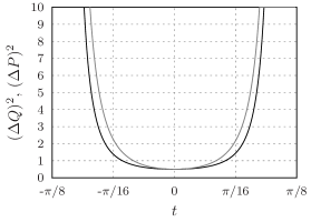
Figure 2: Plots of $(\Delta Q)^{2}$ (black) and $(\Delta P)^{2}$ (gray) by $t$ given by equation (4.10) for $\hbar=\lambda=\alpha=1$, $q_{0}=0.01$, $p_{0}=1$.

5 Conclusions and final remarks

In the paper we have investigated the behavior of coherent and squeezed states during time development generated by two distinct Hamiltonians. As the first Hamiltonian we took a Hamiltonian quadratic in phase space variables $q,p$. This was one of the simplest Hamiltonians for which classical and quantum flows coincided, and even in this case the initial squeezed state remained squeezed only on certain intervals of $t$, and only for certain values of $t$ the state was coherent. In fact, only for particular choice of parameters we get the preservation of coherence and squeezing during the whole time evolution. This result allows to suspect that for more general Hamiltonians the coherence and squeezing of states will rarely appear during time development. Furthermore, we showed that after performing appropriate linear canonical transformation of phase space coordinates we could always transform the Hamiltonian quadratic in phase space variables to a Hamiltonian for which the coherence and squeezing will be preserved during time development, provided that the coherence and squeezing will be defined with respect to the transformed phase space coordinates.

As the second example we considered the simplest Hamiltonian with purely quantum time evolution. In this case the coherence was destroyed during time development and squeezing did not appear. Moreover, the quantum trajectories and expectation values of observables of position and momentum were well defined only on certain intervals of $t$, which raises problems and questions of interpretation of such kind of time evolution. This could suggest that the Moyal quantization (Weyl quantization in position representation) applied for the system (4.1) is not the proper quantization for such system, and that one should use some other quantization in which at least expectation values of observables of position and momentum will be well defined for all values of $t$. Another question is whether in considered quantization there are some quantum states in which these expectation values are properly defined for all $t$ (states (4.2) does not have such property). We can suspect that for more general quantum systems even more peculiarities can appear, which is an interesting topic for further investigation.

References

Glauber [1963]R. J. Glauber, Phys.
Rev. 131, 2766 (1963).
Glauber [1964]R. J. Glauber, in Quantum Optics
and Electronics, edited by C. DeWitt, A. Blandin, and C. Cohen-Tannoudji (Gordon and
Breach, New York, 1964) pp. 63–185.
Sudarshan [1963]E. C. G. Sudarshan, Phys. Rev. Lett. 10, 277 (1963).
Walls [1983]D. Walls, Nature 306, 141
(1983).
Han et al. [1988]D. Han, Y. S. Kim, and M. E. Noz, Phys. Rev. A 37, 807 (1988).
Hillery et al. [1984]M. Hillery, R. F. O’Connell, M. O. Scully, and E. P. Wigner, Phys.
Rep. 106, 122 (1984).
Groenewold [1946]H. J. Groenewold, Physica (Utrecht) 12, 405 (1946).
Moyal [1949]J. E. Moyal, Proc.
Cambridge Philos. Soc. 45, 99 (1949).
Bayen et al. [1977]F. Bayen, M. Flato,
C. Frønsdal, A. Lichnerowicz, and D. Sternheimer, Lett. Math. Phys. 1, 521 (1975–1977).
Bayen et al. [1978a]F. Bayen, M. Flato,
C. Frønsdal, A. Lichnerowicz, and D. Sternheimer, Ann. Phys. 111, 61 (1978a).
Bayen et al. [1978b]F. Bayen, M. Flato,
C. Frønsdal, A. Lichnerowicz, and D. Sternheimer, Ann. Phys. 111, 111 (1978b).
Błaszak and Domański [2012a]M. Błaszak and Z. Domański, Ann. Phys. 327, 167
(2012a), arXiv:1009.0150 [math-ph]
.
Baker [1958]G. A. Baker, Jr., Phys. Rev. 109, 2198 (1958).
Błaszak and Domański [2013]M. Błaszak and Z. Domański, Ann. Phys. 339, 89
(2013), arXiv:1305.4518 [math-ph] .
Wigner [1932]E. P. Wigner, Phys.
Rev. 40, 749 (1932).
Błaszak and Domański [2012b]M. Błaszak and Z. Domański, Phys. Lett. A 376, 3593
(2012b), arXiv:1208.0720 [math-ph]
.
Dias and Prata [2007]N. C. Dias and J. N. Prata, J.
Math. Phys. 48, 012109
(2007), arXiv:quant-ph/0604167v1
.