Semiconductor of spinons: from Ising band insulator to orthogonal band insulator

Abstract

Within the ionic Hubbard model, electron correlations transmute the single-particle gap of a band insulator into a Mott gap in the strong correlation limit. However understanding the nature of possible phases in between these two extreme insulating phases remains an outstanding challenge. We find two strongly correlated insulating phases in between the above extremes: (i) The insulating phase just before the Mott phase can be viewed as gapping a non-Fermi liquid state of spinons through staggered ionic potential. The quasi-particles of underlying spinons are orthogonal to physical electrons and hence they do not couple to photoemission probes, giving rise to ”ARPES-dark” state due to which the ARPES gap will be larger than optical and thermal gap. (ii) The correlated insulating phase just after the normal band insulator corresponds to the ordered phase of slave Ising spins (Ising insulator) where charge configuration is controlled by an underlying Ising variable which indirectly couples to external magnetic field and hence gives rise to additional temperature and field dependence in semiconducting properties. In the absence of tunability for the Hubbard $U$, such a temperature and field dependence can be conveniently employed to achieve further control on the transport properties of Ising-based semiconductors. The rare earth monochalcogenide semiconductors where the magneto-resistance is anomalously large can be a candidate system for the ordered phase of Ising variable where pairs of charge bosons are condensed in the background. Combining present results with our previous dynamical mean field theory study, we argue that the present picture holds if the ionic potential is strong enough to survive the downward renormalization of the ionic potential caused by Hubbard $U$.

I INTRODUCTION

Electron conduction in periodic structures can cease for two reasons. The simplest is to couple single-particle states across a reduced Brillouin zone by an off-diagonal matrix elements due to reduction in the periodicity. However the second and more exciting way is to introduce strong electron correlations where due to Coulomb interactions, as suggested by N. Mott, electron conduction in an otherwise conducting state is interrupted MottBook . This may seem to suggest that strong correlation has its most dramatic effect on metals by transforming them into many-body Mott insulators. The canonical model within which the metal-to-insulator transition (MIT) problem is investigated is the Hubbard model Fujimori . Efforts to understand the nature of MIT has lead to many technical Gutzwiller ; MuthukumarGros ; Metzner ; Senechal ; Adibi ; Vladimir ; OvchinikovBook ; Sorella ; Imada ; Kotliar ; Tohyama ; Dagotto and conceptual LeeWenNagaosa ; Florens2004 ; Sigrist ; HasanSlaveSpin ; Zaanen developments providing clues into possible mechanisms of non-Fermi liquid formation.

But even more challenging question is what happens when both mechanisms of gap formation are simultaneously present, i.e. what are the properties of strongly correlated band insulators or semiconductors? Let us formalize the problem as follows: Imagine a staggered potential of strength $\Delta$ (the ionic potential) that can gap out the parent metallic state and sets the scale of the single-particle gap. When the Hubbard interaction $U$ is turned on in such an already gapped state (band insulator) an interesting competition between the Hubbard $U$ and the staggered potential $\Delta$ sets in. This is the simplest model addressing the competition between a ”many-body” gap parameter $U$ and a ”single-particle” gap parameter $\Delta$ which is called ionic Hubbard model Egami . The band insulating state at $U=0$ is adiabatically connected to the insulating state at non-zero but small values of $U\ll\Delta$ as the effect of weak Hubbard $U$ is to renormalize the parent metallic state on top of which the ionic potential creates a band insulator (BI) state. In the opposite limit of strong correlations $U\gg\Delta$ one gets a Mott insulating (MI) state. Although these two extreme limits both represent insulating states, the origin of gap in the former case is a simple one-particle scattering, while in the later case the gap has a many-body character arising from projection of doubly occupied configurations.

The nature of possible state(s) between the above two extreme insulating states has been the subject of debates in the past decade. In one dimension Fabrizio and coworkers Fabrizio find an ordered state. In two dimensions Hafez-Torbati and coworkers find orientational and bond ordering phase in between the Mott and band insulators Hafez2015 . The topologically non-trivial variant of the model was considered by Prychynenko and coworkers Huber who find for topologically trivial situation two spin density wave states are sandwiched between the band and Mott insulating states. In the limit of infinite dimensions however, Garg and coworkers using the dynamical mean field theory found that the competition between the tendency of the ionic potential $\Delta$ and the Hubbard term $U$ gives rise to a metallic state Garg . Within a perturbative continuous unitary transformation one finds a metallic state when the Hubbard $U$ and the ionic potential $\Delta$ are comparable Hafez2009 . Similar result were obtained in two dimensions Baudim . The method of dynamical mean field theory was also applied to study the quantum phase transitions of the ionic Hubbard model on the honeycomb lattice. Starting from massive Dirac fermions on the honeycomb lattice the competition between $U$ and the single-particle gap parameter $\Delta$ (known as mass term when it comes to Dirac fermions) gives rise to massless Dirac fermions Ebrahimkhas . A recent strong coupling expansion gives a quantum critical semi-metallic state Adibi .

When electron correlations in a conductor are not strong enough to transform the metallic state to a Mott insulator, they give rise to possible non-Fermi liquid states. From this point of view one may now turn on the ionic potential $\Delta$ and ask the following question: How does this staggered potential interfere with possible non-Fermi liquid state of the parent metal? Can the ionic potential gap out a non-Fermi liquid state? With this motivation, let us summarize one of the simplest mechanisms of creating a non-Fermi liquid state, and then add the ionic potential $\Delta$ to it in a self-consistent way. This is the question on which we will be focused in this paper.

Recently Nandkishore and coworkers have argued that starting from a metallic state, as one increases the Hubbard $U$ beyond $U_{\perp}$ the Fermi liquid (FL) undergoes a phase transition to an exotic non-FL state termed orthogonal metal (OM). Upon further increase in the interaction strength beyond $U_{c}$ the system becomes a Mott insulator OMPhys ; Nandkishore . OM is an interesting – and perhaps the simplest – non-FL state for $U_{\perp}<U<U_{\rm Mott}$ that separates a FL from a Mott insulator. In the FL phase the rotor variable is ordered, i.e. the phase variable has small fluctuations meaning that the electric charge has large fluctuations. When the rotor variable disorders, earlier interpretation would assume that wild fluctuations of the rotor field that is responsible for vanishing of the rotor variable corresponds to freezing of charge fluctuations and hence making the system a Mott insulator Florens2004 . However, Nandkishore and coworkers argued that even if the rotor variable is disordered, i.e. $\langle e^{i\theta}\rangle=0$ for $U>U_{b}$ meaning that the single boson $b\sim e^{i\theta}$ is not condensed, a two-boson combination can still be condensed, $\langle bb\rangle\neq 0$. This gives a new chance to charge fluctuations to survive in the form of an Ising variable which then can be naturally captured within a slave spin approach Sigrist where the condensation of two-boson combination is reflected in a non-zero Ising order parameter for $U_{b}<U<U_{\perp}$. This phase can be dubbed Ising metal. The disordered phase of such an Ising variable for $U_{\perp}<U<U_{\rm Mott}$ will correspond to OM state where although quasiparticle weight corresponding to physical electrons is zero, its transport behaviour is metallic. To see this, the following simple and powerful argument is due to Nandkishore and coworkers: Within the slave spin representation the physical electron is represented as $c^{\dagger}_{\sigma}=f^{\dagger}_{\sigma}\tau^{x}$. The $U(1)$ transformation representing the conservation of the electric (Noether) charge can only be incorporated into the spinon $f^{\dagger}_{\sigma}$, simply because the Pauli matrix $\tau^{x}$ is purely real. Therefore the $f$ spinon inherits the whole charge from the parent electron and after the Ising disordering transition at $U_{\perp}$ the spinons will continue to display metallic transport properties despite that the quasiparticle weight of the physical electrons has been already lost at $U_{\perp}$ as it is proportional to Ising magnetization Nandkishore . If instead of a metallic state at $U=0$, one starts with a semi-metallic state (such as graphene) the state corresponding to disordering transition Ising pseudo-spins will be an orthogonal semi-metal Chinese . For our purpose in the present paper, we would like to see that, both the orthogonal metal phase for $U_{\perp}<U<U_{\rm Mott}$ and the Ising metal (IM) for $U_{b}<U<U_{\perp}$ are equally interesting when one gaps out the underlying metallic state.

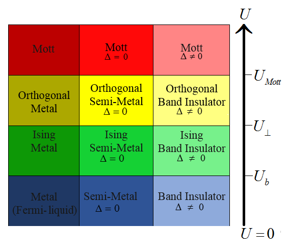
Figure 1: (Color online) The schematic representation of the effect of correlation on three starting states. The non-interacting state from which we start is drawn in the bottom row. Left column corresponds to metallic state, middle column stands for semi-metallic state and the right column denotes the band insulating state. All columns at very large $U$ end in the Mott insulating states (top row). The middle row is the corresponding ”orthogonal” phase where the transport is controlled by the spinons that inherit the charge of the original electrons.

Now let us turn on the ionic potential $\Delta$ that locally couples to the electric charge as $(-1)^{i}\Delta c^{\dagger}_{i\sigma}c_{i\sigma}$ at every site $i$ of the lattice. The Ising term $\tau^{x}$ is ”eaten up” by the $U(1)$ invariance of this term and the spinon density directly couple to the ionic potential as $(-1)^{i}\Delta f^{\dagger}_{i\sigma}f_{i\sigma}$. This is because spinons carry the whole charge and hence their density couples to external electrostatic potential (including even random potentials). The above term clearly gaps out both the IM and the OM conducting state of spinons and creates a band insulator of Ising metal and spinon metal. These phases can be called Ising band insulator (IBI) and orthogonal band insulator (OBI), respectively as they are born out of an underlying IM and OM states. When the (thermal) gap of the OBI is small enough to comply with semiconducting gaps we will have an orthogonal semiconductor, i.e. a semiconductor of spinons that has been separated from an Ising semiconductor.

Our discussion is schematically summarized in Fig. 1 where the notion of Ising and orthogonal state before a Mott state has been illustrated for three weak coupling states: metal, semimetal, and band insulator. The weak coupling states at the bottom row (blue) turn into their Ising counterpart (green) by increasing $U$ beyond $U_{b}$ where at which the single boson condensate (rotor order parameter) vanishes. In the Ising (green) phase, still the physical electrons are governing the transport properties, but the charge condensate is survived as an Ising order which eventually vanishes at $U_{\perp}$. From this point the orthogonal (yellow) phase starts. By further increasing the Hubbard $U$ beyond $U_{\rm Mott}$ even the residual interaction between the spinons of the orthogonal phase become so strong that renders the system Mott insulating.

Therefore the intuitive picture that emerges for the ionic Hubbard model (right column) is as follows: At small values of Hubbard $U$ (blue region) the gapped state is adiabatically connected to a band insulator. When $U$ crosses $U_{b}$ at which the single bosons ”quantum evaporate” from the condensate but the boson pairs form a condensate, we will have IBI where the charge variable is Ising-like and its characteristic Ising-like properties is expected to give rise to unusual semiconducting properties (green region). By further increasing $U$ up to $U_{\perp}$ where the Ising order parameter of IBI vanishes, the OBI phase (yellow region) starts which is eventually gapped by prohibition of doubly occupancy at $U_{\rm Mott}$.

In the OBI phase for $U_{\perp}<U<U_{\rm Mott}$ (yellow region) the disordering of the underlying slaved Ising variables leaves the states in bottom of conduction and top of valence bands inaccessible to ARPES, while accessible to any probe coupling to the electric current (charge), such as optical conductivity, cyclotron resonance and thermal probes. This plays a significant role in experimental discrimination of the orthogonal insulators (semiconductors) from their Ising (green) or normal (blue) relatives. The bandwidth and hence the effective mass of the correlated semiconducting phase IBI is controlled by Ising order parameter which will then possess Ising-like temperature dependencies and hence e.g. cyclotron frequency will acquire Ising-like temperature dependence, etc; while the OBI phase is characterized by wider ARPES gap compared to thermal gap.

The results of this paper apply to a quite general correlated insulators on any two-dimensional lattice. However in this paper we focus on honeycomb system where the parent band insulator is described by massive Dirac electrons GappedEpitaxialGraphene . At the end we contrast the above possibilities with our previous dynamical mean field study of the ionic Hubbard model on honeycomb lattice Ebrahimkhas to discuss plethora of Ising and orthogonal phases that maybe conducting or insulating. This will shed a new light: To get a chance to realize IBI the ionic potential $\Delta$ must be large enough. To realize OBI, the ionic potential must be even larger than what is required to realize IBI. For very small values of $\Delta$, only the Ising and orthogonal phase of massless Dirac fermions can be realized which corresponds to a orthogonal semi-metal.

This paper is organized as follows: In section II after introducing the ionic Hubbard model, we review the slave-rotor method and customize it for the ionic Hubbard model. In section III we adopt the version of slave-spin method employed in Sigrist . Based on symmetry principles we discuss under what circumstances the Lagrange multiplier implementing the constraint between Ising pseudo-spin and spinon degrees of freedom vanishes. In section IV we discuss the results and summarize the findings at the end.

II Ionic Hubbard model and slave rotor method

We are interested in the phase diagram of the Hubbard model augmented by a staggered ionic potential of strength $\Delta$ as follows:

$$H=H_{0}+\frac{U}{2}\sum_{i}(n_{i\uparrow}+n_{i\downarrow}-1)^{2}$$ (1)

$$H_{0}=-t\sum_{\langle i,j\rangle\sigma}c^{\dagger}_{i\sigma}c_{j\sigma}+\Delta\sum_{i\sigma}(-1)^{i}n_{i\sigma}-\mu\sum_{i\sigma}n_{i\sigma}$$ (2)

where $c^{\dagger}_{i\sigma}$ creates an electron at a localized orbital in site $i$ with spin $\sigma$, $n_{i\sigma}=c^{\dagger}_{i\sigma}c_{i\sigma}$ is the occupation number, $U$ is the on-site Hubbard repulsion, $t$ is the hopping amplitude which will be set as the unit of energy through out the paper, $\Delta$ is the ionic potential, and $\mu$ is the chemical potential that at half-filling in the present representation turns out to be $\mu=0$.

II.1 Slave rotor method

The slave rotor formulation is one of the slave particle family methods employed in studying the Hubbard model that provides a very economical representation of the charge state of an orbital in terms of a rotor variable conjugate to an angular momentum operator locked to the charge Florens2004 . This method can also be applied to the study of Anderson impurity problem Florens2002 . In this approach the local Hilbert space is represented by a direct product of the Hilbert space of a fermion carrying the spin index (the so called spinon) and a rotor that controls the charge state of the system as $\left|\psi\right\rangle=\left|{{\psi}_{f}}\right\rangle\left|{{\psi}_{\theta}}\right\rangle$. In terms of operator creating a particle from its vacuum the above equation can be represented as,

$$\hat{c}_{i\sigma}^{\dagger}=f_{i\sigma}^{\dagger}{{e}^{-i{{\theta}_{i}}}},$$ (3)

where $f^{\dagger}_{i\sigma}$ is the spinon creation operator and $\theta_{i}$ is the rotor variable at site $i$. The physical Hilbert space of the electron in terms of the spinons and rotors is constructed from the following states:

$$\left|0\right\rangle\equiv\left|0\right\rangle_{f}\left|-1\right\rangle_{\theta}$$

$$\left|\uparrow\right\rangle\equiv\left|\uparrow\right\rangle_{f}\left|0\right\rangle_{\theta}$$

$$\left|\downarrow\right\rangle\equiv\left|\downarrow\right\rangle_{f}\left|0\right\rangle_{\theta}$$

$$\left|\uparrow\downarrow\right\rangle\equiv\left|\uparrow\downarrow\right\rangle_{f}\left|1\right\rangle_{\theta}$$ (4)

where $|\rangle_{\theta}$ represents a state in the rotor space, and $|\rangle_{f}$ represents states in the spinon Hilbert space. As can be seen in the above representation, state such as $|\uparrow\rangle_{f}|-1\rangle_{\theta}$ containing one $\uparrow$-spin spinon and corresponding to angular momentum eigen state of $-1$ does not correspond to any physical state. Such redundancy is a characteristic of auxiliary particle methods where the physical Hilbert space is enormously enlarge. What we gain in the enlarged Hilbert space is the gauge freedom. But the physically sensible states are obtained from those in the enlarged space by projecting them to the physical space. In the present case such a projection amounts to the constraint,

$$\sum\limits_{\sigma}{f_{i\sigma}^{\dagger}{{f}_{i\sigma}}}=L_{i}+1$$ (5)

that locks the particle number to angular momentum. It can be seen that all of the states in Eq. (4) satisfy this constraint. If the above constraint can be implemented exactly, then either of the representation in terms of original electrons or in terms of spinons and rotors will describe the same physics. But the full-fledged implementation of the above projection requires to take a complete care of the fluctuations of the internal gauge fiedls that glue spinons and rotor fields. In the present work we treat the constraint in the mean field via a space- and time-independent Lagrange multiplier. This is known as the slave rotor mean field approximation Florens2004 ; Paramekanti .

Let us proceed with representing the electron operators in terms of spinons and rotors, Eq.(3),

$$H=-\sum\limits_{\left\langle ij\right\rangle,\sigma}{f_{i\sigma}^{\dagger}{{f}_{j\sigma}}{{e}^{-i{{\theta}_{ij}}}}+{\rm h.c.}}+\Delta\sum\limits_{i}{f_{i}^{\dagger}{{f}_{i}}}-\Delta\sum\limits_{j}{f_{j}^{\dagger}{{f}_{j}}}$$

$$+\frac{U}{2}\sum\limits_{i}{L_{i}^{2}-\mu\sum\limits_{i\sigma}{f_{i\sigma}^{\dagger}{{f}_{i\sigma}}}}+\lambda\sum_{i}\left(f^{\dagger}_{i\sigma}f_{i\sigma}-L-1\right),$$ (6)

where the hopping amplitude $t$ of original electrons is set as the unit of energy, $t=1$, $\theta_{ij}=\theta_{i}-\theta_{j}$, the Hubbard term of Eq. (1) has been transformed with the aid of the constraint (5), $\mu$ is the chemical potential that becomes zero at half-filling which is our focus in this paper, and $\lambda$ is a position-independent Lagrange multiplier that implements the constraint (5) on average. The merit of representation in terms of auxiliary rotor variables is that the quartic interaction between the fermions $U/2{{\sum\nolimits_{i\sigma}{\left(n_{i\sigma}-1\right)}}^{2}}$ is replaced by a simple rotor kinetic energy $U{{L}^{2}}/2$ at every site, where the angular momentum $L=-i{{\partial}_{\theta}}$ is a variable that is associated with a $O(2)$ quantum rotor $\theta$.

Apart from the kinetic term that involves spinons and rotors on neighbouring sites, the above Hamiltonian is decoupled into rotor ($\theta$-only), and spinon ($f$-only) terms. As for the first term we introduce mean field variables,

$$\chi_{\theta}=\left\langle e^{i\theta_{i}}e^{-i\theta_{j}}\right\rangle_{\theta},$$ (7)

$$\chi_{f}=\left\langle\sum\nolimits_{\sigma}f_{\sigma i}^{\dagger}{f}_{\sigma j}\right\rangle_{f},$$ (8)

to decouple the kinetic term, which eventually gives decoupled rotor, $H_{\theta}$ and spinon $H_{f}$ Hamiltonians,

$$H_{f}=-\sum\limits_{\langle ij\rangle,\sigma}f_{i\sigma}^{\dagger}f_{j\sigma}\chi_{\theta}+{\rm h.c}+(\lambda-\mu)\sum_{j\sigma}f^{\dagger}_{j\sigma}f_{j\sigma}$$

$$+\Delta\sum_{i\in A}f_{i\sigma}^{\dagger}f_{i\sigma}-\Delta\sum_{j\in B}f_{j\sigma}^{\dagger}f_{j\sigma},$$ (9)

and

$$H_{\theta}=\sum_{\langle i,j\rangle}\chi_{f}e^{i\theta_{i}-i\theta_{j}}+h.c.+\sum_{j}\left(\frac{U}{2}L_{j}^{2}-\lambda L_{j}\right),$$ (10)

where $A$ and $B$ are the two sub-lattices on the honeycomb lattice. In the above equation, solution of the $H_{f}$ requires a knowledge of $\chi_{\theta}$ which according to Eq. (7) can only be calculated after having diagonalized the rotor sector $H_{\theta}$. The later itself depends on unknown quantity $\chi_{f}$ that according to Eq. (8) can be obtained from the $H_{f}$ Hamiltonian. This provides a self-consistency loop, i.e. the rotor and the spinon sectors talk to each other via the mean-field self-consistency equations, (7) and (8).

It is interesting to note that in Eq. (9) the ionic potential $\Delta$, being a local potential couples only to the spinon density. This considerably simplifies the analysis of the problem. Indeed in the absence of ionic potential $\Delta$, the spinon sector would have been described by spinon hopping Hamiltonian with renormalized hopping amplitudes whose reduced kinetic energy is encoded in $\chi_{\theta}$ which is self-consistently determined by the rotor sector. When the ionic potential is turned on, the spinon sector describes spinons hopping with renormalized hopping parameters $\chi_{\theta}$, plus an additional Bragg reflection due to doubling of the unit cell that always gaps out the spinon sector and the spectrum in the spinon-sector becomes,

$$\varepsilon_{f}(\vec{k})=\pm\sqrt{\chi_{\theta}^{2}|\phi(\vec{k})|^{2}+\Delta^{2}}$$ (11)

where $\phi(\vec{k})=1+e^{i\vec{k}.\vec{a}_{1}}+e^{i\vec{k}.\vec{a}_{2}}$ with $\vec{a}_{1}$ and $\vec{a}_{2}$ unit being translation vectors of the honeycomb lattice.

Now let us turn to determination of chemical potential $\mu$ and Lagrange multiplier field $\lambda$. Since we are interested in the competition between $U$ and $\Delta$, we stay at half-filling where even in the $U=0$ limit the system is described by a simple band insulator. The particle-hole symmetry of the original Hamiltonian in terms of physical electrons simply implies that at half-filling $\mu=0$. Since we want to fix the average occupation at $n=1$, the constraint (5) implies that on average one should have $\langle L_{j}\rangle=0$ for every lattice site $j$. Now imagine that in a rotor Hilbert space corresponding to a given total angular momentum $\ell$, we construct the local angular momentum operator $UL_{j}^{2}/2-\lambda L_{j}$ that would take $2\ell+1$ diagonal values $U\left(n^{\theta}_{j}\right)^{2}-\lambda n^{\theta}_{j}$, where $n^{\theta}_{j}=-\ell\ldots\ell$ represents all possible values of the magnetic quantum number. Obviously any non-zero value of $\lambda$ breaks the symmetry between the states corresponding to positive and negative values of $n^{\theta}_{j}$ and therefore makes the expectation value $\langle L_{j}\rangle$ non-zero that places the system away from half-filling. Therefore half-filling corresponds to the time-reversal symmetry for the rotor dynamics which pins down the Lagrange multiplier $\lambda$ to zero.

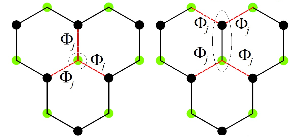
Figure 2: (Color online): Two possible clusters for the solution of the slave rotor. The dotted lines indicate the mean field value of the rotor field connecting the cluster at hand to its neighbours.

Now the remaining challenge is to solve the rotor problem posed by the Hamiltonian (10). One simple way to think of the rotor Hamiltonian is to fix a value for $\ell$ that gives a local Hilbert space dimension of $2\ell+1$ for each rotor. This Hilbert space grows as $N^{2\ell+1}$ where $N$ is the number of lattice sites. However if we further decouple the nearest neighbour terms as

$$e^{-i\theta_{i}+i\theta_{j}}\approx e^{-i\theta_{i}}\langle e^{i\theta_{j}}\rangle+{\rm h.c.}=e^{-i\theta_{i}}\Phi_{j}+{\rm h.c.},$$ (12)

where a mean field rotor variable $\Phi_{j}=\langle e^{i\theta_{j}}\rangle$ is introduced, the rotor problem is considerably simplified. This mean field decomposition can be implemented on various clusters. We consider two types of clusters with finite number of sites denoted in Fig. 2. For the single-site cluster the mean field variables connect a given site to its neighbours on the lattice, and the single-site Hamiltonian has no structure. In this case the mean field rotor Hamiltonian for every site is given by,

$$H_{\theta}^{\rm 1-site~{}MF}=-3\chi_{f}\Phi\left(e^{-i\theta}+e^{i\theta}\right)+\frac{U}{2}\left(n^{\theta}\right)^{2}$$ (13)

where the coefficient of $3$ is due to three neighbours of every single-site (Fig. 2, left side). The explicit matrix representation of the above single-site mean field Hamiltonian is,

$$\left[\begin{array}[]{ccccc}u\ell^{2}&-3\chi_{f}\Phi&0&\ldots&0\\ -3\chi_{f}\Phi^{*}&u(\ell-1)^{2}&-3\chi_{f}\Phi&\ldots&0\\ 0&-3\chi_{f}\Phi^{*}&\ddots&\ldots&\vdots\\ \vdots&\vdots&-3\chi_{f}\Phi^{*}&u(-\ell+1)^{2}&-3\chi_{f}\Phi\\ 0&0&\ldots&-3\chi_{f}\Phi^{*}&u(-\ell)^{2}\end{array}\right]$$ (14)

where for notational brevity we have introduced $u=U/2$. Within the mean field a two-site cluster can also be adopted (see Fig. 2) for which the Hamiltonian becomes,

$${H}_{\theta}^{\rm 2-site~{}MF}=-\chi_{f}\left({{e}^{-i{{\theta}_{1}}}}{{e}^{i{{\theta}_{2}}}}+{{e}^{-i{{\theta}_{2}}}}{{e}^{i{{\theta}_{1}}}}\right)$$

$$-4{{\chi}_{f}}\Phi\left(\cos{{\theta}_{1}}+\cos{{\theta}_{2}}\right)+u{{\left(n_{1}^{\theta}\right)}^{2}}+u{{\left(n_{2}^{\theta}\right)}^{2}}.$$ (15)

The above Hamiltonian operates in the two-particle space represented by $|n^{\theta}_{1},n^{\theta}_{2}\rangle$ where $n^{\theta}_{i}=-\ell_{i}\ldots\ell_{i}$ for $i=1,2$. The effect of the two-site MF Hamiltonian on every such state is given by,

$$-\chi_{f}\left(|n^{\theta}_{1}-1,n^{\theta}_{2}+1\rangle+|n^{\theta}_{1}-1,n^{\theta}_{2}+1\rangle\right)$$

$$-2\chi_{f}\Phi\sum_{a=\pm 1}\left(|n^{\theta}_{1}+a,n^{\theta}_{2}\rangle+|n^{\theta}_{1},n^{\theta}_{2}+a\rangle\right)$$

$$+u\left({n^{\theta}_{1}}^{2}+{n^{\theta}_{2}}^{2}\right)|n^{\theta}_{1},n^{\theta}_{2}\rangle.$$ (16)

The following algorithm self-consistently determines all the mean field parameters: For given set of external parameters such as $U$, (I) Start with an initial guess for $\chi_{f}$. (II-a) For the above $\chi_{f}$, guess a $\Phi$. (II-b) Diagonalize the matrix (14) and obtain its ground state. (II-c) In the obtained ground state update the $\Phi=\langle e^{i\theta}\rangle$ and keep repeating until $\Phi$ is self-consistently determined. (III) For the present value of $\chi_{f}$ and $\Phi$, use Eq. (7) to obtain $\chi_{\theta}$. (IV) Plug in the $\chi_{\theta}$ into the spinon Hamiltonian (9) and diagonalize it. (V) For the ground state of the above spinon Hamiltonian use Eq. (8) to update the initial guess $\chi_{f}$. This procedure is repeated until mean field parameters $\chi_{f},\chi_{\theta},\Phi$ are self-consistently determined. It must be noted that the above procedure is done for a fixed value of $\ell$. One has to repeat the procedure for larger values of $\ell$ to ensure that the final converged results do not change much upon further increase in the dimension of the rotor space. We confirm that as previously noted Paramekanti the choice $\ell=2$ is accurate enough.

Upon increasing the Hubbard interaction $U$ beyond a critical point $U_{b}$ the mean field parameter $\Phi$ vanishes that corresponds to strong fluctuations in the phase variable, and hence frozen fluctuations of the corresponding number operators, i.e. putative Mott state. However, as will be discussed in the next section the phase fluctuations have still have the chance to survive in the form of sign fluctuations that can be captured by enslaving an Ising variable.

III slave spin method

The charge degree of freedom at every site can be described by variety of methods. Description in terms of a rotor variable whose conjugate variable controls the charge state is one possibility. Another appealing possibility is to use an Ising variable to denote the charge state. Using an Ising variable to specify the electric charge can be implemented in various ways Sigrist ; HasanSlaveSpin ; Si . In this section we briefly review the presentation of Ref. Sigrist and adopt it in our investigation of the ionic Hubbard model on the honeycomb lattice.

In this representation an Ising variable $\tau$ is introduced to take care of the charge configuration of every site. Empty and doubly occupied configuration are represented by $|+\rangle$, while singly occupied configurations possessing local moment both are represented by $|-\rangle$ where,

$$\tau^{z}|\pm\rangle=\left(\pm 1\right)|\pm\rangle$$ (17)

The correspondence between physical states and those in the Hilbert space extended by introduction of Ising variables is:

$$\left|{\rm empty}\right\rangle=\left|+\right\rangle\left|0\right\rangle$$

$$\left|{\rm singly~{}occupied},\uparrow\right\rangle=\left|-\right\rangle\left|\uparrow\right\rangle$$

$$\left|{\rm singly~{}occupied},\downarrow\right\rangle=\left|-\right\rangle\left|\downarrow\right\rangle$$

$$\left|{\rm doubly~{}occupied}\right\rangle=\left|+\right\rangle\left|\uparrow\downarrow\right\rangle.$$ (18)

where states on the left hand correspond to physical electrons, and those in the right hand are product of states corresponding to Ising variables, $|\pm\rangle$, and those corresponding to spinon. Creation of each electron has almost a parallel on the right side implying that $c^{\dagger}\sim f^{\dagger}$. However each time an electron is created, the charge state flips between the one having a local moment and the one having no local moment. This corresponds to a flip in the Ising variable that can be achieved with the action of Pauli matrix $\tau^{x}$. Therefore the physical electron at every site $j$ can be represented as,

$$c_{j\sigma}^{\dagger}\equiv\tau^{x}_{j}f_{j\sigma}^{\dagger}.$$ (19)

where $f^{\dagger}_{j\sigma}$ creates a spinon of spin $\sigma$ at site $j$. The fact that creation of each physical charge is synonymous to creation of a spinon implies that the physical charge is basically carried by spinons. This was a key observation made by Nandkishore and coworkers Nandkishore that is formally reflected in Eq. (19) as the fact that the Pauli matrix $\tau^{x}$ being a real matrix can not absorb the $U(1)$ phase transformation that generates the conservation of charge, and hence all the charge of electron is carried by the spinon.

The Hilbert space represented by the product of Ising pseudo-spin and spinon spaces is larger than the physical space and includes states such as $|+\rangle|\uparrow\rangle$, etc that do not correspond to any physical state. Inspection shows that those states can be eliminated by the following constraint:

$$\tau^{z}_{j}+1-2(n_{j}-1)^{2}=0.$$ (20)

In this new representation the ionic Hubbard Hamiltonian becomes,

$$H=-\sum\limits_{\langle ij\rangle}\tau_{i}^{x}\tau_{j}^{x}f_{i\sigma}^{\dagger}f_{j\sigma}+\frac{U}{4}\sum_{j}{\left(\tau_{j}^{z}+1\right)}$$

$$+\Delta\sum_{j}f^{\dagger}_{j\sigma}f_{j\sigma}(-1)^{j}$$ (21)

where as before the hopping $t$ of the physical electrons is set as the unit of energy and the constraint Eq. (20) has enabled us to cast the Hubbard $U$ into a form involving only Ising variable $\tau^{z}$. Again in the ionic potential term the Ising pseudo-spins being squared to unit matrix cancel each other and hence the staggered ionic potential is only coupled to the spinons. Mean-field decoupling of the Ising and spinon variables is lead to two separate Hamiltonians governing the dynamics of spinons $f$ and Ising variables $\tau$ as follows:

$$H_{f}= -\sum\limits_{ij}{{{\chi}_{I}}f_{i\sigma}^{\dagger}{{f}_{j\sigma}}}+\Delta\sum_{j}f^{\dagger}_{j\sigma}f_{j\sigma}(-1)^{j}$$

$$-2\lambda^{\prime}\sum_{j}\left(f^{\dagger}_{j\uparrow}f_{j\uparrow}+f^{\dagger}_{j\downarrow}f_{j\downarrow}-1\right)^{2},$$ (22)

and

$$H_{\rm ITF}=-\chi^{\prime}_{f}\sum\limits_{ij}\tau_{i}^{x}\tau_{j}^{x}+\left(\frac{U}{4}+\lambda^{\prime}\right)\sum\limits_{i}{\tau_{i}^{z}},$$ (23)

where the two Hamiltonians are coupled to each other through the following self-consistency equations:

$$\chi_{I}=\langle\tau^{x}_{i}\tau^{x}_{j}\rangle,$$ (24)

$$\chi^{\prime}_{f}=\langle f^{\dagger}_{i\sigma}f_{j\sigma}\rangle,$$ (25)

and the Lagrange multiplier $\lambda^{\prime}$ is introduced to implement the constraint (20) on average. As can be seen, within the present representation, the fermion part, (22) still remains an interacting problem of the Hubbard type, where the scale of on-site interaction among the spinons is set by the Lagrange multiplier $\lambda^{\prime}$. The mean field approximation lends itself on the assumption that the system in the enlarged Hilbert space is a product state composed of a spinon part and an Ising part. The spinon part of the wave function is expected have a form close to an Slater determinant and hence the parameter $\lambda^{\prime}$ is expected to represent a small residual interactions between the spinons. Approximate strategies to handle the interacting spinons have been suggested and discussed in Ref. Sigrist . With this argument we reckon that it is reasonable to assume $\lambda^{\prime}=0$ as an approximate strategy to obtain the simplest possible solution Fiet .

To understand the nature of the approximation $\lambda^{\prime}\approx 0$, let us focus on some special lucky situations where it can be proven that $\lambda^{\prime}=0$ is exact. When the ionic term is absent, i.e. for the pure Hubbard model one may have situations where the partition function $Z$ happens to be an even function of $U$, such as the particle-hole symmetric case considered here michele2011 ; michele2015 . In this case, first of all the Hubbard interaction at half-filling can be written as,

$$Un_{j\uparrow}n_{j\downarrow}-\frac{U}{2}\left(n_{j\uparrow}+n_{j\downarrow}\right),$$ (26)

where due to half-filling condition the chemical potential $\mu=U/2$ is used and the site index has been dropped for simplicity. Under a particle-hole transformation in one spin sector only (let us call it PH$\sigma$ transformation in this paper), namely,

$$c^{\dagger}_{j\uparrow}=\tilde{c}^{\dagger}_{j\uparrow},~{}~{}~{}c^{\dagger}_{j\downarrow}=(-1)^{j}\tilde{c}_{j\downarrow},$$ (27)

where $(-1)^{j}=\pm 1$ depends on whether it is on sublattice A, or B. Under PH$\sigma$ the role of charge and spin density are exchanged, namely $n_{\uparrow}+n_{\downarrow}\to\tilde{n}_{\uparrow}-\tilde{n}_{\downarrow}$. This transformation maps the particle-hole symmetric Hubbard interaction of Eq. (26) to,

$$\tilde{U}\tilde{n}_{j\uparrow}\tilde{n}_{j\downarrow}-\frac{\tilde{U}}{2}\left(\tilde{n}_{j\uparrow}+\tilde{n}_{j\downarrow}\right)$$ (28)

which is nothing but the original Hubbard interaction at half-filling with the only difference that $\tilde{U}=-U$. At half-filling under the PH$\sigma$ transformation is a symmetry of the Hubbard model which implies properties of system are even with respect to Hubbard $U$.

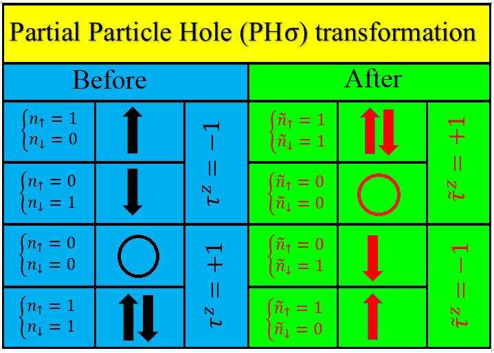
Figure 3: (Color online): Schematic summary of partial particle-hole transformation, PH$\sigma$ that affects only down-electrons. It basically exchanges the local charge and spin densities. In a setting with one Anderson impurity, the PH$\sigma$ would correspond to transformation between spin and charge Kondo effects.

Let us now examine how does the constraint (20) behave under the PH$\sigma$ transformation. As indicated in the Fig. 3 the role of PH$\sigma$ transformation in terms of Ising pseudo-spins is to exchange the role of $|+\rangle$ and $|-\rangle$ states of Ising variables. Therefore the effect of PH$\sigma$ transformation on any operator ${\cal O}$ that contains Ising variables is to change ${\cal O}\to\tau^{x}{\cal O}\tau^{x}$. This transformation leaves the first term in the ITF Hamiltonian (23) intact, but it changes the second term at a given site as follows:

$$\left(\frac{U}{4}+\lambda^{\prime}\right)\tau^{z}\to\left(\frac{U}{4}+\lambda^{\prime}\right)\tau^{x}\tau^{z}\tau^{x}$$

$$=-\left(\frac{U}{4}+\lambda^{\prime}\right)\tau^{z}=-\left(-\frac{U}{4}+\lambda^{\prime}\right)\tau^{z},$$ (29)

where in the last equality we have used the fact that the Hubbard model at half-filling is even with respect to Hubbard $U$. Therefore we have proven that at half-filling for the Hubbard model, the Lagrange multiplier $\lambda^{\prime}$ is exactly zero.

Turning on the ionic potential $(-)^{j}\Delta(n_{\uparrow}+n_{\downarrow})$, the PH$\sigma$ transformation maps to $(-)^{j}\Delta(\tilde{n}_{j\uparrow}-\tilde{n}_{j\downarrow})$, i.e. the charge density is mapped to spin-density. Therefore the PH$\sigma$ is not a symmetry of ionic Hubbard model at half-filling. Hence the partition function has both even and odd parts as a function of $U$. This prevents the Lagrange multiplier $\lambda^{\prime}$ from becoming zero. However the above symmetry consideration suggests that the physics of ionic (and repulsive) Hubbard model maps onto the physics of attractive Hubbard model in the presence of a staggered magnetization field (since it is coupled to spin density in staggered way). Another merit of the above symmetry discussion is that based on the following argument in Ref. michele2011 , we can infer what is precisely missed by the approximation $\lambda^{\prime}=0$: Let us rewrite the constraint (20) as,

$${\cal P}_{+}=1+\tau^{z}_{j}\Omega_{j}=0,~{}~{}~{}\Omega_{i}=1-2(n_{j}-1)^{2},$$ (30)

which identifies the operator $\Omega_{j}$ as the fluctuations of the charge away from half-filling. It was shown in Ref. michele2011 that to all orders in perturbation theory, the term $1$ in ${\cal P}_{+}$ contributes only in even powers of $U$ while the second term contributes only in odd powers of $U$. Therefore for a half-filled situation of the pure Hubbard model, the effect of second term is nullified, and basically one need not worry about projection. This is another way of saying that the Lagrange multiplier $\lambda^{\prime}$ at half-filling becomes zero. By adding ionic term to the half-filled Hubbard model, or placing the Hubbard model itself away from half-filling, $\lambda^{\prime}$ is expected to be small based on our earlier argument on small residual interactions. In this case using the approximation $\lambda^{\prime}\approx 0$ amounts to missing the effects that are odd functions of the Hubbard $U$.

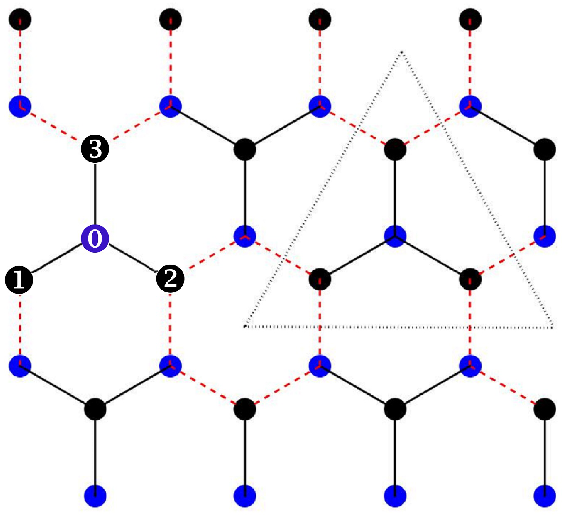
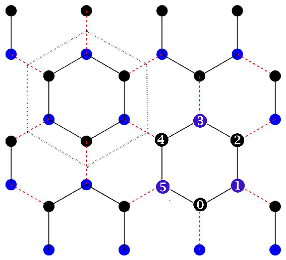
Figure 4: (Color online) Two choices for the cluster mean field treatment of the slave Ising pseudo-spins; the Y shaped (left) and hexagonal cluster (right).

Within the approximation of $\lambda^{\prime}=0$, the spinon part describes a non-interacting band of spinons whose bandwidth is renormalized by the $\chi_{I}$ parameter obtained from the Ising part. The physics of transition to orthogonal state is then captured by the disordering transition of the Ising sector (23) where vanishing quasi-particle weight of the physical electrons are characterized by $\langle\tau^{x}\rangle=0$ Nandkishore ; michele2015 .

In the absence of the ionic term, i.e. when $\Delta=0$, both ordered and disordered side of the ITF Hamiltonian (23) are conducting state: (i) If the underlying rotors are ordered, namely $\langle e^{i\theta}\rangle\neq 0$ the conducting state within the Hubbard model is a Fermi liquid. This holds for $U<U_{b}$. (ii) When the rotor order vanishes beyond $U_{b}$, i.e. $\langle e^{i\theta}\rangle=0$ still we may have $\langle\tau^{x}\rangle\neq 0$ which again is a conducting state (Ising metal) for the pure Hubbard model. This state persists until $U_{\perp}$ where the Ising order vanishes and the pure Hubbard model describes the orthogonal metallic state. By adding the ionic term $\Delta$, it is crucial to note that on-site ionic potential does not couple to neither slave Ising variables, nor to the salve rotor variables. However, the effect of the ionic potential $\Delta$ is to modify the order parameters through the mean field self-consistency equations, but their order-disorder physics remains the same as the Hubbard model as the ionic term does not explicitly appear in the Ising or rotor sectors. The essential role of the ionic term is to create Bragg reflections in the spinon Hamiltonian and to gap them out which corresponds to rendering Fermi liquid, Ising metal and orthogonal metal phase of the pure Hubbard model to band insulator, Ising band insulator, and orthogonal insulator, respectively.

The disordering phase transition of the Ising Hamiltonian (23) can be captured within a simple cluster mean field approximation. Let us decompose the lattice to clusters $\Gamma$ labeled by integer $I$ whose internal sites are labeled by integers $a,b$ etc. Then the Ising variables are denoted by $\vec{\tau}_{\Gamma,a}$. With this re-arrangements, and after mean field decoupling of the cluster with its surrounding sites via a mean field order parameter $m=\langle\tau^{x}\rangle$ (see Fig. 4), the Ising part becomes,

$$H=\sum_{\Gamma}H_{\Gamma},$$ (31)

where the Hamiltonian for cluster $\Gamma$ is,

$$H_{\Gamma}=-\chi^{\prime}_{f}\sum_{a,b\in\Gamma}\tau_{\Gamma,a}^{x}\tau_{\Gamma,b}^{x}-\frac{mz}{2}\sum_{a\in\Gamma}\tau_{\Gamma,a}^{x}+\frac{U}{4}\sum_{a}{\tau_{\Gamma,a}^{z}}.$$ (32)

In this cluster Hamiltonian, the $z$ denotes number of bonds crossing the boundary of the cluster. The factor $1/2$ avoids double counting and $m=\langle\tau^{x}\rangle$ is the Ising order parameter that at the mean field level decouples the cluster $\Gamma$ from its surroundings, but the interactions within the cluster $\Gamma$ are treated with exact diagonalization. In Fig. 4 we have depicted clusters used in the present work. For more details on the construction of the Hilbert space and diagonalization of the Hamiltonian, please refer to the Appendix. The Ising disordering considered here for 4-site and 6-site clusters do now show appreciable difference. In this work we report the critical values $U_{c}$ of the Ising disordering transition that is obtained from 6-site clusters.

IV Results

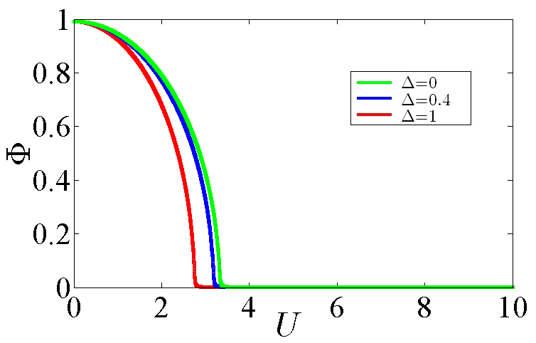
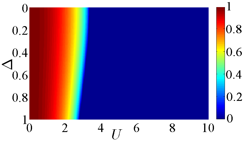
Figure 5: (Color online) The slave rotor order parameter $\Phi$. The right panel shows the intensity plot in the plane of Hubbard $U$ and ionic potential $\Delta$ on the honeycomb lattice. The left panel shows the dependence of $\Phi(U)$ for some selected values of $\Delta$ as indicated in the legend. The rotor (single boson) condensate is lost at $U_{b}$.

In Fig. 5 we have plotted the results of a slave-rotor mean field for a two-site cluster. The rotor Hilbert space in this plot has been constructed for the angular momentum $\ell=2$. We have checked that the results are not sensitive to increase in the size of the rotor Hilbert space beyond $\ell=2$. The left panel shows the evolution of order parameter $\Phi$ of rotors as a function of Hubbard $U$ for a selected set of ionic potentials indicated in the legend. As can be seen for $\Delta=0$ the critical value $U_{b}$ starts around $3.5$ and decreases by increasing $\Delta$. At $\Delta=1$ the critical value for the disordering of single-boson is around $2.8$ . This means that in the presence of a staggered potential it becomes easier to loos the single-boson condensate whereby the Ising phase (paired boson superfluid) starts. Right panel in the figure provides an intensity map of the rotor order parameter in the $(U,\Delta)$ plane. The blue region corresponds to zero single-boson condensation amplitude, and the red corresponds to maximal (i.e. 1) condensation amplitude for the single-bosons $\langle e^{i\theta}\rangle$.

In Fig. 6 we present the cluster mean field results for the Ising order parameter. The left panel shows the Ising magnetization $m=\langle\tau^{x}\rangle$ as a function of $U$ for selected values of the staggered potential $\Delta$ indicated in the figure. The right panel provides an intensity map of the Ising order parameter in the $(U,\Delta)$ plane. The color code is the same as in Fig. 5. Once the Ising order goes away, we are in the orthogonal phase. By increasing the staggered ionic potential from $\Delta=0$ to $\Delta=1$, the critical value $U_{c}$ decreases from $\sim 6.9$ to $5.7$. This trend is similar to the behavior of rotor order parameter, i.e. the effort of $U$ to destroy the Ising order parameter $m=\langle\tau^{x}\rangle$ is assisted by the ionic potential $\Delta$. This points to the fact that getting both IBI and OBI is facilitated by ionic potential $\Delta$. Larger the ionic potential, easier to ”quantum melt” the 1- and 2- boson condensates that correspond to entering Ising and orthogonal phases.

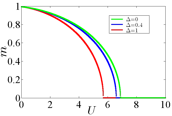
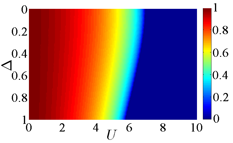
Figure 6: (Color online) The slave spin order parameter $m=\langle\tau^{x}\rangle$. The right panel shows the intensity plot of the Ising order parameter $m$ as a function of $U$ and $\Delta$. Right panel shows the variations in the Ising order parameter as a function of $U$ for some selected values of $\Delta$ indicated in the legend. The data are obtained within the cluster mean field approximation for a 6-site cluster.

Fig. 7 combines Figs. 5 and 6 and shows that there is a clear region $U_{b}\leq U<U_{\perp}$ where the rotor order parameter is zero, i.e. the single boson condensate has vanished, while the Ising order parameter is non-zero, i.e. the double boson is condensed Nandkishore . In the region $U<U_{b}$ the underlying metallic state is a normal fermi liquid which is gapped out by directly coupling to the staggered potential and therefore the underlying Fermi liquid state becomes a normal band insulator. For $U_{b}<U<U_{\perp}$ the 1-boson condensate vanishes, and interaction between the bosons leads to pairing of bosons and the 2-boson condensates forms. In this region due to formation of two-boson pairs that admit a $Z_{2}$ gauge structure, the charge fluctuations are controlled by Ising variable which is ordered and gives IBI. The Ising order parameter vanishes at $U_{\perp}$ beyond which the semiconducting transport will be entirely done by spinons. For largest values of $U>U_{\rm Mott}$ the system eventually becomes Mott insulating Ebrahimkhas .

The existence of a region where the Ising variable is ordered, but the rotor variable is disordered endows the non-Mott phase of the ionic Hubbard model with a condensate of paired charge bosons whence charge fluctuations survive in the form of Ising variables. In the ionic Hubbrard model this corresponds to Ising band insulating phase where the kinetic energy of spinon Hamiltonian is controlled by an Ising order parameter, and hence the band properties of such a semiconducting phase inherits characteristic temperature and field dependence from the underlying Ising model. Across the Ising transition, the quasi-particle weight of the physical electron is lost, and the electric charge is carried by spinons which corresponds to loosing the Ising condensate. This is the orthogonal phase which in the ionic Hubbard model corresponds to OBI. The quasiparticle weight of the physical electrons in this phase vanishes as it is controlled by the Ising order parameter Nandkishore , and hence in the OBI phase the states at the bottom of the conduction and top of the valence band are not visible by ARPES. However, since the current operators is solely constructed by the spinons, the optical conductivity (i.e. the current-current correlation function) does couple to the states near the bottom of conduction band and those near the top of the valence band of the resulting OBI. Therefore an important characteristic property of OBI is that the optical conductivity gap is expected to be smaller than the ARPES gap. For the two-dimensional semiconductors or insulators the ability to tune the chemical potential into the conduction band provides a chance to examine such an ”ARPES-dark stats” by quantum oscillations experiments. Once the chemical potential is tuned to the conduction band, the thermally excited carriers into the ARPES-invisible states at the bottom of the conduction band would display quantum oscillations. The ”ARPES-dark” states of the OBI phase would couple to thermal probes as well which means that the gap extracted from thermal measurements will be smaller than the ARPES gap.

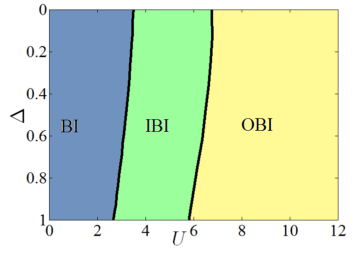
Figure 7: (Color online): Phase diagram of the ionic Hubbard model within the present combination of slave-rotor and slave-spin mean field approximations.

V Discussions and summary

We have investigated the phase transitions of the ionic Hubbard model on the honeycomb lattice using a combination of slave rotor and slave spin mean field theories. The phase diagram of the ionic Hubbard model on the honeycomb lattice within the present method is shown in Fig. 7. For small values of Hubbard $U<U_{b}$ (blue phase) we find a normal band insulating (semiconducting) state. For intermediate values of $U_{b}<U<U_{\perp}$ (green phase) the properties of the band insulating phase is controlled by an Ising condesate amplitude. In this band insulator the rotor is disordered, $\langle e^{i\theta}\rangle=0$, but the Ising variables remains ordered, $\langle\tau^{x}\rangle\neq 0$. The interesting nature of this phase lends itself on the chargon pairing Nandkishore . By further increasing $U$ the Ising order is lost, and we end up in even more exotic orthogonal phase (yellow phase) where the chargon pair condensate has vanished and hence semiconducting transport is dominated by spinons. The spinons inherit the electric charge of the electron. This is simply because the $U(1)$ symmetry (charge conservation) of the original ionic Hubbard model can not be incorporated into the Ising pseudo-spins (as they are real matrices), the $f$ operator inherits the electric charge of electrons and a set of conduction-valence bands of spinons is left for semiconductor transport. Therefore yellow phase in Fig. 7 can be viewed as a spinon semiconductor.

Now suppose that we are given a semiconducting (band insulating) sample. How do we differentiate whether it is BI, IBI, or OBI? (i) Let us start with OBI (yellow region in Fig. 7): Since vanishing of the Ising order amounts to loosing the quasi-particle weight of the physical electron, the defining property of the orthogonal (yellow) phase is that the ARPES gap is larger than the optical gap as the former probe couples to electrons whose quasiparticle weight is lost in the orthogonal phase while the later probe couples to the spinon current operator. The same holds for the thermal gap. In the semiconducting phase the gap can be extracted from thermal measurements as well. Again this is expected to be smaller than the ARPES gap which signals existence of ARPES-dark states which are nothing but the spinon states. This criterion not only qualifies a given sample as OBI, but also from fundamental physics point of view can serve as a proof of quantum number fractionization phenomena.

(ii) The essential property of the Ising phase (green region in Fig. 7) is that it depends on an Ising order parameter $m=\langle\tau^{x}\rangle$. Due to the temperature dependence of underlying (slave) Ising order parameter that multiplies the kinetic energy of spinons, the effective mass will correspondingly acquire a temperature dependence characteristic of the Ising order. This can be detected by standard cyclotron resonance experiments and monitoring their temperature dependence $m^{*}(T)$. Particularly when the temperature is high enough to hit the ”thermal” disordering point of the Ising variable $\langle\tau^{x}\rangle$, or when $U$ is close to $U_{\perp}$, the cyclotron effective mass is expected to be enhances as one approaches the OBI phase from the IBI side. The characteristic Ising power-laws of the Ising universality class are expected to leave their footprint in the temperature dependence of the effective mass. This situation is in sharp contrast to normal semiconductors where band parameters are almost rigid and do not depend on the temperature. In normal semiconductors the dominant temperature dependence determining the transport properties appears in the density of excited carriers, while in the Ising semiconductor, in addition to the carrier density, every property involving the Ising order parameter acquires an additional and distinctive temperature dependence. This can serve not only to distinguish orthogonal semiconductors/insulators from their normal relatives, but also as a existence proof for the underlying Ising variable and hence the fractional nature in two-dimensional semiconductors with strong correlations.

(iii) The Ising phase may have anomalous response to applied magnetic fields. Although the Ising variable $\tau^{z}$ labels the charge states, nevertheless it carries information about the local moments. The $\tau^{z}=+1$ state carries no net magnetic moment and hence in the first order, it does not couple to an external magnetic field $B$. However the $\tau^{z}=-1$ charge state carries a net local moment and hence can Zeeman couple to $B$ to gain energy. In this way, the applied $B$ field effectively couples to Ising condensate. This may provide extra sensitivity to $B$ field in Ising semiconductors as opposed to normal semiconductors. Given that the resistivity of rare earth monochalcogenides is very sensitive to applied magnetic fields, and that the heavy Fermion elements involved are qualified for strong correlations, we suspect that rare earth semiconducting systems such as Europium monochalcogenides EuX or Samarium monochalcogenides SmX where X=S, Se, Te Smirnov and rare earth nitrides Sclar can be interesting platforms to search for signatures of underlying Ising condensate.

Let us briefly discuss the connection of the present work to other works on the ionic Hubbard model. Investigations of the nature of intermediate phase in the ionic Hubbard model fall into two major groups: First group suggests that the intermediate phase is gapped, while the second group suggests gapless intermediate state. The present work also does find a gapped intermediate phase. However, the gap in the present case is due to symmetry breaking in a fractional degree of freedom. This order does not correspond to any spin or charge density as no form of density operator depends on the Ising pseudo-spin simply because $\tau^{x}$ squares to unit matrix. The gap in the Ising and orthogonal semiconductor is caused by the Bragg reflection of spinons, and as such there are no low-energy Goldstone modes associated with our present proposal. The second group of investigations suggest a gapless state for a region $\Delta\sim U$. Within the present mean field approach, we get three gapped phases depicted in Fig. 7: BI (blue), IBI (green) and OBI (yellow. The present approach does not capture the Mott phase as in the mean field and within the half-filled Hubbard model we do not take interactions among spinons of the IBI phase into account. However a comparison between our previous dynamical mean field theory (DMFT) result is rewarding Ebrahimkhas . Within the DMFT approach the battle between $U$ and $\Delta$ to close the gap takes place. The dashed lines in Fig. 8 represent the phase boundaries from DFMT. The left branch of the dashed line separates band insulator from semi metal (SM) while the right branch of the dashed phase boundary separates SM from Mott insulator (MI). The intermediate phase is a massless Dirac phase within the DMFT. When we superimpose the DMFT phase diagram Ebrahimkhas with that of Fig. 7 we find that the phase boundaries obtained from present study (bold lines) partition the BI and SM phase of the DMFT phase diagram into three phase corresponding to normal, Ising and orthogonal variants. Although these are two different methods, and critical values obtained from DMFT and present studies maybe correspond to different mechanisms, but that does not concern us here. Improvements in the approximations may push the bold lines slightly away, but does not change the fact that the bold phase boundaries cross the left branch of the DMFT (dashed boundary). This comparison sheds a new light: Realization of IBI and OBI phases requires large enough ionic potential. For very small ionic potentials, the DMFT battle between $U$ and $\Delta$ can possibly kill the insulating phase, and give a massless SM. Then increase in Hubbard $U$ will give rise to Ising semi metal (ISM) or orthogonal semi metal (OSM) Chinese . If the ionic potential grows further, the green phase in the band insulating side also gets a chance and therefore IBI could be realized if $\Delta$ is larger than about $\sim 0.1$ (in units of hopping $t$ of course). If we keep increasing $\Delta$ beyond $\sim 0.38$ the OBI phase also gets a chance. However if the DMFT scenario of battle between $U$ and $\Delta$ suggests that the OBI phase does not directly transform into Mott phase, but instead goes through an orthogonal semi metal which is appealing: The battle will continue in the fractionalized OBI phase of spinons and can presumably close the spinon gap in OBI to render it OSM before getting into Mott phase Ebrahimkhas .

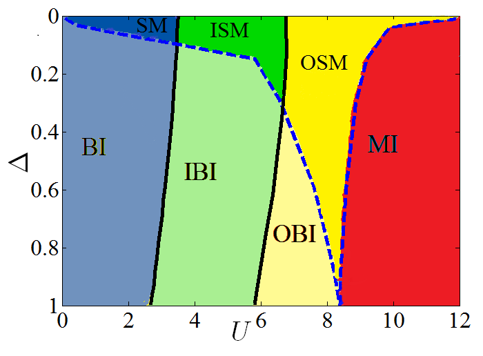
Figure 8: (Color online): Comparison between the present mean field phase diagram and our previous DMFT phase diagram. The dashed lines correspond to DMFT results. Competition between $U$ and $\Delta$ in DMFT scenario gives a massless Dirac phase between the two dashed lines. Rotor and Ising transitions partition the massless Dirac phase into semi-metal (SM), Ising semi metal (ISM) and orthogonal (SM). For discussions see the text.

Within the present mean field approximate treatment of the IBI-OBI phase transition, the thermal probes are coupled to spinons that are independent of Ising pseudo-spins. The optical probe on the other hand always couples to the spinons. However going beyond the mean field by properly taking the fluctuations of internal gauge fields that glue the spinons to Ising field into account is expected to provide corrections to the present picture. Therefore thorough investigation of gauge fluctuations and its effect on the physical properties of Ising and orthogonal phases remains and is worth to be explored. Thinking along the schematic table of Fig. 1 one may also wonder about other possible columns to start with at $U=0$. An interesting possibility can be the Ising and orthogonal cousin of the Anderson insulator, where the insulating behavior at $U=0$ is due to randomness. This will add another interesting aspect to the Mott-Anderson problem, namely the interplay between the Hubbard $U$ and randomness around $U_{c}^{\perp}$, and possible glassy phases of spinons. This problem is currently under investigation in our group Amini .

Let us emphasize that although in the present paper we are confined to zero temperature where the quantum phase transition between IBI and OBI is driven by Hubbard $U$ by destroying the Ising condensate; the quantum fluctuations are not the only way to destroy a condensate. Thermal fluctuations can be conveniently employed to achieve this goal. Within this scenario, once a system is found in IBI phase, simply rising the temperature gives a chance to the OBI phase. If the anomalous magnetic field dependence of the transport properties in monochalcogenides Sclar ; Smirnov is due to the Ising order, then searching for ”ARPES-dark” states in elevated temperature can support this assumption. By increasing the temperature, once the underlying Ising order is lost, the ARPES gaps starts to deviate from thermal gap. Moreover since the effective mass of spinons in the IBI is controlled by Ising order parameter the cyclotron mass will acquire a characteristic Ising-like temperature dependence.

To conclude, additional temperature and magnetic field dependence due to an underlying Ising order parameter that is attached to spinons is the key feature of transition to orthogonal phase. This observation suggests that the correlated semiconductors maybe an alternative and appealing (if not superior) rout to search for correlation driven phenomena where the sensitivity of semiconducting carrier density to temperature combined with the temperature dependence of underlying Ising order field cooperate to reveal information about fractional excitation of solids. Indeed in the absence of tunability of the correlation parameter $U$ in solids, further dependence of the underlying Ising field to temperature and magnetic field can serve as conveniently tunable parameters to probe fractional excitations in correlated semiconductors. Investigation of inhomogeneity and impurities in spinon-semiconductors and their contrast to normal semiconductors can shed light on exotic properties of spinon semiconductors. From technological point of view, given the very extensive use of semiconductors in every day life, further exploration of the exotic properties of spinon semiconductors may prove useful.

VI Acknowledgements

We thank A G Moghaddam for useful comments and R. Ghadimi for very helpful discussions. TF appreciates the Ministry of Science, Research and Technology (MSRT) of Iran for financial support during a visit to Sharif University of Technology.

Appendix A Details of exact diagonalization for clusters

In this appendix we present details of the exact diagonalization for the ITF Hamiltonian on a finite cluster for 4 and 6 site clusters. We employ group theory methods to reduce the dimension of ensuing matrices.

A.1 Y-shaped 4-site cluster

To solve the Eq. (32) first we choose a Y-shaped 4-site cluster $\Gamma$ shown in Fig. 9. The spin variables at every site have two possible states giving a total of $2^{4}-16$ possible states for the cluster $\Gamma$. Each state of this cluster is of the form $|\sigma_{3},\sigma_{2},\sigma_{1},\sigma_{0}\rangle$ where $\sigma_{a}$ can take two possible values $\uparrow,\downarrow$ and the site indices $a=0,1,2,3$ are indicated in Fig. 9. The basis in this 16-dimensional Hilbert space are as follows (for brevity we have dropped $|\rangle$ from the representation of basis states):

$$\left|1\right\rangle=\uparrow\uparrow\uparrow\uparrow~{}~{}\left|2\right\rangle=\uparrow\uparrow\uparrow\downarrow~{}~{}\left|3\right\rangle=\uparrow\uparrow\downarrow\uparrow~{}~{}\left|4\right\rangle=\uparrow\downarrow\uparrow\uparrow$$ (33)

$$\left|5\right\rangle=\downarrow\uparrow\uparrow\uparrow~{}~{}\left|6\right\rangle=\uparrow\uparrow\downarrow\downarrow~{}~{}\left|7\right\rangle=\uparrow\downarrow\downarrow\uparrow~{}~{}\left|8\right\rangle=\downarrow\downarrow\uparrow\uparrow$$

$$\left|9\right\rangle=\downarrow\uparrow\uparrow\downarrow~{}~{}\left|10\right\rangle=\uparrow\downarrow\uparrow\downarrow~{}~{}\left|11\right\rangle=\downarrow\uparrow\downarrow\uparrow~{}~{}\left|12\right\rangle=\uparrow\downarrow\downarrow\downarrow~{}~{}$$

$$\left|13\right\rangle=\downarrow\uparrow\downarrow\downarrow~{}~{}\left|14\right\rangle=\downarrow\downarrow\uparrow\downarrow~{}~{}\left|15\right\rangle=\downarrow\downarrow\downarrow\uparrow~{}~{}\left|16\right\rangle=\downarrow\downarrow\downarrow\downarrow$$

In the 4-site cluster of Fig. 9 the positions $1,2,3$ are not nearest neighbours of each other, while they are all neighbours of the site $0$. So the exchange interaction in the cluster takes place only between the site $0$ and the above three sites. Hence the first term of Eq. (32) for the 4-site cluster is,

$${{H}_{1}}=-\sum\limits_{\langle a,b\rangle\in\Gamma}{\tau_{a}^{x}\tau_{b}^{x}=-\left\{\tau_{0}^{x}\tau_{1}^{x}+\tau_{0}^{x}\tau_{2}^{x}+\tau_{0}^{x}\tau_{3}^{x}\right\}}.$$ (34)

The effect of the above term on the bases is:

$${{H}_{1}}\left|1\right\rangle=-\left\{\left|6\right\rangle+\left|9\right\rangle+\left|10\right\rangle\right\}$$

$${{H}_{1}}\left|2\right\rangle=-\left\{\left|3\right\rangle+\left|4\right\rangle+\left|5\right\rangle\right\}$$

$${{H}_{1}}\left|3\right\rangle=-\left\{\left|2\right\rangle+\left|12\right\rangle+\left|13\right\rangle\right\}$$

$${{H}_{1}}\left|4\right\rangle=-\left\{\left|2\right\rangle+\left|12\right\rangle+\left|14\right\rangle\right\}$$

$${{H}_{1}}\left|5\right\rangle=-\left\{\left|2\right\rangle+\left|13\right\rangle+\left|14\right\rangle\right\}$$

$${{H}_{1}}\left|6\right\rangle=-\left\{\left|1\right\rangle+\left|7\right\rangle+\left|11\right\rangle\right\}$$

$${{H}_{1}}\left|7\right\rangle=-\left\{\left|6\right\rangle+\left|10\right\rangle+\left|16\right\rangle\right\}$$

$${{H}_{1}}\left|8\right\rangle=-\left\{\left|9\right\rangle+\left|10\right\rangle+\left|16\right\rangle\right\}$$

$${{H}_{1}}\left|9\right\rangle=-\left\{\left|1\right\rangle+\left|8\right\rangle+\left|11\right\rangle\right\}$$

$${{H}_{1}}\left|10\right\rangle=-\left\{\left|1\right\rangle+\left|7\right\rangle+\left|8\right\rangle\right\}$$

$${{H}_{1}}\left|11\right\rangle=-\left\{\left|6\right\rangle+\left|9\right\rangle+\left|16\right\rangle\right\}$$

$${{H}_{1}}\left|12\right\rangle=-\left\{\left|3\right\rangle+\left|4\right\rangle+\left|15\right\rangle\right\}$$

$${{H}_{1}}\left|13\right\rangle=-\left\{\left|3\right\rangle+\left|5\right\rangle+\left|15\right\rangle\right\}$$

$${{H}_{1}}\left|14\right\rangle=-\left\{\left|4\right\rangle+\left|5\right\rangle+\left|15\right\rangle\right\}$$

$${{H}_{1}}\left|15\right\rangle=-\left\{\left|12\right\rangle+\left|13\right\rangle+\left|14\right\rangle\right\}$$

$${{H}_{1}}\left|16\right\rangle=-\left\{\left|8\right\rangle+\left|11\right\rangle+\left|12\right\rangle\right\}.$$ (35)

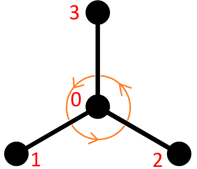
Figure 9: The Y-shaped 4-site cluster chosen in the exact diagonalization of ITF Hamiltonian. The total Hilbert space of this cluster is $2^{4}=16$ dimensional labeled by four spins $|\sigma_{0},\sigma_{1},\sigma_{2},\sigma_{3}\rangle$ where $\sigma_{i}=\uparrow,\downarrow$.

The second term of the cluster Hamiltonian (32) is

$${{H}_{2}}=-\frac{mz}{2}\sum_{a\in\Gamma}{\tau_{a}^{x}}=-\frac{mz}{2}\left\{\tau_{0}^{x}+\tau_{1}^{x}+\tau_{2}^{x}+\tau_{3}^{x}\right\}$$ (36)

where $m$ is the Ising magnetization coupling the boundary sites of the cluster to boundary sites of neighbouring clusters and $z$ is the number of bonds connecting boundary sites $1,2,3$ to other clusters which for this cluster is $z=2$. The effect of $H_{2}$ on the bases is given by,

$${{H}_{2}}\left|1\right\rangle=-m\left\{\left|2\right\rangle+\left|3\right\rangle+\left|4\right\rangle+\left|5\right\rangle\right\}$$

$${{H}_{2}}\left|2\right\rangle=-m\left\{\left|1\right\rangle+\left|6\right\rangle+\left|9\right\rangle+\left|10\right\rangle\right\}$$

$${{H}_{2}}\left|3\right\rangle=-m\left\{\left|1\right\rangle+\left|6\right\rangle+\left|7\right\rangle+\left|11\right\rangle\right\}$$

$${{H}_{2}}\left|4\right\rangle=-m\left\{\left|1\right\rangle+\left|7\right\rangle+\left|8\right\rangle+\left|10\right\rangle\right\}$$

$${{H}_{2}}\left|5\right\rangle=-m\left\{\left|1\right\rangle+\left|8\right\rangle+\left|9\right\rangle+\left|11\right\rangle\right\}$$

$${{H}_{2}}\left|6\right\rangle=-m\left\{\left|2\right\rangle+\left|3\right\rangle+\left|12\right\rangle+\left|13\right\rangle\right\}$$

$${{H}_{2}}\left|7\right\rangle=-m\left\{\left|3\right\rangle+\left|4\right\rangle+\left|12\right\rangle+\left|15\right\rangle\right\}$$

$${{H}_{2}}\left|8\right\rangle=-m\left\{\left|4\right\rangle+\left|5\right\rangle+\left|14\right\rangle+\left|15\right\rangle\right\}$$

$${{H}_{2}}\left|9\right\rangle=-m\left\{\left|2\right\rangle+\left|5\right\rangle+\left|13\right\rangle+\left|14\right\rangle\right\}$$

$${{H}_{2}}\left|10\right\rangle=-m\left\{\left|2\right\rangle+\left|4\right\rangle+\left|12\right\rangle+\left|14\right\rangle\right\}$$

$${{H}_{2}}\left|11\right\rangle=-m\left\{\left|3\right\rangle+\left|5\right\rangle+\left|13\right\rangle+\left|15\right\rangle\right\}$$

$${{H}_{2}}\left|12\right\rangle=-m\left\{\left|6\right\rangle+\left|7\right\rangle+\left|10\right\rangle+\left|16\right\rangle\right\}$$

$${{H}_{2}}\left|13\right\rangle=-m\left\{\left|6\right\rangle+\left|9\right\rangle+\left|11\right\rangle+\left|16\right\rangle\right\}$$

$${{H}_{2}}\left|14\right\rangle=-m\left\{\left|8\right\rangle+\left|9\right\rangle+\left|10\right\rangle+\left|16\right\rangle\right\}$$

$${{H}_{2}}\left|15\right\rangle=-m\left\{\left|7\right\rangle+\left|8\right\rangle+\left|11\right\rangle+\left|16\right\rangle\right\}$$

$${{H}_{2}}\left|16\right\rangle=-m\left\{\left|12\right\rangle+\left|13\right\rangle+\left|14\right\rangle+\left|15\right\rangle\right\}.$$ (37)

The last term of the cluster Hamiltonian (32) is the transverse field term,

$${{H}_{3}}=h\sum\limits_{a\in\Gamma}{\tau_{a}^{z}}=h\left\{\tau_{0}^{z}+\tau_{1}^{z}+\tau_{2}^{z}+\tau_{3}^{z}\right\}.$$ (38)

The above term acts on the $16$ bases as follows,

$${{H}_{3}}\left|1\right\rangle=4h\left|1\right\rangle,{{H}_{3}}\left|2\right\rangle=2h\left|2\right\rangle$$

$${{H}_{3}}\left|3\right\rangle=2h\left|3\right\rangle,{{H}_{3}}\left|4\right\rangle=2h\left|4\right\rangle$$

$${{H}_{3}}\left|5\right\rangle=2h\left|5\right\rangle$$

$${{H}_{3}}\left|6\right\rangle=0,{{H}_{3}}\left|7\right\rangle=0,{{H}_{3}}\left|8\right\rangle=0$$

$${{H}_{3}}\left|9\right\rangle=0,{{H}_{3}}\left|10\right\rangle=0,{{H}_{3}}\left|11\right\rangle=0$$

$${{H}_{3}}\left|12\right\rangle=-2h\left|12\right\rangle,{{H}_{3}}\left|13\right\rangle=-2h\left|13\right\rangle$$

$${{H}_{3}}\left|14\right\rangle=-2h\left|14\right\rangle,{{H}_{3}}\left|15\right\rangle=-2h\left|15\right\rangle$$

$${{H}_{3}}\left|16\right\rangle=-4h\left|16\right\rangle.$$ (39)

Let us proceed by employing symmetry considerations to reduce the above 16-dimensional Hamiltonian to smaller blocks. The Y-shaped cluster in Fig. 9 is invariant under rotations by $2\pi/3$ which is denoted by $C$ and the group of rotation is formed by $\{C^{0},C^{1},C^{2}\}$. The effect of this operation on the site labels is

$$C=\left\{\begin{matrix}1\to 2\\ 2\to 3\\ 3\to 1\\ \end{matrix}\right.\$$ (40)

Successive operations of $C$ on a prototypical state, e.g. $|12\rangle$ gives the following pattern,

$$|12\rangle\xrightarrow{C}|14\rangle\xrightarrow{C}|13\rangle\xrightarrow{C}|12\rangle$$ (41)

which is a concise representation of

$$C^{0}|12\rangle=|12\rangle,~{}~{}~{}C|12\rangle=|14\rangle,~{}~{}~{}C^{2}|12\rangle=|13\rangle$$ (42)

According to projection theorem of group theory a symmetry adopted state in representation labeled by $n$ can be constructed from an arbitrary state $|\phi\rangle$ as,

$$|\psi^{(n)}\rangle\sim\left(\sum_{g}g\Gamma_{n}[g]\right)|\phi\rangle$$ (43)

where $g$ denotes member of the group, and $\Gamma_{n}(g)$ is the $n$’th irreducible representation of element $g$ of the group. In the case of rotation group the irreducible representations of the cyclic group are labeled by three integer (angular momenta) $n=0,\pm 1$ and are represented by $\{\omega^{0},\omega^{n},\omega^{2n}\}$ where $\omega=\exp(2\pi i/3)$. Compact way of expressing the above representations for the cyclic group is $\Gamma_{n}(C^{p})=\omega^{pn}$. This gives a symmetry adopted state build from e.g. basis state $|12\rangle$ as

$$\left(C^{0}\omega^{0}+C^{1}\omega^{n}+C^{2}\omega^{2n}\right)|12\rangle,$$ (44)

which after using (42) gives the following state

$$|12\rangle+\omega^{n}|14\rangle+\omega^{2n}|13\rangle,$$ (45)

with definite discrete ”angular momentum” $n$.

The same symmetry consideration could be applied to every other state which is summarized as,

$$|6\rangle\xrightarrow{C}|10\rangle\xrightarrow{C}|9\rangle\xrightarrow{C}|6\rangle$$

$$|3\rangle\xrightarrow{C}|4\rangle\xrightarrow{C}|5\rangle\xrightarrow{C}|3\rangle$$

$$|7\rangle\xrightarrow{C}|8\rangle\xrightarrow{C}|11\rangle\xrightarrow{C}|7\rangle$$

$$|1\rangle\xrightarrow{C}|1\rangle,~{}~{}~{}~{}~{}|2\rangle\xrightarrow{C}|2\rangle$$

$$|15\rangle\xrightarrow{C}|15\rangle,~{}~{}~{}~{}~{}|16\rangle\xrightarrow{C}|16\rangle.$$ (46)

Let us now focus on the $n=+1$ sector. The $n=-1$ sector has identical spectrum by time-reversal symmetry. The $n=+1$ sector is spanned by the following normalized states,

$$\left|{{\alpha}_{1}}\right\rangle=\frac{1}{\sqrt{3}}\left(\left|12\right\rangle+\omega\left|14\right\rangle+{{\omega}^{2}}\left|13\right\rangle\right)$$

$$\left|{{\alpha}_{2}}\right\rangle=\frac{1}{\sqrt{3}}\left(\left|3\right\rangle+\omega\left|4\right\rangle+{{\omega}^{2}}\left|5\right\rangle\right)$$

$$\left|{{\alpha}_{3}}\right\rangle=\frac{1}{\sqrt{3}}\left(\left|6\right\rangle+\omega\left|10\right\rangle+{{\omega}^{2}}\left|9\right\rangle\right)$$

$$\left|{{\alpha}_{4}}\right\rangle=\frac{1}{\sqrt{3}}\left(\left|7\right\rangle+\omega\left|8\right\rangle+{{\omega}^{2}}\left|11\right\rangle\right)$$ (47)

where $\omega=e^{2i\pi/3}$. The first term of the cluster Hamiltonian on the above states has the following effect:

$${{H}_{1}}\left|{{\alpha}_{1}}\right\rangle=-\Omega_{-}\left|{{\alpha}_{2}}\right\rangle$$

$${{H}_{1}}\left|{{\alpha}_{2}}\right\rangle=-\Omega_{+}\left|{{\alpha}_{1}}\right\rangle$$

$${{H}_{1}}\left|{{\alpha}_{3}}\right\rangle=-\Omega_{+}\left|{{\alpha}_{4}}\right\rangle$$

$${{H}_{1}}\left|{{\alpha}_{4}}\right\rangle=-\Omega_{-}\left|{{\alpha}_{3}}\right\rangle$$ (48)

where $\Omega_{\pm}=1+\omega^{\pm 1}=\exp(\pm i\pi/3)$. The matrix elements $\langle\alpha_{i}|H_{1}\alpha_{j}\rangle$ are represented in matrix form as,

$${{\tilde{H}}_{1}}=-\left(\begin{matrix}0&\Omega_{-}&0&0\\ \Omega_{+}&0&0&0\\ 0&0&0&\Omega_{+}\\ 0&0&\Omega_{-}&0\end{matrix}\right)$$ (49)

Similarly the $H_{2}$ term in this basis becomes,

$$\tilde{H}_{2}=-m\left(\begin{matrix}0&0&\Omega_{-}&1\\ 0&0&1&\Omega_{+}\\ \Omega_{+}&1&0&0\\ 1&\Omega_{-}&0&0\end{matrix}\right)$$ (50)

The transverse field term was already diagonal in the original basis, and remains so in the symmetry adopted basis for the $n=+1$ sector,

$${{\tilde{H}}_{3}}=-\left(\begin{matrix}2h&{}&{}&{}\\ {}&-2h&{}&{}\\ {}&{}&0&{}\\ {}&{}&{}&0\end{matrix}\right)$$ (51)

Adding up the above matrices we obtain the matrix representation of the ITF Hamiltonian for Y-shaped cluster in the $n=+1$ sector as,

$${{\tilde{H}}}={{\tilde{H}}_{1}}+{{\tilde{H}}_{2}}+{{\tilde{H}}_{3}}=$$

$$-\left(\begin{matrix}2h&{{e}^{{i\pi}/{3}}}&m{{e}^{{i\pi}/{3}}}&m\\ {{e}^{{-i\pi}/{3}}}&-2h&m&m{{e}^{{-i\pi}/{3}}}\\ m{{e}^{{-i\pi}/{3}}}&m&0&{{e}^{{-i\pi}/{3}}}\\ m&m{{e}^{{i\pi}/{3}}}&{{e}^{{i\pi}/{3}}}&0\\ \end{matrix}\right)$$ (52)

The matrix representation for the $n=-1$ sector is simply obtained from the above equation by complex conjugation $i\to-i$ corresponding to time reversal operation. The matrix representation in the $n=0$ sector can be constructed in similar way. The ground state is the least eigen-value among all sectors with various $n$ values. Here it turns out that the ground state belongs to $n=0$ sector.

A.2 Hexagonal cluster

The details of the group theory consideration for larger clusters is similar to Y-shaped cluster. In this section for reference we only provide explicit representation of all $2^{6}=64$ basis states and the effects of cluster ITF Hamiltonian on it. As can be seen in Fig. 2 each hexagonal cluster $\Gamma$ is connected to the rest of the lattice by $z=1$ neighbour. The basis is labeled as before by $|\sigma_{5},\sigma_{4},\sigma_{3},\sigma_{2},\sigma_{1},\sigma_{0}\rangle$ where the site index $a$ in $\sigma_{a}$ varies from $0$ to $5$ as depicted in right panel of Fig. 2.

$$\left|1\right\rangle=\downarrow\downarrow\downarrow\downarrow\downarrow\downarrow~{}~{}~{}~{}\left|2\right\rangle=\downarrow\downarrow\downarrow\downarrow\downarrow\uparrow~{}~{}~{}~{}\left|3\right\rangle=\downarrow\downarrow\downarrow\downarrow\uparrow\downarrow~{}~{}~{}~{}\left|4\right\rangle=\downarrow\downarrow\downarrow\downarrow\uparrow\uparrow$$

$$\left|5\right\rangle=\downarrow\downarrow\downarrow\uparrow\downarrow\downarrow~{}~{}~{}~{}\left|6\right\rangle=\downarrow\downarrow\downarrow\uparrow\downarrow\uparrow~{}~{}~{}~{}\left|7\right\rangle=\downarrow\downarrow\downarrow\uparrow\uparrow\downarrow~{}~{}~{}~{}\left|8\right\rangle=\downarrow\downarrow\downarrow\uparrow\uparrow\uparrow$$

$$\left|9\right\rangle=\downarrow\downarrow\uparrow\downarrow\downarrow\downarrow~{}~{}~{}~{}\left|10\right\rangle=\downarrow\downarrow\uparrow\downarrow\downarrow\uparrow~{}~{}\left|11\right\rangle=\downarrow\downarrow\uparrow\downarrow\uparrow\downarrow~{}~{}\left|12\right\rangle=\downarrow\downarrow\uparrow\downarrow\uparrow\uparrow$$

$$\left|13\right\rangle=\downarrow\downarrow\uparrow\uparrow\downarrow\downarrow~{}~{}\left|14\right\rangle=\downarrow\downarrow\uparrow\uparrow\downarrow\uparrow~{}~{}\left|15\right\rangle=\downarrow\downarrow\uparrow\uparrow\uparrow\downarrow~{}~{}\left|16\right\rangle=\downarrow\downarrow\uparrow\uparrow\uparrow\uparrow$$

$$\left|17\right\rangle=\downarrow\uparrow\downarrow\downarrow\downarrow\downarrow~{}~{}\left|18\right\rangle=\downarrow\uparrow\downarrow\downarrow\downarrow\uparrow~{}~{}\left|19\right\rangle=\downarrow\uparrow\downarrow\downarrow\uparrow\downarrow~{}~{}\left|20\right\rangle=\downarrow\uparrow\downarrow\downarrow\uparrow\uparrow$$

$$\left|21\right\rangle=\downarrow\uparrow\downarrow\uparrow\downarrow\downarrow~{}~{}\left|22\right\rangle=\downarrow\uparrow\downarrow\uparrow\downarrow\uparrow~{}~{}\left|23\right\rangle=\downarrow\uparrow\downarrow\uparrow\uparrow\downarrow~{}~{}\left|24\right\rangle=\downarrow\uparrow\downarrow\uparrow\uparrow\uparrow$$

$$\left|25\right\rangle=\downarrow\uparrow\uparrow\downarrow\downarrow\downarrow~{}~{}\left|26\right\rangle=\downarrow\uparrow\uparrow\downarrow\downarrow\uparrow~{}~{}\left|27\right\rangle=\downarrow\uparrow\uparrow\downarrow\uparrow\downarrow~{}~{}\left|28\right\rangle=\downarrow\uparrow\uparrow\downarrow\uparrow\uparrow$$

$$\left|29\right\rangle=\downarrow\uparrow\uparrow\uparrow\downarrow\downarrow~{}~{}\left|30\right\rangle=\downarrow\uparrow\uparrow\uparrow\downarrow\uparrow~{}~{}\left|31\right\rangle=\downarrow\uparrow\uparrow\uparrow\uparrow\downarrow~{}~{}\left|32\right\rangle=\downarrow\uparrow\uparrow\uparrow\uparrow\uparrow$$

$$\left|33\right\rangle=\uparrow\downarrow\downarrow\downarrow\downarrow\downarrow~{}~{}\left|34\right\rangle=\uparrow\downarrow\downarrow\downarrow\downarrow\uparrow~{}~{}\left|35\right\rangle=\uparrow\downarrow\downarrow\downarrow\uparrow\downarrow~{}~{}\left|36\right\rangle=\uparrow\downarrow\downarrow\downarrow\uparrow\uparrow$$

$$\left|37\right\rangle=\uparrow\downarrow\downarrow\uparrow\downarrow\downarrow~{}~{}\left|38\right\rangle=\uparrow\downarrow\downarrow\uparrow\downarrow\uparrow~{}~{}\left|39\right\rangle=\uparrow\downarrow\downarrow\uparrow\uparrow\downarrow~{}~{}\left|40\right\rangle=\uparrow\downarrow\downarrow\uparrow\uparrow\uparrow$$

$$\left|41\right\rangle=\uparrow\downarrow\uparrow\downarrow\downarrow\downarrow~{}~{}\left|42\right\rangle=\uparrow\downarrow\uparrow\downarrow\downarrow\uparrow~{}~{}\left|43\right\rangle=\uparrow\downarrow\uparrow\downarrow\uparrow\downarrow~{}~{}\left|44\right\rangle=\uparrow\downarrow\uparrow\downarrow\uparrow\uparrow$$

$$\left|45\right\rangle=\uparrow\downarrow\uparrow\uparrow\downarrow\downarrow~{}~{}\left|46\right\rangle=\uparrow\downarrow\uparrow\uparrow\downarrow\uparrow~{}~{}\left|47\right\rangle=\uparrow\downarrow\uparrow\uparrow\uparrow\downarrow~{}~{}\left|48\right\rangle=\uparrow\downarrow\uparrow\uparrow\uparrow\uparrow$$

$$\left|49\right\rangle=\uparrow\uparrow\downarrow\downarrow\downarrow\downarrow~{}~{}\left|50\right\rangle=\uparrow\uparrow\downarrow\downarrow\downarrow\uparrow~{}~{}\left|51\right\rangle=\uparrow\uparrow\downarrow\downarrow\uparrow\downarrow~{}~{}\left|52\right\rangle=\uparrow\uparrow\downarrow\downarrow\uparrow\uparrow$$

$$\left|53\right\rangle=\uparrow\uparrow\downarrow\uparrow\downarrow\downarrow~{}~{}\left|54\right\rangle=\uparrow\uparrow\downarrow\uparrow\downarrow\uparrow~{}~{}\left|55\right\rangle=\uparrow\uparrow\downarrow\uparrow\uparrow\downarrow~{}~{}\left|56\right\rangle=\uparrow\uparrow\downarrow\uparrow\uparrow\uparrow$$

$$\left|57\right\rangle=\uparrow\uparrow\uparrow\downarrow\downarrow\downarrow~{}~{}\left|58\right\rangle=\uparrow\uparrow\uparrow\downarrow\downarrow\uparrow~{}~{}\left|59\right\rangle=\uparrow\uparrow\uparrow\downarrow\uparrow\downarrow~{}~{}\left|60\right\rangle=\uparrow\uparrow\uparrow\downarrow\uparrow\uparrow$$

$$\left|61\right\rangle=\uparrow\uparrow\uparrow\uparrow\downarrow\downarrow~{}~{}\left|62\right\rangle=\uparrow\uparrow\uparrow\uparrow\downarrow\uparrow~{}~{}\left|63\right\rangle=\uparrow\uparrow\uparrow\uparrow\uparrow\downarrow~{}~{}\left|64\right\rangle=\uparrow\uparrow\uparrow\uparrow\uparrow\uparrow$$ (53)

the first term of Eq. (32) for $6$-site cluster is,

$${{H}_{1}} =-\sum_{\langle a,b\rangle\in\Gamma}\tau^{x}_{a}\tau^{x}_{b}$$ (54)

$$-\left(\tau_{0}^{x}\tau_{1}^{x}+\tau_{1}^{x}\tau_{2}^{x}+\tau_{2}^{x}\tau_{3}^{x}+\tau_{3}^{x}\tau_{4}^{x}+\tau_{4}^{x}\tau_{5}^{x}+\tau_{5}^{x}\tau_{0}^{x}\right).$$

The effect of the above term on the $64$-basis states is,

$${{H}_{1}}\left|1\right\rangle=-\left\{\left|4\right\rangle+\left|7\right\rangle+\left|13\right\rangle+\left|25\right\rangle+\left|34\right\rangle+\left|49\right\rangle\right\}$$

$${{H}_{1}}\left|2\right\rangle=-\left\{\left|3\right\rangle+\left|8\right\rangle+\left|14\right\rangle+\left|26\right\rangle+\left|33\right\rangle+\left|50\right\rangle\right\}$$

$${{H}_{1}}\left|3\right\rangle=-\left\{\left|2\right\rangle+\left|5\right\rangle+\left|15\right\rangle+\left|27\right\rangle+\left|36\right\rangle+\left|51\right\rangle\right\}$$

$${{H}_{1}}\left|4\right\rangle=-\left\{\left|1\right\rangle+\left|6\right\rangle+\left|16\right\rangle+\left|28\right\rangle+\left|35\right\rangle+\left|52\right\rangle\right\}$$

$${{H}_{1}}\left|5\right\rangle=-\left\{\left|8\right\rangle+\left|3\right\rangle+\left|9\right\rangle+\left|29\right\rangle+\left|38\right\rangle+\left|53\right\rangle\right\}$$

$${{H}_{1}}\left|6\right\rangle=-\left\{\left|7\right\rangle+\left|4\right\rangle+\left|10\right\rangle+\left|30\right\rangle+\left|37\right\rangle+\left|54\right\rangle\right\}$$

$${{H}_{1}}\left|7\right\rangle=-\left\{\left|6\right\rangle+\left|1\right\rangle+\left|11\right\rangle+\left|31\right\rangle+\left|40\right\rangle+\left|55\right\rangle\right\}$$

$${{H}_{1}}\left|8\right\rangle=-\left\{\left|5\right\rangle+\left|2\right\rangle+\left|12\right\rangle+\left|32\right\rangle+\left|39\right\rangle+\left|56\right\rangle\right\}$$

$${{H}_{1}}\left|9\right\rangle=-\left\{\left|12\right\rangle+\left|15\right\rangle+\left|5\right\rangle+\left|17\right\rangle+\left|42\right\rangle+\left|57\right\rangle\right\}$$

$${{H}_{1}}\left|10\right\rangle=-\left\{\left|11\right\rangle+\left|16\right\rangle+\left|6\right\rangle+\left|18\right\rangle+\left|41\right\rangle+\left|58\right\rangle\right\}$$

$${{H}_{1}}\left|11\right\rangle=-\left\{\left|10\right\rangle+\left|13\right\rangle+\left|7\right\rangle+\left|19\right\rangle+\left|44\right\rangle+\left|59\right\rangle\right\}$$

$${{H}_{1}}\left|12\right\rangle=-\left\{\left|9\right\rangle+\left|14\right\rangle+\left|8\right\rangle+\left|20\right\rangle+\left|43\right\rangle+\left|60\right\rangle\right\}$$

$${{H}_{1}}\left|13\right\rangle=-\left\{\left|16\right\rangle+\left|11\right\rangle+\left|1\right\rangle+\left|21\right\rangle+\left|46\right\rangle+\left|61\right\rangle\right\}$$

$${{H}_{1}}\left|14\right\rangle=-\left\{\left|15\right\rangle+\left|12\right\rangle+\left|2\right\rangle+\left|22\right\rangle+\left|45\right\rangle+\left|62\right\rangle\right\}$$

$${{H}_{1}}\left|15\right\rangle=-\left\{\left|14\right\rangle+\left|9\right\rangle+\left|3\right\rangle+\left|23\right\rangle+\left|48\right\rangle+\left|63\right\rangle\right\}$$

$${{H}_{1}}\left|16\right\rangle=-\left\{\left|13\right\rangle+\left|10\right\rangle+\left|4\right\rangle+\left|24\right\rangle+\left|47\right\rangle+\left|64\right\rangle\right\}$$

$${{H}_{1}}\left|17\right\rangle=-\left\{\left|20\right\rangle+\left|23\right\rangle+\left|29\right\rangle+\left|9\right\rangle+\left|50\right\rangle+\left|33\right\rangle\right\}$$

$${{H}_{1}}\left|18\right\rangle=-\left\{\left|19\right\rangle+\left|24\right\rangle+\left|30\right\rangle+\left|10\right\rangle+\left|49\right\rangle+\left|34\right\rangle\right\}$$

$${{H}_{1}}\left|19\right\rangle=-\left\{\left|18\right\rangle+\left|21\right\rangle+\left|31\right\rangle+\left|11\right\rangle+\left|52\right\rangle+\left|35\right\rangle\right\}$$

$${{H}_{1}}\left|20\right\rangle=-\left\{\left|17\right\rangle+\left|22\right\rangle+\left|32\right\rangle+\left|12\right\rangle+\left|51\right\rangle+\left|36\right\rangle\right\}$$

$${{H}_{1}}\left|21\right\rangle=-\left\{\left|24\right\rangle+\left|19\right\rangle+\left|25\right\rangle+\left|13\right\rangle+\left|54\right\rangle+\left|37\right\rangle\right\}$$

$${{H}_{1}}\left|22\right\rangle=-\left\{\left|23\right\rangle+\left|20\right\rangle+\left|26\right\rangle+\left|14\right\rangle+\left|53\right\rangle+\left|38\right\rangle\right\}$$

$${{H}_{1}}\left|23\right\rangle=-\left\{\left|22\right\rangle+\left|17\right\rangle+\left|27\right\rangle+\left|15\right\rangle+\left|56\right\rangle+\left|39\right\rangle\right\}$$

$${{H}_{1}}\left|24\right\rangle=-\left\{\left|21\right\rangle+\left|18\right\rangle+\left|28\right\rangle+\left|16\right\rangle+\left|55\right\rangle+\left|40\right\rangle\right\}$$

$${{H}_{1}}\left|25\right\rangle=-\left\{\left|28\right\rangle+\left|15\right\rangle+\left|21\right\rangle+\left|1\right\rangle+\left|58\right\rangle+\left|41\right\rangle\right\}$$

$${{H}_{1}}\left|26\right\rangle=-\left\{\left|27\right\rangle+\left|16\right\rangle+\left|22\right\rangle+\left|2\right\rangle+\left|57\right\rangle+\left|42\right\rangle\right\}$$

$${{H}_{1}}\left|27\right\rangle=-\left\{\left|26\right\rangle+\left|29\right\rangle+\left|23\right\rangle+\left|3\right\rangle+\left|60\right\rangle+\left|43\right\rangle\right\}$$

$${{H}_{1}}\left|28\right\rangle=-\left\{\left|25\right\rangle+\left|30\right\rangle+\left|24\right\rangle+\left|4\right\rangle+\left|59\right\rangle+\left|44\right\rangle\right\}$$

$${{H}_{1}}\left|29\right\rangle=-\left\{\left|32\right\rangle+\left|27\right\rangle+\left|17\right\rangle+\left|5\right\rangle+\left|62\right\rangle+\left|45\right\rangle\right\}$$

$${{H}_{1}}\left|30\right\rangle=-\left\{\left|31\right\rangle+\left|28\right\rangle+\left|18\right\rangle+\left|6\right\rangle+\left|61\right\rangle+\left|46\right\rangle\right\}$$

$${{H}_{1}}\left|31\right\rangle=-\left\{\left|30\right\rangle+\left|25\right\rangle+\left|19\right\rangle+\left|7\right\rangle+\left|64\right\rangle+\left|47\right\rangle\right\}$$

$${{H}_{1}}\left|32\right\rangle=-\left\{\left|29\right\rangle+\left|26\right\rangle+\left|20\right\rangle+\left|8\right\rangle+\left|63\right\rangle+\left|48\right\rangle\right\}$$

$${{H}_{1}}\left|33\right\rangle=-\left\{\left|36\right\rangle+\left|39\right\rangle+\left|45\right\rangle+\left|57\right\rangle+\left|2\right\rangle+\left|17\right\rangle\right\}$$

$${{H}_{1}}\left|34\right\rangle=-\left\{\left|35\right\rangle+\left|40\right\rangle+\left|46\right\rangle+\left|58\right\rangle+\left|1\right\rangle+\left|18\right\rangle\right\}$$

$${{H}_{1}}\left|35\right\rangle=-\left\{\left|34\right\rangle+\left|37\right\rangle+\left|47\right\rangle+\left|59\right\rangle+\left|4\right\rangle+\left|19\right\rangle\right\}$$

$${{H}_{1}}\left|36\right\rangle=-\left\{\left|33\right\rangle+\left|38\right\rangle+\left|48\right\rangle+\left|60\right\rangle+\left|3\right\rangle+\left|20\right\rangle\right\}$$

$${{H}_{1}}\left|37\right\rangle=-\left\{\left|40\right\rangle+\left|35\right\rangle+\left|41\right\rangle+\left|61\right\rangle+\left|6\right\rangle+\left|21\right\rangle\right\}$$

$${{H}_{1}}\left|38\right\rangle=-\left\{\left|39\right\rangle+\left|36\right\rangle+\left|42\right\rangle+\left|62\right\rangle+\left|5\right\rangle+\left|22\right\rangle\right\}$$

$${{H}_{1}}\left|39\right\rangle=-\left\{\left|38\right\rangle+\left|33\right\rangle+\left|43\right\rangle+\left|63\right\rangle+\left|8\right\rangle+\left|23\right\rangle\right\}$$

$${{H}_{1}}\left|40\right\rangle=-\left\{\left|37\right\rangle+\left|34\right\rangle+\left|44\right\rangle+\left|64\right\rangle+\left|7\right\rangle+\left|24\right\rangle\right\}$$

$${{H}_{1}}\left|41\right\rangle=-\left\{\left|44\right\rangle+\left|47\right\rangle+\left|37\right\rangle+\left|49\right\rangle+\left|10\right\rangle+\left|25\right\rangle\right\}$$

$${{H}_{1}}\left|42\right\rangle=-\left\{\left|43\right\rangle+\left|48\right\rangle+\left|38\right\rangle+\left|50\right\rangle+\left|9\right\rangle+\left|26\right\rangle\right\}$$

$${{H}_{1}}\left|43\right\rangle=-\left\{\left|42\right\rangle+\left|45\right\rangle+\left|39\right\rangle+\left|51\right\rangle+\left|12\right\rangle+\left|27\right\rangle\right\}$$

$${{H}_{1}}\left|44\right\rangle=-\left\{\left|41\right\rangle+\left|46\right\rangle+\left|40\right\rangle+\left|52\right\rangle+\left|11\right\rangle+\left|28\right\rangle\right\}$$

$${{H}_{1}}\left|45\right\rangle=-\left\{\left|48\right\rangle+\left|43\right\rangle+\left|33\right\rangle+\left|53\right\rangle+\left|14\right\rangle+\left|29\right\rangle\right\}$$

$${{H}_{1}}\left|46\right\rangle=-\left\{\left|47\right\rangle+\left|44\right\rangle+\left|34\right\rangle+\left|54\right\rangle+\left|13\right\rangle+\left|30\right\rangle\right\}$$

$${{H}_{1}}\left|47\right\rangle=-\left\{\left|46\right\rangle+\left|41\right\rangle+\left|35\right\rangle+\left|55\right\rangle+\left|16\right\rangle+\left|31\right\rangle\right\}$$

$${{H}_{1}}\left|48\right\rangle=-\left\{\left|45\right\rangle+\left|42\right\rangle+\left|36\right\rangle+\left|56\right\rangle+\left|15\right\rangle+\left|32\right\rangle\right\}$$

$${{H}_{1}}\left|49\right\rangle=-\left\{\left|52\right\rangle+\left|55\right\rangle+\left|61\right\rangle+\left|41\right\rangle+\left|18\right\rangle+\left|1\right\rangle\right\}$$

$${{H}_{1}}\left|50\right\rangle=-\left\{\left|51\right\rangle+\left|56\right\rangle+\left|62\right\rangle+\left|42\right\rangle+\left|17\right\rangle+\left|2\right\rangle\right\}$$

$${{H}_{1}}\left|51\right\rangle=-\left\{\left|50\right\rangle+\left|53\right\rangle+\left|63\right\rangle+\left|43\right\rangle+\left|20\right\rangle+\left|3\right\rangle\right\}$$

$${{H}_{1}}\left|52\right\rangle=-\left\{\left|49\right\rangle+\left|54\right\rangle+\left|64\right\rangle+\left|44\right\rangle+\left|19\right\rangle+\left|4\right\rangle\right\}$$

$${{H}_{1}}\left|53\right\rangle=-\left\{\left|56\right\rangle+\left|51\right\rangle+\left|57\right\rangle+\left|45\right\rangle+\left|22\right\rangle+\left|5\right\rangle\right\}$$

$${{H}_{1}}\left|54\right\rangle=-\left\{\left|55\right\rangle+\left|52\right\rangle+\left|58\right\rangle+\left|46\right\rangle+\left|21\right\rangle+\left|6\right\rangle\right\}$$

$${{H}_{1}}\left|55\right\rangle=-\left\{\left|54\right\rangle+\left|49\right\rangle+\left|59\right\rangle+\left|47\right\rangle+\left|24\right\rangle+\left|7\right\rangle\right\}$$

$${{H}_{1}}\left|56\right\rangle=-\left\{\left|53\right\rangle+\left|50\right\rangle+\left|60\right\rangle+\left|48\right\rangle+\left|23\right\rangle+\left|8\right\rangle\right\}$$

$${{H}_{1}}\left|57\right\rangle=-\left\{\left|60\right\rangle+\left|63\right\rangle+\left|53\right\rangle+\left|33\right\rangle+\left|26\right\rangle+\left|9\right\rangle\right\}$$

$${{H}_{1}}\left|58\right\rangle=-\left\{\left|59\right\rangle+\left|64\right\rangle+\left|54\right\rangle+\left|34\right\rangle+\left|25\right\rangle+\left|10\right\rangle\right\}$$

$${{H}_{1}}\left|59\right\rangle=-\left\{\left|58\right\rangle+\left|61\right\rangle+\left|55\right\rangle+\left|35\right\rangle+\left|28\right\rangle+\left|11\right\rangle\right\}$$

$${{H}_{1}}\left|60\right\rangle=-\left\{\left|57\right\rangle+\left|62\right\rangle+\left|56\right\rangle+\left|36\right\rangle+\left|27\right\rangle+\left|12\right\rangle\right\}$$

$${{H}_{1}}\left|61\right\rangle=-\left\{\left|64\right\rangle+\left|59\right\rangle+\left|49\right\rangle+\left|37\right\rangle+\left|30\right\rangle+\left|13\right\rangle\right\}$$

$${{H}_{1}}\left|62\right\rangle=-\left\{\left|63\right\rangle+\left|60\right\rangle+\left|50\right\rangle+\left|38\right\rangle+\left|29\right\rangle+\left|14\right\rangle\right\}$$

$${{H}_{1}}\left|63\right\rangle=-\left\{\left|62\right\rangle+\left|57\right\rangle+\left|51\right\rangle+\left|39\right\rangle+\left|32\right\rangle+\left|15\right\rangle\right\}$$

$${{H}_{1}}\left|64\right\rangle=-\left\{\left|61\right\rangle+\left|58\right\rangle+\left|52\right\rangle+\left|40\right\rangle+\left|31\right\rangle+\left|16\right\rangle\right\}$$

The second term of the cluster Hamiltonian (32) is

$${{H}_{2}}=-\frac{m}{2}\left\{\tau_{0}^{x}+\tau_{1}^{x}+\tau_{2}^{x}+\tau_{3}^{x}+\tau_{4}^{x}+\tau_{5}^{x}\right\}$$ (56)

for the above equation the number of bonds connecting to other clusters is $z=1$. The effect of $H_{2}$ on the basis is given by:

$${{H}_{2}}\left|1\right\rangle=\frac{-m}{2}\left\{\left|2\right\rangle+\left|3\right\rangle+\left|5\right\rangle+\left|9\right\rangle+\left|17\right\rangle+\left|33\right\rangle\right\}$$

$${{H}_{2}}\left|2\right\rangle=\frac{-m}{2}\left\{\left|1\right\rangle+\left|4\right\rangle+\left|6\right\rangle+\left|10\right\rangle+\left|18\right\rangle+\left|34\right\rangle\right\}$$

$${{H}_{2}}\left|3\right\rangle=\frac{-m}{2}\left\{\left|4\right\rangle+\left|1\right\rangle+\left|7\right\rangle+\left|11\right\rangle+\left|19\right\rangle+\left|35\right\rangle\right\}$$

$${{H}_{2}}\left|4\right\rangle=\frac{-m}{2}\left\{\left|3\right\rangle+\left|2\right\rangle+\left|8\right\rangle+\left|12\right\rangle+\left|20\right\rangle+\left|36\right\rangle\right\}$$

$${{H}_{2}}\left|5\right\rangle=\frac{-m}{2}\left\{\left|6\right\rangle+\left|7\right\rangle+\left|1\right\rangle+\left|13\right\rangle+\left|21\right\rangle+\left|37\right\rangle\right\}$$

$${{H}_{2}}\left|6\right\rangle=\frac{-m}{2}\left\{\left|5\right\rangle+\left|8\right\rangle+\left|2\right\rangle+\left|14\right\rangle+\left|22\right\rangle+\left|38\right\rangle\right\}$$

$${{H}_{2}}\left|7\right\rangle=\frac{-m}{2}\left\{\left|8\right\rangle+\left|5\right\rangle+\left|3\right\rangle+\left|15\right\rangle+\left|23\right\rangle+\left|39\right\rangle\right\}$$

$${{H}_{2}}\left|8\right\rangle=\frac{-m}{2}\left\{\left|7\right\rangle+\left|6\right\rangle+\left|4\right\rangle+\left|16\right\rangle+\left|24\right\rangle+\left|40\right\rangle\right\}$$

$${{H}_{2}}\left|9\right\rangle=\frac{-m}{2}\left\{\left|10\right\rangle+\left|11\right\rangle+\left|13\right\rangle+\left|1\right\rangle+\left|25\right\rangle+\left|41\right\rangle\right\}$$

$${{H}_{2}}\left|10\right\rangle=\frac{-m}{2}\left\{\left|9\right\rangle+\left|12\right\rangle+\left|14\right\rangle+\left|2\right\rangle+\left|26\right\rangle+\left|42\right\rangle\right\}$$

$${{H}_{2}}\left|11\right\rangle=\frac{-m}{2}\left\{\left|12\right\rangle+\left|9\right\rangle+\left|15\right\rangle+\left|3\right\rangle+\left|27\right\rangle+\left|43\right\rangle\right\}$$

$${{H}_{2}}\left|12\right\rangle=\frac{-m}{2}\left\{\left|11\right\rangle+\left|10\right\rangle+\left|16\right\rangle+\left|4\right\rangle+\left|28\right\rangle+\left|44\right\rangle\right\}$$

$${{H}_{2}}\left|13\right\rangle=\frac{-m}{2}\left\{\left|14\right\rangle+\left|15\right\rangle+\left|9\right\rangle+\left|5\right\rangle+\left|29\right\rangle+\left|45\right\rangle\right\}$$

$${{H}_{2}}\left|14\right\rangle=\frac{-m}{2}\left\{\left|13\right\rangle+\left|16\right\rangle+\left|10\right\rangle+\left|6\right\rangle+\left|30\right\rangle+\left|46\right\rangle\right\}$$

$${{H}_{2}}\left|15\right\rangle=\frac{-m}{2}\left\{\left|16\right\rangle+\left|13\right\rangle+\left|11\right\rangle+\left|7\right\rangle+\left|31\right\rangle+\left|47\right\rangle\right\}$$

$${{H}_{2}}\left|16\right\rangle=\frac{-m}{2}\left\{\left|15\right\rangle+\left|14\right\rangle+\left|12\right\rangle+\left|8\right\rangle+\left|32\right\rangle+\left|48\right\rangle\right\}$$

$${{H}_{2}}\left|17\right\rangle=\frac{-m}{2}\left\{\left|18\right\rangle+\left|19\right\rangle+\left|21\right\rangle+\left|25\right\rangle+\left|1\right\rangle+\left|49\right\rangle\right\}$$

$${{H}_{2}}\left|18\right\rangle=\frac{-m}{2}\left\{\left|17\right\rangle+\left|20\right\rangle+\left|22\right\rangle+\left|26\right\rangle+\left|2\right\rangle+\left|50\right\rangle\right\}$$

$${{H}_{2}}\left|19\right\rangle=\frac{-m}{2}\left\{\left|20\right\rangle+\left|17\right\rangle+\left|23\right\rangle+\left|27\right\rangle+\left|3\right\rangle+\left|51\right\rangle\right\}$$

$${{H}_{2}}\left|20\right\rangle=\frac{-m}{2}\left\{\left|19\right\rangle+\left|18\right\rangle+\left|24\right\rangle+\left|28\right\rangle+\left|4\right\rangle+\left|52\right\rangle\right\}$$

$${{H}_{2}}\left|21\right\rangle=\frac{-m}{2}\left\{\left|22\right\rangle+\left|23\right\rangle+\left|17\right\rangle+\left|29\right\rangle+\left|5\right\rangle+\left|53\right\rangle\right\}$$

$${{H}_{2}}\left|22\right\rangle=\frac{-m}{2}\left\{\left|21\right\rangle+\left|24\right\rangle+\left|18\right\rangle+\left|30\right\rangle+\left|6\right\rangle+\left|54\right\rangle\right\}$$

$${{H}_{2}}\left|23\right\rangle=\frac{-m}{2}\left\{\left|24\right\rangle+\left|21\right\rangle+\left|19\right\rangle+\left|31\right\rangle+\left|7\right\rangle+\left|55\right\rangle\right\}$$

$${{H}_{2}}\left|24\right\rangle=\frac{-m}{2}\left\{\left|23\right\rangle+\left|22\right\rangle+\left|20\right\rangle+\left|32\right\rangle+\left|8\right\rangle+\left|56\right\rangle\right\}$$

$${{H}_{2}}\left|25\right\rangle=\frac{-m}{2}\left\{\left|26\right\rangle+\left|27\right\rangle+\left|29\right\rangle+\left|17\right\rangle+\left|9\right\rangle+\left|57\right\rangle\right\}$$

$${{H}_{2}}\left|26\right\rangle=\frac{-m}{2}\left\{\left|25\right\rangle+\left|28\right\rangle+\left|30\right\rangle+\left|18\right\rangle+\left|10\right\rangle+\left|58\right\rangle\right\}$$

$${{H}_{2}}\left|27\right\rangle=\frac{-m}{2}\left\{\left|28\right\rangle+\left|25\right\rangle+\left|31\right\rangle+\left|19\right\rangle+\left|11\right\rangle+\left|59\right\rangle\right\}$$

$${{H}_{2}}\left|28\right\rangle=\frac{-m}{2}\left\{\left|27\right\rangle+\left|26\right\rangle+\left|32\right\rangle+\left|20\right\rangle+\left|12\right\rangle+\left|60\right\rangle\right\}$$

$${{H}_{2}}\left|29\right\rangle=\frac{-m}{2}\left\{\left|30\right\rangle+\left|31\right\rangle+\left|25\right\rangle+\left|21\right\rangle+\left|13\right\rangle+\left|61\right\rangle\right\}$$

$${{H}_{2}}\left|30\right\rangle=\frac{-m}{2}\left\{\left|29\right\rangle+\left|32\right\rangle+\left|26\right\rangle+\left|22\right\rangle+\left|14\right\rangle+\left|62\right\rangle\right\}$$

$${{H}_{2}}\left|31\right\rangle=\frac{-m}{2}\left\{\left|32\right\rangle+\left|29\right\rangle+\left|27\right\rangle+\left|23\right\rangle+\left|15\right\rangle+\left|63\right\rangle\right\}$$

$${{H}_{2}}\left|32\right\rangle=\frac{-m}{2}\left\{\left|31\right\rangle+\left|30\right\rangle+\left|28\right\rangle+\left|24\right\rangle+\left|16\right\rangle+\left|64\right\rangle\right\}$$

$${{H}_{2}}\left|33\right\rangle=\frac{-m}{2}\left\{\left|34\right\rangle+\left|35\right\rangle+\left|37\right\rangle+\left|41\right\rangle+\left|49\right\rangle+\left|1\right\rangle\right\}$$

$${{H}_{2}}\left|34\right\rangle=\frac{-m}{2}\left\{\left|33\right\rangle+\left|36\right\rangle+\left|38\right\rangle+\left|42\right\rangle+\left|50\right\rangle+\left|2\right\rangle\right\}$$

$${{H}_{2}}\left|35\right\rangle=\frac{-m}{2}\left\{\left|36\right\rangle+\left|33\right\rangle+\left|39\right\rangle+\left|43\right\rangle+\left|51\right\rangle+\left|3\right\rangle\right\}$$

$${{H}_{2}}\left|36\right\rangle=\frac{-m}{2}\left\{\left|35\right\rangle+\left|34\right\rangle+\left|40\right\rangle+\left|44\right\rangle+\left|52\right\rangle+\left|4\right\rangle\right\}$$

$${{H}_{2}}\left|37\right\rangle=\frac{-m}{2}\left\{\left|38\right\rangle+\left|39\right\rangle+\left|33\right\rangle+\left|45\right\rangle+\left|53\right\rangle+\left|5\right\rangle\right\}$$

$${{H}_{2}}\left|38\right\rangle=\frac{-m}{2}\left\{\left|37\right\rangle+\left|40\right\rangle+\left|34\right\rangle+\left|46\right\rangle+\left|54\right\rangle+\left|6\right\rangle\right\}$$

$${{H}_{2}}\left|39\right\rangle=\frac{-m}{2}\left\{\left|40\right\rangle+\left|37\right\rangle+\left|35\right\rangle+\left|47\right\rangle+\left|55\right\rangle+\left|7\right\rangle\right\}$$

$${{H}_{2}}\left|40\right\rangle=\frac{-m}{2}\left\{\left|39\right\rangle+\left|38\right\rangle+\left|36\right\rangle+\left|48\right\rangle+\left|56\right\rangle+\left|8\right\rangle\right\}$$

$${{H}_{2}}\left|41\right\rangle=\frac{-m}{2}\left\{\left|42\right\rangle+\left|43\right\rangle+\left|45\right\rangle+\left|49\right\rangle+\left|57\right\rangle+\left|9\right\rangle\right\}$$

$${{H}_{2}}\left|42\right\rangle=\frac{-m}{2}\left\{\left|41\right\rangle+\left|44\right\rangle+\left|46\right\rangle+\left|34\right\rangle+\left|58\right\rangle+\left|10\right\rangle\right\}$$

$${{H}_{2}}\left|43\right\rangle=\frac{-m}{2}\left\{\left|44\right\rangle+\left|41\right\rangle+\left|47\right\rangle+\left|35\right\rangle+\left|59\right\rangle+\left|11\right\rangle\right\}$$

$${{H}_{2}}\left|44\right\rangle=\frac{-m}{2}\left\{\left|43\right\rangle+\left|42\right\rangle+\left|48\right\rangle+\left|36\right\rangle+\left|60\right\rangle+\left|12\right\rangle\right\}$$

$${{H}_{2}}\left|45\right\rangle=\frac{-m}{2}\left\{\left|46\right\rangle+\left|47\right\rangle+\left|41\right\rangle+\left|37\right\rangle+\left|61\right\rangle+\left|13\right\rangle\right\}$$

$${{H}_{2}}\left|46\right\rangle=\frac{-m}{2}\left\{\left|45\right\rangle+\left|48\right\rangle+\left|42\right\rangle+\left|38\right\rangle+\left|62\right\rangle+\left|14\right\rangle\right\}$$

$${{H}_{2}}\left|47\right\rangle=\frac{-m}{2}\left\{\left|48\right\rangle+\left|45\right\rangle+\left|43\right\rangle+\left|39\right\rangle+\left|63\right\rangle+\left|15\right\rangle\right\}$$

$${{H}_{2}}\left|48\right\rangle=\frac{-m}{2}\left\{\left|47\right\rangle+\left|46\right\rangle+\left|44\right\rangle+\left|40\right\rangle+\left|64\right\rangle+\left|16\right\rangle\right\}$$

$${{H}_{2}}\left|49\right\rangle=\frac{-m}{2}\left\{\left|50\right\rangle+\left|51\right\rangle+\left|53\right\rangle+\left|57\right\rangle+\left|33\right\rangle+\left|17\right\rangle\right\}$$

$${{H}_{2}}\left|50\right\rangle=\frac{-m}{2}\left\{\left|49\right\rangle+\left|52\right\rangle+\left|54\right\rangle+\left|58\right\rangle+\left|34\right\rangle+\left|18\right\rangle\right\}$$

$${{H}_{2}}\left|51\right\rangle=\frac{-m}{2}\left\{\left|52\right\rangle+\left|49\right\rangle+\left|55\right\rangle+\left|59\right\rangle+\left|35\right\rangle+\left|19\right\rangle\right\}$$

$${{H}_{2}}\left|52\right\rangle=\frac{-m}{2}\left\{\left|51\right\rangle+\left|50\right\rangle+\left|56\right\rangle+\left|60\right\rangle+\left|36\right\rangle+\left|20\right\rangle\right\}$$

$${{H}_{2}}\left|53\right\rangle=\frac{-m}{2}\left\{\left|54\right\rangle+\left|55\right\rangle+\left|49\right\rangle+\left|61\right\rangle+\left|37\right\rangle+\left|21\right\rangle\right\}$$

$${{H}_{2}}\left|54\right\rangle=\frac{-m}{2}\left\{\left|53\right\rangle+\left|56\right\rangle+\left|50\right\rangle+\left|62\right\rangle+\left|38\right\rangle+\left|22\right\rangle\right\}$$

$${{H}_{2}}\left|55\right\rangle=\frac{-m}{2}\left\{\left|56\right\rangle+\left|53\right\rangle+\left|51\right\rangle+\left|63\right\rangle+\left|39\right\rangle+\left|23\right\rangle\right\}$$

$${{H}_{2}}\left|56\right\rangle=\frac{-m}{2}\left\{\left|55\right\rangle+\left|54\right\rangle+\left|52\right\rangle+\left|64\right\rangle+\left|40\right\rangle+\left|24\right\rangle\right\}$$

$${{H}_{2}}\left|57\right\rangle=\frac{-m}{2}\left\{\left|58\right\rangle+\left|59\right\rangle+\left|61\right\rangle+\left|49\right\rangle+\left|41\right\rangle+\left|25\right\rangle\right\}$$

$${{H}_{2}}\left|58\right\rangle=\frac{-m}{2}\left\{\left|57\right\rangle+\left|60\right\rangle+\left|62\right\rangle+\left|50\right\rangle+\left|42\right\rangle+\left|26\right\rangle\right\}$$

$${{H}_{2}}\left|59\right\rangle=\frac{-m}{2}\left\{\left|60\right\rangle+\left|57\right\rangle+\left|63\right\rangle+\left|51\right\rangle+\left|43\right\rangle+\left|27\right\rangle\right\}$$

$${{H}_{2}}\left|60\right\rangle=\frac{-m}{2}\left\{\left|59\right\rangle+\left|58\right\rangle+\left|64\right\rangle+\left|52\right\rangle+\left|44\right\rangle+\left|28\right\rangle\right\}$$

$${{H}_{2}}\left|61\right\rangle=\frac{-m}{2}\left\{\left|62\right\rangle+\left|63\right\rangle+\left|57\right\rangle+\left|53\right\rangle+\left|45\right\rangle+\left|29\right\rangle\right\}$$

$${{H}_{2}}\left|62\right\rangle=\frac{-m}{2}\left\{\left|61\right\rangle+\left|64\right\rangle+\left|58\right\rangle+\left|54\right\rangle+\left|46\right\rangle+\left|30\right\rangle\right\}$$

$${{H}_{2}}\left|63\right\rangle=\frac{-m}{2}\left\{\left|64\right\rangle+\left|61\right\rangle+\left|59\right\rangle+\left|55\right\rangle+\left|47\right\rangle+\left|31\right\rangle\right\}$$

$${{H}_{2}}\left|64\right\rangle=\frac{-m}{2}\left\{\left|63\right\rangle+\left|62\right\rangle+\left|60\right\rangle+\left|56\right\rangle+\left|48\right\rangle+\left|32\right\rangle\right\}$$

Finally the last term of the cluster Hamiltonian (32) is the transverse field term,

$$H_{3}=h\left\{\tau_{0}^{z}\tau_{1}^{z}+\tau_{2}^{z}+\tau_{3}^{z}+\tau_{4}^{z}+\tau_{5}^{z}\right\}$$ (58)

The effect of above term on the 64 bases is:

$${{H}_{3}}\left|1\right\rangle=-6h\left|1\right\rangle,~{}~{}~{}~{}~{}~{}~{}~{}~{}~{}~{}~{}~{}~{}~{}~{}~{}~{}~{}~{}{{H}_{3}}\left|2\right\rangle=-4h\left|2\right\rangle,$$

$${{H}_{3}}\left|3\right\rangle=-4h\left|3\right\rangle,~{}~{}~{}~{}~{}~{}~{}~{}~{}~{}~{}~{}~{}~{}~{}~{}~{}~{}~{}~{}{{H}_{3}}\left|4\right\rangle=-2h\left|4\right\rangle,$$

$${{H}_{3}}\left|5\right\rangle=-4h\left|5\right\rangle,~{}~{}~{}~{}~{}~{}~{}~{}~{}~{}~{}~{}~{}~{}~{}~{}~{}~{}~{}~{}{{H}_{3}}\left|6\right\rangle=-2h\left|6\right\rangle$$

$${{H}_{3}}\left|7\right\rangle=-4h\left|7\right\rangle,~{}~{}~{}~{}~{}~{}~{}~{}~{}~{}~{}~{}~{}~{}~{}~{}~{}~{}~{}~{}{{H}_{3}}\left|8\right\rangle=0,$$

$${{H}_{3}}\left|9\right\rangle=-4h\left|9\right\rangle,~{}~{}~{}~{}~{}~{}~{}~{}~{}~{}~{}~{}~{}~{}~{}~{}~{}~{}~{}~{}{{H}_{3}}\left|10\right\rangle=-2h\left|10\right\rangle,$$

$${{H}_{3}}\left|11\right\rangle=-2h\left|11\right\rangle,~{}~{}~{}~{}~{}~{}~{}~{}~{}~{}~{}~{}~{}~{}~{}~{}{{H}_{3}}\left|12\right\rangle=0$$

$${{H}_{3}}\left|13\right\rangle=-2h\left|13\right\rangle,~{}~{}~{}~{}~{}~{}~{}~{}~{}~{}~{}~{}~{}~{}~{}~{}{{H}_{3}}\left|14\right\rangle=0,$$

$${{H}_{3}}\left|15\right\rangle=0,~{}~{}~{}~{}~{}~{}~{}~{}~{}~{}~{}~{}~{}~{}~{}~{}~{}~{}~{}~{}~{}~{}~{}~{}~{}~{}~{}~{}~{}{{H}_{3}}\left|16\right\rangle=2h\left|16\right\rangle,$$

$${{H}_{3}}\left|17\right\rangle=-4h\left|17\right\rangle,~{}~{}~{}~{}~{}~{}~{}~{}~{}~{}~{}~{}~{}~{}~{}~{}{{H}_{3}}\left|18\right\rangle=-2h\left|18\right\rangle,$$

$${{H}_{3}}\left|19\right\rangle=-2h\left|19\right\rangle,~{}~{}~{}~{}~{}~{}~{}~{}~{}~{}~{}~{}~{}~{}~{}~{}{{H}_{3}}\left|20\right\rangle=0,$$

$${{H}_{3}}\left|21\right\rangle=-2h\left|21\right\rangle,~{}~{}~{}~{}~{}~{}~{}~{}~{}~{}~{}~{}~{}~{}~{}~{}{{H}_{3}}\left|22\right\rangle=0,$$

$${{H}_{3}}\left|23\right\rangle=0,~{}~{}~{}~{}~{}~{}~{}~{}~{}~{}~{}~{}~{}~{}~{}~{}~{}~{}~{}~{}~{}~{}~{}~{}~{}~{}~{}~{}~{}{{H}_{3}}\left|24\right\rangle=2h\left|24\right\rangle$$

$${{H}_{3}}\left|25\right\rangle=-2h\left|25\right\rangle,~{}~{}~{}~{}~{}~{}~{}~{}~{}~{}~{}~{}~{}~{}~{}~{}{{H}_{3}}\left|26\right\rangle=0,$$

$${{H}_{3}}\left|27\right\rangle=0,~{}~{}~{}~{}~{}~{}~{}~{}~{}~{}~{}~{}~{}~{}~{}~{}~{}~{}~{}~{}~{}~{}~{}~{}~{}~{}~{}~{}~{}{{H}_{3}}\left|28\right\rangle=2h\left|28\right\rangle,$$

$${{H}_{3}}\left|29\right\rangle=0,~{}~{}~{}~{}~{}~{}~{}~{}~{}~{}~{}~{}~{}~{}~{}~{}~{}~{}~{}~{}~{}~{}~{}~{}~{}~{}~{}~{}~{}{{H}_{3}}\left|30\right\rangle=2h\left|30\right\rangle$$

$${{H}_{3}}\left|31\right\rangle=2h\left|31\right\rangle,~{}~{}~{}~{}~{}~{}~{}~{}~{}~{}~{}~{}~{}~{}~{}~{}~{}~{}~{}{{H}_{3}}\left|32\right\rangle=4h\left|32\right\rangle,$$

$${{H}_{3}}\left|33\right\rangle=-4h\left|33\right\rangle,~{}~{}~{}~{}~{}~{}~{}~{}~{}~{}~{}~{}~{}~{}~{}~{}{{H}_{3}}\left|34\right\rangle=-2h\left|34\right\rangle$$

$${{H}_{3}}\left|35\right\rangle=-2h\left|35\right\rangle,~{}~{}~{}~{}~{}~{}~{}~{}~{}~{}~{}~{}~{}~{}~{}~{}{{H}_{3}}\left|36\right\rangle=0$$

$${{H}_{3}}\left|37\right\rangle=-2h\left|37\right\rangle,~{}~{}~{}~{}~{}~{}~{}~{}~{}~{}~{}~{}~{}~{}~{}~{}{{H}_{3}}\left|38\right\rangle=0$$

$${{H}_{3}}\left|39\right\rangle=0,~{}~{}~{}~{}~{}~{}~{}~{}~{}~{}~{}~{}~{}~{}~{}~{}~{}~{}~{}~{}~{}~{}~{}~{}~{}~{}~{}~{}~{}~{}{{H}_{3}}\left|40\right\rangle=2h\left|40\right\rangle,$$

$${{H}_{3}}\left|41\right\rangle=-2h\left|41\right\rangle,~{}~{}~{}~{}~{}~{}~{}~{}~{}~{}~{}~{}~{}~{}~{}~{}{{H}_{3}}\left|42\right\rangle=0$$

$${{H}_{3}}\left|43\right\rangle=0,~{}~{}~{}~{}~{}~{}~{}~{}~{}~{}~{}~{}~{}~{}~{}~{}~{}~{}~{}~{}~{}~{}~{}~{}~{}~{}~{}~{}~{}~{}{{H}_{3}}\left|44\right\rangle=2h\left|44\right\rangle,$$

$${{H}_{3}}\left|45\right\rangle=0,~{}~{}~{}~{}~{}~{}~{}~{}~{}~{}~{}~{}~{}~{}~{}~{}~{}~{}~{}~{}~{}~{}~{}~{}~{}~{}~{}~{}~{}~{}{{H}_{3}}\left|46\right\rangle=2h\left|46\right\rangle,$$

$${{H}_{3}}\left|47\right\rangle=2h\left|47\right\rangle,~{}~{}~{}~{}~{}~{}~{}~{}~{}~{}~{}~{}~{}~{}~{}~{}~{}~{}~{}{{H}_{3}}\left|48\right\rangle=4h\left|48\right\rangle$$

$${{H}_{3}}\left|49\right\rangle=-2h\left|49\right\rangle,~{}~{}~{}~{}~{}~{}~{}~{}~{}~{}~{}~{}~{}~{}~{}~{}{{H}_{3}}\left|50\right\rangle=0,$$

$${{H}_{3}}\left|51\right\rangle=0,~{}~{}~{}~{}~{}~{}~{}~{}~{}~{}~{}~{}~{}~{}~{}~{}~{}~{}~{}~{}~{}~{}~{}~{}~{}~{}~{}~{}~{}{{H}_{3}}\left|52\right\rangle=2h\left|52\right\rangle,$$

$${{H}_{3}}\left|53\right\rangle=0,~{}~{}~{}~{}~{}~{}~{}~{}~{}~{}~{}~{}~{}~{}~{}~{}~{}~{}~{}~{}~{}~{}~{}~{}~{}~{}~{}~{}~{}{{H}_{3}}\left|54\right\rangle=2h\left|54\right\rangle,$$

$${{H}_{3}}\left|55\right\rangle=2h\left|55\right\rangle,~{}~{}~{}~{}~{}~{}~{}~{}~{}~{}~{}~{}~{}~{}~{}~{}~{}~{}{{H}_{3}}\left|56\right\rangle=4h\left|56\right\rangle,$$

$${{H}_{3}}\left|57\right\rangle=0,~{}~{}~{}~{}~{}~{}~{}~{}~{}~{}~{}~{}~{}~{}~{}~{}~{}~{}~{}~{}~{}~{}~{}~{}~{}~{}~{}~{}~{}{{H}_{3}}\left|58\right\rangle=2h\left|58\right\rangle,$$

$${{H}_{3}}\left|59\right\rangle=2h\left|59\right\rangle,~{}~{}~{}~{}~{}~{}~{}~{}~{}~{}~{}~{}~{}~{}~{}~{}~{}~{}~{}{{H}_{3}}\left|60\right\rangle=4h\left|60\right\rangle,$$

$${{H}_{3}}\left|61\right\rangle=2h\left|61\right\rangle,~{}~{}~{}~{}~{}~{}~{}~{}~{}~{}~{}~{}~{}~{}~{}~{}~{}~{}~{}{{H}_{3}}\left|62\right\rangle=4h\left|62\right\rangle,$$

$${{H}_{3}}\left|63\right\rangle=4h\left|63\right\rangle,~{}~{}~{}~{}~{}~{}~{}~{}~{}~{}~{}~{}~{}~{}~{}~{}~{}~{}~{}{{H}_{3}}\left|64\right\rangle=6h\left|64\right\rangle.$$ (59)

The above $64\times 64$ Hamiltonian can be diagonalized on computer even without resort to group theory methods.

References

- (1) S. N. Mott Metal-Insulator Transitions (Taylor and Francis, London, 1990)
- (2) M. Imada, A. Fujimori, Y. Tokura, Rev. Mod. Phys. (1998) 70, 1039.
- (3) M. C. Gutzwiller, Phys. Rev. (1965) 137, A1726.
- (4) P. Edegger, V. M. Muthukumar, C. Gros, Adv. Phys. (2007) 56 927.
- (5) W. Metzner, Phys. Rev. B (1990) 43, 8549.
- (6) S. Pairault, D. Sénéchal, and A.-M. S. Tremblay, Phys. Rev. Lett.(1998) 80,5389; S. Pairault, D. S ̵́en ̵́echal and A.-M. S. Tremblay, Eur. Phys. J. B (2000) 16, 85.
- (7) E. Adibi, S. A. Jafari arxiv:1509.09076v1 (2015), to appear in Phys. Rev. B (2016)
- (8) M. I. Vladimir, V. A. Moskalenko, Theor. Math. Phys. (1990) 82, 301; ibid (1990) 85, 1185.
- (9) S. G. Ovchinnikov, V. V. Val’kov, Hubbard operators in the theory of strongly correlated electrons (Imperial College Press, 2004).
- (10) S Sorella, E Tosatti, EPL (Europhysics Letters) (1992) 19 699.
- (11) T. Kashima, M. Imada, J. Phys. Soc. Jpn. (2001) 70, 2287.
- (12) A. Georges, G. Kotliar, W. Krauth, and M. J. Rozenberg Rev. Mod. Phys.(1996) 68, 13; G. Kotliar, S. Y. Savrasov, K. Haule, V. S. Oudovenko, O. Parcollet, and C. A. Marianetti Rev. Mod. Phys. (2006) 78, 865.
- (13) T. Tohyama, Y. Inoue, K. Tsutsui, and S. Maekawa, Phys. Rev. B (2005) 72, 045113.
- (14) E. Dagotto, Rev. Mod. Phys. (1994) 66, 763.
- (15) P. A. Lee, N. Nagaosa, X. G. Wen, Rev. Mod. Phys. (2006) 78, 17.
- (16) S. Florens, A. Georges, Phys. Rev. B (2004) 70, 035114.
- (17) A. Rüegg, S. D. Huber, and M. Sigrist, Phys. Rev. B (2010) 81, 155118.
- (18) S. R. Hassan and L. de’ Medici, Phys. Rev. B (2010) 81, 035106.
- (19) J. Zaanen, Y. -W. Sun, Y. Liu and K. Schalm, Holographic duality in condensed matter physics, Cambridge Univ. Press, 2015.
- (20) T. Egami, S. Ishihara, M. Tachiki, Science (1993) 261, 1307.
- (21) M. Fabrizio, A.O. Gogolin, A.A. Nersesyan, Phys. Rev. Lett. (1999) 83, 2014.
- (22) M. Hafez-Torbati, G. Uhrig, Phys. Rev. B 93 (2016) 195128.
- (23) D. Prychynenko, S. D. Huber, Physica B (2016) 481 53.
- (24) A. Garg, H. R. Krishnamurthy, M. Randeria, Phys. Rev. Lett. (2006) 97 046403.
- (25) M. Hafez, S. A. Jafari, M. R. Abolhassani, Phys. Lett. A (2009) 373 4479; M. Hafez, S. A. Jafari, Sh. Adibi, F. Shahbazi, Phys. Rev. B (2010) 81 245131.
- (26) K. Bouadim, N. Paris, F. Hebert, G. G. Batrouni, and R. T. Scalettar, Phys. Rev. B (2007) 76 085112,
- (27) M. Ebrahimkhas, S. A. Jafari, Euro. Phys. Lett. (2012) 98 27009.
- (28) R. K. Kaul, Physics (2012) 5 82.
- (29) R. Nandkishore, M. A. Metlitski, and T. Senthil Phys. Rev. B (2012) 86, 045128.
- (30) Y. Zhong, K. Liu, Y. Q. Wang, H. G. Luo Phys. Rev. B (2012) 86, 165134.
- (31) S. Florens and A. Georges, Phys. Rev. B (2002) 66 165111.
- (32) E. Zhao, A. Paramekanti, Phys. Rev. B (2007) 76 195101.
- (33) R. Yu, Q. Si, Phys. Rev. B (2011) 84 235115.
- (34) A. Rüegg, G. A. Fiete, Phys. Rev. Lett. (2012) 108 046401.
- (35) M. S. Nevius, M. Conrad, F. Wang, A. Celis, M. N. Nair, A. Taleb Ibrahimi, A. Tejeda and E. H. Conrad, Phys. Rev. Lett. (2015) 115 136802.
- (36) M. Amini, S. A. Jafari (in progress)
- (37) M. Schiro, M. Fabrizio, Phys. Rev. B (2011) 83 165105.
- (38) R. Zitko, M. Fabrizio, Phys. Rev. B (2015) 91 245130.
- (39) I. A. Smirnov, Sov. Phys. Uspekh., (1976) 19 1034.
- (40) N. Sclar, J. App. Phys. (1962) 33 2999; N. Sclar ibid, (1964) 35 1534.