Supervised multiview learning based on simultaneous learning of multiview intact and single view classifier

Abstract

Multiview learning problem refers to the problem of learning a classifier from multiple view data. In this data set, each data points is presented by multiple different views. In this paper, we propose a novel method for this problem. This method is based on two assumptions. The first assumption is that each data point has an intact feature vector, and each view is obtained by a linear transformation from the intact vector. The second assumption is that the intact vectors are discriminative, and in the intact space, we have a linear classifier to separate the positive class from the negative class. We define an intact vector for each data point, and a view-conditional transformation matrix for each view, and propose to reconstruct the multiple view feature vectors by the product of the corresponding intact vectors and transformation matrices. Moreover, we also propose a linear classifier in the intact space, and learn it jointly with the intact vectors. The learning problem is modeled by a minimization problem, and the objective function is composed of a Cauchy error estimator-based view-conditional reconstruction term over all data points and views, and a classification error term measured by hinge loss over all the intact vectors of all the data points. Some regularization terms are also imposed to different variables in the objective function. The minimization problem is solve by an iterative algorithm using alternate optimization strategy and gradient descent algorithm. The proposed algorithm shows it advantage in the compression to other multiview learning algorithms on benchmark data sets.

1 Introduction

1.1 Background

Multiview learning has been an important in machine learning community Wu2012661 ; Sun20132031 ; Yu20142431 ; Lu2015 ; Zha2015 ; FakeriTabrizi2015117 ; Liu20151233 ; liu2015supervised ; sindhwani2008rkhs ; wang2015regularized . In traditional machine learning problems, we usually assume that a data point has a feature vector to represent its input information. For example, in image recognition problem, we can extract a visual feature vector from an image, using a texture descriptor Petrov20131499 ; Mohanty20131011 ; Mala201580 ; Yadav2015101 ; Luo2013709 ; Gui20143126 ; Wang2014 ; jiang2015manifold . In this scene, the texture is a view of the image. However, there could be more than one view of an image. Besides the texture view, we can also extract feature vectors from other views, including shape and color. An other example is the problem of classification of scientific articles, and we may extract a feature vector from the main text of the article Long20151833 ; Hogenboom201546 ; Picard201595 ; La2015929 ; Hogenboom201546 ; Picard201595 ; Koopman2015 ; Chen2015473 ; Feng2015109 ; KumarNagwani20152589 . However, the main text is just one view the article, and we can also have features from other views, such as abstract, reference list, etc. Multiview learning argues that we should learn from more than one views to present the data and construct a predictor. The motive for multiview learning is that single view based data representation is usually incomplete, and different views can present complementary information for the learning problem. In the problem of multiview learning, the input of a data point is not just one single feature vector of one single view, but multiple feature vectors presenting different views. The target of multiview learning is to learn a predictor to take multiple view feature vectors to predict one single output of a data point. The problem of multiview learning can be classified to two types, supervised multiview learning and unsupervised learning.

• Supervised multiview learning refers to the problem of learning from a data set, where both the multiview input and output are available for each data point Li20142040 ; Jiang20141635 ; Hajmohammadi2014195 . In this problem, the output is usually a class label, or a continues response. In this case, the learning problem is to build a predictive model from the training data set to predict the output of a input data point, with help the input-output pairs of the training set.

• Unsupervised multiview learning refers to the problem of cluster a set of data points, and the multiview inputs of each data point are given Feng2013343 ; Sublemontier2013 ; Zhao20137 . In this problem, the outputs of the data points are not available.

In this paper, we investigate the problem of supervised multiview learning, and propose a novel algorithm to solve it. The proposed method is based on an assumption that different views of a data point are generated from one single intact feature vector, and the view generation is performed by a linear transformation. We try to recover the intact feature vector for each data point from its multiview feature vectors, with guiding of its corresponding output, i.e., its binary class label.

1.2 Relevant works

There are some existing multiview learning methods. We the state-of-the-arts of them as follows.

• Zhang et al. Zhang2008752 proposed to use local learning (LL) method for the problem of multiview learning problem, and designs a local predictive model for each data point based on the multiview inputs. The local predictive model is learned on the nearest neighbors of a data point.

• Sindhwani et al. sindhwani2005co proposed to use co-training algorithm for multiview learning problems to improve the classification performance of each view (CT). This method is based on multiview regularization, and the agreement and smoothness over both labeled and unlabeled data points.

• Quadrianto Quadrianto2011425 proposed a multiview learning algorithm to solve the problem of view disagreement (VD), i.e., different views of one single data point do not belong to the same class. This method uses a conditional entropy criterion to find the disagreement among different views, and remove the data points with view disagreement from the training set.

• Zhai Zhai2012 proposed multiview metric learning method with global consistency and local smoothness (GL) for the multiview learning problem with partially labeled data set. This method simultaneously consider both the global consistency and local smoothness, by assuming that the different views has a shared latent feature space, and imposing global consistency and local structure to the learning procedure.

• Chen et al. Chen20122365 proposed a statistical subspace multiview representation method (SS), by leveraging both multiview dependencies and supervision information. This method is based on a subspace Markov network of multiview latent, and assumes that the multiviews and the class labels are conditionally independent. The algorithm is based on the maximization of data likelihood, and the minimization of classification error.

1.3 Contributions

In this paper, we propose a novel supervised multiview learning method. This method is based on the assumption of single discriminative intact of different multiview inputs. Under this assumption, although there are different views of one single data point, one single intact feature vector exists for the data point. This intact feature vector is assumed to be discriminative, i.e., it can represents the class information of each data point. Moreover, the feature vector of each view of a data point can be obtained from the intact vector, by performing a linear view-conditional transformation to the intact feature vector. In this way, if we learn the discriminative intact feature vector for each training data point, we can learn a classifier in the intact with the help of the class labels of the training data points. To this end, we proposed a novel method to learn the hidden of the intact feature vector, the view-conditional transformation matrices, and the classifier in the intact space simultaneously. We define a intact feature vector for each data point, and a transformation matrix for each view. The feature vector of one view of each data point can be reconstructed as the product of its corresponding transformation matrix and intact feature vector. The reconstruction error for each view of each data point is measured by the Cauchy error estimator Idan20141108 ; Gallagher20151264 . To learn the optimal intact feature vectors and view-conditional transformation matrices, we propose to minimize the Cauchy errors. Moreover, due to the assumption that the intact feature vectors are discriminative, we also argue that we can design a classifier in the intact space, and the classifier can minimize the classification error. Thus we also propose to learn a linear classifier in the intact space, and use the hinge loss to measure the classification error the training set in the intact space Chen201580 ; Charuvaka201563 . To learn the optimal classifier parameter and the intact feature vectors, we also propose to minimize the hinge loss with regard to both the classifier parameter and the intact feature vectors.

To model the problem, we propose a joint optimization problem for learning of intact vectors, view-conditional transformation matrices, and the classifier parameter vector. The objective function of this problem is composed of two error terms, and three regularization terms. The firs error term is the view reconstruction term measured by Cauchy estimator over all the data points and views. The second error term is the classification error over all the intact feature vectors of all training data points, measured by hinge losses. The three regularization terms are all squared $\ell_{2}$ norm terms over each intact feature vectors, view-conditional matrices, and the classifier parameter vectors. The purpose of impose the squared $\ell_{2}$ norm to these variables are to reduce the complexity of the learned outputs. To minimize the proposed objective function, we adapt an alternate optimization strategy, i.e., when the objective function is minimized with regard to one variable, other variables are fixed. The optimization with regard to each variable is conducted by using gradient descent algorithm.

The contributions of this paper are of three parts:

1. We propose a novel supervised multiview learning framework by simultaneous learning of intact feature vectors, view-conditional transformation matrices, and classifier parameter vector.

2. We build a novel optimization problem for this learning problem, by considering both the view reconstruction problem, and the classifier learning problem.

3. We develop an iterative algorithm to solve this optimization problem based on alternate optimization strategy and gradient descent algorithm.

1.4 Paper organization

This paper is organized as follows: In section 2, the proposed method for supervised multiview learning is introduced. In this section, we first model this problem as a minimization problem of a objective function, and then solve it with an iterative algorithm. In section 3, the proposed iterative algorithm is evaluated. We first give an analysis of its sensitivity to parameters, and then compare it to some state-of-the-art algorithms, and finally test the running time performance of the proposed algorithm. In section 4, we give the conclusion of this paper.

2 Methods

In this section, we introduce the proposed supervised multiview learning method.

2.1 Problem modeling

We assume we are dealing with supervised binary classification problem with multiview data. A training data set of $n$ data points is given, $X=\{\theta_{1},\cdots,\theta_{n}\}$. $\theta_{i}=({\textbf{x}}_{i}^{1},\cdots,{\textbf{x}}_{i}^{m},y_{i})$ is the $i$-th data point. The information of each data point is composed of feature vectors of $m$ views, and a binary class label $y_{i}$. ${\textbf{x}}_{i}^{j}\in\mathbb{R}^{d_{j}}$ is the $d_{j}$-dimensional feature vector of the $j$-th view of the $i$-th data point, and $y_{i}\in\{+1,-1\}$ is a the binary class label of the $i$-th data point. The problem of supervised multiview learning is to learn a predictive model from the training set, which can predict a binary class label from the multiview input of a test data point. We assume there is an intact vector ${\textbf{z}}_{i}\in\mathbb{R}^{d}$ for the $i$-th data point, and its $j$-th view ${\textbf{x}}_{i}^{j}$ can be reconstructed by a linear transformation,

$${\textbf{x}}_{i}^{j}\leftarrow W_{j}{\textbf{z}}_{i},$$ (1)

where $W_{j}\in R^{d_{j}\times d}$ is the view-conditional linear transformation matrix for the $j$-th view. Please the view-conditional transformation matrix for the same view of all the data points is the same. By learning both the $W_{j}$ and ${\textbf{z}}_{i}$, we can recover the hidden intact vector for the $i$-th data point, ${\textbf{z}}_{i}$, and use it for classification problem. To this end, we propose to minimize the reconstruction error. The reconstruction error is measured by Cauchy error estimator, $E({\textbf{x}}_{i}^{j},W_{j}{\textbf{z}}_{i})$,

$$E({\textbf{x}}_{i}^{j},W_{j}{\textbf{z}}_{i})=\log\left(1+\frac{\left\|{\textbf{x}}_{i}^{j}-W_{j}{\textbf{z}}_{i}\right\|_{2}^{2}}{c^{2}}\right).$$ (2)

This error estimator has been shown to be robust, and it also provides a offset. We propose to minimize this error estimator over all data points and all views with regard to both ${\textbf{z}}_{i},i=1,\cdots,n$, and $W_{j},j=1,\cdots,m$,

$$\min_{{\textbf{z}}_{i}|_{i=1}^{n},W_{j}|_{j=1}^{m}}\left\{\sum_{i=1}^{n}\sum_{j=1}^{m}E({\textbf{x}}_{i}^{j},W_{j}{\textbf{z}}_{i})=\sum_{i=1}^{n}\sum_{j=1}^{m}\log\left(1+\frac{\left\|{\textbf{x}}_{i}^{j}-W_{j}{\textbf{z}}_{i}\right\|_{2}^{2}}{c^{2}}\right)\right\}$$ (3)

Moreover, we also assume that the intact feature vectors of the data points are discriminative, and presents the class information, thus the intact feature vectors can minimize a classification loss function of the data set. We propose to learn the intact feature vector of the $i$-th data point by jointly learning a liner classifier to predict its class label, $y_{i}$. The classifier is designed as linear function,

$$y_{i}\leftarrow{\boldsymbol{\omega}}^{\top}{\textbf{z}}_{i}$$ (4)

The usage of a linear function as the classifier is motive by the work of Fan and Tang fan2010enhanced . Fan and Tang fan2010enhanced proposed to use a linear classifier to maximize the area under the ROC Curve (AUC) for the problem of imbalance learning and cost sensitive learning. Fan and Tang fan2010enhanced found that a linear classifier used to maximize AUC searches an optimal solution in a very constrained space, and enhance the maximum AUC linear classifier by extending its searching in the solution space, and improving the way to use the structure of the classifier. Thus the linear classifier has been proven to be effective in the optimizing AUC by Fan and Tang fan2010enhanced , it inspires us to use it to learn an effective classifier in the intact vector space. The classification error can be measured by the hinge loss function,

$$L(y_{i},{\boldsymbol{\omega}}^{\top}{\textbf{z}}_{i})=\max(0,1-y_{i}{\boldsymbol{\omega}}^{\top}{\textbf{z}}_{i}).$$ (5)

This the optimization of this loss function can obtain a large margin classifier. To learn the optimal classifier and the discriminative intact feature vectors, we propose to minimize the classifier loss measured by the hinge loss function of the classification result over all the training data points,

$$\min_{{\textbf{z}}_{i}|_{i=1}^{n},{\boldsymbol{\omega}}}\left\{\sum_{i=1}^{n}L(y_{i},{\boldsymbol{\omega}}^{\top}{\textbf{z}}_{i})=\sum_{i=1}^{n}\max(0,1-y_{i}{\boldsymbol{\omega}}^{\top}{\textbf{z}}_{i})\right\}$$ (6)

Moreover, to prevent the problem of over-fitting of variables, we propose to minimize the squared $\ell_{2}$ norm of the variables to regularize the learning ${\textbf{z}}_{i}$, $W_{j}$, and ${\boldsymbol{\omega}}$,

$$\min_{{\textbf{z}}_{i}|_{i=1}^{n},W_{j}|_{j=1}^{m},{\boldsymbol{\omega}}}\left\{R({\textbf{z}}_{i}|_{i=1}^{n},W_{j}|_{j=1}^{m},{\boldsymbol{\omega}})=\sum_{i=1}^{n}\|{\textbf{z}}_{i}\|_{2}^{2}+\sum_{j=1}^{m}\|W_{j}\|_{2}^{2}+\|{\boldsymbol{\omega}}\|_{2}^{2}\right\}.$$ (7)

Our overall learning problem is obtained by considering both the problems of view-conditional reconstruction in (3), and classifier learning in the intact space in (6),

$$\min_{{\textbf{z}}_{i}|_{i=1}^{n},W_{j}|_{j=1}^{m},{\boldsymbol{\omega}}} \left\{\sum_{i=1}^{n}\sum_{j=1}^{m}E({\textbf{x}}_{i}^{j},W_{j}{\textbf{z}}_{i})+\alpha L(y_{i},{\boldsymbol{\omega}}^{\top}{\textbf{z}}_{i})+\gamma R({\textbf{z}}_{i}|_{i=1}^{n},W_{j}|_{j=1}^{m},{\boldsymbol{\omega}})\right.$$ (8)

$$\left.=\sum_{i=1}^{n}\sum_{j=1}^{m}\log\left(1+\frac{\left\|{\textbf{x}}_{i}^{j}-W_{j}{\textbf{z}}_{i}\right\|_{2}^{2}}{c^{2}}\right)\right.$$

$$+\alpha\sum_{i=1}^{n}\max(0,1-y_{i}{\boldsymbol{\omega}}^{\top}{\textbf{z}}_{i})$$

$$\left.+\gamma\left(\sum_{i=1}^{n}\|{\textbf{z}}_{i}\|_{2}^{2}+\sum_{j=1}^{m}\|W_{j}\|_{2}^{2}+\|{\boldsymbol{\omega}}\|_{2}^{2}\right)\vphantom{\sum_{i=1}^{n}\sum_{j=1}^{m}E({\textbf{x}}_{i}^{j},W_{j}{\textbf{z}}_{i})}\right\},$$

where $\alpha$ is a tradeoff parameter to balance the view-conditional reconstruction terms and the classification error terms, and $\gamma$ is a tradeoff parameter to balance the view-conditional reconstruction terms and the regularization terms. By optimizing this problem, we can learn intact feature vectors which can present the multiview inputs of the data points, and also is discriminative.

2.2 Optimization

To solve the optimization problem in (21), we propose to use the alternate optimization strategy. The optimization is conducted in an iterative algorithm. When one variable is considered, the others are fixed. After one variable is updated, it will be fixed in the next iteration when other variable is updated. In the following subsections, we will discuss how to update each variable.

2.2.1 Updating ${\textbf{z}}_{i}$

When we want to update ${\textbf{z}}_{i}$, we only consider this single variable, while fix all other variables. Thus we have the following optimization problem,

$$\min_{{\textbf{z}}_{i}} \left\{\sum_{j=1}^{m}\log\left(1+\frac{\left\|{\textbf{x}}_{i}^{j}-W_{j}{\textbf{z}}_{i}\right\|_{2}^{2}}{c^{2}}\right)+\alpha\max(0,1-y_{i}{\boldsymbol{\omega}}^{\top}{\textbf{z}}_{i})+\gamma\|{\textbf{z}}_{i}\|_{2}^{2}\right\}.$$ (9)

The second term $\max(0,1-y_{i}{\boldsymbol{\omega}}^{\top}{\textbf{z}}_{i})$ is not a convex function, and it is hard to optimize it directly. Thus we rewrite it as follows,

$$\max(0,1-y_{i}{\boldsymbol{\omega}}^{\top}{\textbf{z}}_{i})=\left\{\begin{matrix}1-y_{i}{\boldsymbol{\omega}}^{\top}{\textbf{z}}_{i},&if~{}1-y_{i}{\boldsymbol{\omega}}^{\top}{\textbf{z}}_{i}>0\\ 0,&otherwise.\end{matrix}\right.$$ (10)

We define a indicator variable, $\beta_{i}$, to indicate which of the above cases is true,

$$\beta_{i}=\left\{\begin{matrix}1,&if~{}1-y_{i}{\boldsymbol{\omega}}^{\top}{\textbf{z}}_{i}>0\\ 0,&otherwise,\end{matrix}\right.$$ (11)

and rewrite (10) as follows,

$$\max(0,1-y_{i}{\boldsymbol{\omega}}^{\top}{\textbf{z}}_{i})=\beta_{i}\left(1-y_{i}{\boldsymbol{\omega}}^{\top}{\textbf{z}}_{i}\right)$$ (12)

Please note that $\beta_{i}$ is also a function of ${\textbf{z}}_{i}$, however, we first update it by using ${\textbf{z}}_{i}$ solved in previous iteration, and then fix it to update ${\textbf{z}}_{i}$ in current iteration. In this way, (9) is rewritten as

$$\min_{{\textbf{z}}_{i}} \left\{\sum_{j=1}^{m}\log\left(1+\frac{\left\|{\textbf{x}}_{i}^{j}-W_{j}{\textbf{z}}_{i}\right\|_{2}^{2}}{c^{2}}\right)+\alpha\beta_{i}\left(1-y_{i}{\boldsymbol{\omega}}^{\top}{\textbf{z}}_{i}\right)+\gamma\|{\textbf{z}}_{i}\|_{2}^{2}=g({\textbf{z}}_{i})\right\},$$ (13)

where $g({\textbf{z}}_{i})$ is the objective of this optimization problem. To seek the minimization of $g({\textbf{z}}_{i})$, we use gradient descent algorithm. This algorithm update ${\textbf{z}}_{i}$ by descending it to the direction of gradient of $g({\textbf{z}}_{i})$,

$${\textbf{z}}_{i}\leftarrow{\textbf{z}}_{i}-\mu\nabla g({\textbf{z}}_{i}),$$ (14)

where $\mu$ is the descent step, and $\nabla g({\textbf{z}}_{i})$ is the gradient function of $g({\textbf{z}}_{i})$. We set $\nabla g({\textbf{z}}_{i})$ as the partial derivative of $g({\textbf{z}}_{i})$ with regard to ${\textbf{z}}_{i}$,

$$\nabla g({\textbf{z}}_{i}) =\frac{\partial g({\textbf{z}}_{i})}{\partial{\textbf{z}}_{i}}=\sum_{j=1}^{m}\frac{\frac{2W_{j}^{\top}({\textbf{x}}_{i}^{j}-W_{j}{\textbf{z}}_{i})}{c^{2}}}{\left(1+\frac{\left\|{\textbf{x}}_{i}^{j}-W_{j}{\textbf{z}}_{i}\right\|_{2}^{2}}{c^{2}}\right)}-\alpha\beta_{i}y_{i}{\boldsymbol{\omega}}+\gamma{\textbf{z}}_{i}$$ (15)

$$=\sum_{j=1}^{m}\frac{2W_{j}^{\top}({\textbf{x}}_{i}^{j}-W_{j}{\textbf{z}}_{i})}{\left(c^{2}+\left\|{\textbf{x}}_{i}^{j}-W_{j}{\textbf{z}}_{i}\right\|_{2}^{2}\right)}-\alpha\beta_{i}y_{i}{\boldsymbol{\omega}}+\gamma{\textbf{z}}_{i}.$$

By substituting (15) to (14), we have the final updating rule of ${\textbf{z}}_{i}$,

$${\textbf{z}}_{i}\leftarrow{\textbf{z}}_{i}-\mu\left(\sum_{j=1}^{m}\frac{2W_{j}^{\top}({\textbf{x}}_{i}^{j}-W_{j}{\textbf{z}}_{i})}{\left(c^{2}+\left\|{\textbf{x}}_{i}^{j}-W_{j}{\textbf{z}}_{i}\right\|_{2}^{2}\right)}-\alpha\beta_{i}y_{i}{\boldsymbol{\omega}}+\gamma{\textbf{z}}_{i}\right).$$ (16)

2.2.2 Updating $W_{j}$

When we want to optimize $W_{j}$, we fix all other variables and only consider $W_{j}$ itself. The optimization problem is changed to the follows,

$$\min_{W_{j}} \left\{\sum_{i=1}^{n}\log\left(1+\frac{\left\|{\textbf{x}}_{i}^{j}-W_{j}{\textbf{z}}_{i}\right\|_{2}^{2}}{c^{2}}\right)+\gamma\|W_{j}\|_{2}^{2}=f(W_{j})\right\}.$$ (17)

where $f(W_{j})$ is the objective function of this problem. To solve this problem, we also update $W_{j}$ by using the gradient descent algorithm,

$$W_{j}\leftarrow W_{j}-\mu\nabla f(W_{j}),$$ (18)

where $\nabla f(W_{j})$ is the gradient function of $f(W_{j})$,

$$\nabla f(W_{j}) =\frac{\partial f(W_{j})}{\partial W_{j}}=\sum_{i=1}^{n}\frac{\frac{2({\textbf{x}}_{i}^{j}-W_{j}{\textbf{z}}_{i}){\textbf{z}}_{i}^{\top}}{c^{2}}}{\left(1+\frac{\left\|{\textbf{x}}_{i}^{j}-W_{j}{\textbf{z}}_{i}\right\|_{2}^{2}}{c^{2}}\right)}+\gamma W_{j}$$ (19)

$$=\sum_{i=1}^{n}\frac{2({\textbf{x}}_{i}^{j}-W_{j}{\textbf{z}}_{i}){\textbf{z}}_{i}^{\top}}{\left(c^{2}+\left\|{\textbf{x}}_{i}^{j}-W_{j}{\textbf{z}}_{i}\right\|_{2}^{2}\right)}+\gamma W_{j}.$$

Substituting (19) to (18), we have the final updating rule of $W_{j}$,

$$W_{j}\leftarrow W_{j}-\mu\left(\sum_{i=1}^{n}\frac{2({\textbf{x}}_{i}^{j}-W_{j}{\textbf{z}}_{i}){\textbf{z}}_{i}^{\top}}{\left(c^{2}+\left\|{\textbf{x}}_{i}^{j}-W_{j}{\textbf{z}}_{i}\right\|_{2}^{2}\right)}+\gamma W_{j}\right).$$ (20)

2.2.3 Updating ${\boldsymbol{\omega}}$

When we want to update ${\boldsymbol{\omega}}$ to minimize the objective function of (21), we fix the other variables, and only consider ${\boldsymbol{\omega}}$. Thus the problem in (21) is transferred to

$$\min_{{\boldsymbol{\omega}}} \left\{\alpha\sum_{i=1}^{n}\beta_{i}\left(1-y_{i}{\boldsymbol{\omega}}^{\top}{\textbf{z}}_{i}\right)+\gamma\|{\boldsymbol{\omega}}\|_{2}^{2}=h({\boldsymbol{\omega}})\right\}.$$ (21)

Please note that $\beta_{i}$ is actually a function of ${\boldsymbol{\omega}}$. However, similar the strategy to solve ${\textbf{z}}_{i}$, we also update it according to ${\boldsymbol{\omega}}$ solved in previous iteration, and fix it to update ${\boldsymbol{\omega}}$ in current iteration. When $\beta_{i},i=1,\cdots,n$ are fixed, we update ${\boldsymbol{\omega}}$ to minimize $h({\boldsymbol{\omega}})$ by using the gradient descent algorithm,

$${\boldsymbol{\omega}}\leftarrow{\boldsymbol{\omega}}-\mu\nabla h({\boldsymbol{\omega}}),$$ (22)

where $\nabla h({\boldsymbol{\omega}})$ is the gradient function of $h({\boldsymbol{\omega}})$, and it is defined as follows,

$$\nabla h({\boldsymbol{\omega}})=\frac{\partial h({\boldsymbol{\omega}})}{\partial{\boldsymbol{\omega}}}=-\alpha\sum_{i=1}^{n}\beta_{i}y_{i}{\textbf{z}}_{i}+\gamma{\boldsymbol{\omega}}.$$ (23)

By substituting it to (24), we have the final updating rule for ${\boldsymbol{\omega}}$,

$${\boldsymbol{\omega}}\leftarrow{\boldsymbol{\omega}}-\mu\left(-\alpha\sum_{i=1}^{n}\beta_{i}y_{i}{\textbf{z}}_{i}+\gamma{\boldsymbol{\omega}}\right).$$ (24)

2.3 Iterative algorithm

After we have the updating rules of all the variables, we can design an iterative algorithm for the learning problem. This iterative algorithm has one outer FOR loop, and two inner FOR loops. The outer FOR loop is corresponding to the main iterations. The two inner FOR loops are corresponding to the updating of $n$ intact feature vectors of $n$ data points, and the updating of $m$ view-conditional transformation matrices. The algorithm is given in Algorithm 1. The iteration number $T$ is determined by cross-validation in our experiments.

• Algorithm 1. Iterative algorithm for multiview intact and single-view classifier learning (MISC).

• Input: Training data set, $({\textbf{x}}_{1}^{1},\cdots,{\textbf{x}}_{1}^{m},y_{1}),\cdots,({\textbf{x}}_{n}^{1},\cdots,{\textbf{x}}_{n}^{m},y_{n})$.

• Input: Tradeoff parameters, $\alpha$ and $\gamma$.

• Input: Maximum iteration number, $T$.

• Initialization: ${\textbf{z}}_{i}^{0},i=1,\cdots,n$, $W_{j}^{0},j=1,\cdots,m$ and ${\boldsymbol{\omega}}^{0}$.

• For $t=1,\cdots,T$

  • Update descent step, $\mu^{t}\leftarrow\frac{1}{t}$

  • For $i=1,\cdots,n$

    Update $\beta_{i}^{t}$ as follows,

    $$\beta_{i}^{t}=\left\{\begin{matrix}1,&if~{}1-y_{i}{{\boldsymbol{\omega}}^{t-1}}^{\top}{\textbf{z}}_{i}^{t-1}>0\\ 0,&otherwise.\end{matrix}\right.$$ (25)

    Update ${\textbf{z}}_{i}^{t}$ by fixing $W_{j}^{t-1},j=1,\cdots,m$, $\beta_{i}^{t-1}$ and ${\boldsymbol{\omega}}^{t-1}$,

    $${\textbf{z}}_{i}^{t}\leftarrow{\textbf{z}}_{i}^{t-1}-\mu^{t}\left(\sum_{j=1}^{m}\frac{2{W_{j}^{t-1}}^{\top}({\textbf{x}}_{i}^{j}-{W_{j}^{t-1}}{\textbf{z}}_{i}^{t-1})}{\left(c^{2}+\left\|{\textbf{x}}_{i}^{j}-{W_{j}^{t-1}}{\textbf{z}}_{i}^{t-1}\right\|_{2}^{2}\right)}-\alpha\beta_{i}^{t}y_{i}{\boldsymbol{\omega}}^{t-1}+\gamma{\textbf{z}}_{i}^{t-1}\right).$$ (26)

  • End of For

  • For $j=1,\cdots,m$

    Update $W_{j}^{t}$ by fixing ${\textbf{z}}_{i}^{t},i=1,\cdots,m$,

    $$W_{j}^{t}\leftarrow W_{j}^{t-1}-\mu^{t}\left(\sum_{i=1}^{n}\frac{2({\textbf{x}}_{i}^{j}-{W_{j}^{t-1}}{\textbf{z}}_{i}^{t}){{\textbf{z}}_{i}^{t}}^{\top}}{\left(c^{2}+\left\|{\textbf{x}}_{i}^{j}-W_{j}^{t-1}{\textbf{z}}_{i}^{t}\right\|_{2}^{2}\right)}+\gamma W_{j}^{t-1}\right).$$ (27)

  • End of For

  • Update ${\boldsymbol{\omega}}^{t}$ by fixing $\beta_{i}^{t},i=1,\cdots,n$ and ${\textbf{z}}_{i}^{t},i=1,\cdots,n$,

    $${\boldsymbol{\omega}}^{t}\leftarrow{\boldsymbol{\omega}}^{t-1}-\mu^{t}\left(-\alpha\sum_{i=1}^{n}\beta_{i}^{t}y_{i}{\textbf{z}}_{i}+\gamma{\boldsymbol{\omega}}^{t-1}\right).$$ (28)

• End of For

• Output: $W_{j}^{T},j=1,\cdots,m$, ${\textbf{z}}_{i}^{T},i=1,\cdots,n$, and ${\boldsymbol{\omega}}^{T}$.

As we can see from the algorithm, in the main FOR loop, descent step variable, $\mu$, is firstly updated, and then the hinge loss indicator variables, $\beta_{i},i=1,\cdots,n$ and the intact feature vectors are updated. The view-conditional transformation matrices, $W_{j},j=1,\cdots,m$ are updated, and finally, the classifier parameter ${\boldsymbol{\omega}}$ are updated.

3 Experiments

In this section, we will evaluate the proposed algorithm on a few real-world supervised multiview learning problems experimentally.

3.1 Benchmark data sets

3.1.1 PASCAL VOC 07 data set

The first data set used in the experiment is the PASCAL VOC 07 data set Jaszewski2015 . In this data set, there are 9,963 images of 20 different object classes. Each image is presented by two different view, which are visual view, and tag view. To extract the feature vector from the visual view of an image, we extract local visual features, SIFT, from the image, and represent the local features as a histogram. To extract the feature vector from the tag view from the image, we use the histogram vector of user tags of the image as the feature vector.

3.1.2 CiteSeer data set

The second data set is the CiteSeer data set Williams201468 . In this data set, there are 3,312 documents of 6 classes. Each document has three views, which are the text view, inbound reference view, and outbound reference view.

3.1.3 HMDB data set

The third data set is the HMDB dataset, which is a video database of human motion recognition problem Kuehne20112556 . In this data set, there are 6,849 video clips of 51 action classes. To present each video clip, we extract 3D Harris corners, and present them by two different types of local features, which are the histogram of oriented gradient (HOG) and histogram of oriented flow (HOF). We further represent each clip by two feature vectors of two views, which are the histograms of HOG and HOF.

3.2 Experiment protocols

To conduct the experiments, we split each data set into 10 non-overlapping folds, and use the 10-fold cross-validation to perform the training-testing procedure. Each fold is used as a test set in turn, and the remaining 9 folds are used as the training sets. The proposed algorithm is performed to the training set to obtain the view-conditional transformation matrices, and the classifier parameter. Then the learned view-conditional transformation matrices and the classifier parameter are used to represent and classify the data points in the test set. To handle the multiple class problem, we use the one-vs-all strategy.

3.3 Performance measures

To measure the classification performance over the test set, we use the classification accuracy. The classification accuracy is defined as follows,

$$Classification~{}accuracy=\frac{Number~{}of~{}correctly~{}classified~{}test~{}data~{}points}{Number~{}of~{}total~{}test~{}data~{}points}.$$ (29)

It is obvious that a better algorithm should be able to obtain a higher classification accuracy.

3.4 Experiment results

In this experiment, we first study the sensitivity of the algorithm to the parameters, which are $\alpha$ and $\gamma$.

3.4.1 Sensitivity to parameters

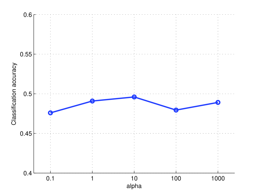
Figure 1: Sensitivity curve of $\alpha$ over PASCAL VOC 07 data set.

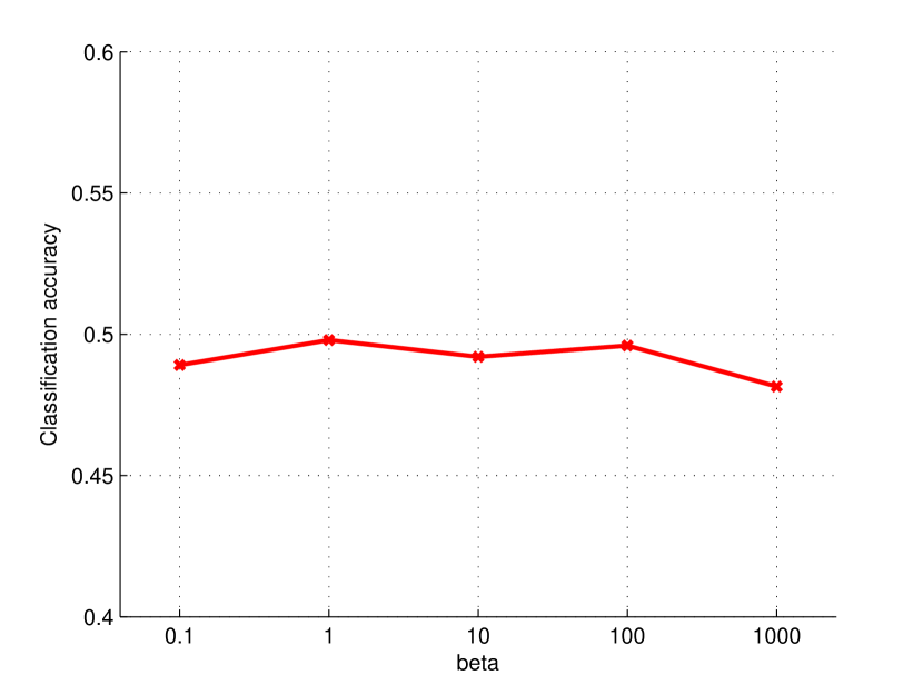
Figure 2: Sensitivity curve of $\beta$ over PASCAL VOC 07 data set.

To study the performance of the proposed algorithm with different tradeoff parameters, $\alpha$ and $\beta$. We perform the algorithm by using the parameters of values $0.1,1,10,100$ and $1000$, and measured the performance of different parameters. Fig. 1 illustrates the performance on the PASCAL VOC 07 data set with respect to different tradeoff parameter $\alpha$. The proposed algorithm achieves a stable performance in all the settings of parameter $\alpha$. In Fig. 2, the performance against different tradeoff parameter $\beta$ is also shown. From this figure, we can also see that the algorithm is stable tot he changes of value of $\beta$. This suggests that MISC is not sensitive to the changes of tradeoff parameters.

3.4.2 Comparison to state-of-the-art algorithms

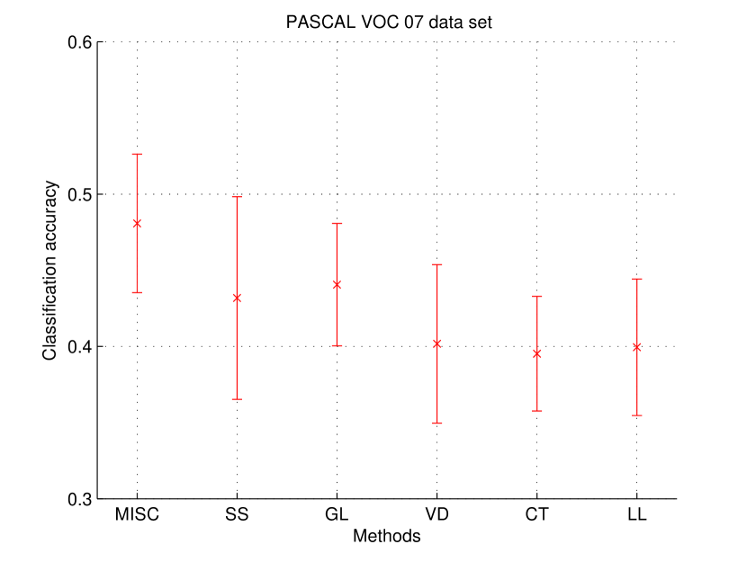
Figure 3: Results of comparison of different algorithms over PASCAL VOC’07 data set.

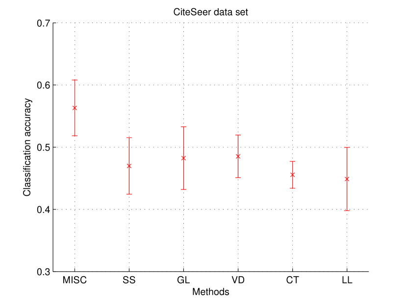
Figure 4: Results of comparison of different algorithms over CiteSeer data set.

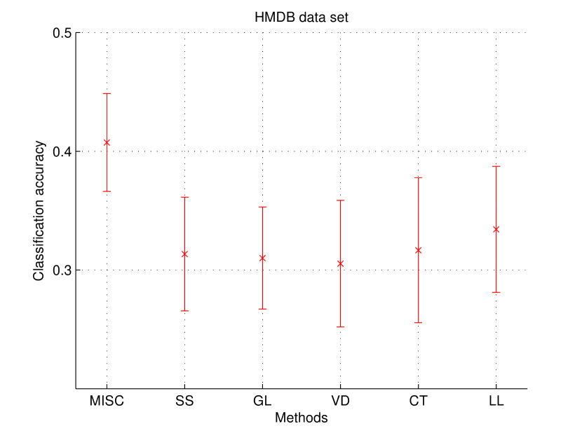
Figure 5: Results of comparison of different algorithms over HMDB data set.

We compare the proposed algorithm to the following methods, multiview learning algorithm using local learning (LL) proposed by Zhang et al. Zhang2008752 , multiview learning algorithm using co-training (CT) proposed by Sindhwani et al. sindhwani2005co , multiview learning algorithm based on view disagreement (VD) proposed by Quadrianto Quadrianto2011425 , multiview learning algorithm with global consistency and local smoothness (GL) proposed by Zhai Zhai2012 , and multiview representation method using statistical subspace learning (SS) proposed by Chen et al. Chen20122365 . The error bars of the classification accuracy of the compared methods over three different data sets are given in Fig. 3, Fig. 3 and Fig. 5. From the figures, we find that the proposed method, MISC, stably outperforms other algorithms at all the data sets. Even on the most difficult data set, HMDB, the proposed method, MISC, also achieves an accuracy as high as about 0.4. The multiple view data are optimally combined by MISC to find the latent intact space and the optimal classifier in the corresponding intact space. The main reason for this is the robust property of the proposed algorithm. This algorithm has the ability to appropriately handle the complementary between multiple views, and learn a discriminative hidden intact space with help of classifier learning.

4 Conclusions and future works

We propose a novel multiview learning algorithm by learning intact vectors of the training data points and a classifier in the intact space. The intact vectors is assumed to be a hidden but critical vector for each data point, and we can obtain its multiple view feature vectors by view-conditional transformations. Moreover, we also assume that the intact vectors are discriminative, i.e., can be separated by a linear function according to their classes. We propose a novel optimization problem to model both the learning of intact vectors and classifier. An iterative algorithm is developed to solve this problem. This algorithm outperforms other multiview learning algorithms on benchmark data sets, and it also shows its stability over tradeoff parameters. In the future, we will study the potential to use the proposed algorithm for imbalanced data set with multi-view features fan2011margin ; fan2010enhanced ; chawla2004editorial , and the usage of Bayesian network classifier instead of linear classifier to learn the intact vectors of multi-view data fan2014tightening ; fan2014finding ; fan2015improved . Moreover, we will also investigate to use the proposed algorithm to solve the problems of bioinformatics wang2014computational ; zhou2014biomarker ; liu2013structure ; peng2015modeling , computer vision wang2015representing ; wang2015image , and multi-media data processing wang2015supervised ; wang2015multiple .

References

- (1) Charuvaka, A., Rangwala, H.: Convex multi-task relationship learning using hinge loss. In: IEEE SSCI 2014 - 2014 IEEE Symposium Series on Computational Intelligence - CIDM 2014: 2014 IEEE Symposium on Computational Intelligence and Data Mining, Proceedings, pp. 63–70 (2015)
- (2) Chawla, N.V., Japkowicz, N., Kotcz, A.: Editorial: special issue on learning from imbalanced data sets. ACM Sigkdd Explorations Newsletter 6(1), 1–6 (2004)
- (3) Chen, N., Zhu, J., Sun, F., Xing, E.: Large-margin predictive latent subspace learning for multiview data analysis. IEEE Transactions on Pattern Analysis and Machine Intelligence 34(12), 2365–2378 (2012)
- (4) Chen, P.T., Chen, F., Qian, Z.: Road traffic congestion monitoring in social media with hinge-loss markov random fields. pp. 80–89 (2015). DOI 10.1109/ICDM.2014.139
- (5) Chen, Y.W., Wang, J.L., Cai, Y.Q., Du, J.X.: A method for chinese text classification based on apparent semantics and latent aspects. Journal of Ambient Intelligence and Humanized Computing 6(4), 473–480 (2015)
- (6) Fakeri-Tabrizi, A., Amini, M.R., Goutte, C., Usunier, N.: Multiview self-learning. Neurocomputing 155, 117–127 (2015)
- (7) Fan, X., Malone, B., Yuan, C.: Finding optimal bayesian network structures with constraints learned from data. In: Proceedings of the 30th Annual Conference on Uncertainty in Artificial Intelligence (UAI-14), pp. 200–209 (2014)
- (8) Fan, X., Tang, K.: Enhanced maximum auc linear classifier. In: Fuzzy Systems and Knowledge Discovery (FSKD), 2010 Seventh International Conference on, vol. 4, pp. 1540–1544. IEEE (2010)
- (9) Fan, X., Tang, K., Weise, T.: Margin-based over-sampling method for learning from imbalanced datasets. In: Advances in Knowledge Discovery and Data Mining, pp. 309–320. Springer (2011)
- (10) Fan, X., Yuan, C.: An improved lower bound for bayesian network structure learning. In: Twenty-Ninth AAAI Conference on Artificial Intelligence, pp. 2439 – 2445 (2015)
- (11) Fan, X., Yuan, C., Malone, B.: Tightening bounds for bayesian network structure learning. In: Proceedings of the 28th AAAI Conference on Artificial Intelligence, pp. 2439 – 2445 (2014)
- (12) Feng, G., Guo, J., Jing, B.Y., Sun, T.: Feature subset selection using naive bayes for text classification. Pattern Recognition Letters 65, 109–115 (2015). DOI 10.1016/j.patrec.2015.07.028
- (13) Feng, Y., Xiao, J., Zhuang, Y., Liu, X.: Adaptive unsupervised multi-view feature selection for visual concept recognition. Lecture Notes in Computer Science (including subseries Lecture Notes in Artificial Intelligence and Lecture Notes in Bioinformatics) 7724 LNCS(PART 1), 343–357 (2013)
- (14) Gallagher, C., Fisher, T., Shen, J.: A cauchy estimator test for autocorrelation. Journal of Statistical Computation and Simulation 85(6), 1264–1276 (2015)
- (15) Gui, J., Tao, D., Sun, Z., Luo, Y., You, X., Tang, Y.: Group sparse multiview patch alignment framework with view consistency for image classification. IEEE Transactions on Image Processing 23(7), 3126–3137 (2014)
- (16) Hajmohammadi, M., Ibrahim, R., Selamat, A.: Cross-lingual sentiment classification using multiple source languages in multi-view semi-supervised learning. Engineering Applications of Artificial Intelligence 36, 195–203 (2014)
- (17) Hogenboom, A., Frasincar, F., De Jong, F., Kaymak, U.: Polarity classification using structure-based vector representations of text. Decision Support Systems 74, 46–56 (2015)
- (18) Idan, M., Speyer, J.: Multivariate cauchy estimator with scalar measurement and process noises. SIAM Journal on Control and Optimization 52(2), 1108–1141 (2014)
- (19) Jaszewski, M., Parameswaran, S., Hallenborg, E., Bagnall, B.: Evaluation of maritime object detection methods for full motion video applications using the pascal voc challenge framework. In: Proceedings of SPIE - The International Society for Optical Engineering, vol. 9407, p. 94070Y (2015)
- (20) Jiang, F., Jia, L., Sheng, X., LeMieux, R.: Manifold regularization in structured output space for semi-supervised structured output prediction. Neural Computing and Applications pp. 1–10 (2015)
- (21) Jiang, Y., Liu, J., Li, Z., Lu, H.: Semi-supervised unified latent factor learning with multi-view data. Machine Vision and Applications 25(7), 1635–1645 (2014)
- (22) Koopman, B., Karimi, S., Nguyen, A., McGuire, R., Muscatello, D., Kemp, M., Truran, D., Zhang, M., Thackway, S.: Automatic classification of diseases from free-text death certificates for real-time surveillance. BMC Medical Informatics and Decision Making 15(1) (2015). DOI 10.1186/s12911-015-0174-2
- (23) Kuehne, H., Jhuang, H., Garrote, E., Poggio, T., Serre, T.: Hmdb: A large video database for human motion recognition. In: Proceedings of the IEEE International Conference on Computer Vision, pp. 2556–2563 (2011)
- (24) Kumar Nagwani, N.: A comment on ’a similarity measure for text classification and clustering’. IEEE Transactions on Knowledge and Data Engineering 27(9), 2589–2590 (2015)
- (25) La, L., Wang, N., Zhou, D.P.: Improving reading comprehension step by step using online-boost text readability classification system. Neural Computing and Applications 26(4), 929–939 (2015)
- (26) Li, X.X., Li, R.F., Feng, F.X., Cao, J., Wang, X.J.: Multi-view supervised latent dirichlet allocation. Tien Tzu Hsueh Pao/Acta Electronica Sinica 42(10), 2040–2044 (2014)
- (27) Liu, J., Jiang, Y., Li, Z., Zhou, Z.H., Lu, H.: Partially shared latent factor learning with multiview data. IEEE Transactions on Neural Networks and Learning Systems 26(6), 1233–1246 (2015)
- (28) Liu, X., Wang, J., Yin, M., Edwards, B., Xu, P.: Supervised learning of sparse context reconstruction coefficients for data representation and classification. Neural Computing and Applications pp. 1–9 (2015)
- (29) Liu, Y., Yang, J., Zhou, Y., Hu, J.: Structure design of vascular stents. Multiscale simulations and mechanics of biological materials pp. 301–317 (2013)
- (30) Long, J., Wang, L.D., Li, Z.D., Zhang, Z.P., Yang, L.: Wordnet-based lexical semantic classification for text corpus analysis. Journal of Central South University 22(5), 1833–1840 (2015)
- (31) Lu, H., Hu, Z., Gao, H.: Multiview sample classification algorithm based on l1-graph domain adaptation learning. Mathematical Problems in Engineering 2015 (2015). DOI 10.1155/2015/329753
- (32) Luo, Y., Tao, D., Xu, C., Xu, C., Liu, H., Wen, Y.: Multiview vector-valued manifold regularization for multilabel image classification. IEEE Transactions on Neural Networks and Learning Systems 24(5), 709–722 (2013)
- (33) Mala, K., Sadasivam, V., Alagappan, S.: Neural network based texture analysis of ct images for fatty and cirrhosis liver classification. Applied Soft Computing Journal 32, 80–86 (2015)
- (34) Mohanty, A., Senapati, M., Beberta, S., Lenka, S.: Texture-based features for classification of mammograms using decision tree. Neural Computing and Applications 23(3-4), 1011–1017 (2013)
- (35) Peng, B., Liu, Y., Zhou, Y., Yang, L., Zhang, G., Liu, Y.: Modeling nanoparticle targeting to a vascular surface in shear flow through diffusive particle dynamics. Nanoscale Research Letters 10(1), 235 (2015)
- (36) Petrov, N., Georgieva, A., Jordanov, I.: Self-organizing maps for texture classification. Neural Computing and Applications 22(7-8), 1499–1508 (2013)
- (37) Picard, D., Gosselin, P.H., Gaspard, M.C.: Challenges in content-based image indexing of cultural heritage collections: Support vector machine active learning with applications to text classification. IEEE Signal Processing Magazine 32(4), 95–102 (2015)
- (38) Quadrianto, N., Lampert, C.: Learning multi-view neighborhood preserving projections. pp. 425–432 (2011)
- (39) Sindhwani, V., Niyogi, P., Belkin, M.: A co-regularization approach to semi-supervised learning with multiple views. In: Proceedings of ICML workshop on learning with multiple views, pp. 74–79 (2005)
- (40) Sindhwani, V., Rosenberg, D.S.: An rkhs for multi-view learning and manifold co-regularization. In: Proceedings of the 25th international conference on Machine learning, pp. 976–983. ACM (2008)
- (41) Sublemontier, J.H.: Unsupervised collaborative boosting of clustering: An unifying framework for multi-view clustering, multiple consensus clusterings and alternative clustering (2013). DOI 10.1109/IJCNN.2013.6706911
- (42) Sun, S.: A survey of multi-view machine learning. Neural Computing and Applications 23(7-8), 2031–2038 (2013)
- (43) Wang, J., Wang, H., Zhou, Y., McDonald, N.: Multiple kernel multivariate performance learning using cutting plane algorithm. arXiv preprint arXiv:1508.06264 (2015)
- (44) Wang, J., Zhou, Y., Duan, K., Wang, J., Bensmail, H.: Supervised cross-modal factor analysis for multiple modal data classification. SMC 2015 (2015)
- (45) Wang, J., Zhou, Y., Wang, H., Yang, X., Yang, F., Peterson, A.: Image tag completion by local learning. In: Advances in Neural Networks–ISNN 2015, pp. 232–239. Springer (2015)
- (46) Wang, J., Zhou, Y., Yin, M., Chen, S., Edwards, B.: Representing data by sparse combination of contextual data points for classification. In: Advances in Neural Networks–ISNN 2015, pp. 373–381. Springer (2015)
- (47) Wang, J.J.Y., Wang, Y., Jing, B.Y., Gao, X.: Regularized maximum correntropy machine. Neurocomputing 160, 85–92 (2015)
- (48) Wang, S., Zhou, Y., Tan, J., Xu, J., Yang, J., Liu, Y.: Computational modeling of magnetic nanoparticle targeting to stent surface under high gradient field. Computational mechanics 53(3), 403–412 (2014)
- (49) Wang, Z., Sun, X., Sun, L., Huang, Y.: Multiview discriminative geometry preserving projection for image classification. The Scientific World Journal 2014 (2014). DOI 10.1155/2014/924090
- (50) Williams, K., Wu, J., Choudhury, S., Khabsa, M., Giles, C.: Scholarly big data information extraction and integration in the citeseer? digital library. In: Proceedings - International Conference on Data Engineering, pp. 68–73 (2014)
- (51) Wu, T.X., Lian, X.C., Lu, B.L.: Multi-view gender classification using symmetry of facial images. Neural Computing and Applications 21(4), 661–669 (2012)
- (52) Yadav, A., Anand, R., Dewal, M., Gupta, S.: Multiresolution local binary pattern variants based texture feature extraction techniques for efficient classification of microscopic images of hardwood species. Applied Soft Computing Journal 32, 101–112 (2015)
- (53) Yu, J., Rui, Y., Tang, Y., Tao, D.: High-order distance-based multiview stochastic learning in image classification. IEEE Transactions on Cybernetics 44(12), 2431–2442 (2014)
- (54) Zha, Z.J., Yang, Y., Tang, J., Wang, M., Chua, T.S.: Robust multiview feature learning for rgb-d image understanding. ACM Transactions on Intelligent Systems and Technology 6(2) (2015). DOI 10.1145/2735521
- (55) Zhai, D., Chang, H., Shan, S., Chen, X., Gao, W.: Multiview metric learning with global consistency and local smoothness. ACM Transactions on Intelligent Systems and Technology 3(3) (2012)
- (56) Zhang, D., Wang, F., Zhang, C., Li, T.: Multi-view local learning. In: Proceedings of the National Conference on Artificial Intelligence, vol. 2, pp. 752–757 (2008)
- (57) Zhao, X., Evans, N., Dugelay, J.L.: Unsupervised multi-view dimensionality reduction with application to audio-visual speaker retrieval. pp. 7–12 (2013)
- (58) Zhou, Y., Hu, W., Peng, B., Liu, Y.: Biomarker binding on an antibody-functionalized biosensor surface: the influence of surface properties, electric field, and coating density. The Journal of Physical Chemistry C 118(26), 14,586–14,594 (2014)