Spectral properties of near-Earth and Mars-crossing asteroids using Sloan photometry

Abstract

The nature and origin of the asteroids orbiting in near-Earth space, including those on a potentially hazardous trajectory, is of both scientific interest and practical importance. We aim here at determining the taxonomy of a large sample of near-Earth and Mars-crosser asteroids and analyze the distribution of these classes with orbit. We use this distribution to identify the source regions of near-Earth objects and to study the strength of planetary encounters to refresh asteroid surfaces. We measure the photometry of these asteroids over four filters at visible wavelengths on images taken by the Sloan Digital Sky Survey (SDSS). These colors are used to classify the asteroids into a taxonomy consistent with the widely used Bus-DeMeo taxonomy (DeMeo et al., Icarus 202, 2009) based on visible and near-infrared spectroscopy. We report here on the taxonomic classification of 206 near-Earth and 776 Mars-crosser asteroids determined from SDSS photometry, representing an increase of 40% and 663% of known taxonomy classifications in these populations. Using the source region mapper by Greenstreet et al. (Icarus, 217, 2012), we compare for the first time the taxonomic distribution among near-Earth and main-belt asteroids of similar diameters. Both distributions agree at the few percent level for the inner part of the Main Belt and we confirm this region as a main source of near-Earth objects. The effect of planetary encounters on asteroid surfaces are also studied by developing a simple model of forces acting on a surface grain during planetary encounter, which provides the minimum distance at which a close approach should occur to trigger resurfacing events. By integrating numerically the orbit of the 519 S-type and 46 Q-type asteroids in our sample back in time for 500,000 years and monitoring their encounter distance with Venus, Earth, Mars, and Jupiter, we seek to understand the conditions for resurfacing events. The population of Q-type is found to present statistically more encounters with Venus and the Earth than S-types, although both S- and Q-types present the same amount of encounters with Mars.

1 Introduction

Asteroids are the leftovers of the building blocks that accreted to form the planets in the early Solar System. They are also the progenitors of the constant influx of meteorites falling on the planets, including the Earth. Apart from the tiny sample of rock from asteroid (25 143) Itokawa brought back by the Hayabusa spacecraft (Nakamura et al. 2011), these meteorites represent our sole possibility to study in details the composition of asteroids. Identifying their source regions is crucial to determine the physical conditions and abundances in elements that reigned in the protoplanetary nebula around the young Sun (see, e.g., McSween et al. 2006). From the analysis of a bolide trajectory, it is possible to reconstruct its heliocentric orbit and to find its parent body (e.g., Gounelle et al. 2006), but such determinations have been limited to a few objects only (Rudawska et al. 2012).
Among the different dynamical classes of asteroids, the near-Earth and Mars-crosser asteroids (NEAs and MCs), whose orbits cross that of the telluric planets, form a transient population. Their typical lifetime is of a few million years only (Bottke et al. 2002; Morbidelli et al. 2002) before being ejected from the Solar System, falling into the Sun, or impacting a planet. These populations are therefore constantly replenished by asteroids from the main asteroid belt, the largest reservoir of known small bodies, between Mars and Jupiter.
The resonances between the orbits of asteroids and that of Jupiter have been long thought (Wetherill 1979; Wisdom 1983) to provide the kick in eccentricity necessary to place asteroids on planet-crossing orbits. It was later found that the secular resonance $\nu_{6}$, delimiting the inner edge of the main belt, and the 3:1 mean-motion resonance (MMR) with Jupiter, separating the inner from the middle belt, were the most effective, compared to the 5:2 resonance, for instance, which tends to eject asteroids from the solar system (see Morbidelli et al. 2002, for a review). The major role played by the $\nu_{6}$ resonance was confirmed by the comparison between the reflectance spectra of the most common meteorites, the ordinary chondrites (OCs, 80% of all meteorite falls), the dominant class in the near-Earth space, the S-type asteroids (about 65% of the observed population, Binzel et al. 2004), and the dynamical family of S-types asteroids linked with (8) Flora in the inner belt (Vernazza et al. 2008).
The NEAs also represent ideal targets for space exploration owing to their close distance from Earth. This proximity is quantified by the energy required to set a spacecraft on a rendezvous trajectory and is often expressed as $\Delta v$ (in km/s), the required change in speed. This is the reason why the first mission to an asteroid targeted the Amor (433) Eros (Veverka et al. 2000), why all the targets of sample-return missions were selected among NEAs: (25 143) Itokawa for JAXA Hayabusa (Fujiwara et al. 2006), (101 955) Bennu for NASA OSIRIS-REx (Origins-Spectral Interpretation-Resource Identification-Security-Regolith Explorer, Lauretta et al. 2011), (162 173) Ryugu for JAXA Hayabusa2 (Yano et al. 2010), and (175 706) 1996 FG3 and (341 843) 2008 EV5 for the former ESA M3/M4 candidate MarcoPolo-R (Barucci et al. 2012) and ARM (Asteroid Redirect Mission, Abell et al. 2015), and why the recent proposition for a demonstration project of an asteroid deflection by ESA, AIDA (Asteroid Impact & Deflection Assessment, Murdoch et al. 2012), targets the NEA (65 803) Didymos. This latter point, the protection from asteroid hazard, is certainly the most famous aspect of the asteroid research known to the general public, and has triggered many initiatives leading to breakthroughs in NEA discovery and characterization of their surface and physical properties (see, e.g., Binzel 2000; Stokes et al. 2000; Ostro et al. 2002; Binzel et al. 2004; Jedicke et al. 2007; Mainzer et al. 2011a; Mueller et al. 2011, among others).
In both attempting to link NEAs and MCs transient populations with their source regions and meteorites and designing a protection strategy, the study of their composition is key. Indeed, dynamical studies allows to determine relative probabilities of the origin of asteroids belonging to those populations (e.g., Bottke et al. 2002; Greenstreet et al. 2012). These links are however not sufficient, and must be ascertained by compositional similarities (Vernazza et al. 2008; Binzel et al. 2015; Reddy et al. 2015). Moreover, different compositions yield different densities and internal structure/cohesion (Carry 2012), and an asteroid on a impact trajectory with Earth of a given size will require a different energy to be deflected or destroyed according to its nature (Jutzi and Michel 2014).
Here, we aim at classifying a large number of near-Earth and Mars-crosser asteroids into broad compositional groups by using imaging archival data. We present in Section 2 the procedure we used to retrieve the photometry at visible wavelengths from the publicly available images of the Sloan Digital Sky Survey (SDSS). We describe in Section 3 how we use the SDSS photometry to classify the objects into the commonly-used Bus-DeMeo taxonomy of asteroids (DeMeo et al. 2009), following the work by DeMeo and Carry (2013). We present the results of the classification in Section 4 before discussing their implications for source regions in Section 5 and for surface rejuvenation processes in Section 6.

2 Visible photometry for the Sloan Digital Sky Survey

2.1 The Sloan Digital Sky Survey

The Sloan Digital Sky Survey (SDSS) is a wide-field imaging survey dedicated to observing galaxies and quasars at different wavelengths. From 1998 to 2009, the survey covered over 14,500 square degrees in 5 filters: u^′, g^′, r^′, i^′, z^′  (centered on 355.1, 468.6, 616.5, 748.1 and 893.1 nm), with estimated limiting magnitude of 22.0, 22.2, 22.2, 21.3, and 20.5 for 95% completeness (Ivezić et al. 2001).

2.2 The Moving Object Catalog

In the course of the survey, 471,569 moving objects were identified in the images and listed in the Moving Object Catalogue (SDSS MOC, currently in its 4th release, including observations through March 2007). Among these, 220,101 were successfully linked to 104,449 unique objects corresponding to known asteroids (Ivezić et al. 2001). The remaining 251,468 moving objects listed in the MOC corresponded to unknown asteroids at the time of the release (August 2008).
First, we keep objects assigned a number or a provisional designation only, i.e., those for which we can retrieve the orbital elements. Among these, we select the near-Earth and Mars-crossers asteroids according to the limits on their semi-major axis, perihelion, and aphelion listed in Table 1, resulting in 2071 observations of 1315 unique objects. We then remove observations that are deemed unreliable: with any apparent magnitudes greater than the limiting magnitudes reported above (Section 2.1), or any photometric uncertainty greater than 0.05. These constraints remove a large portion of the dataset (about 75%), primarily due to the larger typical error for the z^′ filter. While there is only a small subset of the sample remaining, we are assured of the quality of the data (see DeMeo and Carry 2013, for additional information on the definition of photometric cuts). Additionally, for higher errors, the ambiguity among taxonomic classes possible for an object becomes so large that the classification (Section 3) becomes essentially meaningless. In this selection process, we kept 588 observations of 353 individual asteroids from the SDSS MOC4, as listed in Table 1.

Class	a (au)		q (au)		Q (au)	MOC4	SVO-MOC	SVOgriz	SVOgri
	min.	max.	min.	max.	min.
Atens	–	1.0	–	Q${}_{\textrm{\mars}}$	0.983	–	–	10	1
Apollos	1.0	–	–	1.017	–	14	18	82	70
Amors	–	–	1.017	1.3	–	29	73	111	40
Mars-crosser	–	–	–	Q${}_{\textrm{\mars}}$	–	310	383	622	567
Total	–	–	–	–	–	353	474	825	678

Table 1: Definition of the dynamical classes of near-Earth and Mars-crosser asteroids used in present study, based on the semi-major axis (a), perihelion (q), and aphelion (Q) of their orbit. All the objects have a perihelion inward of Mars aphelion (Q${}_{\textrm{\mars}}$) at 1.666 au. The number of objects listed in the SDSS MOC4 (Section 2.2), identified in SDSS MOC4 using SkyBoT (SVO-MOC, Section 2.3), and by the SVO NEA project (Section 2.4) are also listed. See Fig. 1 for the distribution of these objects in the orbital element space.

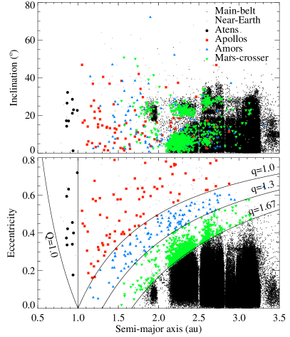
Figure 1: Distribution of the NEAs and Mars-crossers studied here as a function of their osculating elements (semi-major axis, eccentricity, and inclination). The black dots represent the first 10,000 main-belt asteroids, the grey dots the 532 NEAs with spectral classification from the literature (see Section 3.2), and the black circles, red squares, blue triangle, and green stars the Atens, Apollos, Amors, and Mars-crossers we classify from SDSS.

2.3 Identifying unknown objects in the MOC4

As mentioned above, more than half of the MOC4 entries had not been linked with known asteroids. At the time of the release (August 2008), about 460,000 asteroids had been discovered and 350,000 were numbered (i.e., had well-constrained orbits allowing easy cross-matching with SDSS detected sources). The current number of discovered asteroids has now risen above 700,000, with more than 370,000 numbered objects. We therefore use the improved current knowledge on the asteroid population to link unknown MOC sources to known objects.
We use the Virtual Observatory (VO) SkyBoT cone-search service (Berthier et al. 2006), hosted at IMCCE, for that purpose. SkyBoT pre-computes weekly the ephemeris of all known Solar System objects for the period 1889-2060, and stores their heliocentric positions with a time step of 10 days, allowing fast computation of positions at any time. The cone-search tool allows to request the list of known objects within a field of view at any given epoch as seen from Earth in typically less than 10 s. We send 251,468 requests to SkyBoT, corresponding to the 251,468 unknown objects in the MOC4, centered on the MOC4 object’s coordinates, at the reported epoch of observation, within a circular field of view of 30 arcseconds. Although many asteroids among the 700,000 known have position uncertainty larger than this value (as derived from their orbital parameter uncertainty), this cut ensures that we only keep objects with a high probability to be linked with the MOC sources.
To further restrict the number of false-positive associations, we compare the position, apparent motion, and apparent magnitude of the MOC sources to that predicted from ephemeris provided by SkyBoT, based on the database of orbital elements AstOrb. We consider successful association of SDSS sources with SkyBoT entry if the positions are closer than 30^′′, the apparent V-Johnson magnitudes do not differ by more than 0.5, and the apparent motions are co-linear (difference in $d\alpha\cos(\delta)/dt$ and $d\delta/dt$ of less than 3^′′/h). However, neither SkyBoT nor MOC4 provide estimates on the uncertainty in the apparent velocity. The only information is the uncertainty in the velocity components parallel and perpendicular to the SDSS scanning direction. The mean value of this error (both in the parallel and in the perpendicular direction) is of 1^′′/h. We are taking this value as one standard deviation to set the cut above.
Of the 251,468 unidentified MOC sources, SkyBoT provides known asteroids within 30 arcseconds for 68,497 (27%), corresponding to 41,055 unique asteroids. We trim this value to 57,646 (36,730 asteroids) for which the association can be considered certain. The vast majority of these now-identified asteroids have orbits within the main belt (35,404, corresponding to 96%), but some are NEAs (48, 0.1%), or MCs (73, 0.2%). Their respective numbers are reported in Table 1. The complete list of MOC entries associated to known asteroids (277,747 entries associated to 141,388 asteroids) is freely accessible.

2.4 The SVO Near-Earth Asteroids Recovery Program

In addition, we search the images of the SDSS for NEAs and MCs that were either not identified as moving objects by the automatic SDSS pipeline, rejected by the MOC data selection, or imaged after the latest compilation of the SDSS MOC4 (i.e., observed after March 2007). Indeed, only moving objects with an apparent motion between 0.05 and 0.050 deg/day were included in the MOC, leaving a significant fraction of NEAs un-cataloged (Solano et al. 2013).
We use the resources of the citizen-science project “Near-Earth Asteroids Recovery Program” of the Spanish Virtual Observatory (SVO) which was originally designed for this very purpose: to identify and measure the astrometry of NEAs in archival imaging data (Solano et al. 2013). For each Aten, Amor, Apollo, and Mars-crosser listed by the Minor Planet Center (MPC), its ephemeris are computed over the period of operation of the SDSS imaging survey (1998 to 2009) and compared to the footprints of the images of the survey. The images possibly containing an object brighter than the SDSS limiting magnitude (V = 22) are then proposed to the public for identification through a web portal. Since the beginning of the project in 2011, over 2,500 astrometry measurements of about 600 NEAs not identified in the MOC have been reported to the MPC (see Solano et al. 2013, for details on the project).
To compute the photometry of the NEAs measured by the users we first searched in the photometric catalog of the 8th SDSS Data Release. If no photometry associated with the NEA was found, we ran SExtractor on the corresponding images and calibrated the SExtractor magnitudes by comparing them with the SDSS magnitudes of the sources identified in the image.
Owing to the more stringent limiting magnitude in the z^′ filter, many asteroids are identified over three bands (g^′r^′i^′) only. We also report these objects here, although deriving a taxonomic classification is of course less accurate. Overall, we collect 1194 four bands (g^′r^′i^′z^′) photometry measurements of 825 unique asteroids and 976 three-bands (g^′r^′i^′) photometry measurements of 678 distinct asteroids (Table 1). We present in Fig. 2 a comparison of our measurements with the magnitudes reported in the SDSS MOC4 for the common asteroids in both sets, showing excellent agreement (values agree with a standard deviation of 0.05 mag).

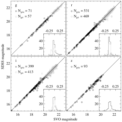
Figure 2: Comparison of the apparent magnitude measured by our system (SVO magnitude) with that reported in the SDSS MOC4 (SDSS magnitude) for the four g^′, r^′, i^′, and z^′ filters. For each, the number of common objects is reported, for both four-bands (black circles) and three-bands (grey squares) sets. The inserted histograms show the distribution of the magnitude difference (MOC-SVO)

3 Taxonomic classification

The SDSS photometry has been used to classify asteroids according to their colors by many authors (e.g., Ivezić et al. 2002; Nesvorný et al. 2005; Parker et al. 2008; Carvano et al. 2010). One key advantage of the survey was the almost simultaneous acquisition of all filters (5 min in total), hence limiting the impact of geometry-related lightcurve on the apparent magnitude. Here we follow the work by DeMeo and Carry (2013, 2014) in which the class definitions are set to be as consistent as possible with previous spectral taxonomies based on higher spectral resolution and larger wavelength coverage data sets, specifically Bus and Bus-DeMeo taxonomies (Bus and Binzel 2002; DeMeo et al. 2009). We present concisely the classification scheme below and refer to DeMeo and Carry (2013) for a complete description.

3.1 From SDSS to Bus-DeMeo taxonomy

First, we convert the photometry into reflectance (using solar colors from Holmberg et al. 2006) and normalize them to unity in filter g^′. Second, we compute the slope of the continuum over the g^′, r^′, and i^′ filters (hereafter gri-slope), and the z^′$-$i^′ color (hereafter zi-color), representing the band depth of a potential 1 $\mu$m band, because they are the most characteristic spectral distinguishers in all major taxonomies (beginning with Chapman et al. 1975). The classification into the taxonomy is then based on these two parameters.
As a results of the limited spectral resolution and range of SDSS photometry, we group together certain classes into broader complexes (see correspondences in Table 2). For asteroids with multiple observations that fall under multiple classifications, we use the tree-like selection to assign a final class (see DeMeo and Carry (2013) for details and DeMeo et al. (2014a) for an example of a spectroscopic confirmation campaign of the SDSS classification used here). We successfully classify 982 asteroids from the sample of 1015 near-Earth and Mars-crosser asteroids with four-bands photometry (i.e., 97% of the sample).
For objects with three-bands photometry only, we set their z^′ magnitude to the limiting magnitude of 20.5 (Ivezić et al. 2001) as an upper limit for their brightness. We then classify these asteroids using the scheme presented above. Because the magnitude of 20.5 in z^′ is an upper limit, the actual zi-color for these asteroids may be overestimated. The classification can therefore be degenerated, all the classes with similar gri-slope and lower zi-color being possible. We assign tentative classification to 254 asteroids from the sample of 678 near-Earth and Mars-crosser asteroids with three-bands photometry (i.e., 37% of the sample).
In all cases, we mark objects with peculiar spectral behavior with the historical notation “U” (for unclassified), and discard them from the analysis. There are 33 and 424 asteroids in the four-bands and three-bands photometry samples respectively for which we cannot assign a class. These figures highlight the ambiguity raised by the lack of information on the presence or absence of an absorption band around one micron, to which the z^′ filter is sensitive.

3.2 Gathering classifications from past studies

Many different authors have reported on the taxonomic classification of NEAs. We gather here the results of Dandy et al. (2003), Binzel et al. (2004), Lazzarin et al. (2005), de León et al. (2006), de León et al. (2010), Thomas and Binzel (2010), Popescu et al. (2011), Ye (2011), Reddy et al. (2011), Polishook et al. (2012), Sanchez et al. (2013), and DeMeo et al. (2014b). These authors used different taxonomic schemes to classify their observations, using either broad-band filter photometry or spectroscopy, at visible wavelengths only or also in the near infrared. We therefore transpose the classes of these different schemes (Tholen 1984; Tholen and Barucci 1989; Bus and Binzel 2002; DeMeo et al. 2009) into the single, consistent, set of 10 classes we already use for the SDSS data. Here also, we attribute the historical “U” designation for objects with apparently contradictory classifications (e.g., QX or STD in Ye 2011). These pathological cases represent 15% of the objects with multiple class determinations. In total, we gather 1022 classifications for 648 objects listed in the literature.

SDSS & Literature	Bus-DeMeo
A, AR, AS	A
B	B
C, C:, Cb, Cg, Ch	C
D, DT	D
K, K:	K
L, Ld	L
Q, Q/R, R, RQ	Q
O, Q/R/S, R, RS	S
S, S:, S(I$\rightarrow$V), Sa, Sk, Sl, Sq, Sq:, Sr	S
V, V:	V
E, M, P, X, X:, XT, Xc, Xe, Xk	X
U, C(u), R(u), S(u), ST, STD, QX	U

Table 2: Correspondence between the classes from different taxonomies (e.g., Tholen and Barucci 1989; Bus and Binzel 2002) found in the literature, used to classify the SDSS photometry (in bold), and their equivalence in the reduced version of the taxonomy by DeMeo et al. (2009) adopted here, following the work by DeMeo and Carry (2013). We strive to preserve the most extreme classes (like A, B) and we convert the tentative classification (e.g., RS) into their broader, safer, complex (S). We also consider as unknown (U) any data of insufficient quality.

4 Results

We list in Table B the photometry and the taxonomy of all 982 near-Earth and Mars-crossers asteroids with four-bands photometry. The 254 asteroids with three-bands photometry are listed separately in Table B, because their taxonomic classification is less robust. In many cases, the upper limit of 20.5 for their z^′ magnitude provides a weak constraint on their taxonomy, and classes with high zi-color (mainly V-types) are more easily identified. This sample based on three-bands photometry only is therefore biased, but it can be used as a guideline for selecting targets for spectroscopic follow-ups. We concentrate below on the sample based on four-bands photometry.
The 206 NEAs presented here have absolute magnitudes between 12 and 23. Our sample fully overlaps with the size range of the 523 NEAs characterized by visible/near-infrared spectroscopy published to date and represents an increase of $\approx$40% of the current sample size (Fig. 3). A significant fraction (46%) of the NEA population with H $<$ 16 (about 2 km diameter for an albedo of 0.20) has a taxonomic classification. For smaller diameters, the fraction drops quickly to 10% and less. The sub-kilometer population of NEAs is therefore still poorly categorized.
The absolute magnitude of the 776 MCs reported here ranges from 11 to 19. Our sample represents the first classification of sub-kilometric Mars-crossers, and a sixfold increase to the sample of 117 MCs from spectroscopy (Fig. 3). Similarly to NEAs, about 40% of the MC population with H $<$ 14 (about 5 km diameter for an albedo of 0.20) now has a taxonomic classification, and the fraction drops quickly to 10% for smaller diameters.

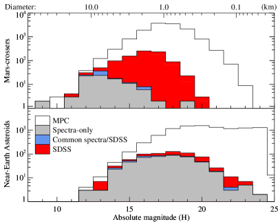
Figure 3: Distribution of the known taxonomy for near-Earth and Mars-crosser asteroids as a function of their absolute magnitude H. The white histogram corresponds to the total number of discoveries (listed in AstOrb), the grey to the taxonomic classification found in the literature, the blue to the overlap between literature and present study, and the red the four-bands set. An approximative conversion to diameter is also reported, using $D=1329\times p_{v}^{-0.5}\times 10^{-0.2H}$, with the geometric albedo $p_{v}$ taken as 0.2 (the majority, $\approx$60%, of the objects classified here being S-types).

4.1 Taxonomy and orbital classes

We present in Fig. 4 how the different classes distribute among the orbital populations. As already reported by Binzel et al. (2004), the broad S- (including Q-types), C-, X-complexes, and V-types dominate the NEA population, the minor classes (A, B, D, K, L) accounting for a few percents only, similarly to what is found in the inner main belt (DeMeo and Carry 2013, 2014). We find that the S-complex encompasses twice as many objects as the C- and X-complexes, compared to the threefold difference reported by Binzel et al. (2004).
The distribution of taxonomic classes among MCs is similar to that of Apollos and Amors (with only 8 Atens, our sample suffers from low-number statistics). Our findings of V-types accounting for roughly 5% of all MCs may therefore seem puzzling considering the lack of V-types among the $\approx$100 classified MCs highlighted by Binzel et al. (2004). It is, however, an observation selection effect. Indeed, Mars-crossers are inner-main belt (IMB) asteroids which eccentricity has been increased by numerous weak mean-motion resonances (“chaotic diffusion”, see Morbidelli and Nesvorný 1999). The IMB hosting the largest reservoir of V-types in the solar system (Vestoids, Binzel and Xu 1993), V-types were expected in MC space.
The size distribution of known Vestoids however peaks at H = 16 (about 1.5 km diameter), and the largest members have an absolute magnitude of 14 (we use the list of Vestoids from Nesvorny 2012). All the V-types identified here have an absolute magnitude above 14, and so does (31 415) 1999 AK23 (H = 14.4), the first V-type among MCs reported recently by Ribeiro et al. (2014). Only 33 MCs had been characterized with this absolute magnitude or higher to date, and the previous lack of report of V-types among MCs is consistent with our findings.

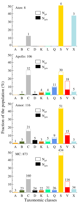
Figure 4: Distribution of the taxonomic classes for each dynamical group: Aten, Apollo, Amor, and Mars-crosser. The number of object with four-band photometry in each class is reported. Empty and filled bars stands for the three and four band photometry samples respectively.

4.2 Low-$\delta v$ as space mission targets

Within the 206 NEA serendipitously observed by the SDSS, we identify 36 potential targets for space missions based on their accessibility. We select all the NEA with a $\delta v$ below 6.5 km/s. As a matter of comparison, the required $\delta v$ to reach the Moon and Mars are of 6.0 and 6.3 km/s (e.g., Abell et al. 2012). We list in Table 3 the basic characteristics of these potential targets, together with the targets already, or planned to be, visited by spacecraft.
Among the list of low-$\delta v$ objects, we find a large majority of S-types, following their dominance in the sample presented here of about 60%. We, however, note the presence of potential D-, L-, and K-types. To date, of the 24 taxonomic classes, only C- (Mathilde, Ceres), S- (Ida, Eros, Gaspra, Itokawa, and Toutatis), Xe- (Steins), Xk- (Lutetia), and V-types (Vesta) have been visited by spacecraft. These potential D-, L-, and K-types targets may represent good opportunities for exploration. Data in the visible can only suggest the presence of an absorption band at 1 $\mu$m, and near-infrared data is required to confirm these potential classifications.

Designation	Type	Class	$\delta v$ (km/s)	H	$s$ (%/100 nm)	z-i	a (au)	e	i (${}^{\textrm{o}}$)
2004 EU22	X	Apollo	4.420	23.00	0.78	0.044	1.175	0.162	5.3
1996 XB27	D	Amor	4.750	22.00	0.85	0.123	1.189	0.058	2.5
2000 TL1	C	Apollo	4.870	22.00	-0.09	0.002	1.338	0.300	3.6
2001 QC34	Q	Apollo	4.970	20.00	0.69	-0.228	1.128	0.187	6.2
1999 FN19	S	Apollo	5.020	22.00	0.96	-0.135	1.646	0.391	2.3
2000 SL10	Q	Apollo	5.080	21.00	0.86	-0.189	1.372	0.339	1.5
1994 CN2	S	Apollo	5.150	16.00	1.12	-0.073	1.573	0.395	1.4
2002 LJ3	S	Amor	5.280	18.00	1.07	-0.258	1.462	0.275	7.6
2004 UR	C	Apollo	5.320	22.00	0.13	-0.025	1.559	0.406	2.4
2006 UP	S	Amor	5.350	23.00	1.43	-0.074	1.586	0.301	2.3
1994 CC	S	Apollo	5.370	17.00	0.99	-0.210	1.638	0.417	4.7
2010 WY8	K	Amor	5.670	21.00	0.92	-0.042	1.385	0.136	6.0
2002 XP40	S	Amor	5.720	19.00	1.63	-0.092	1.645	0.296	3.8
1993 QA	D	Apollo	5.740	18.00	1.02	0.174	1.476	0.315	12.6
2004 RK9	C	Amor	5.760	21.00	0.14	-0.050	1.837	0.426	6.2
2001 FC7	C	Amor	5.780	18.00	0.16	-0.034	1.436	0.115	2.6
1977 VA	C	Amor	5.940	19.20	0.34	-0.010	1.866	0.394	3.0
2001 WL15	C	Amor	6.000	18.00	0.34	-0.179	1.989	0.475	6.9
2000 XK44	L	Amor	6.080	18.00	1.24	0.020	1.724	0.385	11.2
2003 BH	V	Apollo	6.090	20.00	1.79	-0.273	1.456	0.356	13.1
2000 NG11	X	Amor	6.130	17.00	0.27	0.089	1.881	0.368	0.8
2000 RW37	C	Apollo	6.150	20.00	0.45	-0.166	1.248	0.250	13.8
2001 FD90	V	Amor	6.200	19.00	0.75	-0.419	2.046	0.478	7.3
2002 PG80	S	Amor	6.210	18.00	1.09	-0.225	2.013	0.438	4.4
2004 VB	S	Apollo	6.260	20.00	1.04	-0.200	1.458	0.409	10.9
1993 DQ1	S	Amor	6.270	16.00	1.20	-0.207	2.036	0.493	10.0
2000 YG4	Q	Amor	6.300	20.00	0.61	-0.155	2.211	0.503	2.6
2004 KD1	C	Amor	6.330	17.00	0.13	-0.110	1.720	0.331	10.1
2004 RS25	C	Amor	6.410	20.00	0.39	-0.057	2.128	0.479	6.7
2004 QZ2	S	Amor	6.470	18.00	-5.74	-0.227	2.260	0.495	1.0
2001 FY	S	Amor	6.530	18.00	1.36	-0.132	1.886	0.327	4.7
2009 OC	S	Amor	6.540	20.00	0.85	-0.153	2.137	0.446	4.6
2004 XM35	S	Amor	6.560	19.00	1.13	-0.111	1.837	0.301	5.4
2005 QG88	K	Apollo	6.560	20.00	0.99	-0.056	1.728	0.493	11.3
1999 KX4	V	Amor	6.580	16.00	1.60	-0.432	1.457	0.293	16.6
2002 TY57	S	Amor	6.600	19.00	0.86	-0.154	1.922	0.327	3.5
Itokawa	S	Apollo	4.632	19.20			1.324	0.280	1.6
Bennu	C	Apollo	5.087	20.81			1.126	0.204	6.0
Ryugu	B	Apollo	4.646	19.17			1.189	0.190	5.9
Didymos	X	Apollo	5.098	17.94			1.644	0.384	3.4

Table 3: List of NEAs with a low $\delta v$, hence potential targets for space missions. For each NEA, the taxonomic class determined here is reported, together with the dynamical class, the absolute magnitude and the orbital elements. The targets of the asteroid-deflection mission AIDA (Didymos) and of the return-sample missions Hayabusa (Itokawa), OSIRIS-REx (Bennu), and Hayabusa2 (Ryugu) are also included for comparison.

5 Source regions

The population of NEAs being eroded on short timescale ($<$ 10 My) by planetary collisions and dynamical ejections, new objects must be injected in the NEA space to explain the current observed population. We use our sample of 982 NEAs and MCs to identify possible source regions. For that, we use the source region mapper by Greenstreet et al. (2012), built on the result of numerical simulations of the orbital evolution of test particules in the five regions defined by Bottke et al. (2002): $\nu_{6}$ secular resonance, 3:1 mean-motion resonance with Jupiter, Mars-crossers (MC), Outer Belt (OB), and Jupiter Family Comet (JFC).
For each object, we compute its probability $\mathcal{P}_{i}$ to originate from the $i^{\textrm{th}}$ source region. We then normalize all $\mathcal{P}_{i}$ for each source region. The sum of the normalized $\mathcal{P}_{i}$ over a given taxonomic class therefore represents the fraction of objects (by number) of this class in the source region (Table 4). Uncertainties are computed from the source region mapper uncertainties, quadratically added with the margin of error (at 95% confidence level) to account for the sample size. We can then compare these predicted fractions to the observed distribution of taxonomic classes for each source region.
The vast majority of NEAs with taxonomic classification sustain diameters of less than 5 km (absolute magnitude above 14). Because the distribution of taxonomic classes in the main belt varies with diameter (DeMeo and Carry 2014), we need to compare the predicted fraction of Table 4 with objects with H $>$ 14 in each source region. For the first time, thanks to the large dataset of asteroids provided by the Sloan Digital Sky Survey (SDSS), such information is available for the inner part of the main belt (DeMeo and Carry 2013, 2014) and is reported in Table 4 (3 to 5 km diameter range).
The comparison of the $\nu_{6}$ and 3:1 source regions (delimiting the inner belt) with the observations in Fig. 5 shows a very good match of the distributions (correlation coefficient of 0.99, maximum difference of 5%). This validates the dynamical path from the inner belt to the near-Earth space as described in the model by Greenstreet et al. (2012). Although the inner belt is widely accepted as a major source for NEAs and meteorites (e.g., Bottke et al. 2002; Binzel et al. 2004; Vernazza et al. 2008; Binzel et al. 2015), the relative contribution of the different source regions particularly with respect to asteroid size is still a matter of debate. For the first time, we compare here populations of the same size range.

Class	Source regions										IMB${}_{\rm 3-5\,km}$
	MC		$\nu_{6}$		MMR3:1		OB		JFC		(#)	(%)
A	0.4 $\pm$	5.9	0.5 $\pm$	6.3	0.3 $\pm$	5.5	0.0 $\pm$	3.0	0.0 $\pm$	3.0	9	0.4
B	2.4 $\pm$	5.8	1.7 $\pm$	5.4	2.9 $\pm$	6.1	6.1 $\pm$	7.5	0.4 $\pm$	4.3	34	1.5
C	15.7 $\pm$	5.2	20.5 $\pm$	5.4	22.7 $\pm$	5.6	38.6 $\pm$	6.6	47.3 $\pm$	10.6	589	25.7
D	2.5 $\pm$	5.7	2.3 $\pm$	5.6	2.5 $\pm$	5.8	5.8 $\pm$	7.2	9.7 $\pm$	8.5	20	0.9
K	2.8 $\pm$	5.9	2.5 $\pm$	5.8	2.4 $\pm$	5.7	4.8 $\pm$	6.9	1.8 $\pm$	7.3	57	2.5
L	3.8 $\pm$	5.9	3.4 $\pm$	5.7	4.4 $\pm$	6.1	1.9 $\pm$	5.1	0.4 $\pm$	4.2	73	3.2
Q	3.6 $\pm$	5.6	4.3 $\pm$	5.8	6.3 $\pm$	6.4	3.8 $\pm$	5.8	2.4 $\pm$	5.5	0	0.0
S	52.8 $\pm$	4.6	44.5 $\pm$	4.6	42.0 $\pm$	4.8	23.8 $\pm$	4.8	23.4 $\pm$	6.9	1145	50.0
V	13.0 $\pm$	5.5	15.6 $\pm$	5.7	12.5 $\pm$	5.5	7.0 $\pm$	5.0	3.0 $\pm$	4.7	247	10.8
X	3.2 $\pm$	5.5	4.7 $\pm$	6.0	4.0 $\pm$	5.8	8.1 $\pm$	7.2	11.7 $\pm$	10.3	117	5.1

Table 4: Relative fraction of each taxonomic class (by number of objects) from each source region defined by Bottke et al. (2002) and Greenstreet et al. (2012), compared with the distribution of taxonomic types among 3 to 5 km inner Main Belt (IMB) asteroids (where Q-types are merged with S-types, see DeMeo and Carry 2013).

Unfortunately, there is no similar data set for the other source regions (MC, OB, and JFC) to be compared with our prediction. We can still note the overall trend of increasing fraction of C/D/X-types in OB and JFC compared with the inner regions, as expected. The fraction of K-types peaks in the outer belt, place of the Eos family, also as expected, although a steady distribution of K-types across source regions is also consistent within uncertainties. We also note a strong correlation between MC and small inner-belt asteroid populations (correlation coefficient 0.97), which is not related to the origin of NEAs, but of MC themselves, via chaotic diffusion from the inner belt (see Morbidelli and Nesvorný 1999; Michel et al. 2000).
A peculiar feature of Table 4 is the high fraction of S-type in all source regions. Based on present set of NEAs and the dynamical model by Greenstreet et al. (2012), one asteroid below 5 km diameter out of four should be an S-type in the outer belt and the same applies to Jupiter family comets. Although the census of composition in this size range (3–5 km) is far from being complete in these regions, there is a bias toward detecting S-types due to their high albedo ($\approx$0.20) compared to that of the C/P/D-types found there (around 0.05, see Mainzer et al. 2011b; DeMeo and Carry 2013, for albedo averages over taxonomic classes) S-types are minor contributors to the outer belt for diameters above 5 km (DeMeo and Carry 2014) and searches for S-type material have been unsuccessful among Cybeles, Hildas, and Trojans (see Emery and Brown 2003, 2004; Emery et al. 2011; Fornasier et al. 2004, 2007; Yang and Jewitt 2007, 2011; Roig et al. 2008; Gil-Hutton and Brunini 2008; Marsset et al. 2014). However, only 4% of the sample (42 objects) are predicted to originate from the OB and JFC source regions. The results for these regions is, thus, based on small number statistics. The large fraction of S-types in these source regions suggests nevertheless that dynamical models may require further refinements.

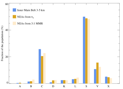
Figure 5: Relative fractions (by number) of taxonomic classes for asteroids in the inner part of the main-belt (2.0–2.5 au) with diameter between 3 and 5 km (computed from DeMeo and Carry 2013, 2014) compared with the predicted fractions originating from $\nu_{6}$ and 3:1 resonances (see Sec. 5)

6 Spectral slope and space weathering

6.1 Size dependence of spectral slope

A size dependency of the spectral characteristics of S-type asteroids has been detected early on (e.g., Gaffey et al. 1993) and a correlation between size and spectral slope among NEAs and MCs was shown by Binzel et al. (2004) based on a sample of 187 S- and 20 Q-types. Independently of the other reddening effects due to grain size (see, e.g., Cloutis et al. 2015) and solar phase angle (Bell et al. 2002; Sanchez et al. 2012; Reddy et al. 2015), this trend has been associated with space weathering, causing the spectrum of Q-types, i.e., that of ordinary chondrites made of assemblage of olivine and pyroxenes, to redden into S-type spectra under the action of solar wind ions (see Sasaki et al. 2001; Strazzulla et al. 2005, among many others). Even if the timescale of this reddening is still debated (from $<10^{6}$ yrs by, e.g., Vernazza et al. (2009) to more than $10^{9}$ yrs by, e.g., Willman and Jedicke (2011)), it is shorter than the age of the Solar System (see also Jedicke et al. 2004; Nesvorný et al. 2005; Willman et al. 2008, 2010; Dell’Oro et al. 2011; Marchi et al. 2010, 2012). Some regolith refreshing mechanisms must therefore be invoked to explain non- and less-weathered surfaces.
Because the collisional lifetime decreases with size, the surface is expected to be younger at smaller sizes. Smaller asteroids should therefore have a shallower spectral slope than larger bodies on average, albeit with a larger dispersion as collisions are a stochastic process (Binzel et al. 2004). This trend has been found recently for the small (diameter below 5 km) members of the Koronis family in the main belt ($\approx$400 objects, Rivkin et al. 2011; Thomas et al. 2011, 2012). We present in Fig. 6 the spectral slope of 467 S-types plotted against their absolute magnitude. This sample is almost 3 times bigger than that of Binzel et al. (2004), and although we cannot directly compare the values of the spectral slope due to the different definitions and normalization wavelength, we note that we observe the same linear trend from 5 to 1 km (also visible in Thomas et al. 2012). However, we do not observe an increase of the standard deviation toward smaller diameters nor a “saturation” regime below 1 km as visible in their Fig. 7. If this trend seems to persist below 1 km, the statistical relevance of this information decreases, however, as the number of objects drops dramatically, both here and in Binzel et al. (2004).
We interpret the difference between our findings and those reported by Binzel et al. (2004) as the effect of the larger sample, in which the signal to noise ratio of the data is roughly constant over the entire size range: contrarily to the spectral observations, generally noisier for small objects, the limiting factor of the present SDSS data is the apparent z^′ magnitude. Objects with four-bands photometry were brighter than magnitude 20 at the time of their observations, that is 2 magnitudes brighter than the limiting magnitude in g^′, r^′, and i^′, over which the spectral slope is computed.
Perhaps not surprisingly, a similar trend is visible for the 38 Q-types displayed in Fig. 6. These represent the youngest surfaces of their size range. Following the argument above, larger asteroids are refreshed less often than smaller objects, and this also applies to Q-types on their path to redden into S-types, independently of the mechanism that originally reset their surface.

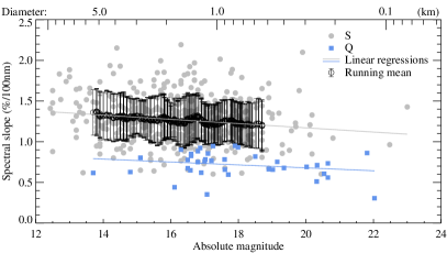
Figure 6: Spectral slope of 467 S- and 38 Q-types against their absolute magnitude (H). An approximative conversion to diameter is also reported (see Fig. 3). For both, a linear regression is presented, together with a running-window average (window size 50) for the sample of S-types.

6.2 Planetary encounters refresh surfaces

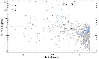
Figure 7: Absolute magnitude of S- and Q-types asteroids against perihelion distance. Below H = 18 (95% of our MC sample), the Q/S fraction among NEAs and MCs is roughly similar (5–8%). The Q/S fraction rapidly increase for smaller diameters (H $>$ 18) among NEAs, and many Q-types will be discovered in the sub-kilometer population of MCs.

If collisions play a stochastic role in modulating the spectral slope of silicate-rich asteroids (S-, A-, V-, Q-types), the question on the main rejuvenating process is still open. Binzel et al. (2010) and DeMeo et al. (2014b) have recently provided observational support to the mechanism proposed by Nesvorný et al. (2005) of close encounters with terrestrial planets. The tidal stress during the close encounters has been proposed to reveal fresh material (responsible for the Q-type appearance) via landslides and regolith shaking.
Both Binzel et al. (2010) and DeMeo et al. (2014b) investigated the orbital history of two samples of near-Earth Q- and S-type asteroids, searching for planetary encounters “close enough” (up to a few lunar distances) to reset space weathering effect. As a results, all the Q-types they tracked had small MOID with either the Earth or Mars in the past 500,000 years, a time at which some level of space weathering should have already developed (see Sect. 6.1 above). A significant fraction of S-types had also small MOIDs with terrestrial planets. However, the MOID measures the distance between two orbits, and not between two bodies, and a small MOID does not necessarily implies encounters. The authors concluded that planetary encounters, with Mars and the Earth, could explain the presence of Q-types among NEAs (while they are rare among main-belt asteroids). They derived a putative range $r^{\star}$ of 16 Earth radii at which the resurfacing could be felt by asteroids.
Independently, Nesvorný et al. (2010) used the sample by Binzel et al. (2010), using a different approach. By tracking test particles from NEA source regions (similar to Bottke et al. 2002, in a way) to NEA space and using a simple step-function model for space weathering, they explored the possible range of planetary distances and space weathering timescales that would result in the amount and orbital distribution of the Q/S ratio. They concluded on a smaller sphere of influence of planets, with $r^{\star}$ between 5 and 10 Earth radii. Contrarily to Binzel et al. (2010), who only addressed Earth encounters, they found encounters with Venus were as effective as those with the Earth. They finally found that encounters with Mars were less important, and predicted a very small fraction of Q-types among Mars-crossers ($\lesssim$1%).
The 23 Q-types candidates we identified among Mars-crossers (Sec. 4) account for about 2.5% of the sample (and the Q/S ratio is about 5%). This ratio is smaller than for NEAs where it reaches 20% (the total fraction of Q-types among NEAs is 8%), but it is a lower limit. The Q/S fraction is indeed strongly diameter-dependent as illustrated in Fig. 7. When comparing similar size range (H $<$ 18, corresponding to 95% of the MC sample here), the Q/S fraction is roughly similar for NEAs and MCs, around 5–8%. The ratio jumps to 40% for sub-kilometric NEAs, and many more Q-types could be discovered among sub-kilometric MCs. Because of this high fraction of Q-types among MCs, challenging the prediction by Nesvorný et al. (2010), we first derive the theoretical radius of influence during an planetary encounter by studying the forces acting on surface grains (Sec. 6.2.1 to Sec. 6.2.4) and then study the dynamical history of all the S- and Q-types asteroids presented here, recording their close encounters with massive bodies (Sec. 6.2.5).

6.2.1 Resurfacing model

While resurfacing of asteroids by planetary encounters has already been studied (Nesvorný et al. 2005, 2010; Binzel et al. 2010; DeMeo et al. 2014b), the physics of the surface was not given much attention in the aforementioned articles. The velocity and duration of the encounter, the object’s shape, internal structure, surface gravity, local slopes, rotation rate and orientation, and the nature of the pre-existing regolith and its cohesion, were listed as possible parameters dictating the distance at which an encounter can resurface the asteroid.
In the following we are interested in finding the mean processes responsible for resurfacing and the minimum close encounter distances at which it would occur. We thus consider a simple force balance equation describing the accelerations a surface particle is likely to experience at the moment of closest approach. A particle on the asteroid’s surface is subject to the following forces during a flyby (e.g., Hartzell and Scheeres 2011) :

$$F_{td}+F_{cf}+F_{es}+F_{lt}=F_{ga}+F_{co}+F_{sp}$$ (1)

On the left-hand side of equation (1) we have summed all the forces that can displace the particle: $F_{td}$ are the tidal forces due to the planetary encounter, $F_{cf}$ is the centrifugal pseudo force due to the asteroid’s rotation, $F_{es}$ is a repulsive electrostatic force that originates from the electric charging of surface particles, and $F_{lt}$ is the displacement force acting when the asteroid’s rotation state changes (librational transport, see Yu et al. 2014). The right-hand side contains forces that can keep a particle in place: $F_{ga}$ is the self-gravity of the asteroid, $F_{co}$ is the cohesion between surface particles, and $F_{sp}$ is the solar radiation pressure. We describe the force model in detail in A and show in Fig. 8 their absolute magnitude as function of the diameter of surface grains.

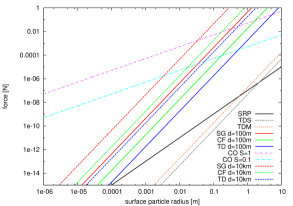
Figure 8: Comparison of the forces acting on surface particles as function of their diameter during an encounter with the Earth at a 10 Earth-radii distance. The different lines represent the absolute magnitude of the following forces: self gravity (SG), cohesion (CO), centrifugal forces (CF), solar radiation pressure (SRP) for two different asteroid diameters, 100 m and 10 km, with the same bulk density (1900 kg.m^-3) and rotation period ($P$ = 10 h). Tidal accelerations due to the moon (TDM) and the sun (TDS) are only visible for the asteroid with a 100 m diameter. The range of likely cohesive forces is represented by the choice of cleanliness parameters between 0.1 and 1 (Perko et al. 2001; Scheeres et al. 2010; Hartzell and Scheeres 2011; Sánchez and Scheeres 2014). One can see that cohesion dominates all other forces for particle sizes below $10^{-3}$ m.

To determine the minimum planet-to-asteroid distances that would result in the resurfacing of the asteroid, we consider two limiting cases (see Fig. 9). Easy and hard cases are defined based on whether the conditions for resurfacing are favorable or not, respectively. By doing so, we aim at deriving limits to distinguish regions in the parameter space where resurfacing is practically guaranteed, from regions that will leave the asteroid’s surface untouched.

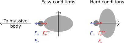
Figure 9: Schematic view of the easy (6.2.2) and hard (6.2.3) conditions for resurfacing. The forces acting on a surface particles are: $F_{td}$ are the tidal forces due to the planetary encounter, $F_{cf}$ is the centrifugal force due to the asteroid’s rotation, $F_{ga}$ is the self-gravity of the asteroid, and $F_{co}$ is the cohesion between surface particles.

6.2.2 Easy resurfacing conditions

If the asteroid has a rotation rate close to the spin-barrier and it passes the planet with its spin axis perpendicular to the orbital plane of the hyperbolic encounter, i.e., with zero obliquity with respect to the planet, resurfacing is more likely. Since fast rotators are stable with regard to perturbations of the spin state, we can assume that the initial spin vector remains constant and librational transport will not play a role. Low self-gravity is also conducive to resurfacing. The effect of solar radiation pressure can be neglected, because it is orders of magnitude weaker than the other contributions.
Considering the high porosity of the first layers of asteroid surfaces Vernazza et al. (2012) that could originate from the electrostatic charging of the surface particles, we deem cohesion between surface particles to be negligible in this case. Since electrostatic inter-particle repulsion is already incorporated in the assumption of a highly porous upper layer of regolith, no additional electrostatic forces shall be considered. As a consequence of the above assumptions that yield the best case scenario in terms of resurfacing an asteroid, equation (1) simplifies to

$$F_{td}+F_{cf}^{max}=F_{ga}^{min}$$ (2)

Inserting the forces discussed in A into equation (2), we find the distance $r^{\star}$ between the asteroid and the planet where all accelerations cancel. In other words, $r^{\star}$ is the largest planet-to-asteroid distance at which a particle is no longer bound to the asteroid. If we assume the asteroid to be a tri-axial ellipsoid defined by $R_{a}\geq R_{b}\geq R_{c}$, rearranging its surface can take place at a planetary distance of

$$r^{\star}_{easy}=\left(\frac{6\mathcal{G}M}{4\pi\mathcal{G}\;\beta\;\rho-3\omega_{sb}^{2}}\right)^{1/3}\\$$ (3)

where $\beta=R_{b}R_{c}/R_{a}^{2}$ is a shape factor relating the three principle axes. Equation (3) describes a particle that is on the point of the surface farthest away from the center of rotation. It is easy to see that for any sort of ellipsoid shape the denominator in equation (3) shrinks. Therefore, ellipsoid shapes have extended resurfacing distances compared to spherical shapes (in which $\beta$ = 1). Also, $r^{\star}_{easy}$ can become arbitrarily large when $\omega=\omega_{sb}=\sqrt{4\pi G\beta\rho/3}$ (with $\rho$ the asteroid bulk density), i.e., when the asteroid’s spin reaches the spin barrier (e.g., Pravec et al. 2006). Since an asteroid is expected to have shed most of its surface material at the spin barrier (Holsapple 2007), resurfacing will become impossible. Therefore, we will only consider rotation states slightly below this limit ($2\pi/\omega=P\sim$ 2.5 h).

6.2.3 Hard resurfacing conditions

Resurfacing becomes most difficult, on the other hand, if the asteroid has basically no rotation or an obliquity close to 90${}^{\textrm{o}}$ during its flyby. Then, there is no centrifugal acceleration that facilitates the collapse of rubble pile columns or lifts particles off the surface. Resurfacing is also more difficult if the asteroid mass is high, enhancing its self gravity. If electic charges of surface aggregates are feeble, the particles may settle and interlock in dense configurations that are dominated by cohesion rather than by electrostatic repulsion (Scheeres et al. 2010). Finally, for non-rotating bodies a change in the asteroid rotation is likely to occur due to the dynamical instability of a non-rotating configuration during flybys. Hence, librational transport could, in principle, occur. Yet, since we are interested in the case where resurfacing is most difficult, we will neglect its contribution regardless. The equation describing a scenario when resurfacing is most difficult thus writes:

$$F_{td}=F_{ga}^{max}+F_{co}$$ (4)

Following the same approach as for easy resurfacing and using equation (4) to derive $r^{\star}_{hard}$ leads to planetary distances that are far below the asteroid’s disruption regime. Indeed, cohesive forces are dominating all other contributions for particle sizes below 10^-3 m, as visible in Fig. 8, since 99% of the particles that cover the surface have radii below $10^{-4}$ m (A.4). Consequently equation (4) is not a good estimator for the resurfacing limit. Since resurfacing is guaranteed when the asteroid enters the deformation or even disruption regime, we can simply use asteroid’s Roche limit as a proxy for the conservative resurfacing distance. If we assume a perfectly spherical asteroid without rotation we have the following force equilibrium

$$F_{ga}=F_{td}$$ (5)

and consequently

$$r^{\star}_{hard}=R\left(\frac{2M}{m}\right)^{1/3}\approx\left(\frac{3M}{2\pi\rho}\right)^{1/3},\\$$ (6)

where once again, $R$ is the asteroid’s (maximum) radius, and $m$ and $M$ are the asteroid and the planet masses. The simple spherical Roche limit serves as a proxy for $r^{\star}_{hard}$, as it would hold as a lower boundary should the asteroid be an ellipsoid.

6.2.4 Planet to NEA distance for resurfacing

We use the two relations determined above for easy and hard resurfacing to evaluate the minimum distance at which a planetary encounter can displace surface particles. We compute the easy and hard cases for the following parameters: an absolute magnitude of 20 (corresponding to diameter of 200 and 600 m for albedo of 0.5 and 0.05 respectively), a bulk density of 1.9 and 2.7 g.cm^-3, and a shape factor $\beta$ of 0.21. We show these threshold distances for Venus, Earth, and Mars, as function of the asteroid rotation period in Fig. 10.
First, the difference between the easy and hard resurfacing distances is substantial, especially for fast rotator. Then, we find distances ranging from a couple of planetary radii up to 10 planetary radii in extreme cases, when the rotation period is close to the spin barrier. This is fully compatible, yet slightly lower, than the estimates of 5–10 planetary radii from Nesvorný et al. (2010) derived independently. This implies that resurfacing through planetary encounters is not common, as the encounters have to be very close.
However, one might ask whether it is permissible to simply ignore the effect of cohesion, as has been done in equation 5. In fact, Figure 8 shows that cohesion dominates other forces up to millimeter sized particles. However, for larger particles this is no longer the case. If the asteroid comes close enough during its approach, tidal forces will then be strong enough to lift decimeter- to meter-sized objects on the surface of the asteroid. While objects of this size do not contribute significantly to the overall surface of the asteroid (Sánchez and Scheeres 2014), they can refresh the surface if displaced by triggering landslides for instance.
A similar line of thought can be used to argue that we may be able to ignore cohesive and tensile effects in the case of non-spherical objects, since the internal stresses decay rapidly towards the surface (Holsapple 2007; Sánchez and Scheeres 2014). Such an approach would not be permissible, if we were searching for criteria to describe global deformation or complete asteroid failure. There, one would have to account for internal cohesion and material stresses (Sharma et al. 2006). Yet, as we are merely interested in whether the combination of forces acting during a close encounter can displace any sort of particle on the surface of the asteroid, we argue that our simplified approach is valid.

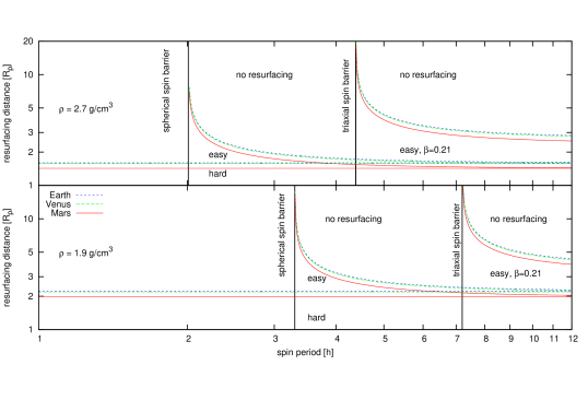
Figure 10: Best case ($r^{\star}_{easy}$) and worst case ($r^{\star}_{hard}$) resurfacing distances in planetary radii for an asteroid (see text for details) that has close encounters with Mars, Venus and the Earth. Resurfacing is possible for close encounter distances below the respective lines. Note that forces scale with asteroid diameter and this picture is therefore valid for any NEA size.

6.2.5 Dynamical simulations

We investigate the hypothesis of resurfacing by planetary encounters developed above by testing whether there is a significant difference in the number of potential resurfacing events between Q- and S-type asteroid samples. We probe the dynamical history of each asteroid by propagating its position together with a sample of 96 clones 0.5 Myrs into the past using a symplectic integrator based on Yoshida’s T+V split (Yoshida 1990) with General Relativity (GR) correction (Lubich et al. 2010). Symplectic integrators have the advantage that the error in the mean anomaly, i.e., the position on the planet on its orbit, does not grow as quickly as with standard propagators (Eggl and Dvorak 2010, and references therein). Using an 8^th order integrator with a stepsize of 1 day in the drift in mean anomaly over 0.5 Myrs is less than 0.015${}^{\textrm{o}}$ in the two-body problem Sun-Earth, corresponding to a total along track displacement of less than 6 Earth radii. As for close encounters, the propagator is able to resolve all close encounters lasting more than 6 hours reasonably well. The limit resolution is reached for encounters lasting three hours. While the integration algorithm is not regularized, care has been taken to avoid losing accuracy due to imprecise calculation of accelerations and the accumulation of round off errors (e.g., via the use of Kahan summation).
Each simulation contained the following massive perturbers: the 8 planets, the barycenter of the Pluto system as well the major asteroids (1) Ceres, (2) Pallas, (4) Vesta and (10) Hygiea, henceforth referred to as the massive bodies. Initial conditions for the massive bodies were taken from JPL DE405 ephemerides at the epoch J2000. The initial conditions for the asteroids were constructed using the open source software OrbFit  (Milani et al. 2008), taking all observations up to April 2014 into account. Asteroid orbits were fit to the non-relativistic dynamical system containing all planets and the Pluto system. No asteroid perturbers were taken into account during the fitting process. Given the timescales involved in the orbit fitting and differential correction, the discrepancies arising from neglecting GR and the major perturbing asteroids on the investigated asteroids can be considered small compared to the orbit uncertainties.
The uncertainty covariance matrix resulting from the orbital fit was then sampled along the line of variation (Milani et al. 2000) from -3$\sigma$ to +3$\sigma$ with 96 clones per asteroid. The 96 clones were then propagated together with the nominal orbit in order to see the dispersion in phase space. All close encounters, with the Earth, Venus, Mars, Jupiter and the main perturbing asteroids were cataloged for each clone in form of close minimum encounter distance (MED) and time histograms. The following limit distances were used to trigger a close encounter log: Jupiter: 2.56956 au, Venus, Earth and Mars: 0.256956 au, the main perturbing asteroids: 0.0256956 au. These values correspond to approximately 7 Hill’s radii for Jupiter, 25 for the Earth and Venus, 35 Hill’s radii for Mars and 35-70 Hill’s radii for the perturbing asteroids. Minimum encounter distances and velocities were calculated using cubic spline interpolation of the asteroid’s orbit during its close encounter. Global minimum and average encounter distances together with their variances were also saved. In addition, minimum orbit intersection distances (MOIDs) were calculated every 800 days. Similarly to the MED values, MOID histograms, averages and variances were cataloged.
It should be mentioned that results stemming from integrating NEO orbits backwards in time need to be interpreted with care. Similarly to forward propagation NEAs on chaotic trajectories with the terrestrial planets have a relatively short horizon that limits an accurate prediction of their dynamical evolution (see, e.g., Michel 1997) In such cases even robust ensemble statistics will not yield reliable estimates on close encounter distances since the divergence of nearby solution becomes exponential. As a consequence, we decided to exclude those NEAs from the statistics as soon as the spread in clone encounter distances becomes large. In our dynamical study, we also excluded the Yarkovsky effect for the following reasons. First, the spin state and orientation of the chosen targets are largely unknown. While this could be remedied using a statistical distribution of drift parameters among the clones of each NEA as proposed, for instance, by Spoto et al. (2014), this would only lead to an artificially increased spread in 96 clones making it harder to determine which NEAs are on chaotic orbits and which are not. Second, close encounters can change the spin state, making self-consistent predictions very difficult. That being said, Yarkovsky drift rates of our targets range between $10^{-4}$ and $10^{-3}$ au/Myr. The cross-track error that results from neglecting the Yarkovsky drift alone can range between 2–20 Earth radii over 0.5 Myrs, and along track position errors are much larger.
Regardless of the simplifications of our dynamical model, we find that all the Q-types have a minimum MOID allowing a close encounter with the Earth (18% of the sample), or Mars (100%) in the past 500,000 years (we use the median values from all the clones here). A large fraction of the S-type sample also present a minimum MOID that could have led to a close encounter with one of the terrestrial planets (12.9%, 6.7%, and 95.4% for the Earth, Venus, and Mars respectively), similarly to the situation presented by (Binzel et al. 2010) and (DeMeo et al. 2014b). However, a small MOID does not necessary imply a close encounter: the MOID provides a measure of the distance between the orbits, not between the bodies. The typical example would be a Trojan asteroid, for which the MOID is small by definition, but that would never encounter the planet.
To overcome this issue, we also study the minimum encounter distance (MED) of the asteroids and their clones: that is the real distance between the particles and the massive bodies. However, even with a symplectic integrator, the drift in mean anomaly steadily increases with ephemeris time, and reach the level of a few planetary radii, at which the resurfacing is deemed to occur (see 6.2.4 above). Results for MED therefore potentially suffer from an underestimation of the number of close encounters, especially for the closest. The total number of detected MED resurfacing events is much less than the theoretically favorable number of configurations given by the encounter numbers using MOIDs. However, MEDs share the same trends with our MOID results.
The analysis using the median properties of each asteroid with its 96 clones seems therefore not conclusive: based on MED values, the planetary encounters are not expected to play any role in rejuvenating the surface of the Q-types, and based on MOID values, there should be more fresh surfaces (i.e., less S-types) as the vast majority of our sample present small MOID with Mars. We therefore study the populations of S- and Q-types statistically. We present in Fig. 11 the cumulative number of close encounters reaching the planetary distance for easy and hard resurfacing scenarios (see 6.2.2 and 6.2.3) between our sample of asteroids and Venus, the Earth, and Mars. There is a clear difference in the number of encounters experienced by the population of Q-types compared to the S-types sample for both Venus and the Earth. That is, the asteroids presenting a fresh surface, similar to ordinary chondrites and exempt of signature from space weathering, tend to have more close encounters with massive bodies that those asteroids with space-weathered surface. Significant resurfacing would thus occur from the stress during repetitive close encounters with planets. The distribution of encounters for both the Earth and Venus clearly highlights the sample of Q-types among the NEAs sample presented here (and somewhat provides an a posteriori validation of our classification into S- and Q-types, the two groups being apparently dynamically different).
Conversely, the encounter distribution with Mars is similar for both taxonomic classes, as both could theoretically have numerous encounters with Mars, within the expected distance suitable for resurfacing to occur. Among all the parameters recorded during the dynamical simulation, none showed a significant difference between the two populations and we are therefore limited to speculations. Because the sample of MCs studied here exhibit larger diameters than the NEAs encountering the Earth, they are deemed to be older. Their surface may therefore have reached the saturation state introduced by Marchi et al. (2012), where rejunevation is inefficient. The frequent encounters with Mars would then no longer turn the S-type surfaces into Q-types. Another possibility is that the limit for easy resurfacing being tight to the rotation period and obliquity during the close encounter, only a small fraction of close encounters do trigger resurfacing events, with a preference for fast-spinning asteroids. A survey of rotation period of Q-types among NEAs and MCs population could address this point.

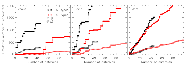
Figure 11: Comparison of the number of close encounters for the easy and hard resurfacing cases (filled and open symbols) for the samples of Q- and S-type asteroids (in black squares and red circles).

7 Conclusion

In this work, we report on the dynamical and surface properties of near-Earth asteroids (NEAs) and Mars-crosser asteroids (MCs), based on the analysis of their colors in the visible. Our sample includes:

• 43 NEAs and 310 MCs listed in the Moving Object Catalogue (MOC4) of the Sloan Digital Sky Survey (SDSS);

• 206 NEAs and 776 MCs, in publicly available images of the SDSS, using our citizen-science project “Near-Earth Asteroids Recovery Program” of the Spanish Virtual Observatory (SVO, Solano et al. 2013) measured in four filters (g^′, r^′, i^′, and z^′);

• 678 NEAs and MCs asteroids measured in three filters (g^′, r^′, and i^′) also from our citizen-science project, for 254 of which we assign tentative taxonomic classification.

In total we have determined the taxonomic class of these 982 NEAs and MCs using the DeMeo-Carry taxonomy for SDSS colors (DeMeo and Carry 2013), that is compatible with the Bus-DeMeo taxonomy based on V+NIR spectra (DeMeo et al. 2009)

The sample of taxonomic classes presented here correspond to an increase of known classes by 40% and 600% for NEA and MC populations, respectively. Among those, 36 NEAs can be considered potential targets for space missions, owing to their low $\delta v$. Some candidates for rare taxonomic classes such as D-, L-, and K-types are present within this sample and would benefit from further spectral investigations.
We then use the sample of asteroids with taxonomic classes based on four-filter observations to study their source regions and the effect of planetary encounters on their surface properties. To this end

• we compare the distribution of taxonomic classes between our sample of NEAs and MCs and the source regions, using the predictions resulting from the dynamical model presented by Greenstreet et al. (2012). The population of 2–5 km diameter asteroids in the main belt (DeMeo and Carry 2014) match closely the predictions from the sample presented here, supporting that the $\nu_{6}$ secular resonance and the 3:1 mean-motion resonance with Jupiter are the primary sources of kilometer-size NEAs;

• we analyze the dependence of spectral slope on diameter for asteroids in the S-complex. A linear trend of shallower slope toward higher absolute magnitude is found;

• we develop a simple force model on surface grains during a planetary encounter;

• we investigate the planetary distance at which a resurfacing event is expected to occur, by considering two extreme cases to the simple force model, when the conditions are the most or conversely the least conducive to favorable resurfacing event. This distance is found to be a function of the rotation period and density of the asteroid, and of the spin obliquity during the encounters. It ranges from 2 to $\approx$10 planetary radii for Venus, the Earth, and Mars. Such values are consistent with previous estimates by Binzel et al. (2010) and Nesvorný et al. (2010);

• we study the dynamical history of the sample of S- and Q-type by propagating their positions backward in time for 0.5 Myrs, together with 96 clones, using a symplectic post-Newtonian integrator. The population of Q-type presents statistically more encounters with Venus and the Earth at distance where resurfacing should occur than S-types. However, both populations present a high number of encounters with Mars and are indistinguishable.

Appendix A Forces model

In the following we will briefly discuss the force models used in equations (2) and (4).

A.1 Self gravity of the asteroid

On the surface of the asteroid a particle of mass $\mu$ will experience the following gravitational pull towards the asteroid’s center of mass:

$$F_{ga}=\mathcal{G}\mu m/R^{2}$$ (7)

where $\mathcal{G}$ is the gravitational constant, $m$ the mass and $R$ the local radius of the asteroid.

A.2 Forces due to the Rotating Frame

In a rotating frame of reference, surface particles are subject to a centrifugal force $F_{cf}$. It will suffice to consider principle axis rotation as we are primarily interested in best and worst case scenarios. Therefore, the particle feeling the maximum centrifugal acceleration then is located farthest from the axis of rotation and we have

$$F_{cf}=\mu R\omega^{2}\cos{\phi}$$ (8)

Here, $\omega$ is the spin rate and $\phi$ the angle between the asteroid’s spin axis and the vector $\vec{r}$ connecting the centers of gravity of the planet and the asteroid. In other words $\phi$ is the asteroid’s obliquity with respect to is planetocentric orbit. Consequently, $F_{cf}^{max}=\mu R^{max}\omega_{sb}^{2}$. This corresponds to a particle on the equator of a spherical asteroid with maximum radius $R^{max}$ and a rotation rate close to the spin barrier $\omega_{sb}$. As we assume that the particles are at rest on the surface, no Coriolis forces will have to be accounted for.

A.3 Tidal Acceleration

Asteroid that have close encounters with other massive bodies will experience tidal forces. Towards an asteroid’s surface the tidal acceleration becomes stronger compared to volume elements that are closer to the center of gravity. Consequently surface particles are pulled away more easily than say boulders close to the center of the asteroid. A simple model for the tidal force acting on a particle with mass $\mu$ is:

$$F_{td}=2R\mathcal{G}\mu M/D^{3}$$ (9)

where $M$ is the mass of the planet and $D$ the distance between the asteroid and the planet. In principle, there are additional tidal contributions from the sun, and the moon if the Earth is approached. Those are, however, small compared to the contribution of the Earth itself and shall, therefore, be neglected.

A.4 Particle Cohesion

The role of cohesion in rubble pile asteroids has been studied extensively over the past years (Scheeres et al. 2010; Hartzell and Scheeres 2011; Sánchez and Scheeres 2014). It is currently understood that particle cohesion plays and important role in determining limits for rubble-pile asteroid failures, fission, and for the survival of contact binaries. The standard cohesion model as presented in Hartzell and Scheeres (2011) is based on van der Waals interaction in granular materials. The inter particle force can be modeled as:

$$F_{co}=CS^{2}\sigma$$ (10)

where $C=5.14\times 10^{-2}\;kg/s^{2}$ is a material constant related to the Hamaker constant, $S\sim 1$ is the so-called cleanliness ratio, a qualitative factor indicating the impurity of granular surface coatings and $\sigma$ is the radius of the particles on the asteroid’s surface. For a detailed discussion of equation 10 see e.g. Hartzell and Scheeres (2011). As it is harder to free larger particles or rocks from the surface, we will increase the particle radius that shall be lifted against cohesion. Equation (10) illustrates that the larger the particles and the cleaner the surface, the larger the cohesive force. Let us now determine the approximate size of the largest particles that will be relevant for our resurfacing considerations. For this purpose we assume an $N\propto(2\sigma)^{-3}$ distribution of the number of particles $N$ on the asteroid’s surface. Using equation (36) in Sánchez and Scheeres (2014) we can calculate the particle diameter up to which smaller particles cover 99% of the surface. This is $\sigma=100r_{0}$, where we furthermore assume that $r_{0}$ is of the order of the smallest particle radii that could be detected on Itokawa ($r_{0}\simeq 10^{-6}$ m). Hence, practically all of the asteroid’s surface is covered by particles smaller than 0.1 millimeters.

Appendix B Taxonomic classifications

#	Name	Class	r′	$\delta$r′	i′	$\delta$i′	z′	$\delta$z′	a	e	i	H
									(au)	(${}^{\textrm{o}}$)
58070	1034 T-2	C	1.029	0.065	1.199	0.102	1.127	0.148	2.347	0.301	6.14	16.00
30717	1937 UD	S	1.282	0.067	1.424	0.048	1.192	0.058	2.168	0.334	8.96	14.00
118162	1951 SX	S	1.200	0.042	1.363	0.069	1.308	0.106	1.875	0.254	39.11	15.00
216464	1974 PB	V	1.237	0.038	1.416	0.056	1.104	0.071	2.318	0.341	6.57	17.00
136564	1977 VA	C	1.028	0.038	1.107	0.051	1.096	0.071	1.866	0.394	2.98	19.20
159368	1979 QB	S	1.207	0.023	1.272	0.002	1.085	0.031	2.330	0.443	3.35	17.00
120450	1982 SV	S	1.225	0.034	1.343	0.062	1.236	0.102	2.418	0.367	21.86	15.80
9292	1982 UE2	S	1.203	0.006	1.345	0.008	1.205	0.003	2.196	0.285	4.34	15.00
0	1983 QC	C	1.011	0.052	1.011	0.065	0.959	0.110	2.597	0.432	7.23	18.00
19958	1985 RN4	D	1.318	0.046	1.330	0.066	1.517	0.124	2.379	0.312	2.40	16.00
30771	1986 PO2	S	1.169	0.043	1.294	0.060	1.076	0.089	2.381	0.344	8.30	15.00
22283	1986 PY	D	1.266	0.041	1.381	0.058	1.539	0.114	2.189	0.247	7.98	14.00
15700	1987 QD	S	1.117	0.031	1.247	0.046	1.159	0.064	2.209	0.316	26.78	14.40
85158	1987 UT1	S	1.266	0.050	1.451	0.078	1.213	0.124	2.299	0.317	6.03	15.00
5510	1988 RF7	S	1.057	0.029	1.213	0.067	1.096	0.081	2.190	0.245	5.69	13.90
26822	1988 RG13	V	1.219	0.065	1.475	0.098	1.179	0.138	2.201	0.249	8.92	14.00
37568	1989 TP	X	1.106	0.050	1.202	0.070	1.215	0.125	1.796	0.100	22.76	15.00
6444	1989 WW	S	1.191	0.033	1.294	0.060	1.213	0.067	2.230	0.306	6.06	14.00
316651	1990 OL	S	1.214	0.017	1.372	0.012	1.248	0.017	2.690	0.455	14.83	15.00
16474	1990 QG3	U	1.260	0.039	1.395	0.063	2.054	0.162	2.237	0.301	1.65	16.00
65682	1990 QU2	S	1.196	0.076	1.354	0.054	1.234	0.051	2.212	0.247	7.60	15.00
160510	1990 RG1	S	1.229	0.050	1.487	0.082	1.433	0.124	2.263	0.267	6.58	15.00
5587	1990 SB	S	1.203	0.056	1.291	0.064	1.124	0.054	2.395	0.546	18.08	13.00
24693	1990 SB2	D	1.315	0.057	1.549	0.099	1.789	0.201	2.405	0.349	20.12	13.00
5645	1990 SP	X	1.108	0.037	1.211	0.065	1.281	0.121	1.355	0.387	13.51	17.00
30825	1990 TG1	S	1.191	0.041	1.254	0.022	1.118	0.026	2.437	0.681	8.74	14.70
5646	1990 TR	S	1.231	0.041	1.404	0.060	1.173	0.085	2.142	0.437	7.91	15.00
85185	1991 LM3	S	1.202	0.011	1.330	0.025	1.143	0.005	2.176	0.286	5.05	16.60
48468	1991 SS1	S	1.207	0.100	1.314	0.172	1.225	0.315	2.371	0.368	5.75	16.00
100045	1991 TK1	S	1.187	0.069	1.311	0.100	1.193	0.170	2.349	0.294	22.02	14.00
6454	1991 UG1	B	0.968	0.075	0.979	0.095	0.893	0.145	2.755	0.396	29.70	12.00
55757	1991 XN	C	1.053	0.052	1.091	0.067	1.042	0.132	2.320	0.288	8.59	15.00
21088	1992 BL2	L	1.200	0.050	1.327	0.071	1.379	0.125	1.707	0.238	38.46	14.00
32827	1992 DF1	S	1.210	0.022	1.347	0.018	1.192	0.042	2.281	0.311	21.19	15.00
6455	1992 HE	L	1.186	0.042	1.366	0.076	1.412	0.129	2.241	0.572	37.33	13.00
10115	1992 SK	S	1.193	0.060	1.337	0.045	1.180	0.017	1.248	0.325	15.32	17.00
0	1992 UB	X	1.100	0.047	1.122	0.063	1.148	0.139	3.085	0.577	15.94	16.00
79150	1992 UR7	S	1.097	0.040	1.395	0.070	1.177	0.102	2.178	0.271	7.91	16.00
26129	1993 DK	S	1.246	0.043	1.270	0.057	1.183	0.093	2.434	0.337	20.96	13.00
39572	1993 DQ1	S	1.163	0.028	1.336	0.015	1.129	0.019	2.036	0.493	10.03	16.00
5693	1993 EA	C	1.104	0.044	1.145	0.065	1.118	0.118	1.271	0.585	5.06	16.00
14461	1993 FL54	D	1.120	0.044	1.318	0.065	1.431	0.129	2.328	0.326	21.31	14.00
52384	1993 HZ5	C	1.009	0.028	1.086	0.050	1.225	0.068	1.852	0.102	26.23	15.70
145720	1993 OX7	S	1.191	0.044	1.368	0.063	1.180	0.098	2.583	0.359	6.85	16.10
7025	1993 QA	D	1.193	0.045	1.237	0.068	1.411	0.123	1.476	0.315	12.61	18.00
20062	1993 QB3	S	1.214	0.015	1.386	0.077	1.235	0.067	2.230	0.300	20.12	14.00
73735	1993 QE3	S	1.285	0.025	1.267	0.042	1.082	0.027	2.144	0.238	3.18	16.00
16635	1993 QO	X	1.085	0.010	1.096	0.010	1.115	0.020	2.299	0.284	21.94	13.90
16657	1993 UB	S	1.143	0.060	1.252	0.091	1.130	0.140	2.277	0.461	24.98	16.00
7660	1993 VM1	S	1.259	0.046	1.528	0.070	1.486	0.096	1.910	0.140	23.15	14.20
136617	1994 CC	S	1.195	0.058	1.232	0.083	1.022	0.115	1.638	0.417	4.68	17.00
136618	1994 CN2	S	1.203	0.045	1.277	0.066	1.204	0.135	1.573	0.395	1.44	16.00
79219	1994 LN	S	1.306	0.048	1.486	0.068	1.330	0.098	1.915	0.161	25.68	15.60
14017	1994 NS	S	1.222	0.026	1.334	0.013	1.298	0.012	2.167	0.240	6.48	14.00
52439	1994 QL	S	1.213	0.034	1.380	0.051	1.271	0.059	1.926	0.143	26.56	15.10
24814	1994 VW1	V	1.180	0.065	1.419	0.065	1.148	0.053	1.962	0.260	15.55	15.00
12390	1994 WB1	S	1.343	0.049	1.406	0.065	1.294	0.072	1.855	0.151	24.81	14.80
52453	1994 WC	C	1.028	0.007	1.057	0.001	1.068	0.004	2.420	0.330	11.46	14.00
160519	1995 CS3	K	1.159	0.032	1.247	0.046	1.180	0.065	2.274	0.336	1.94	16.00
100316	1995 MM2	S	1.261	0.016	1.278	0.043	1.089	0.024	2.211	0.251	4.85	16.00
48621	1995 OC	S	1.250	0.059	1.355	0.040	1.258	0.053	2.204	0.276	2.87	16.00
26166	1995 QN3	S	1.138	0.042	1.343	0.062	1.318	0.109	3.304	0.644	14.79	16.00
21228	1995 SC	C	0.996	0.034	1.039	0.046	0.962	0.082	2.762	0.398	28.32	15.00
55825	1995 SD4	S	1.196	0.038	1.405	0.060	1.327	0.101	2.153	0.226	3.93	15.00
368153	1995 UX1	S	1.170	0.058	1.331	0.089	1.252	0.160	2.658	0.443	15.18	17.00
162038	1996 DH	S	1.274	0.048	1.464	0.026	1.383	0.036	1.587	0.277	17.23	16.00
85372	1996 EO12	V	1.169	0.052	1.310	0.082	0.921	0.101	2.210	0.250	7.47	15.00
0	1996 ME	S	1.354	0.111	1.380	0.025	1.190	0.044	2.212	0.304	7.68	16.71
85383	1996 MS	D	1.152	0.032	1.263	0.049	1.570	0.106	2.589	0.363	6.88	15.00
23621	1996 PA	S	1.164	0.058	1.286	0.075	1.097	0.150	1.904	0.299	19.35	15.00
129541	1996 PQ9	S	1.179	0.048	1.354	0.074	1.257	0.114	2.274	0.302	19.61	14.00
21277	1996 TO5	V	1.189	0.044	1.267	0.060	0.976	0.080	2.379	0.519	20.95	16.00
39702	1996 TZ10	S	1.176	0.039	1.324	0.061	1.203	0.128	2.369	0.314	7.05	15.00
100493	1996 VK37	S	1.245	0.044	1.374	0.068	1.275	0.100	2.236	0.268	2.38	17.00
225312	1996 XB27	D	1.153	0.035	1.212	0.050	1.335	0.091	1.189	0.058	2.47	22.00
73865	1997 AW	C	0.987	0.035	1.061	0.047	1.092	0.075	2.378	0.368	1.73	15.00
100553	1997 GD	C	1.038	0.029	1.117	0.051	1.028	0.066	1.785	0.163	9.81	16.20
90916	1997 LR	S	1.194	0.043	1.379	0.067	1.319	0.117	2.200	0.285	7.38	16.00
9992	1997 TG19	X	1.064	0.037	1.210	0.057	1.208	0.103	2.170	0.293	2.60	14.00
14982	1997 TH19	S	1.228	0.037	1.357	0.047	1.241	0.076	2.329	0.322	3.32	14.00
35368	1997 UB8	S	1.235	0.001	1.374	0.009	1.216	0.004	2.332	0.313	22.72	14.00
16816	1997 UF9	S	1.194	0.048	1.276	0.069	1.184	0.110	1.442	0.604	25.91	16.00
27995	1997 WL2	S	1.221	0.025	1.346	0.026	1.247	0.019	2.124	0.272	3.46	14.00
160541	1997 WM58	C	0.994	0.047	1.024	0.057	0.982	0.103	2.268	0.270	7.90	15.00
28017	1997 YV13	X	1.068	0.063	1.155	0.075	1.178	0.171	2.599	0.387	4.98	13.00
31221	1998 BP26	S	1.249	0.020	1.413	0.011	1.343	0.015	1.723	0.257	20.22	17.00
31210	1998 BX7	S	1.159	0.054	1.275	0.079	1.056	0.116	2.606	0.502	8.96	16.00
136849	1998 CS1	S	1.253	0.034	1.326	0.050	1.232	0.081	1.491	0.578	7.79	17.00
19388	1998 DQ3	C	1.047	0.039	1.169	0.054	1.076	0.059	2.293	0.342	20.50	14.90
29566	1998 FK5	S	1.231	0.051	1.363	0.070	1.215	0.106	1.775	0.120	24.13	15.00
22601	1998 HD124	S	1.270	0.037	1.395	0.052	1.265	0.029	2.310	0.279	9.30	13.00
23726	1998 HG48	V	1.312	0.082	1.514	0.107	1.144	0.155	2.163	0.247	6.36	14.00
0	1998 HH145	S	1.271	0.047	1.247	0.057	1.086	0.080	2.200	0.244	5.13	16.94
136900	1998 HL49	V	1.187	0.072	1.290	0.103	0.914	0.129	1.743	0.636	11.02	17.00
12520	1998 HV78	S	1.181	0.052	1.290	0.077	1.180	0.127	2.247	0.294	4.80	14.00
136923	1998 JH2	D	1.307	0.044	1.350	0.063	1.487	0.121	2.133	0.442	6.62	16.00
44200	1998 MJ25	S	1.258	0.046	1.410	0.039	1.223	0.041	2.426	0.321	2.05	14.00
46818	1998 MZ24	S	1.111	0.057	1.293	0.088	1.154	0.149	2.336	0.331	21.52	13.00
25037	1998 QC37	C	1.067	0.039	1.138	0.042	1.096	0.061	2.198	0.256	4.79	15.00
190327	1998 QE85	C	0.969	0.028	1.142	0.047	1.154	0.072	2.207	0.249	7.11	16.00
373416	1998 QG1	C	1.073	0.034	1.167	0.049	1.151	0.084	2.376	0.443	6.41	17.00
101027	1998 QL71	S	1.270	0.047	1.368	0.013	1.224	0.034	2.295	0.291	7.01	15.40
28085	1998 QO98	S	1.211	0.002	1.347	0.002	1.268	0.000	2.262	0.314	19.86	14.00
79611	1998 RC52	S	1.213	0.019	1.391	0.016	1.261	0.065	2.349	0.299	5.82	15.00
58980	1998 RG47	S	1.222	0.060	1.368	0.084	1.303	0.169	2.212	0.267	5.49	15.00
66063	1998 RO1	S	1.099	0.003	1.179	0.003	1.099	0.004	0.991	0.720	22.68	18.00
0	1998 RZ13	Q	1.159	0.000	1.247	0.057	1.053	0.024	2.293	0.274	4.23	18.02
101258	1998 SF97	S	1.355	0.037	1.514	0.056	1.271	0.070	2.310	0.283	3.69	16.10
85709	1998 SG36	S	1.198	0.008	1.383	0.060	1.267	0.076	1.646	0.338	24.84	15.00
0	1998 SP49	S	1.232	0.027	1.266	0.027	1.089	0.058	2.320	0.335	4.97	16.86
96562	1998 SZ138	S	1.235	0.031	1.384	0.025	1.178	0.031	2.118	0.303	5.00	15.00
27089	1998 UE15	S	1.228	0.069	1.430	0.066	1.313	0.073	2.168	0.236	8.87	15.00
237416	1998 UT19	C	0.991	0.036	1.047	0.048	0.964	0.062	2.558	0.349	13.43	16.00
0	1998 UX24	X	1.059	0.014	1.089	0.023	1.158	0.001	1.836	0.286	14.12	20.00
101430	1998 VE32	S	1.201	0.071	1.383	0.099	1.171	0.148	1.857	0.290	26.98	15.00
31367	1998 WB9	S	1.228	0.035	1.417	0.016	1.241	0.036	2.330	0.317	24.23	13.00
0	1998 WC2	V	1.177	0.051	1.309	0.080	1.020	0.085	2.552	0.562	26.60	18.00
137069	1998 WQ15	S	1.235	0.002	1.340	0.046	1.140	0.044	2.536	0.355	9.51	16.00
22753	1998 WT	Q	1.083	0.051	1.172	0.072	0.923	0.089	1.219	0.570	3.21	17.00
0	1998 WT7	U	1.953	0.081	2.119	0.119	1.213	0.102	1.152	0.110	40.70	18.00
326306	1998 XY4	Q	1.073	0.014	1.208	0.001	1.008	0.024	2.607	0.375	30.22	16.00
85848	1998 YP29	S	1.248	0.017	1.393	0.022	1.275	0.046	2.199	0.278	6.87	17.00
129737	1999 AA9	B	0.978	0.012	0.980	0.017	0.921	0.028	2.096	0.266	4.44	16.00
31415	1999 AK23	V	1.301	0.027	1.372	0.033	0.872	0.039	2.274	0.270	6.85	14.00
101554	1999 AL4	S	1.243	0.029	1.322	0.029	1.138	0.015	2.346	0.334	21.85	15.40
121007	1999 AT9	V	1.181	0.091	1.282	0.115	0.865	0.150	2.277	0.330	11.01	15.00
231716	1999 BT2	S	1.180	0.033	1.330	0.049	1.202	0.066	2.407	0.340	23.82	15.00
257581	1999 FE8	C	1.098	0.010	1.060	0.058	1.039	0.043	2.558	0.377	27.00	16.00
38063	1999 FH	L	1.287	0.096	1.525	0.109	1.607	0.298	2.341	0.294	11.88	14.00
0	1999 FN19	S	1.152	0.027	1.245	0.070	1.110	0.068	1.646	0.391	2.30	22.00
101742	1999 FO7	C	1.076	0.040	1.067	0.039	1.057	0.058	2.386	0.343	23.23	14.70
40263	1999 FQ5	S	1.236	0.042	1.419	0.064	1.341	0.117	1.495	0.161	25.84	17.00
0	1999 FU81	S	1.148	0.042	1.368	0.063	1.159	0.096	2.353	0.298	5.15	17.97
66251	1999 GJ2	A	1.321	0.062	1.610	0.107	1.474	0.221	1.536	0.198	11.28	16.00
306459	1999 GS3	S	1.128	0.021	1.263	0.029	1.081	0.020	2.613	0.425	28.13	16.00
368160	1999 HW2	V	1.245	0.039	1.458	0.068	1.171	0.093	2.613	0.405	27.13	16.00
20446	1999 JB80	K	1.180	0.043	1.202	0.055	1.191	0.088	2.303	0.336	22.57	14.00
85989	1999 JD6	X	1.047	0.037	1.133	0.053	1.161	0.116	0.883	0.633	17.06	17.00
38181	1999 JG124	S	1.190	0.018	1.343	0.043	1.213	0.008	2.310	0.288	23.90	14.00
53319	1999 JM8	C	1.037	0.039	1.135	0.004	1.127	0.006	2.711	0.649	13.83	15.00
101811	1999 JQ6	S	1.216	0.022	1.263	0.046	1.101	0.046	2.363	0.321	22.22	14.70
40271	1999 JT	S	1.318	0.046	1.496	0.075	1.454	0.115	2.294	0.274	23.87	14.00
38091	1999 JT3	C	1.083	0.034	1.135	0.048	1.098	0.072	2.172	0.400	9.35	16.00
243618	1999 JU61	L	1.240	0.049	1.393	0.076	1.392	0.129	2.435	0.361	7.78	16.00
66358	1999 JW87	K	1.144	0.007	1.275	0.021	1.262	0.022	2.315	0.315	7.47	15.00
137173	1999 JY4	C	1.038	0.038	1.067	0.049	0.895	0.066	2.200	0.245	8.93	16.70
0	1999 KQ6	C	0.985	0.034	1.046	0.051	0.992	0.081	2.666	0.407	10.83	16.00
312979	1999 KT4	X	1.154	0.047	1.147	0.059	1.156	0.112	2.212	0.368	2.29	17.00
40310	1999 KU4	C	1.006	0.025	1.031	0.025	1.043	0.108	2.196	0.404	8.44	16.00
137199	1999 KX4	V	1.287	0.043	1.397	0.060	0.965	0.062	1.457	0.293	16.57	16.00
74561	1999 LE18	S	1.168	0.033	1.261	0.045	1.111	0.058	2.203	0.259	7.68	15.00
173245	1999 LY7	S	1.270	0.049	1.368	0.069	1.230	0.111	2.269	0.275	6.16	16.00
86039	1999 NC43	S	1.173	0.055	1.254	0.083	1.050	0.111	1.759	0.579	7.12	15.00
222079	1999 NE43	V	1.245	0.043	1.389	0.067	0.966	0.083	2.193	0.354	10.36	17.00
129813	1999 NJ	U	1.445	0.056	1.678	0.090	1.306	0.137	2.339	0.295	6.41	16.00
66419	1999 NR13	S	1.177	0.030	1.352	0.049	1.281	0.075	2.367	0.339	20.22	14.00
23983	1999 NS11	S	1.203	0.086	1.424	0.106	1.258	0.109	2.300	0.308	7.08	15.00
96744	1999 OW3	V	1.142	0.056	1.209	0.068	0.791	0.085	2.092	0.780	34.95	14.00
121210	1999 QG2	S	1.259	0.046	1.472	0.068	1.432	0.119	2.384	0.334	8.39	16.10
152771	1999 RB34	S	1.197	0.004	1.311	0.033	1.133	0.077	2.626	0.388	27.70	15.00
0	1999 RC31	L	1.185	0.040	1.308	0.060	1.331	0.103	2.579	0.467	26.26	16.00
192642	1999 RD32	C	1.019	0.000	1.028	0.012	1.054	0.022	2.642	0.770	6.79	16.00
368163	1999 RE198	U	0.374	0.011	4.976	0.307	6.787	0.878	2.235	0.300	8.31	17.00
0	1999 RF14	S	1.225	0.034	1.306	0.048	1.169	0.065	2.296	0.282	20.82	14.28
137230	1999 RG22	S	1.230	0.028	1.312	0.042	1.179	0.065	2.339	0.298	22.39	15.60
22807	1999 RK7	L	1.272	0.041	1.494	0.072	1.516	0.109	2.174	0.244	2.07	15.00
59836	1999 RN44	S	1.155	0.012	1.283	0.021	1.107	0.049	2.330	0.291	12.63	15.00
44619	1999 RO42	S	1.306	0.036	1.406	0.065	1.247	0.069	2.134	0.228	5.49	16.20
181898	1999 RS168	S	1.196	0.053	1.324	0.071	1.258	0.126	2.266	0.266	6.41	16.00
22844	1999 RU111	C	1.040	0.042	1.044	0.052	0.984	0.082	2.885	0.434	28.39	13.00
42887	1999 RV155	S	1.225	0.034	1.306	0.060	1.236	0.068	2.141	0.242	2.86	15.40
333901	1999 RX112	S	1.112	0.044	1.302	0.073	1.219	0.122	2.680	0.388	7.79	16.00
101952	1999 RY31	L	1.318	0.049	1.380	0.064	1.432	0.106	2.253	0.317	7.94	16.10
217686	1999 RY90	S	1.259	0.002	1.493	0.026	1.330	0.125	2.230	0.276	6.52	16.00
306479	1999 SE16	V	1.213	0.062	1.366	0.082	1.091	0.151	2.520	0.350	14.94	16.00
0	1999 SO15	V	1.339	0.012	1.441	0.028	1.009	0.027	2.232	0.296	8.55	17.00
121324	1999 SQ5	C	1.047	0.048	1.127	0.062	1.000	0.083	1.941	0.174	23.53	16.10
13819	1999 SX5	S	1.259	0.035	1.318	0.049	1.169	0.075	2.318	0.304	23.47	13.20
74789	1999 SY5	S	1.230	0.005	1.334	0.016	1.192	0.001	2.328	0.321	23.22	14.00
279776	1999 TA122	K	1.152	0.001	1.252	0.014	1.195	0.009	2.114	0.277	1.64	17.00
86212	1999 TG21	S	1.215	0.098	1.372	0.137	1.216	0.248	2.316	0.310	25.38	14.00
25362	1999 TH24	S	1.145	0.049	1.372	0.016	1.248	0.052	2.286	0.311	20.51	14.00
0	1999 TK271	V	1.180	0.030	1.303	0.047	0.728	0.036	2.260	0.313	4.80	17.00
162215	1999 TL12	Q	1.141	0.049	1.149	0.065	0.959	0.081	1.081	0.436	17.34	18.00
216947	1999 TM258	S	1.259	0.032	1.336	0.047	1.160	0.061	2.248	0.266	2.60	17.00
0	1999 TN169	C	1.057	0.039	1.028	0.047	1.000	0.074	2.328	0.289	5.54	17.10
36183	1999 TX16	L	1.315	0.056	1.417	0.079	1.442	0.151	1.551	0.333	38.22	16.00
0	1999 UH56	S	1.247	0.034	1.271	0.070	1.225	0.102	2.417	0.311	1.65	17.64
102528	1999 US3	L	1.143	0.126	1.261	0.125	1.285	0.369	2.751	0.524	29.11	13.00
102803	1999 VA169	S	1.251	0.033	1.326	0.040	1.100	0.067	2.135	0.236	4.85	16.60
43017	1999 VA2	S	1.213	0.045	1.368	0.063	1.282	0.083	2.271	0.289	23.91	15.50
162273	1999 VL12	K	1.159	0.051	1.290	0.075	1.279	0.139	1.594	0.236	20.19	17.00
75079	1999 VN24	S	1.250	0.040	1.431	0.062	1.262	0.092	2.316	0.294	23.00	13.00
0	1999 VS6	U	2.342	0.082	2.539	0.120	2.094	0.166	1.198	0.223	27.97	19.00
20691	1999 VY72	S	1.294	0.036	1.393	0.064	1.282	0.071	2.365	0.310	22.23	13.20
329282	1999 WZ5	U	1.960	0.053	1.312	0.047	3.230	0.215	2.310	0.342	27.53	16.00
45074	1999 XA38	U	1.794	0.100	1.954	0.144	1.364	0.191	2.212	0.252	5.22	15.00
102997	1999 XF94	S	1.257	0.045	1.451	0.067	1.226	0.099	2.279	0.299	22.96	14.00
333948	1999 XG135	C	0.993	0.003	1.075	0.003	1.104	0.068	2.959	0.504	11.39	16.00
80356	1999 XM124	V	1.368	0.038	1.629	0.060	1.330	0.074	2.181	0.246	4.69	16.10
0	1999 XM136	S	1.225	0.034	1.368	0.050	1.236	0.068	2.625	0.423	26.46	15.29
310429	1999 XP19	S	1.210	0.016	1.311	0.006	1.262	0.027	2.458	0.428	5.67	15.00
102910	1999 XT19	K	1.186	0.080	1.279	0.110	1.208	0.219	2.261	0.283	5.02	15.00
306522	1999 XZ14	K	1.138	0.047	1.307	0.077	1.253	0.150	2.320	0.326	23.75	15.00
249685	1999 YD4	S	1.211	0.065	1.345	0.031	1.186	0.082	2.364	0.299	23.32	15.00
145962	1999 YH5	S	1.100	0.060	1.261	0.087	1.113	0.133	2.254	0.325	24.85	15.00
45251	1999 YN	S	1.191	0.033	1.343	0.062	1.191	0.077	2.335	0.318	22.88	13.90
137802	1999 YT	S	1.175	0.039	1.408	0.070	1.164	0.095	1.776	0.352	31.58	17.00
50143	2000 AB132	S	1.189	0.041	1.327	0.061	1.177	0.104	2.274	0.280	6.62	15.00
86401	2000 AF143	S	1.206	0.061	1.348	0.095	1.084	0.170	2.335	0.292	5.40	14.00
310434	2000 AP146	L	1.173	0.038	1.356	0.061	1.415	0.099	2.547	0.417	23.51	15.00
31832	2000 AP59	S	1.266	0.053	1.396	0.032	1.301	0.039	2.183	0.265	6.59	14.00
26471	2000 AS152	S	1.169	0.032	1.282	0.047	1.107	0.061	1.918	0.154	19.69	13.00
103501	2000 AT245	S	1.213	0.025	1.325	0.042	1.158	0.046	2.276	0.287	22.51	14.80
103506	2000 BD1	C	1.030	0.059	1.076	0.081	1.069	0.187	1.969	0.267	27.10	15.00
219275	2000 BL11	L	1.204	0.038	1.296	0.054	1.366	0.096	2.289	0.279	5.64	17.00
0	2000 CB130	C	1.044	0.042	0.936	0.053	1.111	0.116	2.133	0.314	0.89	18.00
75933	2000 CB75	C	0.997	0.029	1.084	0.033	1.097	0.028	2.554	0.368	33.42	14.00
0	2000 CD32	V	1.196	0.034	1.363	0.051	1.092	0.065	1.791	0.233	24.47	17.00
138013	2000 CN101	S	1.204	0.011	1.335	0.024	1.231	0.077	1.599	0.635	15.95	14.00
103732	2000 CO103	S	1.180	0.033	1.294	0.048	1.236	0.091	2.260	0.284	22.46	14.80
31843	2000 CQ80	S	1.207	0.018	1.353	0.015	1.141	0.034	2.204	0.293	20.34	14.00
36282	2000 CT98	S	1.191	0.044	1.355	0.062	1.159	0.085	2.233	0.261	6.91	14.80
27346	2000 DN8	S	1.209	0.067	1.347	0.109	1.285	0.191	1.875	0.399	36.94	15.00
27351	2000 DO73	S	1.294	0.001	1.458	0.021	1.256	0.037	2.288	0.276	3.61	14.00
152931	2000 EA107	S	1.166	0.053	1.229	0.076	1.069	0.114	0.930	0.456	28.58	15.00
31869	2000 EF101	S	1.259	0.047	1.444	0.036	1.384	0.026	2.270	0.270	7.00	14.00
301964	2000 EJ37	D	1.122	0.020	1.289	0.034	1.397	0.019	4.635	0.706	10.05	13.00
86608	2000 EK85	S	1.231	0.046	1.407	0.074	1.252	0.135	2.264	0.280	8.59	15.00
0	2000 EN172	C	1.107	0.041	1.148	0.053	1.028	0.076	2.624	0.373	28.01	15.87
28565	2000 EO58	S	1.402	0.074	1.402	0.031	1.221	0.041	2.178	0.285	5.33	14.00
138131	2000 ES20	S	1.282	0.047	1.380	0.076	1.159	0.096	2.453	0.339	22.72	16.40
301962	2000 ET26	S	1.171	0.043	1.379	0.070	1.115	0.090	2.610	0.435	26.46	15.00
185854	2000 EU106	K	1.125	0.069	1.344	0.121	1.284	0.271	2.351	0.373	21.32	15.00
0	2000 EU70	C	1.088	0.041	1.106	0.057	1.034	0.120	2.211	0.763	13.00	18.00
86626	2000 EV124	S	1.191	0.065	1.297	0.047	1.127	0.003	2.161	0.266	7.35	15.00
33836	2000 FB39	S	1.193	0.132	1.315	0.188	1.216	0.270	2.377	0.343	14.62	15.00
219319	2000 FH10	S	1.255	0.094	1.330	0.140	1.271	0.273	1.655	0.114	9.84	18.00
162433	2000 FK10	C	1.026	0.044	1.159	0.065	1.056	0.099	1.359	0.482	13.94	19.00
31881	2000 FL15	S	1.121	0.050	1.243	0.075	1.154	0.128	1.784	0.114	21.08	16.00
86667	2000 FO10	S	1.257	0.068	1.289	0.107	1.079	0.171	0.859	0.595	14.28	17.00
30105	2000 FO3	S	1.221	0.004	1.377	0.012	1.316	0.020	2.176	0.312	7.32	14.00
118569	2000 GF1	S	1.152	0.035	1.299	0.007	1.134	0.015	2.310	0.293	23.83	15.00
269881	2000 GF15	S	1.278	0.050	1.444	0.000	1.316	0.147	2.398	0.311	5.35	16.00
60735	2000 GF82	K	1.225	0.045	1.259	0.058	1.213	0.078	2.345	0.330	21.74	14.90
51075	2000 GG162	S	1.395	0.039	1.310	0.049	1.215	0.077	2.333	0.317	21.83	14.00
97679	2000 GG2	S	1.212	0.041	1.322	0.061	1.194	0.092	1.571	0.132	50.81	16.00
152978	2000 GJ147	X	1.105	0.036	1.244	0.053	1.316	0.098	1.162	0.237	25.01	19.00
50867	2000 GM4	S	1.254	0.022	1.324	0.045	1.198	0.034	2.285	0.280	22.35	15.40
152964	2000 GP82	S	1.202	0.044	1.432	0.066	1.355	0.087	1.396	0.393	13.23	17.00
51157	2000 HB57	S	1.310	0.016	1.434	0.049	1.254	0.027	2.255	0.306	3.93	16.00
122106	2000 HC86	S	1.209	0.069	1.348	0.102	1.217	0.167	2.411	0.316	7.59	16.00
168710	2000 HE41	S	1.225	0.056	1.294	0.072	1.202	0.089	2.151	0.249	9.43	16.30
0	2000 HV80	S	1.241	0.029	1.324	0.006	1.126	0.052	2.377	0.412	6.99	17.43
41440	2000 HZ23	S	1.309	0.051	1.589	0.087	1.463	0.152	1.576	0.211	15.11	19.00
33881	2000 JK66	V	1.250	0.004	1.390	0.004	0.947	0.028	2.213	0.291	11.17	14.00
344143	2000 JQ3	C	1.100	0.000	1.095	0.065	0.948	0.000	2.464	0.488	7.81	18.00
0	2000 JT3	S	1.213	0.045	1.330	0.049	1.213	0.089	2.348	0.323	14.72	16.00
0	2000 KL33	Q	1.076	0.036	1.262	0.061	1.027	0.081	2.114	0.430	6.91	19.00
237486	2000 KM2	L	1.090	0.042	1.318	0.069	1.331	0.109	2.253	0.301	25.66	16.00
32122	2000 LD10	S	1.232	0.058	1.416	0.080	1.348	0.164	2.364	0.333	14.27	14.00
160085	2000 LJ6	S	1.276	0.039	1.471	0.065	1.256	0.085	2.260	0.296	22.70	15.00
45764	2000 LV	V	1.134	0.001	1.216	0.005	0.923	0.031	2.417	0.317	6.71	14.00
18109	2000 NG11	X	1.058	0.033	1.058	0.047	1.147	0.088	1.881	0.368	0.81	17.00
165139	2000 NJ10	Q	1.143	0.084	1.214	0.117	1.017	0.168	2.249	0.308	2.73	16.00
0	2000 OA22	L	1.165	0.045	1.282	0.064	1.362	0.101	2.724	0.483	10.12	17.00
18919	2000 OJ52	S	1.215	0.076	1.377	0.122	1.247	0.239	2.576	0.434	7.22	15.00
34048	2000 OR35	C	1.056	0.036	1.183	0.060	1.075	0.097	2.211	0.260	7.86	15.00
171671	2000 PF32	S	1.210	0.050	1.403	0.079	1.148	0.111	2.252	0.311	7.02	17.00
363076	2000 PH6	C	1.004	0.059	1.039	0.075	1.036	0.154	2.695	0.513	10.50	17.00
67399	2000 PJ6	B	0.915	0.029	1.052	0.042	0.993	0.067	1.301	0.346	14.69	18.00
160092	2000 PL6	S	1.172	0.016	1.277	0.006	1.122	0.005	2.378	0.356	21.72	14.50
159463	2000 PM7	C	0.980	0.009	1.061	0.042	1.048	0.043	2.371	0.339	7.95	16.00
134863	2000 PX5	L	1.219	0.050	1.231	0.068	1.247	0.120	2.100	0.359	4.56	17.00
0	2000 PZ5	C	1.072	0.009	1.169	0.001	1.054	0.005	2.825	0.520	3.65	17.00
0	2000 QB56	C	1.086	0.040	1.127	0.052	1.057	0.078	2.266	0.332	9.04	17.83
18181	2000 QD34	S	1.336	0.056	1.431	0.079	1.345	0.125	2.339	0.296	21.19	13.00
0	2000 QE203	S	1.281	0.030	1.417	0.031	1.360	0.044	2.167	0.312	6.06	18.00
237495	2000 QF56	V	1.122	0.054	1.230	0.098	0.941	0.157	2.299	0.276	10.52	16.00
87311	2000 QJ1	S	1.150	0.033	1.278	0.051	1.112	0.078	1.590	0.512	7.69	16.00
97886	2000 QK54	B	0.971	0.057	0.976	0.067	0.954	0.117	2.312	0.322	6.07	16.00
122358	2000 QM49	S	1.192	0.090	1.326	0.122	1.230	0.248	2.312	0.324	1.42	16.00
247062	2000 QN115	U	1.882	0.031	3.113	0.019	3.270	0.007	2.250	0.267	1.88	17.00
162551	2000 QS226	S	1.067	0.039	1.236	0.057	1.076	0.079	2.275	0.320	23.07	16.00
239881	2000 QW55	S	1.255	0.075	1.406	0.101	1.284	0.156	2.323	0.284	5.49	16.00
24447	2000 QY1	S	1.206	0.038	1.399	0.058	1.220	0.080	1.724	0.235	12.25	17.00
350535	2000 QY44	D	1.375	0.052	1.482	0.072	1.594	0.126	2.428	0.333	3.52	17.00
122421	2000 QZ101	S	1.148	0.032	1.282	0.059	1.107	0.071	2.210	0.260	6.48	15.80
285631	2000 RB84	C	1.054	0.014	1.044	0.003	0.976	0.006	2.351	0.293	5.89	16.00
67502	2000 RE44	C	1.009	0.037	1.038	0.057	0.955	0.070	2.324	0.330	5.14	15.00
0	2000 RF43	S	1.117	0.031	1.213	0.045	1.138	0.073	3.006	0.455	9.96	15.18
162566	2000 RJ34	C	1.013	0.007	0.984	0.039	0.974	0.001	2.634	0.575	13.86	15.00
189552	2000 RL77	Q	1.134	0.057	1.243	0.093	1.050	0.135	2.555	0.536	30.30	16.00
329301	2000 RM77	S	1.348	0.042	1.246	0.050	1.196	0.082	2.627	0.376	29.61	15.00
190543	2000 RM80	S	1.185	0.043	1.281	0.063	1.089	0.093	2.546	0.359	6.18	17.00
162567	2000 RW37	C	1.102	0.034	1.096	0.044	0.930	0.067	1.248	0.250	13.75	20.00
234242	2000 SC340	S	1.147	0.059	1.186	0.079	1.027	0.140	2.298	0.329	5.63	16.00
0	2000 SD372	U	0.846	0.028	0.887	0.043	0.900	0.078	2.337	0.294	8.30	17.00
159477	2000 SE	S	1.271	0.036	1.278	0.048	1.235	0.073	2.384	0.363	6.54	16.00
20790	2000 SE45	S	1.120	0.054	1.220	0.076	1.067	0.131	2.739	0.562	8.34	16.00
0	2000 SF137	S	1.189	0.023	1.383	0.003	1.259	0.060	2.572	0.372	6.10	17.00
0	2000 SF8	S	1.236	0.045	1.333	0.064	1.145	0.099	1.649	0.345	17.44	20.00
93040	2000 SG	S	1.158	0.043	1.336	0.018	1.180	0.011	2.442	0.375	20.43	13.50
0	2000 SH52	X	1.114	0.046	1.234	0.068	1.275	0.128	2.244	0.264	2.63	18.00
0	2000 SL	S	1.195	0.063	1.318	0.095	1.175	0.177	1.540	0.395	38.35	18.00
0	2000 SL10	Q	1.157	0.044	1.208	0.066	1.020	0.102	1.372	0.339	1.46	21.00
76828	2000 SL161	A	1.389	0.038	1.580	0.061	1.355	0.077	1.998	0.222	11.70	16.00
0	2000 SL55	V	1.143	0.055	1.367	0.080	1.100	0.120	2.296	0.290	2.15	18.00
203117	2000 SN218	S	1.184	0.028	1.310	0.011	1.141	0.021	2.361	0.321	7.29	16.00
373469	2000 SO42	C	1.004	0.045	1.053	0.066	1.051	0.118	2.648	0.439	10.80	16.00
105674	2000 SQ42	X	1.169	0.057	1.112	0.070	1.122	0.130	2.301	0.340	22.31	15.00
326350	2000 SS217	V	1.224	0.016	1.322	0.014	1.049	0.019	2.154	0.295	7.01	17.00
36779	2000 SW1	V	1.199	0.031	1.273	0.047	0.979	0.054	2.303	0.308	7.65	15.00
189054	2000 SW278	C	1.094	0.081	1.117	0.098	1.026	0.256	2.578	0.364	17.09	15.00
0	2000 SX162	X	1.133	0.053	1.188	0.083	1.192	0.150	2.374	0.450	6.33	17.00
105943	2000 SY233	K	1.107	0.071	1.294	0.083	1.282	0.071	2.278	0.303	5.42	16.90
252050	2000 SZ10	C	1.027	0.044	1.064	0.070	1.057	0.120	2.243	0.287	22.71	17.00
368188	2000 SZ72	U	1.238	0.000	1.204	0.045	5.388	0.436	2.189	0.269	4.89	17.00
313085	2000 TB45	S	1.223	0.032	1.321	0.004	1.225	0.016	2.305	0.278	5.34	17.00
0	2000 TL1	C	1.002	0.039	0.964	0.048	0.966	0.083	1.338	0.300	3.61	22.00
162694	2000 UH11	U	1.099	0.035	1.873	0.091	6.469	0.641	0.870	0.422	32.23	19.00
67729	2000 UQ23	S	1.170	0.006	1.416	0.005	1.284	0.006	2.191	0.249	3.67	16.00
333305	2000 VB35	L	1.163	0.053	1.341	0.082	1.391	0.166	2.587	0.366	7.61	16.00
138847	2000 VE62	S	1.224	0.080	1.310	0.111	1.128	0.165	1.619	0.287	22.18	16.00
334012	2000 VF12	D	1.115	0.040	1.282	0.064	1.431	0.170	2.584	0.370	6.17	16.00
138846	2000 VJ61	C	1.011	0.058	1.136	0.090	0.958	0.145	2.185	0.563	18.67	15.00
331548	2000 VO47	S	1.204	0.034	1.378	0.054	1.352	0.089	2.624	0.379	27.33	15.00
71997	2000 WD178	S	1.192	0.040	1.352	0.049	1.163	0.112	2.293	0.299	7.24	15.00
162741	2000 WG6	U	0.912	0.027	0.973	0.041	2.708	0.232	2.320	0.497	11.82	17.00
106589	2000 WN107	C	1.098	0.017	1.104	0.018	1.061	0.040	2.150	0.614	14.33	16.00
165394	2000 XC15	S	1.169	0.032	1.282	0.059	1.107	0.061	2.335	0.295	22.21	14.90
217807	2000 XK44	L	1.203	0.037	1.326	0.054	1.346	0.105	1.724	0.385	11.24	18.00
0	2000 YG4	Q	1.090	0.038	1.169	0.053	1.015	0.076	2.211	0.503	2.57	20.00
39235	2000 YH55	V	1.028	0.033	1.256	0.056	0.947	0.076	2.353	0.311	14.17	14.00
344161	2000 YK18	C	1.021	0.019	1.083	0.007	1.059	0.011	2.515	0.342	6.64	16.00
63160	2000 YN8	S	1.193	0.040	1.361	0.065	1.192	0.102	2.186	0.254	7.77	15.00
63164	2000 YU14	S	1.301	0.039	1.390	0.058	1.330	0.088	2.272	0.306	3.33	15.00
316934	2001 AA52	S	1.250	0.044	1.333	0.061	1.093	0.080	2.323	0.287	9.13	16.00
0	2001 AT47	S	1.186	0.011	1.231	0.060	1.095	0.083	2.659	0.482	25.81	15.00
138925	2001 AU43	X	1.050	0.044	1.164	0.066	1.199	0.119	1.897	0.377	72.15	15.00
165494	2001 BD42	S	1.242	0.006	1.360	0.056	1.209	0.100	2.395	0.306	22.76	15.90
310535	2001 BJ43	S	1.182	0.055	1.265	0.073	1.071	0.093	1.966	0.232	9.75	17.00
94210	2001 BK33	S	1.208	0.006	1.361	0.006	1.199	0.033	2.557	0.381	5.16	15.20
98891	2001 BK41	C	1.057	0.029	1.117	0.051	1.076	0.079	2.322	0.389	7.59	15.90
160137	2001 BU41	Q	1.086	0.030	1.180	0.043	1.000	0.064	2.396	0.328	20.50	15.10
171784	2001 BV67	S	1.202	0.044	1.306	0.048	1.138	0.063	2.337	0.340	7.35	16.80
107150	2001 BW10	V	1.256	0.040	1.482	0.068	1.093	0.074	2.187	0.319	20.26	15.00
76978	2001 BY60	S	1.229	0.059	1.426	0.093	1.235	0.154	2.225	0.319	26.87	14.00
0	2001 CQ36	U	1.579	0.065	1.303	0.068	1.091	0.102	0.938	0.177	1.26	22.00
0	2001 DS8	U	0.837	0.036	0.938	0.063	0.912	0.103	2.126	0.515	2.42	22.00
337328	2001 DU40	S	1.170	0.018	1.245	0.028	1.047	0.043	2.559	0.375	9.69	16.00
72569	2001 EC13	S	1.178	0.029	1.332	0.053	1.171	0.061	2.349	0.295	24.75	14.00
347584	2001 EH18	S	1.173	0.055	1.332	0.084	1.196	0.000	2.553	0.363	34.03	15.00
26677	2001 EJ18	S	1.296	0.063	1.488	0.095	1.348	0.146	1.540	0.019	27.75	16.00
228404	2001 EQ17	V	1.214	0.051	1.306	0.078	1.006	0.088	2.183	0.246	24.72	16.00
0	2001 FA97	C	1.009	0.028	0.982	0.045	0.982	0.054	2.758	0.413	11.05	15.92
68278	2001 FC7	C	1.062	0.017	1.055	0.010	1.022	0.009	1.436	0.115	2.62	18.00
63341	2001 FD77	S	1.234	0.003	1.338	0.007	1.175	0.010	2.626	0.387	27.97	13.00
249816	2001 FD90	V	1.171	0.033	1.151	0.046	0.732	0.044	2.046	0.478	7.30	19.00
148480	2001 FE155	S	1.169	0.043	1.393	0.064	1.202	0.078	2.200	0.261	2.37	17.40
25974	2001 FF43	C	0.931	0.029	0.968	0.041	1.012	0.070	2.326	0.287	1.55	15.00
0	2001 FF90	C	1.039	0.033	1.127	0.054	1.050	0.076	2.589	0.628	23.28	16.00
82105	2001 FG26	S	1.266	0.010	1.419	0.072	1.254	0.098	2.200	0.260	6.50	15.00
334044	2001 FS116	C	1.075	0.084	1.171	0.113	1.052	0.198	2.617	0.419	27.00	14.00
139056	2001 FY	S	1.244	0.053	1.354	0.063	1.222	0.082	1.886	0.327	4.73	18.00
182260	2001 GA3	L	1.272	0.037	1.356	0.054	1.375	0.082	2.299	0.283	22.69	16.00
0	2001 GQ5	Q	1.038	0.041	1.315	0.068	1.092	0.107	2.202	0.264	8.54	17.00
159533	2001 HH31	S	1.263	0.045	1.345	0.069	1.204	0.114	1.654	0.289	12.85	17.00
119047	2001 HM12	V	1.121	0.062	1.223	0.094	0.940	0.114	2.169	0.233	1.80	16.00
178833	2001 HN12	U	1.240	0.032	1.232	0.044	1.609	0.087	2.448	0.341	7.93	15.00
306787	2001 HS8	C	1.057	0.017	1.111	0.010	1.088	0.007	2.849	0.452	22.98	15.00
119044	2001 HV7	S	1.175	0.082	1.265	0.119	1.162	0.199	2.151	0.257	2.00	16.00
108376	2001 KB20	V	1.393	0.051	1.542	0.085	1.236	0.080	2.284	0.286	23.77	15.10
108410	2001 KG32	C	1.074	0.022	1.102	0.019	1.002	0.013	2.220	0.278	7.34	16.00
88264	2001 KN20	S	1.231	0.073	1.279	0.053	1.140	0.035	2.147	0.453	12.09	17.00
215250	2001 KS62	S	1.262	0.025	1.387	0.023	1.240	0.010	2.461	0.338	11.14	15.00
0	2001 KX67	K	1.156	0.032	1.275	0.050	1.219	0.073	3.123	0.576	20.70	16.00
178871	2001 MA8	V	1.247	0.048	1.285	0.070	0.805	0.064	2.372	0.465	7.61	17.00
68350	2001 MK3	S	1.253	0.033	1.344	0.049	1.141	0.068	1.670	0.248	29.56	15.00
124146	2001 MQ12	S	1.214	0.029	1.383	0.032	1.296	0.058	2.283	0.273	0.45	16.00
333312	2001 MR18	S	1.175	0.015	1.347	0.030	1.170	0.015	2.386	0.329	7.83	16.00
285872	2001 NR5	X	1.127	0.041	1.105	0.061	1.275	0.170	2.208	0.263	6.21	17.00
124200	2001 OM81	S	1.220	0.036	1.357	0.057	1.199	0.083	2.473	0.363	8.73	15.00
124162	2001 OQ13	V	1.291	0.065	1.385	0.081	1.118	0.125	2.265	0.273	7.22	16.00
153344	2001 OR106	U	1.521	0.053	1.610	0.085	1.920	0.163	2.273	0.276	8.09	15.00
0	2001 PE1	S	1.178	0.067	1.331	0.095	1.122	0.166	2.763	0.600	3.47	18.00
153349	2001 PJ9	Q	1.126	0.034	1.222	0.054	1.033	0.072	1.799	0.639	10.54	18.00
190736	2001 PM43	S	1.164	0.008	1.298	0.047	1.180	0.072	2.280	0.282	23.90	15.00
0	2001 PY43	V	1.115	0.036	1.223	0.055	0.886	0.067	2.280	0.305	7.31	18.00
0	2001 QA32	X	1.082	0.038	1.098	0.006	1.135	0.046	2.271	0.304	7.95	18.00
0	2001 QC34	Q	1.102	0.037	1.193	0.059	0.965	0.080	1.128	0.187	6.24	20.00
193828	2001 QC35	L	1.299	0.068	1.365	0.093	1.420	0.207	2.275	0.290	4.30	17.00
234382	2001 QC67	S	1.189	0.058	1.414	0.095	1.347	0.157	2.182	0.256	4.99	16.00
275778	2001 QD7	S	1.182	0.042	1.403	0.069	1.254	0.120	2.283	0.272	5.94	17.00
326388	2001 QD96	C	1.020	0.030	1.077	0.046	1.115	0.000	1.274	0.496	17.95	18.00
0	2001 QF132	S	1.166	0.039	1.293	0.017	1.158	0.084	2.310	0.289	4.17	17.00
219522	2001 QH83	S	1.304	0.035	1.434	0.053	1.255	0.070	2.419	0.330	4.73	16.00
155958	2001 QL106	V	1.172	0.056	1.351	0.099	1.050	0.111	2.179	0.332	22.58	15.00
55043	2001 QL59	S	1.226	0.088	1.277	0.071	1.111	0.053	2.379	0.302	5.23	14.60
0	2001 QO65	V	1.086	0.030	1.318	0.073	1.038	0.076	2.625	0.417	28.12	14.74
124311	2001 QO73	B	0.974	0.052	0.979	0.077	0.973	0.130	2.230	0.257	2.82	16.00
63583	2001 QP31	X	1.069	0.029	1.050	0.038	1.129	0.067	2.301	0.284	10.80	15.00
153452	2001 QQ286	C	1.019	0.037	1.014	0.050	1.034	0.100	2.547	0.357	26.45	16.00
350594	2001 QU261	S	1.240	0.060	1.272	0.081	1.193	0.131	2.313	0.283	5.93	17.00
34755	2001 QW120	S	1.200	0.004	1.359	0.003	1.208	0.086	2.315	0.326	22.10	14.00
302129	2001 QY193	C	1.065	0.013	1.093	0.007	1.036	0.001	2.211	0.261	6.01	17.00
32575	2001 QY78	S	1.270	0.050	1.385	0.045	1.268	0.053	2.224	0.338	2.23	15.00
354030	2001 RB18	U	0.560	0.058	0.738	0.096	0.601	0.209	2.346	0.542	4.18	18.00
153474	2001 RK43	B	0.915	0.035	1.064	0.051	0.997	0.095	2.186	0.375	9.40	16.00
156032	2001 RP142	S	1.203	0.020	1.302	0.025	1.109	0.005	2.343	0.304	5.92	16.00
0	2001 RP82	B	0.964	0.036	0.982	0.045	0.964	0.080	2.584	0.394	7.36	17.68
200589	2001 RQ12	S	1.181	0.041	1.310	0.059	1.189	0.087	2.231	0.255	5.46	18.00
193948	2001 RQ47	S	1.208	0.003	1.350	0.031	1.277	0.017	2.283	0.291	22.68	15.00
275820	2001 RX48	S	1.218	0.067	1.404	0.110	1.305	0.171	2.580	0.431	33.60	16.00
205498	2001 RX8	C	1.079	0.012	1.074	0.018	1.041	0.007	2.134	0.346	6.40	17.00
306839	2001 SG35	S	1.189	0.043	1.312	0.021	1.113	0.021	2.213	0.284	2.25	17.00
0	2001 SJ262	C	1.012	0.034	1.054	0.050	1.125	0.100	2.944	0.575	10.81	19.00
302162	2001 SL333	D	1.306	0.072	1.369	0.101	1.494	0.267	2.206	0.251	4.74	17.00
275847	2001 SM61	S	1.214	0.019	1.328	0.024	1.217	0.048	2.585	0.411	23.39	15.00
0	2001 SQ217	S	1.178	0.003	1.290	0.018	1.045	0.015	2.612	0.446	26.84	16.00
0	2001 SS37	C	0.987	0.036	1.032	0.050	0.858	0.070	2.299	0.281	11.23	17.00
347622	2001 SU122	C	0.998	0.002	1.031	0.017	0.933	0.030	2.402	0.322	5.42	17.00
0	2001 SV26	S	1.175	0.024	1.292	0.002	1.163	0.030	2.242	0.285	4.78	18.00
163000	2001 SW169	S	1.197	0.005	1.382	0.051	1.237	0.035	1.248	0.052	3.55	19.00
0	2001 SW325	S	1.246	0.090	1.365	0.088	1.224	0.081	2.253	0.279	3.97	17.00
0	2001 TB210	S	1.200	0.053	1.311	0.075	1.206	0.128	2.325	0.427	8.42	17.00
88938	2001 TR33	C	1.003	0.036	1.107	0.033	1.066	0.045	2.193	0.246	5.60	16.00
334256	2001 TS227	S	1.192	0.054	1.308	0.070	1.237	0.142	2.391	0.323	5.36	16.00
331587	2001 TW	C	1.062	0.055	1.062	0.068	1.036	0.114	3.132	0.492	22.26	15.00
0	2001 UB143	S	1.236	0.047	1.369	0.067	1.263	0.119	2.314	0.313	4.31	18.00
0	2001 UC72	U	0.280	0.010	0.387	0.020	3.630	0.542	2.287	0.282	8.18	17.00
89137	2001 UD17	V	1.266	0.057	1.369	0.055	1.004	0.062	2.199	0.251	7.46	16.00
0	2001 UN161	B	1.000	0.037	0.991	0.046	0.929	0.060	2.210	0.254	3.70	16.65
0	2001 US151	S	1.213	0.034	1.306	0.066	1.099	0.076	2.609	0.366	4.35	16.77
0	2001 UT	C	1.067	0.029	1.138	0.052	1.028	0.076	2.291	0.357	8.30	17.84
0	2001 UT4	C	1.076	0.040	1.138	0.052	1.000	0.074	2.615	0.414	10.37	17.87
306917	2001 UW4	S	1.173	0.043	1.279	0.038	1.156	0.023	1.577	0.066	3.39	18.00
194264	2001 UY	L	1.209	0.015	1.280	0.003	1.337	0.024	2.321	0.291	23.86	16.00
194268	2001 UY4	C	1.023	0.056	1.053	0.071	0.990	0.123	1.453	0.788	5.44	18.00
366431	2001 VB99	S	1.186	0.044	1.280	0.060	1.115	0.000	2.610	0.399	29.29	15.00
0	2001 VC56	A	1.359	0.051	1.573	0.081	1.356	0.117	2.312	0.284	4.10	17.00
0	2001 VD77	K	1.074	0.019	1.216	0.016	1.184	0.033	2.688	0.382	10.06	16.00
0	2001 VH125	U	1.037	0.037	1.060	0.055	1.270	0.134	1.968	0.222	7.63	18.00
89365	2001 VZ81	S	1.390	0.040	1.531	0.062	1.492	0.096	2.244	0.259	2.20	16.00
125475	2001 WA15	S	1.250	0.085	1.384	0.089	1.236	0.172	2.183	0.247	5.48	16.00
280017	2001 WC2	S	1.171	0.018	1.332	0.018	1.163	0.073	2.674	0.396	27.43	14.00
194459	2001 WE2	S	1.180	0.041	1.295	0.062	1.061	0.082	2.409	0.372	4.11	16.00
337866	2001 WL15	C	1.021	0.043	1.122	0.061	0.943	0.104	1.989	0.475	6.94	18.00
363226	2001 WQ1	S	1.277	0.088	1.410	0.056	1.288	0.028	2.167	0.271	2.33	18.00
172034	2001 WR1	S	1.217	0.102	1.338	0.125	1.210	0.235	1.277	0.203	25.03	17.00
0	2001 XD31	C	1.017	0.027	1.132	0.042	1.086	0.067	2.725	0.417	27.05	16.00
0	2001 XF104	C	0.975	0.040	1.075	0.059	1.174	0.103	2.565	0.368	10.08	15.00
0	2001 XN1	V	1.163	0.039	1.311	0.059	0.999	0.068	2.619	0.388	27.47	16.00
131634	2001 XN68	K	1.127	0.031	1.213	0.056	1.169	0.065	2.312	0.282	23.46	15.30
205640	2001 XQ4	S	1.279	0.039	1.471	0.027	1.366	0.037	2.239	0.337	8.84	16.00
68548	2001 XR31	V	1.165	0.035	1.230	0.054	0.880	0.058	1.706	0.437	22.73	16.00
141053	2001 XT1	S	1.091	0.043	1.255	0.065	1.162	0.105	1.528	0.579	2.74	18.00
111253	2001 XU10	Q	1.101	0.035	1.224	0.023	1.016	0.028	1.754	0.439	42.03	15.30
334346	2001 YA4	Q	1.113	0.013	1.242	0.002	1.065	0.005	2.424	0.343	19.51	16.00
94891	2001 YC5	S	1.158	0.046	1.237	0.062	1.128	0.114	2.428	0.342	23.31	14.00
68569	2001 YE3	S	1.204	0.042	1.327	0.063	1.320	0.101	2.162	0.293	22.06	14.00
57878	2001 YZ148	C	1.056	0.037	1.051	0.049	1.098	0.101	2.362	0.298	7.78	15.00
0	2002 AH29	V	1.095	0.047	1.327	0.076	1.009	0.099	2.411	0.561	11.41	21.00
89766	2002 AO62	C	1.005	0.035	0.989	0.051	1.123	0.090	2.293	0.283	5.56	15.00
203471	2002 AU4	X	1.153	0.080	1.145	0.092	1.141	0.198	0.856	0.374	17.19	19.00
0	2002 AW5	L	1.248	0.042	1.169	0.052	1.201	0.088	2.233	0.414	23.94	18.00
0	2002 BJ26	S	1.169	0.006	1.305	0.023	1.115	0.096	2.218	0.380	23.23	17.00
283626	2002 CK210	C	0.948	0.053	0.951	0.071	0.965	0.118	2.325	0.303	3.28	16.00
0	2002 DA4	V	1.112	0.033	1.235	0.049	0.959	0.059	2.608	0.436	26.91	16.00
307162	2002 DM9	B	0.878	0.021	1.070	0.037	0.953	0.046	2.776	0.423	28.69	13.00
195208	2002 DZ3	S	1.155	0.079	1.279	0.111	1.092	0.138	2.344	0.302	25.81	14.00
111831	2002 EB10	S	1.236	0.034	1.368	0.050	1.259	0.070	1.845	0.107	22.60	15.00
119905	2002 EH10	S	1.102	0.052	1.176	0.076	1.099	0.127	2.560	0.382	22.69	15.00
313329	2002 FH5	S	1.166	0.065	1.344	0.097	1.111	0.126	2.239	0.335	8.31	16.00
0	2002 FK32	C	0.926	0.045	1.021	0.070	1.032	0.115	2.680	0.410	15.07	18.00
0	2002 FM	C	1.127	0.042	1.096	0.050	1.047	0.077	3.132	0.470	22.60	15.82
156581	2002 FO	C	1.086	0.060	1.148	0.053	1.138	0.094	1.847	0.152	21.61	17.60
141535	2002 GG5	V	1.142	0.035	1.308	0.055	1.012	0.075	2.239	0.280	2.33	16.00
276109	2002 GL5	C	1.014	0.014	0.948	0.062	0.937	0.013	2.089	0.300	3.63	16.00
77971	2002 JA11	S	1.282	0.034	1.315	0.050	1.207	0.075	2.321	0.289	22.05	15.00
267494	2002 JB9	X	1.091	0.054	1.210	0.080	1.210	0.146	2.717	0.785	46.76	16.00
169660	2002 JG66	C	0.991	0.036	0.973	0.045	1.057	0.078	2.206	0.260	6.21	16.40
141690	2002 JM143	B	0.894	0.032	1.016	0.048	0.926	0.075	2.240	0.288	2.85	17.00
252882	2002 JM68	S	1.192	0.058	1.400	0.091	1.235	0.130	2.183	0.241	22.60	16.00
179586	2002 KD15	Q	1.141	0.039	1.226	0.054	1.005	0.073	2.192	0.246	5.76	17.00
322966	2002 KF4	S	1.274	0.064	1.419	0.061	1.362	0.061	2.899	0.578	37.11	16.00
99799	2002 LJ3	S	1.178	0.046	1.281	0.067	1.023	0.090	1.462	0.275	7.56	18.00
0	2002 LS2	S	1.202	0.033	1.282	0.047	1.236	0.068	2.181	0.311	7.63	16.50
141742	2002 LT36	S	1.253	0.089	1.418	0.133	1.411	0.295	2.284	0.314	6.66	16.00
83992	2002 MG3	V	1.355	0.078	1.462	0.107	0.848	0.092	2.284	0.315	7.91	15.00
368284	2002 NH31	X	1.048	0.035	1.123	0.055	1.286	0.000	2.373	0.299	8.86	17.00
0	2002 NL8	S	1.194	0.005	1.316	0.023	1.161	0.042	2.297	0.331	7.02	17.00
179596	2002 NS17	B	0.972	0.019	0.960	0.012	0.940	0.024	2.298	0.277	5.47	16.00
182974	2002 NT23	V	1.333	0.009	1.441	0.013	0.919	0.042	2.330	0.291	8.80	16.00
317379	2002 OW22	S	1.172	0.046	1.299	0.066	1.184	0.111	2.386	0.360	26.69	16.00
0	2002 OX22	C	1.043	0.033	1.025	0.044	1.078	0.077	2.729	0.405	29.50	15.00
99869	2002 PF46	C	1.028	0.038	0.991	0.046	1.009	0.065	2.509	0.403	2.76	15.40
0	2002 PG80	S	1.229	0.042	1.227	0.064	1.002	0.076	2.013	0.438	4.41	18.00
0	2002 PP138	C	1.005	0.037	1.052	0.017	1.134	0.062	2.291	0.277	8.58	17.00
0	2002 PX70	S	1.159	0.032	1.355	0.050	1.271	0.105	2.277	0.290	4.62	15.97
195807	2002 QF17	S	1.226	0.089	1.389	0.143	1.380	0.233	2.065	0.337	4.83	18.00
0	2002 QV5	B	0.959	0.036	0.980	0.048	0.939	0.082	2.395	0.342	5.61	17.00
0	2002 RE125	S	1.365	0.072	1.551	0.049	1.498	0.080	2.581	0.366	6.50	17.00
0	2002 RF112	V	1.125	0.037	1.235	0.057	0.699	0.049	2.326	0.300	4.48	18.00
334527	2002 RG189	S	1.245	0.029	1.384	0.053	1.230	0.007	2.235	0.359	7.14	17.00
370307	2002 RH52	C	1.028	0.054	1.040	0.084	1.103	0.119	1.979	0.492	16.19	16.00
0	2002 RJ8	S	1.146	0.034	1.410	0.059	1.318	0.088	2.288	0.286	23.30	17.00
0	2002 RL115	K	1.119	0.044	1.207	0.070	1.160	0.104	2.598	0.369	4.48	17.00
154268	2002 RM129	C	1.050	0.030	1.120	0.045	0.947	0.061	1.511	0.465	14.57	18.00
0	2002 RQ25	U	1.072	0.035	1.136	0.050	1.437	0.102	1.112	0.306	4.56	20.00
0	2002 RR13	S	1.225	0.045	1.318	0.061	1.159	0.075	2.255	0.285	0.36	16.82
0	2002 RR28	S	1.175	0.005	1.270	0.023	1.133	0.016	2.138	0.282	25.32	16.61
244456	2002 RS141	C	1.004	0.039	0.903	0.047	1.080	0.101	2.254	0.279	2.32	17.00
0	2002 RT125	C	0.964	0.009	1.080	0.027	0.995	0.023	2.308	0.280	21.74	16.00
0	2002 RV49	S	1.202	0.044	1.225	0.068	1.096	0.091	2.154	0.267	7.07	17.53
338159	2002 RY	V	1.346	0.052	1.529	0.083	1.108	0.096	2.222	0.309	8.56	17.00
220095	2002 SU41	C	1.031	0.051	1.069	0.065	0.978	0.117	1.773	0.099	5.42	17.00
154276	2002 SY50	K	1.128	0.006	1.214	0.005	1.146	0.008	1.706	0.690	8.75	17.00
154278	2002 TB9	Q	1.121	0.036	1.211	0.056	0.964	0.076	1.804	0.591	29.70	16.00
0	2002 TE377	U	1.132	0.030	1.131	0.041	6.911	0.542	2.219	0.282	5.06	19.00
0	2002 TH267	S	1.218	0.059	1.367	0.048	1.210	0.046	2.168	0.289	6.83	16.34
0	2002 TH68	U	0.919	0.051	0.792	0.058	1.150	0.188	1.435	0.254	19.94	21.00
65425	2002 TL129	C	1.046	0.040	1.036	0.014	0.941	0.051	2.163	0.240	4.89	16.00
276331	2002 TL255	Q	1.125	0.043	1.162	0.061	0.992	0.089	2.353	0.384	21.12	16.00
186471	2002 TN49	S	1.110	0.039	1.346	0.064	1.104	0.087	2.216	0.262	6.08	16.00
223042	2002 TN56	V	1.204	0.048	1.219	0.062	0.949	0.075	2.282	0.303	8.22	16.00
0	2002 TQ65	C	1.013	0.063	1.067	0.083	1.049	0.182	3.127	0.497	26.55	15.00
189165	2002 TQ96	C	0.983	0.038	1.059	0.051	1.222	0.121	2.139	0.268	6.51	17.00
331722	2002 TR10	C	1.067	0.039	1.117	0.072	1.047	0.077	2.362	0.332	21.34	16.00
0	2002 TU2	S	1.315	0.055	1.467	0.084	1.220	0.132	2.327	0.285	4.69	17.00
0	2002 TV209	S	1.219	0.051	1.262	0.069	1.189	0.117	2.141	0.372	6.76	18.00
0	2002 TV55	C	0.972	0.039	1.086	0.058	0.955	0.093	2.875	0.662	11.44	20.00
0	2002 TW226	S	1.198	0.026	1.247	0.043	1.083	0.041	2.150	0.264	5.64	16.81
250162	2002 TY57	S	1.133	0.045	1.234	0.065	1.080	0.127	1.922	0.327	3.46	19.00
226201	2002 UH38	S	1.247	0.052	1.349	0.075	1.117	0.119	2.277	0.311	21.95	16.00
0	2002 UL13	S	1.213	0.045	1.343	0.049	1.225	0.079	2.615	0.388	6.33	18.26
0	2002 UL3	B	0.970	0.034	0.957	0.044	0.933	0.078	2.759	0.432	28.30	16.00
176871	2002 UP3	C	1.003	0.104	1.007	0.118	0.995	0.291	2.604	0.374	11.36	14.00
0	2002 UY13	X	1.075	0.029	1.185	0.021	1.245	0.022	2.303	0.284	9.82	18.00
329571	2002 VC92	S	1.107	0.034	1.182	0.047	1.061	0.083	1.461	0.279	27.32	18.00
307457	2002 VE66	S	1.170	0.022	1.295	0.020	1.116	0.006	2.537	0.386	26.89	15.00
154331	2002 VF95	S	1.166	0.085	1.282	0.125	1.122	0.248	2.139	0.268	4.68	17.00
189170	2002 VH66	S	1.220	0.043	1.266	0.060	1.065	0.086	2.125	0.303	3.87	17.00
215528	2002 VQ91	S	1.190	0.028	1.336	0.045	1.161	0.057	2.461	0.336	13.10	16.00
326683	2002 WP	D	1.283	0.036	1.490	0.055	1.600	0.101	1.450	0.216	19.15	18.00
58046	2002 XA14	S	1.294	0.036	1.330	0.061	1.117	0.082	2.295	0.295	21.28	14.90
220240	2002 XF23	S	1.247	0.057	1.418	0.083	1.363	0.169	2.335	0.289	7.13	16.00
0	2002 XF84	S	1.148	0.042	1.282	0.071	1.086	0.070	2.621	0.391	28.38	15.75
0	2002 XK14	S	1.179	0.023	1.219	0.047	1.051	0.032	2.169	0.265	6.44	16.92
206253	2002 XM63	K	1.183	0.033	1.248	0.046	1.195	0.068	2.102	0.300	5.30	17.00
0	2002 XP40	S	1.253	0.058	1.442	0.086	1.350	0.156	1.645	0.296	3.77	19.00
0	2002 XS45	S	1.167	0.030	1.268	0.024	1.110	0.005	2.193	0.280	5.63	16.10
127552	2002 YF5	S	1.184	0.066	1.288	0.092	1.145	0.135	2.346	0.296	24.05	15.00
307505	2002 YX11	S	1.191	0.085	1.323	0.121	1.192	0.257	2.295	0.428	22.70	16.00
133037	2003 AB3	C	0.964	0.030	1.031	0.044	1.160	0.086	2.626	0.367	28.99	14.00
307525	2003 AB83	S	1.251	0.006	1.358	0.040	1.264	0.016	2.533	0.479	30.90	15.00
0	2003 AE23	C	0.988	0.037	1.113	0.057	1.290	0.101	1.932	0.326	2.52	18.00
333416	2003 AG2	S	1.198	0.018	1.305	0.002	1.076	0.012	2.323	0.332	21.16	16.00
143259	2003 AO2	X	1.202	0.044	1.127	0.052	1.202	0.089	2.306	0.279	21.80	15.80
188272	2003 AO42	X	1.084	0.028	1.215	0.026	1.261	0.031	2.621	0.388	5.30	16.00
114507	2003 AX80	U	0.410	0.039	1.317	0.145	1.213	0.284	2.289	0.275	21.86	16.00
282347	2003 AZ22	S	1.183	0.035	1.298	0.053	1.176	0.077	2.372	0.300	21.36	15.00
143381	2003 BC21	V	1.273	0.055	1.427	0.076	1.058	0.090	2.602	0.507	5.46	16.00
230549	2003 BH	V	1.278	0.049	1.478	0.085	1.205	0.120	1.456	0.356	13.11	20.00
114553	2003 BH42	S	1.251	0.022	1.389	0.042	1.218	0.036	2.411	0.328	21.82	15.00
170146	2003 BX18	S	1.306	0.048	1.432	0.066	1.380	0.102	1.857	0.106	23.11	16.20
151723	2003 BX63	B	0.973	0.045	0.964	0.044	0.964	0.080	2.532	0.348	12.10	15.80
232397	2003 CX3	V	1.162	0.046	1.285	0.071	0.984	0.095	2.321	0.288	23.27	15.00
0	2003 DW21	Q	1.103	0.005	1.128	0.026	0.924	0.045	2.597	0.413	27.77	16.00
326717	2003 EA17	C	1.032	0.038	1.162	0.055	0.969	0.079	2.613	0.373	25.23	16.00
240292	2003 EB54	U	1.096	0.032	1.159	0.048	3.524	0.306	2.334	0.301	22.77	17.00
218271	2003 ED4	V	1.200	0.051	1.488	0.089	1.157	0.124	2.436	0.382	22.57	15.00
334703	2003 EN43	C	0.971	0.039	1.044	0.053	1.066	0.103	3.084	0.491	22.79	15.00
307556	2003 EQ43	S	1.164	0.022	1.210	0.048	1.113	0.055	2.592	0.409	27.21	16.00
235041	2003 FA55	S	1.173	0.063	1.290	0.100	1.096	0.160	2.337	0.307	21.46	16.00
0	2003 FD5	Q	1.172	0.009	1.172	0.008	0.971	0.014	2.574	0.381	28.07	17.00
0	2003 FN1	S	1.271	0.035	1.343	0.062	1.306	0.084	2.267	0.265	24.90	15.96
154555	2003 HA	S	1.123	0.044	1.161	0.059	1.080	0.105	1.184	0.580	36.82	16.00
0	2003 JJ16	Q	1.061	0.034	1.223	0.054	1.011	0.073	2.157	0.324	22.58	16.00
287646	2003 KD7	C	1.009	0.052	1.062	0.073	1.044	0.118	2.201	0.267	8.06	17.00
0	2003 NH5	D	1.250	0.039	1.314	0.058	1.598	0.128	2.141	0.276	4.89	18.00
357333	2003 NJ7	V	1.115	0.030	1.264	0.047	0.814	0.047	1.984	0.302	9.36	17.00
0	2003 OE11	S	1.213	0.034	1.435	0.033	1.306	0.108	2.206	0.404	2.07	18.90
0	2003 OS	S	1.241	0.038	1.332	0.059	1.077	0.081	2.011	0.203	35.29	17.00
329619	2003 OS22	C	1.012	0.015	1.040	0.021	1.040	0.029	2.961	0.441	8.74	15.00
0	2003 QA108	S	1.370	0.055	1.411	0.076	1.207	0.118	2.629	0.393	15.22	16.00
0	2003 QL59	S	1.172	0.011	1.339	0.011	1.145	0.036	2.378	0.368	11.14	16.00
326742	2003 QN47	S	1.295	0.086	1.473	0.119	1.320	0.000	1.736	0.369	28.01	18.00
0	2003 RB16	C	1.079	0.030	1.108	0.023	1.043	0.034	2.214	0.253	6.66	17.00
363421	2003 RG8	Q	1.139	0.044	1.238	0.000	0.997	0.094	2.272	0.320	20.25	17.00
347961	2003 RK1	X	1.039	0.067	1.079	0.098	1.085	0.002	2.724	0.403	11.54	16.00
0	2003 RL10	Q	1.160	0.042	1.142	0.054	0.950	0.067	2.449	0.554	17.71	19.00
0	2003 RV8	B	0.985	0.004	1.005	0.014	0.970	0.031	2.326	0.326	21.49	16.55
0	2003 RW7	S	1.247	0.046	1.318	0.061	1.138	0.094	2.554	0.419	28.10	16.09
0	2003 RX18	B	0.912	0.034	0.920	0.051	0.839	0.062	2.275	0.273	2.93	17.26
373883	2003 SB234	C	1.065	0.046	1.127	0.069	1.077	0.110	2.222	0.273	3.61	17.00
317766	2003 SD96	S	1.150	0.027	1.251	0.042	1.117	0.032	2.191	0.246	2.03	17.00
326769	2003 SE192	L	1.151	0.034	1.377	0.063	1.454	0.101	2.154	0.307	4.40	16.00
0	2003 SF170	C	1.040	0.040	1.033	0.055	1.131	0.116	2.203	0.424	28.62	19.00
0	2003 SF326	X	1.033	0.044	1.210	0.069	1.207	0.130	1.910	0.145	11.92	17.00
0	2003 SG	S	1.155	0.068	1.219	0.035	1.062	0.019	2.292	0.307	7.44	18.00
0	2003 SN6	C	0.991	0.000	1.004	0.042	1.013	0.014	2.318	0.324	7.52	17.22
244790	2003 SQ210	S	1.165	0.050	1.388	0.083	1.161	0.147	2.314	0.346	5.74	17.00
136149	2003 SR313	S	1.265	0.059	1.479	0.099	1.232	0.138	2.183	0.289	7.92	17.00
331811	2003 SU99	S	1.229	0.040	1.379	0.067	1.167	0.091	2.731	0.408	13.73	15.00
360557	2003 SW386	C	1.038	0.034	1.112	0.051	1.107	0.108	2.322	0.298	5.34	18.00
183581	2003 SY84	K	1.178	0.043	1.213	0.056	1.161	0.081	2.583	0.411	26.67	15.00
133531	2003 TJ5	K	1.138	0.031	1.259	0.046	1.202	0.078	2.315	0.294	22.19	16.50
283827	2003 TP15	C	1.029	0.022	1.069	0.036	1.093	0.043	2.557	0.352	7.16	17.00
0	2003 TW9	S	1.155	0.046	1.291	0.040	1.160	0.020	2.407	0.352	20.74	16.00
0	2003 TY7	C	0.999	0.045	1.066	0.064	0.883	0.094	1.710	0.084	50.08	18.00
216652	2003 UG15	S	1.206	0.053	1.342	0.081	1.114	0.166	2.199	0.253	7.67	17.00
215664	2003 UL214	V	1.060	0.033	1.175	0.051	0.806	0.055	2.161	0.255	4.58	16.00
0	2003 UO3	S	1.143	0.058	1.242	0.092	1.142	0.125	2.308	0.378	25.36	16.00
0	2003 UT375	U	1.356	0.043	1.413	0.065	5.384	0.665	2.299	0.387	6.36	20.00
0	2003 UY27	S	1.173	0.017	1.312	0.031	1.218	0.029	2.655	0.470	8.81	17.00
0	2003 UZ266	S	1.097	0.044	1.390	0.080	1.305	0.157	2.303	0.291	5.22	17.00
344772	2003 WQ123	S	1.181	0.040	1.317	0.060	1.125	0.076	2.684	0.382	7.62	16.00
0	2003 WR22	S	1.183	0.046	1.305	0.069	1.064	0.086	2.598	0.437	24.98	16.00
0	2003 WT171	B	0.946	0.061	1.004	0.082	0.965	0.147	2.527	0.346	15.85	17.00
366709	2003 WV136	B	1.003	0.079	0.989	0.121	0.923	0.175	3.009	0.467	2.62	16.00
0	2003 WX87	S	1.242	0.048	1.361	0.076	1.118	0.118	2.301	0.494	13.02	18.00
0	2003 XH	S	1.287	0.056	1.369	0.078	1.166	0.116	2.960	0.544	4.37	18.00
338847	2003 XZ21	S	1.202	0.035	1.318	0.051	1.287	0.084	2.108	0.324	5.10	16.00
223483	2003 YF36	B	0.940	0.023	0.976	0.034	0.944	0.049	2.167	0.239	6.30	17.00
0	2003 YG103	C	1.127	0.031	1.067	0.039	1.057	0.058	1.886	0.134	17.61	16.56
0	2003 YK121	C	1.094	0.033	1.131	0.047	1.072	0.077	3.148	0.476	23.16	15.00
0	2003 YM	S	1.341	0.037	1.469	0.057	1.462	0.097	2.601	0.375	28.19	16.00
172678	2003 YM137	C	1.059	0.030	1.090	0.044	1.076	0.066	2.593	0.689	2.70	18.00
282443	2003 YT90	S	1.183	0.090	1.321	0.117	1.211	0.230	2.588	0.375	5.74	16.00
259691	2003 YV2	S	1.229	0.058	1.269	0.092	1.241	0.162	2.438	0.327	21.62	16.00
0	2004 BD118	V	1.326	0.045	1.512	0.074	1.179	0.091	2.385	0.309	20.43	16.00
0	2004 BG11	V	1.195	0.051	1.213	0.066	0.864	0.089	1.776	0.487	34.12	18.00
307877	2004 BG69	X	1.046	0.005	1.083	0.005	1.129	0.031	2.770	0.421	9.90	15.00
0	2004 BQ102	C	0.898	0.036	0.987	0.053	1.003	0.099	2.588	0.403	26.90	16.00
218340	2004 BU129	C	0.962	0.032	1.042	0.047	1.190	0.084	2.274	0.309	7.78	16.00
0	2004 BV114	Q	1.180	0.054	1.234	0.070	1.067	0.099	2.675	0.384	10.59	17.00
334947	2004 CB27	C	0.995	0.029	0.980	0.039	1.001	0.060	2.321	0.338	6.60	17.00
0	2004 CR63	S	1.200	0.002	1.283	0.022	1.146	0.058	2.703	0.442	12.45	17.00
149592	2004 CU51	S	1.262	0.040	1.352	0.060	1.117	0.083	2.304	0.304	21.90	15.00
0	2004 DH2	X	1.104	0.051	1.189	0.069	1.265	0.138	0.944	0.400	23.02	20.00
154652	2004 EP20	S	1.125	0.050	1.258	0.075	1.133	0.122	1.058	0.451	16.17	18.00
0	2004 EU22	X	1.097	0.041	1.239	0.061	1.284	0.138	1.175	0.162	5.34	23.00
0	2004 FD1	C	1.079	0.034	1.174	0.051	1.139	0.081	1.695	0.049	26.62	17.00
303174	2004 FH11	S	1.188	0.025	1.330	0.033	1.183	0.038	2.255	0.447	21.38	16.00
186823	2004 FN32	C	1.016	0.010	1.061	0.004	1.075	0.011	1.205	0.677	21.95	19.00
0	2004 HC39	L	1.320	0.041	1.388	0.062	1.397	0.119	1.814	0.501	14.67	21.00
276786	2004 KD1	C	1.009	0.028	1.044	0.039	0.935	0.051	1.720	0.331	10.13	17.00
0	2004 LD	S	1.213	0.045	1.330	0.061	1.282	0.094	1.870	0.159	24.17	17.14
280488	2004 LL31	S	1.266	0.030	1.422	0.008	1.250	0.008	2.278	0.283	6.39	16.00
164214	2004 LZ11	S	1.242	0.054	1.314	0.074	1.238	0.121	2.120	0.393	5.47	19.00
157120	2004 NH4	S	1.111	0.034	1.306	0.056	1.137	0.077	2.283	0.287	4.92	16.00
158853	2004 NJ32	L	1.225	0.056	1.393	0.064	1.393	0.103	2.324	0.313	8.26	16.70
232757	2004 NJ7	S	1.174	0.006	1.402	0.097	1.237	0.037	2.250	0.307	4.31	16.00
0	2004 PA3	V	1.195	0.018	1.355	0.026	0.967	0.062	2.158	0.247	6.62	17.00
0	2004 PC88	S	1.167	0.003	1.318	0.070	1.111	0.013	2.627	0.434	28.18	15.00
0	2004 PC97	B	0.956	0.026	0.996	0.037	0.916	0.055	2.917	0.536	23.12	16.00
96011	2004 PD6	C	1.039	0.021	1.046	0.035	0.988	0.031	2.321	0.289	9.58	16.00
0	2004 PG18	C	1.019	0.035	0.997	0.049	1.041	0.086	2.314	0.284	2.27	17.00
232772	2004 PG61	L	1.214	0.052	1.336	0.077	1.413	0.141	2.335	0.290	11.45	15.00
351223	2004 PG7	C	1.024	0.040	1.067	0.055	1.025	0.094	2.275	0.274	7.73	17.00
0	2004 PH35	D	1.155	0.035	1.150	0.046	1.298	0.084	2.249	0.278	23.60	17.00
170880	2004 PH85	C	1.034	0.005	1.050	0.025	1.041	0.040	2.201	0.262	4.74	16.70
0	2004 PN87	C	1.057	0.024	1.127	0.026	1.052	0.052	2.212	0.262	5.18	17.00
0	2004 PZ104	V	1.419	0.065	1.419	0.065	0.991	0.055	2.170	0.343	7.61	17.72
238453	2004 QF	D	1.214	0.050	1.342	0.072	1.455	0.155	1.740	0.147	46.18	17.00
0	2004 QG20	Q	1.113	0.022	1.176	0.031	0.944	0.032	2.341	0.450	7.63	19.00
339072	2004 QK13	S	1.190	0.004	1.363	0.018	1.200	0.026	2.585	0.382	26.26	15.00
245115	2004 QO12	D	1.111	0.044	1.173	0.064	1.323	0.129	2.174	0.253	9.20	17.00
303244	2004 QQ4	L	1.216	0.001	1.338	0.002	1.342	0.002	2.274	0.303	6.45	17.00
318160	2004 QZ2	S	1.221	0.000	1.246	0.088	1.019	0.108	2.260	0.495	0.97	18.00
0	2004 RA216	C	1.050	0.043	1.091	0.059	1.067	0.092	2.306	0.283	9.11	17.00
335071	2004 RB290	K	1.166	0.099	1.258	0.127	1.185	0.253	2.635	0.394	5.50	16.00
298824	2004 RB80	S	1.219	0.057	1.272	0.092	1.102	0.149	2.255	0.374	1.58	17.00
0	2004 RH84	C	0.991	0.036	1.047	0.039	1.086	0.070	2.184	0.398	7.60	19.17
0	2004 RK112	S	1.290	0.040	1.494	0.066	1.379	0.105	2.330	0.342	20.72	16.00
0	2004 RK165	S	1.225	0.045	1.213	0.056	1.028	0.076	2.179	0.344	6.82	19.36
0	2004 RK9	C	0.962	0.037	1.104	0.060	1.054	0.100	1.837	0.426	6.23	21.00
308020	2004 RM222	S	1.251	0.029	1.421	0.024	1.308	0.073	2.892	0.442	13.99	15.00
276888	2004 RM323	C	1.016	0.013	1.077	0.013	0.983	0.056	2.540	0.387	5.60	17.00
0	2004 RO93	C	0.975	0.062	1.011	0.025	1.126	0.001	2.361	0.391	4.72	18.00
159882	2004 RQ289	S	1.236	0.046	1.355	0.050	1.259	0.081	2.204	0.266	9.44	16.80
204309	2004 RQ3	K	1.175	0.068	1.260	0.091	1.222	0.161	2.444	0.324	5.45	16.00
209519	2004 RQ326	S	1.243	0.035	1.388	0.011	1.257	0.070	2.356	0.294	22.20	16.00
0	2004 RS25	C	1.066	0.017	1.095	0.041	1.038	0.010	2.128	0.479	6.65	20.00
190059	2004 RW306	S	1.187	0.007	1.275	0.018	1.132	0.011	2.597	0.367	6.90	15.00
197970	2004 RZ109	S	1.171	0.041	1.291	0.069	1.109	0.079	2.656	0.392	27.24	16.00
0	2004 RZ79	C	1.067	0.040	1.155	0.056	1.069	0.086	2.260	0.361	6.36	18.00
238503	2004 SF54	V	1.182	0.084	1.255	0.111	0.749	0.151	2.184	0.280	8.88	17.00
0	2004 SG5	S	1.282	0.035	1.406	0.052	1.294	0.072	2.195	0.341	8.21	17.91
0	2004 SR39	S	1.355	0.037	1.459	0.067	1.213	0.089	2.367	0.301	0.49	16.58
370785	2004 SS55	C	1.073	0.034	1.163	0.050	1.139	0.082	2.781	0.428	26.29	16.00
333480	2004 TC10	S	1.215	0.000	1.280	0.062	1.059	0.043	1.120	0.407	14.10	20.00
0	2004 TH66	X	1.169	0.043	1.191	0.066	1.191	0.099	2.138	0.251	4.61	19.18
206999	2004 TJ220	U	1.076	0.070	1.160	0.086	1.404	0.233	2.301	0.297	9.24	16.00
0	2004 TL130	U	1.418	0.044	1.632	0.072	1.551	0.107	2.315	0.300	7.84	17.00
0	2004 TO11	C	1.096	0.040	1.067	0.049	1.047	0.087	1.903	0.127	21.96	17.08
159898	2004 TO216	S	1.159	0.043	1.306	0.060	1.127	0.093	2.182	0.272	2.44	16.00
0	2004 TU11	C	0.989	0.038	1.043	0.057	1.195	0.118	2.500	0.524	5.31	21.00
0	2004 UR	C	0.994	0.043	1.056	0.056	1.031	0.134	1.559	0.406	2.44	22.00
220839	2004 VA	C	1.035	0.056	1.094	0.079	1.048	0.144	1.901	0.596	3.70	17.00
190119	2004 VA64	C	1.054	0.041	1.118	0.061	1.002	0.088	2.465	0.891	29.96	17.00
0	2004 VB	S	1.171	0.061	1.279	0.081	1.079	0.121	1.458	0.409	10.86	20.00
0	2004 VB61	Q	1.036	0.033	1.095	0.048	0.881	0.079	2.299	0.495	9.25	22.00
0	2004 VC17	C	1.048	0.038	1.087	0.053	1.064	0.097	1.897	0.810	20.44	18.00
245215	2004 WW9	S	1.222	0.052	1.355	0.068	1.209	0.121	2.307	0.301	24.10	16.00
245236	2004 XL130	S	1.197	0.025	1.317	0.013	1.173	0.009	2.200	0.281	22.66	16.00
0	2004 XM35	S	1.116	0.037	1.408	0.070	1.297	0.105	1.837	0.301	5.36	19.00
0	2004 XT30	Q	1.104	0.048	1.230	0.068	1.034	0.092	2.581	0.378	29.21	17.00
0	2004 XW183	C	1.127	0.042	1.138	0.052	1.076	0.089	1.908	0.137	22.08	17.19
0	2004 YP3	C	1.028	0.038	1.086	0.050	1.038	0.076	1.875	0.117	23.16	17.14
250577	2005 AC	V	1.214	0.052	1.261	0.078	0.857	0.093	1.050	0.518	46.88	18.00
0	2005 AL69	S	1.169	0.043	1.180	0.054	1.057	0.078	2.245	0.329	1.25	18.27
0	2005 AR20	U	1.176	0.034	1.326	0.057	6.513	0.587	2.320	0.287	6.27	18.00
0	2005 AY	C	1.094	0.034	1.076	0.047	1.043	0.072	2.465	0.337	14.52	17.00
220906	2005 BC7	C	0.985	0.030	1.077	0.043	0.960	0.063	1.995	0.165	3.44	17.00
0	2005 CK62	S	1.220	0.007	1.298	0.029	1.048	0.028	2.417	0.323	5.42	17.00
314079	2005 CV25	S	1.204	0.036	1.295	0.057	1.257	0.098	1.257	0.311	23.88	19.00
370866	2005 EB37	C	1.020	0.002	1.096	0.013	1.071	0.006	3.043	0.482	16.07	16.00
216722	2005 EC286	S	1.237	0.067	1.315	0.004	1.266	0.042	2.317	0.300	22.59	15.00
0	2005 EF	Q	1.119	0.046	1.196	0.062	0.985	0.116	1.207	0.167	18.59	20.00
0	2005 ER133	S	1.209	0.021	1.344	0.043	1.263	0.020	2.209	0.312	22.87	17.00
0	2005 ES156	L	1.207	0.040	1.299	0.058	1.322	0.101	2.482	0.340	5.90	18.00
260513	2005 ET71	S	1.218	0.018	1.305	0.014	1.163	0.022	2.242	0.263	5.27	17.00
318580	2005 GL162	D	1.291	0.049	1.384	0.074	1.569	0.161	2.402	0.364	5.90	17.00
339492	2005 GQ21	V	1.199	0.033	1.332	0.053	0.955	0.058	1.426	0.215	47.02	18.00
212188	2005 GX94	V	1.320	0.102	1.345	0.102	0.905	0.135	2.447	0.356	14.01	16.00
0	2005 HB	V	1.540	0.040	1.310	0.046	0.804	0.045	2.698	0.608	10.01	20.00
0	2005 JS1	S	1.168	0.041	1.213	0.059	1.132	0.096	2.214	0.416	25.31	19.00
0	2005 JS43	S	1.228	0.013	1.328	0.030	1.237	0.011	2.362	0.387	8.51	17.00
0	2005 JU108	C	1.057	0.039	1.107	0.051	0.964	0.062	2.124	0.463	6.53	19.65
0	2005 JU134	S	1.056	0.028	1.212	0.045	1.053	0.060	2.587	0.399	28.34	17.00
0	2005 MN32	S	1.211	0.033	1.377	0.052	1.289	0.081	2.617	0.368	26.77	15.00
187065	2005 MU40	S	1.190	0.032	1.375	0.052	1.270	0.079	2.276	0.310	3.71	16.00
0	2005 NE7	C	1.055	0.040	1.083	0.055	1.010	0.083	2.047	0.647	9.52	19.00
277162	2005 NM20	S	1.195	0.042	1.370	0.061	1.150	0.078	2.580	0.360	25.80	16.00
0	2005 NP27	S	1.191	0.055	1.380	0.076	1.343	0.111	2.202	0.253	7.28	16.58
218609	2005 OZ3	S	1.154	0.042	1.332	0.075	1.214	0.137	2.472	0.360	12.00	15.00
0	2005 PF	S	1.225	0.045	1.247	0.057	1.127	0.083	2.562	0.457	11.37	17.06
0	2005 QE23	S	1.247	0.011	1.413	0.007	1.242	0.017	2.592	0.360	6.10	17.87
190135	2005 QE30	C	1.038	0.041	1.065	0.058	0.930	0.092	2.018	0.689	6.23	17.00
290074	2005 QF76	Q	1.066	0.031	1.277	0.053	1.013	0.063	2.153	0.245	24.00	16.00
0	2005 QF88	C	1.148	0.042	1.127	0.052	1.000	0.074	2.255	0.460	7.02	20.71
0	2005 QG88	K	1.282	0.049	1.183	0.059	1.128	0.108	1.728	0.493	11.31	20.00
0	2005 QH71	S	1.199	0.114	1.323	0.146	1.243	0.267	2.207	0.316	3.99	17.00
0	2005 QJ71	S	1.236	0.068	1.355	0.087	1.169	0.097	2.225	0.273	23.47	16.75
0	2005 QS75	S	1.277	0.021	1.410	0.066	1.320	0.041	2.396	0.323	6.69	16.75
0	2005 QX151	S	1.120	0.057	1.144	0.074	0.996	0.129	2.295	0.473	7.97	20.00
0	2005 QY141	C	0.946	0.026	0.955	0.044	0.964	0.071	2.350	0.305	5.95	17.00
0	2005 RC	C	1.096	0.030	1.096	0.071	0.982	0.081	2.153	0.752	16.28	17.14
0	2005 RT21	V	1.406	0.052	1.472	0.068	1.148	0.095	2.237	0.336	1.09	19.55
0	2005 SA69	X	1.115	0.069	1.158	0.101	1.231	0.242	2.356	0.299	12.98	16.00
348490	2005 SB221	S	1.167	0.033	1.303	0.038	1.115	0.002	2.629	0.401	7.54	16.00
0	2005 SD	C	1.069	0.037	1.157	0.059	1.036	0.101	3.134	0.497	21.12	15.00
0	2005 SE133	C	1.092	0.043	1.147	0.060	1.047	0.098	2.123	0.220	2.33	18.00
339745	2005 SG56	S	1.182	0.043	1.315	0.024	1.189	0.043	2.289	0.279	5.38	17.00
0	2005 SK222	V	1.196	0.060	1.303	0.045	0.969	0.042	2.250	0.283	7.77	17.12
0	2005 SM166	S	1.275	0.006	1.406	0.026	1.152	0.026	2.229	0.256	6.39	17.76
0	2005 SM83	S	1.176	0.053	1.334	0.083	1.075	0.117	2.286	0.283	4.04	18.00
0	2005 SQ112	S	1.219	0.006	1.349	0.019	1.185	0.027	2.264	0.285	5.94	17.97
277307	2005 ST164	S	1.262	0.095	1.394	0.128	1.253	0.209	2.362	0.302	6.47	16.00
0	2005 SW265	S	1.225	0.045	1.271	0.059	1.117	0.082	2.228	0.269	6.40	17.93
0	2005 SX4	Q	1.109	0.059	1.196	0.081	0.984	0.117	2.730	0.574	3.54	20.00
0	2005 SY14	Q	1.100	0.002	1.186	0.002	0.967	0.036	2.729	0.392	5.63	17.00
0	2005 SY173	S	1.240	0.006	1.309	0.015	1.164	0.022	2.348	0.337	2.97	18.16
282639	2005 TC46	L	1.184	0.028	1.202	0.043	1.223	0.061	2.240	0.279	6.39	17.00
0	2005 TG3	S	1.200	0.077	1.305	0.048	1.122	0.026	2.335	0.293	12.60	17.83
190161	2005 TJ174	C	0.875	0.025	0.957	0.039	1.011	0.074	2.237	0.455	3.99	16.00
0	2005 TJ73	S	1.271	0.047	1.318	0.061	1.202	0.089	2.263	0.294	7.26	17.94
0	2005 TL15	C	1.096	0.040	1.038	0.048	1.148	0.095	1.825	0.133	20.25	18.04
0	2005 TQ78	S	1.183	0.053	1.313	0.088	1.203	0.124	2.164	0.258	5.00	18.00
0	2005 TV12	V	1.336	0.067	1.556	0.168	1.231	0.186	2.198	0.246	2.55	18.00
0	2005 TZ42	V	1.107	0.041	1.169	0.075	0.839	0.070	2.238	0.298	9.15	17.45
0	2005 UE496	S	1.275	0.047	1.419	0.039	1.318	0.012	2.216	0.278	8.77	17.91
340014	2005 UF344	L	1.256	0.062	1.413	0.090	1.415	0.176	2.339	0.294	3.08	17.00
0	2005 UG213	C	1.016	0.031	1.068	0.044	1.042	0.069	2.639	0.444	3.84	17.00
0	2005 US2	C	1.067	0.029	1.038	0.048	0.973	0.063	2.760	0.437	16.61	17.60
0	2005 UV497	V	1.236	0.046	1.355	0.050	1.057	0.068	2.324	0.355	8.24	18.17
0	2005 UX2	S	1.193	0.036	1.262	0.020	1.157	0.059	2.574	0.376	7.96	18.00
0	2005 VE7	S	1.180	0.041	1.250	0.058	1.010	0.074	2.335	0.716	7.65	18.00
0	2005 VJ1	C	1.105	0.036	1.137	0.056	1.121	0.096	2.641	0.526	11.27	19.00
0	2005 VW5	C	1.028	0.044	1.122	0.063	1.045	0.104	2.145	0.330	3.70	18.00
340093	2005 WR56	Q	1.088	0.042	1.176	0.060	0.998	0.089	2.211	0.253	4.75	16.00
209924	2005 WS55	S	1.203	0.055	1.301	0.085	1.214	0.110	2.030	0.454	23.78	16.00
0	2005 WT120	S	1.282	0.047	1.393	0.064	1.294	0.095	1.959	0.232	12.52	18.32
0	2005 WT91	X	1.046	0.053	1.132	0.074	1.178	0.141	1.970	0.187	10.22	18.00
277529	2005 XL66	C	1.028	0.036	1.025	0.049	1.050	0.079	2.216	0.350	9.60	16.00
303946	2005 XR28	U	1.604	0.061	1.658	0.079	1.325	0.102	2.182	0.262	25.74	16.00
0	2005 YA47	S	1.217	0.041	1.299	0.060	1.038	0.077	2.274	0.278	5.46	18.00
0	2005 YP55	V	1.158	0.041	1.241	0.059	0.960	0.070	2.283	0.438	6.94	19.00
364071	2005 YX1	S	1.186	0.046	1.161	0.059	1.057	0.093	2.620	0.470	27.42	15.00
364141	2006 DC42	U	0.771	0.022	0.990	0.041	2.447	0.212	1.730	0.099	5.96	18.00
0	2006 DM14	D	1.100	0.003	1.292	0.025	1.439	0.008	2.918	0.520	11.79	17.00
0	2006 DS14	C	1.039	0.033	1.082	0.047	1.034	0.078	0.864	0.337	26.53	20.00
155334	2006 DZ169	S	1.134	0.039	1.318	0.061	1.173	0.080	2.036	0.408	6.61	16.00
0	2006 HP58	U	1.055	0.047	1.137	0.120	1.464	0.167	1.757	0.122	19.44	18.00
319421	2006 HR77	X	1.070	0.037	1.167	0.059	1.184	0.103	2.095	0.235	0.93	18.00
214529	2006 KU41	S	1.299	0.042	1.436	0.069	1.415	0.115	2.145	0.245	3.03	16.00
0	2006 KV38	C	1.097	0.059	1.142	0.078	0.985	0.134	2.573	0.420	30.63	16.00
273264	2006 LW	S	1.174	0.000	1.374	0.000	1.252	0.121	2.161	0.246	3.33	18.00
291907	2006 QU10	S	1.193	0.035	1.275	0.001	1.111	0.048	2.157	0.231	7.42	18.00
0	2006 RD62	S	1.132	0.046	1.251	0.066	1.160	0.123	2.307	0.310	4.00	18.00
0	2006 RH7	Q	1.077	0.044	1.163	0.069	0.910	0.088	2.196	0.759	10.74	20.00
0	2006 SJ134	S	1.127	0.031	1.247	0.080	1.096	0.061	2.204	0.477	26.08	17.90
266084	2006 SN6	S	1.248	0.086	1.358	0.122	1.161	0.229	2.384	0.310	2.31	16.00
0	2006 SR2	S	1.155	0.014	1.250	0.015	1.147	0.014	2.363	0.344	20.48	17.00
0	2006 ST217	S	1.188	0.039	1.310	0.057	1.283	0.085	2.612	0.371	30.68	17.00
0	2006 TM	S	1.225	0.049	1.361	0.074	1.260	0.125	1.682	0.127	24.76	18.00
256004	2006 UP	S	1.232	0.041	1.374	0.063	1.300	0.088	1.586	0.301	2.28	23.00
273364	2006 UU210	U	0.940	0.030	1.277	0.060	5.131	0.606	2.110	0.272	3.75	17.00
221580	2006 VX95	S	1.257	0.036	1.415	0.053	1.268	0.076	2.213	0.256	7.63	17.00
0	2006 WO29	X	1.063	0.024	1.056	0.034	1.055	0.048	2.570	0.369	28.34	16.00
0	2006 WQ117	S	1.248	0.040	1.379	0.060	1.194	0.080	2.579	0.401	15.10	16.00
0	2006 XF2	C	1.022	0.026	0.965	0.035	1.091	0.064	2.189	0.491	26.96	19.00
324582	2006 XK	S	1.046	0.040	1.240	0.066	1.109	0.114	2.676	0.443	28.17	15.00
0	2006 XN52	X	1.089	0.018	1.104	0.020	1.220	0.009	2.006	0.308	20.74	18.00
0	2006 XZ67	C	1.001	0.027	1.078	0.039	1.040	0.062	2.627	0.446	5.82	17.00
0	2006 YG2	S	1.152	0.034	1.311	0.053	1.160	0.077	2.589	0.464	27.07	17.00
0	2006 YV55	X	1.192	0.035	1.141	0.045	1.147	0.074	2.302	0.290	6.27	17.00
0	2007 EM167	V	1.159	0.054	1.208	0.073	0.918	0.090	2.319	0.291	22.35	17.00
161972	2007 JJ40	C	1.133	0.049	1.122	0.062	1.008	0.094	2.285	0.279	9.84	17.00
361538	2007 JZ20	V	1.239	0.033	1.402	0.056	1.084	0.068	1.311	0.335	40.47	18.00
361539	2007 KN3	S	1.304	0.047	1.447	0.037	1.355	0.033	2.175	0.327	6.01	18.00
0	2007 LQ19	S	1.191	0.036	1.259	0.053	1.136	0.077	2.606	0.629	17.07	17.00
367251	2007 PN49	S	1.263	0.066	1.469	0.102	1.448	0.182	2.100	0.269	1.78	18.00
0	2007 RT146	S	1.270	0.043	1.344	0.070	1.132	0.095	1.837	0.449	16.81	18.00
243127	2007 RY258	K	1.256	0.043	1.202	0.057	1.147	0.088	2.182	0.246	6.67	16.00
0	2007 TM428	K	1.110	0.055	1.203	0.072	1.160	0.150	1.917	0.258	10.82	19.00
278454	2007 TN84	U	1.312	0.044	1.613	0.066	4.479	0.339	2.172	0.265	6.19	17.00
0	2007 TV24	S	1.242	0.043	1.447	0.070	1.273	0.108	1.988	0.330	26.80	17.00
0	2007 VB5	S	1.120	0.046	1.346	0.080	1.095	0.098	2.608	0.391	27.38	17.00
0	2007 VO189	S	1.159	0.043	1.261	0.064	1.093	0.093	2.411	0.382	19.97	16.00
0	2007 VT6	Q	1.122	0.046	1.109	0.062	0.878	0.088	1.949	0.644	7.39	20.00
0	2008 AY36	S	1.140	0.057	1.257	0.072	1.112	0.116	2.325	0.324	4.83	17.00
361809	2008 CD48	X	1.050	0.011	1.102	0.006	1.141	0.011	2.776	0.426	13.93	16.00
336053	2008 CU199	S	1.230	0.029	1.323	0.044	1.184	0.058	2.197	0.250	9.57	16.00
0	2008 ED25	X	1.024	0.038	1.271	0.064	1.301	0.117	2.281	0.315	23.43	18.00
0	2008 ET92	K	1.121	0.032	1.198	0.048	1.179	0.069	2.331	0.311	21.73	17.00
295377	2008 HM64	U	1.006	0.030	0.978	0.041	1.492	0.115	2.266	0.343	8.49	17.00
309728	2008 JF	V	1.302	0.045	1.257	0.000	0.634	0.000	1.907	0.393	19.82	18.00
274234	2008 LO16	C	1.087	0.052	1.165	0.082	1.102	0.121	2.278	0.284	6.55	17.00
321025	2008 ME1	X	1.066	0.035	1.087	0.047	1.204	0.088	2.692	0.489	27.53	15.00
0	2008 NF5	D	1.293	0.044	1.452	0.066	1.610	0.137	2.253	0.276	5.55	17.00
0	2008 NJ1	S	1.383	0.052	1.438	0.068	1.185	0.093	1.836	0.277	21.67	17.00
0	2008 OC10	C	1.102	0.038	1.145	0.054	1.112	0.092	2.432	0.332	14.17	17.00
236978	2008 OG3	S	1.084	0.049	1.239	0.070	1.110	0.112	2.436	0.319	5.30	16.00
0	2008 QC	K	1.131	0.052	1.253	0.079	1.178	0.129	2.273	0.520	11.11	20.00
0	2008 RG98	K	1.158	0.053	1.273	0.078	1.204	0.112	2.194	0.766	10.70	17.00
0	2008 RL119	D	1.271	0.051	1.365	0.074	1.651	0.175	2.224	0.259	3.98	19.00
0	2008 RL8	X	1.171	0.051	1.172	0.072	1.208	0.120	2.403	0.309	5.16	17.00
0	2008 RM77	S	1.222	0.055	1.421	0.085	1.305	0.144	2.390	0.353	6.11	17.00
0	2008 RN30	L	1.220	0.048	1.300	0.069	1.355	0.122	2.300	0.301	2.68	19.00
0	2008 RP108	S	1.181	0.038	1.337	0.024	1.205	0.028	2.124	0.416	5.70	20.00
0	2008 RV24	C	0.972	0.035	1.099	0.055	1.204	0.121	2.149	0.298	30.71	16.00
0	2008 SC180	C	1.033	0.047	1.082	0.067	1.026	0.113	2.152	0.248	6.09	18.00
295650	2008 SD305	C	1.088	0.051	1.094	0.060	0.913	0.091	2.165	0.254	5.61	18.00
0	2008 SF180	S	1.156	0.046	1.291	0.074	1.100	0.105	2.211	0.267	5.69	17.00
0	2008 SJ290	C	1.001	0.036	1.026	0.050	1.143	0.094	2.295	0.280	6.56	18.00
0	2008 SL66	S	1.048	0.047	1.254	0.079	1.104	0.146	2.379	0.362	1.33	17.00
0	2008 SN1	U	0.890	0.007	0.919	0.024	1.251	0.015	2.662	0.512	6.05	19.00
204924	2008 SN266	V	1.270	0.074	1.358	0.122	0.978	0.131	2.360	0.295	25.06	16.00
0	2008 SO1	D	1.256	0.041	1.342	0.060	1.603	0.129	2.876	0.602	12.44	19.00
0	2008 SR93	X	1.117	0.043	1.227	0.063	1.241	0.121	2.133	0.258	2.54	18.00
0	2008 SW214	C	0.951	0.034	0.989	0.049	1.015	0.089	2.419	0.350	2.03	19.00
0	2008 SW302	X	1.071	0.045	1.174	0.063	1.200	0.115	2.816	0.419	14.10	18.00
312473	2008 SX245	B	0.996	0.044	0.987	0.057	0.939	0.088	1.993	0.458	11.82	18.00
0	2008 SX287	B	0.901	0.033	1.064	0.051	1.042	0.087	2.405	0.311	12.53	18.00
0	2008 SY105	S	1.182	0.043	1.350	0.064	1.314	0.116	2.402	0.325	5.74	17.00
0	2008 TD35	X	1.064	0.037	1.149	0.054	1.295	0.118	2.365	0.305	4.73	18.00
0	2008 TD4	S	1.298	0.052	1.239	0.069	1.160	0.100	1.821	0.618	14.48	19.00
0	2008 TK157	B	0.965	0.048	0.997	0.064	0.978	0.113	2.392	0.516	4.54	20.00
237088	2008 TW2	S	1.155	0.053	1.311	0.079	1.181	0.154	2.351	0.298	10.44	16.00
0	2008 UE3	L	1.167	0.038	1.274	0.057	1.288	0.102	2.604	0.363	6.40	17.00
359020	2008 UP323	V	1.241	0.043	1.397	0.067	1.019	0.074	2.193	0.259	5.61	18.00
0	2008 UY366	X	1.060	0.041	1.132	0.062	1.154	0.132	2.212	0.254	7.73	17.00
0	2008 WP1	U	0.947	0.033	1.039	0.047	8.628	1.253	2.220	0.431	7.56	20.00
0	2009 NH1	C	1.009	0.027	1.153	0.044	1.047	0.064	2.162	0.363	5.51	19.00
0	2009 OC	S	1.170	0.009	1.236	0.015	1.083	0.007	2.137	0.446	4.57	20.00
0	2009 PO2	S	1.203	0.043	1.334	0.068	1.224	0.102	2.225	0.279	4.21	18.00
330848	2009 PT5	C	1.081	0.053	1.160	0.076	1.088	0.136	2.239	0.265	4.51	17.00
0	2009 QB12	V	1.250	0.050	1.425	0.081	1.080	0.101	2.244	0.270	1.37	18.00
328508	2009 QH9	Q	1.194	0.058	1.222	0.079	1.007	0.115	2.350	0.304	1.75	17.00
0	2009 RD4	C	1.160	0.008	1.127	0.244	0.478	0.228	2.730	0.598	22.49	20.00
0	2009 RR1	C	0.967	0.026	1.091	0.042	1.187	0.069	2.298	0.432	23.17	18.00
0	2009 SU17	Q	1.167	0.058	1.236	0.078	1.056	0.125	2.371	0.393	5.20	17.00
310024	2009 TA	C	1.039	0.011	1.120	0.046	1.116	0.018	2.782	0.410	19.47	15.00
0	2009 TA7	C	1.045	0.046	1.060	0.061	0.983	0.099	2.243	0.266	6.70	16.00
0	2009 TK8	S	1.163	0.037	1.300	0.059	1.213	0.090	0.930	0.340	21.16	20.00
0	2010 OS23	D	1.141	0.042	1.170	0.058	1.373	0.144	2.689	0.499	13.72	17.00
0	2010 PD	S	1.155	0.031	1.182	0.044	1.088	0.061	2.549	0.351	4.90	17.00
0	2010 PF	S	1.144	0.027	1.165	0.038	1.068	0.051	2.582	0.369	10.19	16.00
0	2010 QE3	S	1.179	0.044	1.256	0.065	1.155	0.087	2.229	0.265	7.12	18.00
0	2010 WY8	K	1.178	0.043	1.222	0.057	1.180	0.117	1.385	0.136	5.98	21.00
0	2011 AF11	C	1.036	0.044	1.023	0.060	1.050	0.103	2.394	0.320	5.40	17.00
0	2011 EE45	Q	1.140	0.049	1.253	0.078	1.059	0.126	2.572	0.360	24.65	16.00
0	2011 PE11	C	0.983	0.039	1.176	0.064	1.118	0.105	2.270	0.296	9.25	17.00
0	2011 QX68	C	1.074	0.047	1.102	0.070	1.026	0.113	2.120	0.263	3.13	19.00
0	2011 RX14	U	1.069	0.040	1.136	0.060	1.342	0.127	2.238	0.303	7.15	19.00
0	2012 BG59	S	1.248	0.046	1.288	0.059	1.252	0.100	2.314	0.291	2.18	18.00
0	2012 BP13	D	1.333	0.039	1.644	0.067	1.775	0.130	1.889	0.248	8.48	19.00
362925	2012 DX30	Q	1.090	0.056	1.241	0.089	1.022	0.131	2.606	0.396	27.44	17.00
0	2012 FC	C	0.992	0.015	1.061	0.018	1.002	0.042	2.647	0.416	26.63	17.00
0	2012 HO40	S	1.167	0.033	1.331	0.052	1.132	0.071	2.643	0.391	26.43	16.00
0	2012 KF4	L	1.162	0.047	1.263	0.069	1.341	0.124	2.284	0.312	7.46	18.00
0	2012 TJ322	L	1.161	0.037	1.272	0.014	1.286	0.009	2.271	0.283	21.03	17.00
0	2013 LM7	D	1.189	0.064	1.205	0.083	1.310	0.177	2.245	0.304	10.25	18.00
0	2013 LW15	C	1.017	0.048	1.101	0.075	1.018	0.164	2.184	0.268	7.81	18.00
0	2153 P-L	S	1.202	0.044	1.294	0.060	1.159	0.085	2.187	0.261	1.28	17.45
190274	3117 P-L	C	0.978	0.024	1.062	0.037	1.102	0.056	2.175	0.253	4.89	17.00
118148	4204 T-3	S	1.143	0.024	1.303	0.044	1.183	0.033	2.525	0.342	7.58	16.00
190276	4548 P-L	S	1.148	0.057	1.260	0.083	1.115	0.122	2.172	0.341	7.52	17.00
181698	5684 T-3	S	1.160	0.054	1.328	0.085	1.099	0.115	2.176	0.237	5.23	17.00
719	Albert	X	1.135	0.037	1.245	0.056	1.311	0.099	2.630	0.552	11.55	15.00
8651	Alineraynal	S	1.327	0.055	1.590	0.089	1.502	0.139	2.294	0.278	2.04	14.00
1943	Anteros	S	1.250	0.033	1.433	0.042	1.370	0.003	1.430	0.256	8.71	15.00
1863	Antinous	L	1.204	0.045	1.217	0.062	1.233	0.107	2.258	0.607	18.40	15.00
5230	Asahina	S	1.254	0.060	1.353	0.045	1.239	0.040	2.400	0.373	20.70	13.00
1139	Atami	S	1.213	0.045	1.368	0.063	1.247	0.080	1.948	0.255	13.09	12.51
7079	Baghdad	S	1.159	0.043	1.282	0.047	1.180	0.076	2.286	0.296	3.88	14.70
5870	Baltimore	B	0.946	0.022	0.971	0.006	0.949	0.010	2.792	0.420	28.95	13.00
1580	Betulia	B	0.993	0.032	0.981	0.041	0.928	0.074	2.196	0.488	52.10	14.00
1916	Boreas	S	1.225	0.045	1.380	0.064	1.213	0.101	2.272	0.450	12.88	14.93
7002	Bronshten	S	1.213	0.034	1.259	0.070	1.191	0.088	2.355	0.334	4.58	14.80
6042	Cheshirecat	K	1.117	0.020	1.261	0.021	1.219	0.039	3.038	0.457	15.89	12.00
6261	Chione	S	1.259	0.035	1.419	0.065	1.236	0.102	2.355	0.349	21.85	14.40
4503	Cleobulus	D	1.163	0.042	1.339	0.064	1.483	0.104	2.707	0.523	2.51	15.00
6523	Clube	C	0.964	0.036	1.028	0.047	1.096	0.081	2.646	0.419	26.62	14.00
4183	Cuno	S	1.174	0.028	1.240	0.028	1.059	0.011	1.982	0.634	6.71	14.00
32897	Curtharris	S	1.127	0.042	1.282	0.059	1.159	0.075	2.338	0.304	23.84	13.90
1917	Cuyo	S	1.205	0.052	1.346	0.080	1.210	0.156	2.150	0.504	23.93	13.00
100553	Dariofo	C	1.079	0.045	1.122	0.059	1.062	0.110	1.784	0.163	9.81	16.00
14309	Defoy	S	1.117	0.041	1.225	0.056	1.076	0.089	2.600	0.451	6.48	14.00
3858	Dorchester	S	1.324	0.043	1.392	0.057	1.247	0.011	2.190	0.243	7.71	13.70
11836	Eileen	S	1.247	0.016	1.381	0.036	1.252	0.015	2.346	0.352	22.47	13.60
1593	Fagnes	S	1.191	0.033	1.343	0.049	1.180	0.054	2.224	0.282	9.98	13.20
22385	Fujimoriboshi	S	1.169	0.043	1.282	0.059	1.202	0.078	2.326	0.286	23.24	14.40
5066	Garradd	S	1.247	0.046	1.500	0.083	1.355	0.087	1.937	0.154	41.45	14.10
10984	Gispen	S	1.223	0.052	1.392	0.085	1.298	0.127	2.171	0.327	5.88	14.00
4995	Griffin	S	1.217	0.013	1.361	0.002	1.238	0.011	2.341	0.313	20.59	13.00
21966	Hamadori	L	1.191	0.044	1.406	0.065	1.432	0.119	2.412	0.310	6.61	14.60
699	Hela	K	1.138	0.042	1.282	0.059	1.225	0.068	2.616	0.408	15.30	11.72
5143	Heracles	C	1.132	0.016	1.117	0.021	0.995	0.032	1.833	0.772	9.04	14.00
2423	Ibarruri	S	1.249	0.069	1.380	0.000	1.290	0.047	2.188	0.283	4.06	13.20
2968	Iliya	C	0.946	0.035	1.047	0.048	0.973	0.063	2.365	0.312	9.16	14.30
7088	Ishtar	U	1.262	0.054	2.001	0.110	1.011	0.092	1.981	0.391	8.30	16.00
1374	Isora	S	1.171	0.022	1.319	0.026	1.151	0.011	2.251	0.278	5.29	13.00
25143	Itokawa	S	1.197	0.052	1.380	0.080	1.274	0.152	1.324	0.280	1.62	19.00
1627	Ivar	S	1.282	0.035	1.432	0.053	1.271	0.070	1.863	0.397	8.45	13.00
4558	Janesick	S	1.225	0.060	1.406	0.092	1.302	0.154	2.198	0.363	22.18	12.00
9564	Jeffwynn	S	1.217	0.105	1.415	0.165	1.260	0.244	2.342	0.317	22.28	13.00
6041	Juterkilian	S	1.271	0.035	1.393	0.051	1.282	0.094	2.444	0.327	9.89	14.20
3800	Karayusuf	S	1.294	0.048	1.355	0.050	1.318	0.085	1.578	0.076	14.85	15.40
30786	Karkoschka	Q	1.164	0.027	1.213	0.011	1.033	0.005	2.640	0.444	8.33	17.00
2077	Kiangsu	S	1.260	0.064	1.336	0.042	1.150	0.039	2.327	0.297	28.12	14.10
1011	Laodamia	S	1.278	0.087	1.382	0.122	1.265	0.238	2.393	0.350	5.49	12.00
85185	Lederman	S	1.204	0.018	1.328	0.013	1.162	0.019	2.176	0.286	5.05	16.00
3443	Leetsungdao	S	1.304	0.012	1.392	0.057	1.278	0.046	2.393	0.306	12.68	13.30
16142	Leung	S	1.214	0.016	1.382	0.002	1.278	0.071	2.244	0.299	8.83	14.00
6170	Levasseur	S	1.225	0.036	1.398	0.037	1.231	0.030	2.352	0.319	22.58	13.00
4055	Magellan	V	1.296	0.038	1.357	0.039	0.808	0.026	1.821	0.326	23.24	14.00
8355	Masuo	S	1.294	0.036	1.528	0.070	1.368	0.076	2.336	0.289	7.71	13.70
1727	Mette	S	1.127	0.042	1.247	0.046	1.117	0.062	1.854	0.102	22.90	12.70
7818	Muirhead	S	1.208	0.017	1.355	0.012	1.246	0.011	2.340	0.349	21.77	13.90
3199	Nefertiti	S	1.197	0.009	1.249	0.039	1.111	0.058	1.574	0.284	32.97	14.00
2201	Oljato	S	1.177	0.044	1.354	0.064	1.192	0.093	2.172	0.713	2.52	15.00
6569	Ondaatje	S	1.226	0.033	1.387	0.016	1.266	0.026	1.626	0.221	22.64	16.00
5585	Parks	C	0.966	0.044	0.978	0.058	1.033	0.106	2.716	0.396	28.64	13.00
3200	Phaethon	C	0.909	0.039	0.909	0.052	0.955	0.087	1.271	0.890	22.24	14.00
8444	Popovich	S	1.241	0.010	1.348	0.024	1.220	0.010	2.267	0.269	1.94	13.70
1131	Porzia	S	1.281	0.068	1.462	0.101	1.321	0.186	2.229	0.286	3.23	12.00
6172	Prokofeana	S	1.244	0.050	1.351	0.069	1.162	0.095	2.574	0.435	15.86	15.00
96189	Pygmalion	C	1.005	0.039	1.011	0.035	1.010	0.008	1.821	0.307	14.00	16.00
3873	Roddy	L	1.271	0.047	1.380	0.051	1.406	0.078	1.892	0.134	23.36	12.00
985	Rosina	S	1.330	0.061	1.459	0.081	1.282	0.059	2.300	0.276	4.06	12.70
11066	Sigurd	S	1.228	0.054	1.376	0.089	1.254	0.157	1.391	0.375	36.88	15.00
1009	Sirene	S	1.121	0.076	1.280	0.106	1.204	0.170	2.622	0.457	15.78	13.00
1170	Siva	S	1.213	0.078	1.391	0.101	1.267	0.178	2.325	0.300	22.19	12.00
2064	Thomsen	S	1.266	0.063	1.444	0.060	1.294	0.036	2.178	0.330	5.70	13.10
6183	Viscome	Q	1.092	0.026	1.172	0.007	1.098	0.062	2.306	0.289	19.67	13.00
183182	Weinheim	B	0.964	0.044	1.009	0.037	0.955	0.062	2.430	0.320	6.90	16.06
22168	Weissflog	S	1.278	0.002	1.444	0.012	1.319	0.081	2.156	0.269	2.98	15.00
17435	di Giovanni	S	1.230	0.017	1.374	0.006	1.290	0.053	2.368	0.317	22.09	14.80

Table 1: The 982 asteroids with four-bands photometry classified in this work. For each, we list its IAU number and designation, taxonomic class, r^′, i^′, and z^′ filter reflectance, normalized to g^′, the orbital elements (semi-major axis a, eccentricity e, inclination i), and the absolute magnitude.

Table 2: The 254 asteroids with three-bands photometry classified in this work. For each, we list its IAU number and designation, taxonomic class, r^′ and i^′ filter reflectance, normalized to g^′, the orbital elements (semi-major axis a, eccentricity e, inclination i), and the absolute magnitude.

References

- Abell et al. (2012) Abell, P., Barbee, B., Mink, R., Adamo, D., Alberding, C., Mazanek, D., Johnson, L., Yeomans, D., Chodas, P., Chamberlin, A., et al., 2012. The near-earth object human space flight accessible targets study (nhats) list of near-earth asteroids: identifying potential targets for future exploration. In: AAS/Division for Planetary Sciences Meeting Abstracts. Vol. 44.
- Abell et al. (2015) Abell, P., Mazanek, D., Reeves, D., Naasz, B., Cichy, B., Nov. 2015. NASA’s Asteroid Redirect Mission (ARM). In: AAS/Division for Planetary Sciences Meeting Abstracts. Vol. 47 of AAS/Division for Planetary Sciences Meeting Abstracts. p. 312.06.
- Barucci et al. (2012) Barucci, M. A., Cheng, A. F., Michel, P., Benner, L. A. M., Binzel, R. P., Bland, P. A., Böhnhardt, H., Brucato, J. R., Campo Bagatin, A., Cerroni, P., Dotto, E., Fitzsimmons, A., Franchi, I. A., Green, S. F., Lara, L.-M., Licandro, J., Marty, B., Muinonen, K., Nathues, A., Oberst, J., Rivkin, A. S., Robert, F., Saladino, R., Trigo-Rodriguez, J. M., Ulamec, S., Zolensky, M., Apr 2012. MarcoPolo-R near earth asteroid sample return mission. Experimental Astronomy 33, 645–684.
- Bell et al. (2002) Bell, J. F., Izenberg, N. I., Lucey, P. G., Clark, B. E., Peterson, C., Gaffey, M. J., Joseph, J., Carcich, B., Harch, A., Bell, M. E., Warren, J., Martin, P. D., McFadden, L. A., Wellnitz, D., Murchie, S., Winter, M., Veverka, J., Thomas, P., Robinson, M. S., Malin, M., Cheng, A., Jan. 2002. Near-IR Reflectance Spectroscopy of 433 Eros from the NIS Instrument on the NEAR Mission. I. Low Phase Angle Observations. Icarus 155, 119–144.
- Berthier et al. (2006) Berthier, J., Vachier, F., Thuillot, W., Fernique, P., Ochsenbein, F., Genova, F., Lainey, V., Arlot, J., jul 2006. SkyBoT, a new VO service to identify Solar System objects. In: C. Gabriel, C. Arviset, D. Ponz, & S. Enrique (Ed.), Astronomical Data Analysis Software and Systems XV. Vol. 351 of Astronomical Society of the Pacific Conference Series. p. 367.
- Binzel et al. (2015) Binzel, R., Reddy, V., , Dunn, T., 2015. The Near-Earth Object Population: Connections to Comets, Main-Belt Asteroids, and Meteorites. Asteroids IV.
- Binzel (2000) Binzel, R. P., Apr. 2000. The Torino Impact Hazard Scale. Planetary and Space Science 48, 297–303.
- Binzel et al. (2010) Binzel, R. P., Morbidelli, A., Merouane, S., DeMeo, F. E., Birlan, M., Vernazza, P., Thomas, C. A., Rivkin, A. S., Bus, S. J., Tokunaga, A. T., Jan. 2010. Earth encounters as the origin of fresh surfaces on near-Earth asteroids. Nature 463, 331–334.
- Binzel et al. (2004) Binzel, R. P., Rivkin, A. S., Stuart, J. S., Harris, A. W., Bus, S. J., Burbine, T. H., Aug. 2004. Observed spectral properties of near-Earth objects: results for population distribution, source regions, and space weathering processes. Icarus 170, 259–294.
- Binzel and Xu (1993) Binzel, R. P., Xu, S., Apr. 1993. Chips off of Asteroid 4 Vesta: Evidence for the parent body of basaltic achondrite meteorites. Science 260 (5105), 186–191.
- Bottke et al. (2002) Bottke, W. F., Morbidelli, A., Jedicke, R., Petit, J.-M., Levison, H. F., Michel, P., Metcalfe, T. S., Apr 2002. Debiased Orbital and Absolute Magnitude Distribution of the Near-Earth Objects. Icarus 156, 399–433.
- Bus and Binzel (2002) Bus, S. J., Binzel, R. P., July 2002. Phase II of the Small Main-Belt Asteroid Spectroscopic Survey: A Feature-Based Taxonomy. Icarus 158, 146–177.
- Carry (2012) Carry, B., Dec. 2012. Density of asteroids. Planetary and Space Science 73, 98–118.
- Carvano et al. (2010) Carvano, J. M., Hasselmann, H., Lazzaro, D., Mothé-Diniz, T., 2010. SDSS-based taxonomic classification and orbital distribution of main belt asteroids. Astronomy and Astrophysics 510, A43.
- Chapman et al. (1975) Chapman, C. R., Morrison, D., Zellner, B. H., may 1975. Surface properties of asteroids - A synthesis of polarimetry, radiometry, and spectrophotometry. Icarus 25, 104–130.
- Cloutis et al. (2015) Cloutis, E. A., Sanchez, J. A., Reddy, V., Gaffey, M. J., Binzel, R. P., Burbine, T. H., Hardersen, P. S., Hiroi, T., Lucey, P. G., Sunshine, J. M., Tait, K. T., May 2015. Olivine-metal mixtures: Spectral reflectance properties and application to asteroid reflectance spectra. Icarus 252, 39–82.
- Dandy et al. (2003) Dandy, C. L., Fitzsimmons, A., Collander-Brown, S. J., Jun. 2003. Optical colors of 56 near-Earth objects: trends with size and orbit. Icarus 163, 363–373.
- de León et al. (2006) de León, J., Licandro, J., Duffard, R., Serra-Ricart, M., 2006. Spectral analysis and mineralogical characterization of 11 olivine pyroxene rich NEAs. Advances in Space Research 37, 178–183.
- de León et al. (2010) de León, J., Licandro, J., Serra-Ricart, M., Pinilla-Alonso, N., Campins, H., Jul. 2010. Observations, compositional, and physical characterization of near-Earth and Mars-crosser asteroids from a spectroscopic survey. Astronomy and Astrophysics 517, A23.
- Dell’Oro et al. (2011) Dell’Oro, A., Marchi, S., Paolicchi, P., Sep. 2011. Collisional evolution of near-Earth asteroids and refreshing of the space-weathering effects. Monthly Notices of the Royal Astronomical Society 416, L26–L30.
- DeMeo and Carry (2013) DeMeo, F., Carry, B., Jul 2013. The taxonomic distribution of asteroids from multi-filter all-sky photometric surveys. Icarus 226, 723–741.
- DeMeo et al. (2014a) DeMeo, F. E., Binzel, R. P., Carry, B., Polishook, D., Moskovitz, N. A., Feb. 2014a. Unexpected D-type interlopers in the inner main belt. Icarus 229, 392–399.
- DeMeo et al. (2014b) DeMeo, F. E., Binzel, R. P., Lockhart, M., Jan. 2014b. Mars encounters cause fresh surfaces on some near-Earth asteroids. Icarus 227, 112–122.
- DeMeo et al. (2009) DeMeo, F. E., Binzel, R. P., Slivan, S. M., Bus, S. J., jul 2009. An extension of the Bus asteroid taxonomy into the near-infrared. Icarus 202, 160–180.
- DeMeo and Carry (2014) DeMeo, F. E., Carry, B., Jan. 2014. Solar System evolution from compositional mapping of the asteroid belt. Nature 505, 629–634.
- Eggl and Dvorak (2010) Eggl, S., Dvorak, R., 2010. An introduction to common numerical integration codes used in dynamical astronomy. In: Dynamics of small solar system bodies and exoplanets. Springer, pp. 431–480.
- Emery and Brown (2003) Emery, J. P., Brown, R. H., Jul. 2003. Constraints on the surface composition of Trojan asteroids from near-infrared (0.8-4.0 m) spectroscopy. Icarus 164, 104–121.
- Emery and Brown (2004) Emery, J. P., Brown, R. H., Jul. 2004. The surface composition of Trojan asteroids: constraints set by scattering theory. Icarus 170, 131–152.
- Emery et al. (2011) Emery, J. P., Burr, D. M., Cruikshank, D. P., Jan. 2011. Near-infrared Spectroscopy of Trojan Asteroids: Evidence for Two Compositional Groups. Astronomical Journal 141, 25.
- Fornasier et al. (2007) Fornasier, S., Dotto, E., Hainaut, O., Marzari, F., Boehnhardt, H., de Luise, F., Barucci, M. A., Oct. 2007. Visible spectroscopic and photometric survey of Jupiter Trojans: Final results on dynamical families. Icarus 190, 622–642.
- Fornasier et al. (2004) Fornasier, S., Dotto, E., Marzari, F., Barucci, M. A., Boehnhardt, H., Hainaut, O., de Bergh, C., Nov. 2004. Visible spectroscopic and photometric survey of L5 Trojans: investigation of dynamical families. Icarus 172, 221–232.
- Fujiwara et al. (2006) Fujiwara, A., Kawaguchi, J., Yeomans, D. K., Abe, M., Mukai, T., Okada, T., Saito, J., Yano, H., Yoshikawa, M., Scheeres, D. J., Barnouin-Jha, O. S., Cheng, A. F., Demura, H., Gaskell, G. W., Hirata, N., Ikeda, H., Kominato, T., Miyamoto, H., Nakamura, R., Sasaki, S., Uesugi, K., 2006. The Rubble-Pile Asteroid Itokawa as Observed by Hayabusa. Science 312, 1330–1334.
- Gaffey et al. (1993) Gaffey, M. J., Burbine, T. H., Piatek, J. L., Reed, K. L., Chaky, D. A., Bell, J. F., Brown, R. H., Dec. 1993. Mineralogical variations within the S-type asteroid class. Icarus 106, 573–602.
- Gil-Hutton and Brunini (2008) Gil-Hutton, R., Brunini, A., Feb. 2008. Surface composition of Hilda asteroids from the analysis of the Sloan Digital Sky Survey colors. Icarus 193, 567–571.
- Gounelle et al. (2006) Gounelle, M., Spurný, P., Bland, P. A., Jan. 2006. The orbit and atmospheric trajectory of the Orgueil meteorite from historical records. Meteoritics and Planetary Science 41, 135–150.
- Greenstreet et al. (2012) Greenstreet, S., Ngo, H., Gladman, B., Jan. 2012. The orbital distribution of Near-Earth Objects inside Earth’s orbit. Icarus 217, 355–366.
- Hartzell and Scheeres (2011) Hartzell, C. M., Scheeres, D. J., Nov. 2011. The role of cohesive forces in particle launching on the Moon and asteroids. Planetary and Space Science 59, 1758–1768.
- Holmberg et al. (2006) Holmberg, J., Flynn, C., Portinari, L., Apr. 2006. The colours of the Sun. MNRAS 367, 449–453.
- Holsapple (2007) Holsapple, K. A., 2007. Spin limits of solar system bodies: From the small fast-rotators to 2003 el61. Icarus 187 (2), 500–509.
- Holsapple (2007) Holsapple, K. A., Apr. 2007. Spin limits of Solar System bodies: From the small fast-rotators to 2003 EL61. Icarus 187, 500–509.
- Ivezić et al. (2002) Ivezić, Ž., Lupton, R. H., Jurić, M., Tabachnik, S., Quinn, T., Gunn, J. E., Knapp, G. R., Rockosi, C. M., Brinkmann, J., Nov. 2002. Color Confirmation of Asteroid Families. Astronomical Journal 124, 2943–2948.
- Ivezić et al. (2001) Ivezić, Ž., Tabachnik, S., Rafikov, R., Lupton, R. H., Quinn, T., Hammergren, M., Eyer, L., Chu, J., Armstrong, J. C., Fan, X., Finlator, K., Geballe, T. R., Gunn, J. E., Hennessy, G. S., Knapp, G. R., Leggett, S. K., Munn, J. A., Pier, J. R., Rockosi, C. M., Schneider, D. P., Strauss, M. A., Yanny, B., Brinkmann, J., Csabai, I., Hindsley, R. B., Kent, S., Lamb, D. Q., Margon, B., McKay, T. A., Smith, J. A., Waddel, P., York, D. G., the SDSS Collaboration, Nov. 2001. Solar System Objects Observed in the Sloan Digital Sky Survey Commissioning Data. Astronomical Journal 122, 2749–2784.
- Jedicke et al. (2007) Jedicke, R., Magnier, E. A., Kaiser, N., Chambers, K. C., 2007. The next decade of Solar System discovery with Pan-STARRS. In: Valsecchi, G. B., Vokrouhlický, D., Milani, A. (Eds.), IAU Symposium. Vol. 236 of IAU Symposium. pp. 341–352.
- Jedicke et al. (2004) Jedicke, R., Nesvorný, D., Whiteley, R., Ivezić, Ž., Jurić, M., May 2004. An age-colour relationship for main-belt S-complex asteroids. Nature 429, 275–277.
- Jutzi and Michel (2014) Jutzi, M., Michel, P., 2014. Hypervelocity impacts on asteroids and momentum transfer i. numerical simulations using porous targets. Icarus 229, 247–253.
- Lauretta et al. (2011) Lauretta, D. S., Drake, M. J., Team, O., Dec. 2011. OSIRIS-REx - Exploration of Asteroid (101955) 1999 RQ36. AGU Fall Meeting Abstracts.
- Lazzarin et al. (2005) Lazzarin, M., Marchi, S., Magrin, S., Licandro, J., Jun. 2005. Spectroscopic investigation of near-Earth objects at Telescopio Nazionale Galileo. Monthly Notices of the Royal Astronomical Society 359, 1575–1582.
- Levison and Duncan (1994) Levison, H. F., Duncan, M. J., Mar. 1994. The long-term dynamical behavior of short-period comets. Icarus 108, 18–36.
- Lubich et al. (2010) Lubich, C., Walther, B., Brügmann, B., 2010. Symplectic integration of post-newtonian equations of motion with spin. Physical Review D 81 (10), 104025.
- Mainzer et al. (2011a) Mainzer, A., Grav, T., Bauer, J., Masiero, J., McMillan, R. S., Cutri, R. M., Walker, R., Wright, E., Eisenhardt, P., Tholen, D. J., Spahr, T., Jedicke, R., Denneau, L., DeBaun, E., Elsbury, D., Gautier, T., Gomillion, S., Hand, E., Mo, W., Watkins, J., Wilkins, A., Bryngelson, G. L., Del Pino Molina, A., Desai, S., Gómez Camus, M., Hidalgo, S. L., Konstantopoulos, I., Larsen, J. A., Maleszewski, C., Malkan, M. A., Mauduit, J.-C., Mullan, B. L., Olszewski, E. W., Pforr, J., Saro, A., Scotti, J. V., Wasserman, L. H., Dec 2011a. NEOWISE Observations of Near-Earth Objects: Preliminary Results. Astrophysical Journal 743, 156.
- Mainzer et al. (2011b) Mainzer, A., Grav, T., Masiero, J., Hand, E., Bauer, J., Tholen, D., McMillan, R. S., Spahr, T., Cutri, R. M., Wright, E., Watkins, J., Mo, W., Maleszewski, C., Nov. 2011b. NEOWISE Studies of Spectrophotometrically Classified Asteroids: Preliminary Results. Astrophysical Journal 741, 90.
- Marchi et al. (2010) Marchi, S., De Sanctis, M. C., Lazzarin, M., Magrin, S., Oct. 2010. On the Puzzle of Space Weathering Alteration of Basaltic Asteroids. Astrophysical Journal 721, L172–L176.
- Marchi et al. (2012) Marchi, S., Paolicchi, P., Richardson, D. C., Mar. 2012. Collisional evolution and reddening of asteroid surfaces - I. The problem of conflicting time-scales and the role of size-dependent effects. Monthly No 421, 2–8.
- Marsset et al. (2014) Marsset, M., Vernazza, P., Gourgeot, F., Dumas, C., Birlan, M., Lamy, P., Binzel, R. P., Aug. 2014. Similar origin for low- and high-albedo Jovian Trojans and Hilda asteroids? Astronomy and Astrophysics 568, L7.
- McSween et al. (2006) McSween, H. Y., Lauretta, D. S., Leshin, L. A., 2006. Meteorites and the Timing, Mechanisms, and Conditions of Terrestrial Planet Accretion and Early Differentiation. Meteorites and the Early Solar System II, 53–66.
- Michel (1997) Michel, P., 1997. Effects of linear secular resonances in the region of semimajor axes smaller than 2 {AU}. Icarus 129 (2), 348 – 366.
- Michel et al. (2000) Michel, P., Migliorini, F., Morbidelli, A., Zappalà, V., Jun. 2000. The Population of Mars-Crossers: Classification and Dynamical Evolution. Icarus 145, 332–347.
- Milani et al. (2000) Milani, A., Chesley, S. R., Valsecchi, G. B., Aug. 2000. Asteroid close encounters with Earth: risk assessment. Planetary and Space Science 48, 945–954.
- Milani et al. (2008) Milani, A., Gronchi, G., Farnocchia, D., Knežević, Z., Jedicke, R., Denneau, L., Pierfederici, F., 2008. Topocentric orbit determination: algorithms for the next generation surveys. Icarus 195 (1), 474–492.
- Morbidelli et al. (2002) Morbidelli, A., Bottke, Jr., W. F., Froeschlé, C., Michel, P., 2002. Origin and Evolution of Near-Earth Objects. Asteroids III, 409–422.
- Morbidelli and Nesvorný (1999) Morbidelli, A., Nesvorný, D., Jun. 1999. Numerous Weak Resonances Drive Asteroids toward Terrestrial Planets Orbits. Icarus 139, 295–308.
- Mueller et al. (2011) Mueller, M., Delbo, M., Hora, J. L., Trilling, D. E., Bhattacharya, B., Bottke, W. F., Chesley, S., Emery, J. P., Fazio, G., Harris, A. W., Mainzer, A., Mommert, M., Penprase, B., Smith, H. A., Spahr, T. B., Stansberry, J. A., Thomas, C. A., Apr. 2011. ExploreNEOs. III. Physical Characterization of 65 Potential Spacecraft Target Asteroids. Astronomical Journal 141, 109.
- Murdoch et al. (2012) Murdoch, N., Abell, P., Carnelli, I., Carry, B., Cheng, A., Drolshagen, G., Fontaine, M., Galvez, A., Koschny, D., Kueppers, M., Michel, P., Reed, C., Ulamec, S., 2012. Asteroid impact & deflection assessment (aida) mission. Tech. rep., European Space Agency.
- Nakamura et al. (2011) Nakamura, T., Noguchi, T., Tanaka, M., Zolensky, M. E., Kimura, M., Tsuchiyama, A., Nakato, A., Ogami, T., Ishida, H., Uesugi, M., Yada, T., Shirai, K., Fujimura, A., Okazaki, R., Sandford, S. A., Ishibashi, Y., Abe, M., Okada, T., Ueno, M., Mukai, T., Yoshikawa, M., Kawaguchi, J., Aug 2011. Itokawa Dust Particles: A Direct Link Between S-Type Asteroids and Ordinary Chondrites. Science 333, 1113–1115.
- Nesvorny (2012) Nesvorny, D., 2012. Nesvorny hcm asteroid families v2.0. NASA Planetary Data System, eAR-A-VARGBDET-5-NESVORNYFAM-V2.0.
- Nesvorný et al. (2010) Nesvorný, D., Bottke, W. F., Vokrouhlický, D., Chapman, C. R., Rafkin, S., Oct. 2010. Do planetary encounters reset surfaces of near Earth asteroids? Icarus 209, 510–519.
- Nesvorný et al. (2005) Nesvorný, D., Jedicke, R., Whiteley, R. J., Ivezić, Ž., Jan. 2005. Evidence for asteroid space weathering from the Sloan Digital Sky Survey. Icarus 173, 132–152.
- Ostro et al. (2002) Ostro, S. J., Hudson, R. S., Benner, L. A. M., Giorgini, J. D., Magri, C., Margot, J. L., Nolan, M. C., 2002. Asteroid Radar Astronomy. Asteroids III, 151–168.
- Parker et al. (2008) Parker, A., Ivezić, Ž., Jurić, M., Lupton, R., Sekora, M. D., Kowalski, A., Nov 2008. The size distributions of asteroid families in the SDSS Moving Object Catalog 4. Icarus 198, 138–155.
- Perko et al. (2001) Perko, H. A., Nelson, J. D., Sadeh, W. Z., 2001. Surface cleanliness effect on lunar soil shear strength. Journal of geotechnical and geoenvironmental engineering 127 (4), 371–383.
- Polishook et al. (2012) Polishook, D., Binzel, R. P., Lockhart, M., DeMeo, F. E., Golisch, W., Bus, S. J., Gulbis, A. A. S., Nov. 2012. Spectral and spin measurement of two small and fast-rotating near-Earth asteroids. Icarus 221, 1187–1189.
- Popescu et al. (2011) Popescu, M., Birlan, M., Binzel, R., Vernazza, P., Barucci, A., Nedelcu, D. A., DeMeo, F., Fulchignoni, M., Nov. 2011. Spectral properties of eight near-Earth asteroids. Astronomy and Astrophysics 535, A15.
- Pravec et al. (2006) Pravec, P., Scheirich, P., Kušnirák, P., Šarounová, L., Mottola, S., Hahn, G., Brown, P. G., Esquerdo, G. A., Kaiser, N., Krzeminski, Z., Pray, D. P., Warner, B. D., Harris, A. W., Nolan, M. C., Howell, E. S., Benner, L. A. M., Margot, J.-L., Galád, A., Holliday, W., Hicks, M. D., Krugly, Y. N., Tholen, D. J., Whiteley, R. J., Marchis, F., Degraff, D. R., Grauer, A., Larson, S., Velichko, F. P., Cooney, W. R., Stephens, R., Zhu, J., Kirsch, K., Dyvig, R., Snyder, L., Reddy, V., Moore, S., Gajdoš, Š., Világi, J., Masi, G., Higgins, D., Funkhouser, G., Knight, B., Slivan, S. M., Behrend, R., Grenon, M., Burki, G., Roy, R., Demeautis, C., Matter, D., Waelchli, N., Revaz, Y., Klotz, A., Rieugné, M., Thierry, P., Cotrez, V., Brunetto, L., Kober, G., Mar 2006. Photometric survey of binary near-Earth asteroids. Icarus 181, 63–93.
- Reddy et al. (2015) Reddy, V., Dunn, T., Thomas, C., Moskovitz, N., Burbine, T., 2015. Mineralogy and Surface Composition of Asteroids. Asteroids IV, na.
- Reddy et al. (2011) Reddy, V., Nathues, A., Gaffey, M. J., Mar. 2011. First fragment of Asteroid 4 Vesta’s mantle detected. Icarus 212, 175–179.
- Ribeiro et al. (2014) Ribeiro, A. O., Roig, F., Cañada-Assandri, M., Carvano, J. M. F., Jasmin, F. L., Alvarez-Candal, A., Gil-Hutton, R., Mar. 2014. The first confirmation of V-type asteroids among the Mars crosser population. Planetary and Space Science 92, 57–64.
- Rivkin et al. (2011) Rivkin, A. S., Thomas, C. A., Trilling, D. E., Enga, M.-t., Grier, J. A., Feb. 2011. Ordinary chondrite-like colors in small Koronis family members. Icarus 211, 1294–1297.
- Roig et al. (2008) Roig, F., Ribeiro, A. O., Gil-Hutton, R., Jun. 2008. Taxonomy of asteroid families among the Jupiter Trojans: comparison between spectroscopic data and the Sloan Digital Sky Survey colors. Astronomy and Astrophysics 483, 911–931.
- Rudawska et al. (2012) Rudawska, R., Vaubaillon, J., Atreya, P., May 2012. Association of individual meteors with their parent bodies. Astronomy and Astrophysics 541, A2.
- Sanchez et al. (2013) Sanchez, J. A., Michelsen, R., Reddy, V., Nathues, A., Jul. 2013. Surface composition and taxonomic classification of a group of near-Earth and Mars-crossing asteroids. Icarus 225, 131–140.
- Sanchez et al. (2012) Sanchez, J. A., Reddy, V., Nathues, A., Cloutis, E. A., Mann, P., Hiesinger, H., Jul. 2012. Phase reddening on near-Earth asteroids: Implications for mineralogical analysis, space weathering and taxonomic classification. Icarus 220, 36–50.
- Sánchez and Scheeres (2014) Sánchez, P., Scheeres, D. J., May 2014. The strength of regolith and rubble pile asteroids. Meteoritics and Planetary Science 49, 788–811.
- Sasaki et al. (2001) Sasaki, S., Nakamura, K., Hamabe, Y., Kurahashi, E., Hiroi, T., Mar. 2001. Production of iron nanoparticles by laser irradiation in a simulation of lunar-like space weathering. Nature 410, 555–557.
- Scheeres et al. (2010) Scheeres, D. J., Hartzell, C. M., Sánchez, P., Swift, M., Dec. 2010. Scaling forces to asteroid surfaces: The role of cohesion. Icarus 210, 968–984.
- Sharma et al. (2006) Sharma, I., Jenkins, J. T., Burns, J. A., Aug. 2006. Tidal encounters of ellipsoidal granular asteroids with planets. Icarus 183, 312–330.
- Solano et al. (2013) Solano, E., Rodrigo, C., Pulido, R., Carry, B., Feb 2013. Precovery of near-Earth asteroids by a citizen-science project of the Spanish Virtual Observatory. Astronomische Nachrichten 335, 142–149.
- Spoto et al. (2014) Spoto, F., Milani, A., Farnocchia, D., Chesley, S. R., Micheli, M., Valsecchi, G. B., Perna, D., Hainaut, O., 2014. Nongravitational perturbations and virtual impactors: the case of asteroid (410777) 2009 fd. Astronomy & Astrophysics 572, A100.
- Stokes et al. (2000) Stokes, G. H., Evans, J. B., Viggh, H. E. M., Shelly, F. C., Pearce, E. C., Nov 2000. Lincoln Near-Earth Asteroid Program (LINEAR). Icarus 148, 21–28.
- Strazzulla et al. (2005) Strazzulla, G., Dotto, E., Binzel, R. P., Brunetto, R., Barucci, M. A., Blanco, A., Orofino, V., mar 2005. Spectral alteration of the Meteorite Epinal (H5) induced by heavy ion irradiation: a simulation of space weathering effects on near-Earth asteroids. Icarus 174, 31–35.
- Tholen (1984) Tholen, D. J., 1984. Asteroid taxonomy from cluster analysis of Photometry. Ph.D. thesis, Arizona Univ., Tucson.
- Tholen and Barucci (1989) Tholen, D. J., Barucci, M. A., 1989. Asteroid taxonomy. Asteroids II, 298–315.
- Thomas and Binzel (2010) Thomas, C. A., Binzel, R. P., Feb. 2010. Identifying meteorite source regions through near-Earth object spectroscopy. Icarus 205, 419–429.
- Thomas et al. (2011) Thomas, C. A., Rivkin, A. S., Trilling, D. E., Marie-therese Enga, Grier, J. A., Mar. 2011. Space weathering of small Koronis family members. Icarus 212, 158–166.
- Thomas et al. (2012) Thomas, C. A., Trilling, D. E., Rivkin, A. S., May 2012. Space weathering of small Koronis family asteroids in the SDSS Moving Object Catalog. Icarus 219, 505–507.
- Vernazza et al. (2009) Vernazza, P., Binzel, R. P., Rossi, A., Fulchignoni, M., Birlan, M., Apr. 2009. Solar wind as the origin of rapid reddening of asteroid surfaces. Nature 458, 993–995.
- Vernazza et al. (2008) Vernazza, P., Binzel, R. P., Thomas, C. A., DeMeo, F. E., Bus, S. J., Rivkin, A. S., Tokunaga, A. T., Aug. 2008. Compositional differences between meteorites and near-Earth asteroids. Nature 454, 858–860.
- Vernazza et al. (2012) Vernazza, P., Delbo, M., King, P. L., Izawa, M. R. M., Olofsson, J., Lamy, P., Cipriani, F., Binzel, R. P., Marchis, F., Merí${}^{\prime}$n, B., Tamanai, A., Nov. 2012. High surface porosity as the origin of emissivity features in asteroid spectra. Icarus 221, 1162–1172.
- Veverka et al. (2000) Veverka, J., Robinson, M., Thomas, P., Murchie, S., Bell, J. F., Izenberg, N., Chapman, C., Harch, A., Bell, M., Carcich, B., Cheng, A., Clark, B., Domingue, D., Dunham, D., Farquhar, R., Gaffey, M. J., Hawkins, E., Joseph, J., Kirk, R., Li, H., Lucey, P., Malin, M., Martin, P., McFadden, L., Merline, W. J., Miller, J. K., Owen, W. M., Peterson, C., Prockter, L., Warren, J., Wellnitz, D., Williams, B. G., Yeomans, D. K., Sep. 2000. NEAR at Eros: Imaging and Spectral Results. Science 289, 2088–2097.
- Wetherill (1979) Wetherill, G. W., Jan. 1979. Steady state populations of Apollo-Amor objects. Icarus 37, 96–112.
- Willman and Jedicke (2011) Willman, M., Jedicke, R., Jan. 2011. Asteroid age distributions determined by space weathering and collisional evolution models. Icarus 211, 504–510.
- Willman et al. (2010) Willman, M., Jedicke, R., Moskovitz, N., Nesvorný, D., Vokrouhlický, D., Mothé-Diniz, T., Aug. 2010. Using the youngest asteroid clusters to constrain the space weathering and gardening rate on S-complex asteroids. Icarus 208, 758–772.
- Willman et al. (2008) Willman, M., Jedicke, R., Nesvorný, D., Moskovitz, N., Ivezić, Ž., Fevig, R., Jun. 2008. Redetermination of the space weathering rate using spectra of Iannini asteroid family members. Icarus 195, 663–673.
- Wisdom (1983) Wisdom, J., Oct. 1983. Chaotic behavior and the origin of the 3/1 Kirkwood gap. Icarus 56, 51–74.
- Yang and Jewitt (2007) Yang, B., Jewitt, D., Jul. 2007. Spectroscopic Search for Water Ice on Jovian Trojan Asteroids. Astronomical Journal 134, 223–228.
- Yang and Jewitt (2011) Yang, B., Jewitt, D., Mar. 2011. A Near-infrared Search for Silicates in Jovian Trojan Asteroids. Astronomical Journal 141, 95.
- Yano et al. (2010) Yano, H., Yoshikawa, M., Yano, H., Tsuda, Y., Nakazawa, S., Mimamino, H., Terui, F., Saiki, T., Nishiyama, K., Kubota, T., Okada, T., Morimoto, M. Y., Ogawa, N., Okamoto, C., Takagi, Y., Tachibana, S., Nakamura, R., Hirata, N., Demura, H., 2010. Hayabusa’s follow-on mission for surface and sub-surface sample return from a C-type NEO. In: 38th COSPAR Scientific Assembly. Vol. 38 of COSPAR Meeting. p. 635.
- Ye (2011) Ye, Q.-z., Feb. 2011. BVRI Photometry of 53 Unusual Asteroids. Astronomical Journal 141, 32.
- Yoshida (1990) Yoshida, H., 1990. Construction of higher order symplectic integrators. Physics Letters A 150 (5), 262–268.
- Yu et al. (2014) Yu, Y., Richardson, D. C., Michel, P., Schwartz, S. R., Ballouz, R.-L., Nov. 2014. Numerical predictions of surface effects during the 2029 close approach of Asteroid 99942 Apophis. Icarus 242, 82–96.