Bubble and skyrmion crystals in frustrated magnets with easy-axis anisotropy

Abstract

We clarify the conditions for the emergence of multiple-${\bf Q}$ structures out of lattice and easy-axis spin anisotropy in frustrated magnets. By considering magnets whose exchange interaction has multiple global minima in momentum space, we find that both types of anisotropy stabilize triple-${\bf Q}$ orderings. Moderate anisotropy leads to a magnetic field-induced skyrmion crystal, which evolves into a bubble crystal for increasing spatial and spin anisotropy. The bubble crystal exhibits a quasi-continuous (devil’s staircase) temperature dependent ordering wave-vector, characteristic of the competition between frustrated exchange and strong easy-axis anisotropy.

I Introduction

Helical spin states were originally observed in rare-earth and other itinerant magnets, Yoshimori (1959); Kaplan (1961); Elliott (1961) whose localized magnetic moments interact via the Ruderman-Kittel-Kasuya-Yosida (RKKY) interaction, $-J^{2}\sum_{\bf q}\chi^{0}_{\bf q}{\bf S}_{\bf q}\cdot{\bf S}_{\bf-q}$. Ruderman and Kittel (1954); Kasuya (1956); Yosida (1957) Because this interaction is mediated by conduction electrons coupled to the local moments by an exchange $J$, it selects ordering wave-vectors, ${\bf Q}$, which maximize the electronic magnetic susceptibility $\chi^{0}_{\bf q}$. However, as it was recently recognized, Martin and Batista (2008); Akagi and Motome (2010); Kato et al. (2010); Akagi et al. (2012); Barros and Kato (2013); Hayami and Motome (2014); Ozawa et al. single-${\bf Q}$ helical orderings can become unstable towards multiple-${\bf Q}$ modulated structures whenever $\chi^{0}({\bf q})$ has global maxima at different symmetry related wave-vectors ${\bf Q}_{\nu}$. This instability has its roots in the relatively large strength of four and higher-spin interactions, which arise from tracing out conduction electrons beyond the RKKY level. Hayami and Motome (2014); Ozawa et al.

From a real-space viewpoint, low-symmetry wave-vectors of helical orderings arise from competition between exchange interactions. This competition does not require long-range (power-law decay) interactions, like the RKKY coupling of inter-metallic systems. Mott insulators can also exhibit competing (short-range) exchange interactions that favor helical ordering. Nakatsuji et al. (2005); Régnault, L.P. et al. (1982); Day et al. (1981) However, unlike the case of itinerant magnets, four and higher-spin interactions are usually weak in these systems. It is then natural to look for alternative ways of stabilizing multiple-${\bf Q}$ structures in high-symmetry frustrated Mott insulators, whose exchange interaction in momentum space, $J({\bf q})$, has multiple global minima.

The triangular lattice (TL) provides a simple realization of a high-symmetry system with six equivalent orientations for the helix. This symmetry allows for an anharmonic interaction between triple-${\bf Q}$ modulations and the uniform magnetization induced by an external field because ${\bf Q}_{1}+{\bf Q}_{2}+{\bf Q}_{3}=0$. Garel and Doniach (1982) Indeed, Monte Carlo (MC) simulations of a frustrated $J_{1}$-$J_{3}$ classical Heisenberg model on a TL revealed a skyrmion crystal at finite temperature and magnetic field values. Okubo et al. (2012) The origin of this phase is quite different from the skyrmion crystals (SC’s) that emerge in chiral magnets out of the competition between Dzyaloshinskii-Moriya and ferromagnetic exchange interactions. Bogdanov and Yablonskii (1989); Bogdanov and Hubert (1994); Rößler et al. (2006) Moreover, because the chiral and U(1) symmetries are spontaneously broken in non-chiral magnets, their metastable single skyrmions have different properties. Leonov and Mostovoy (2015); Lin and Hayami (2016)

Single-${\bf Q}$ orderings are favored by the exchange interactions at $T=0$ because multi-${\bf Q}$ orderings are accompanied by higher harmonics required to preserve the spin normalization $\mathbf{S}_{i}^{2}=1$. Quantum or thermal fluctuations make the longitudinal spin stiffness finite and can heavily suppress it near quantum critical points or thermodynamic phase transitions. Indeed, triple-${\bf Q}$ magnetic orderings, such as vortex and SC’s, have been reported for both regimes. Kamiya and Batista (2014); Wang et al. (2015); Okubo et al. (2012); Seabra et al. Fluctuations then play an important role in the subtle competition between single-${\bf Q}$ and different multi-${\bf Q}$ orderings. Easy-axis anisotropy is also expected to favor multi-${\bf Q}$ orderings, as it was recently shown by means of purely classical $T=0$ variational calculations. Leonov and Mostovoy (2015) In this letter we use unbiased MC simulations of the $J_{1}$-$J_{2}$ and $J_{1}$-$J_{3}$ triangular Heisenberg models with easy-axis anisotropy to demonstrate that thermal fluctuations modify substantially the $T=0$ phase diagram.

By combining MC simulations with variational $T=0$ calculations, we clarify the range of stability of the skyrmion crystal found in Ref. Okubo et al., 2012. In absence of an easy-axis anisotropy, the six-fold spatial anisotropy plays a crucial role in the stabilization of the skyrmion crystal [Fig. 1(a)]. Indeed, the skyrmion crystal phase disappears for a small $Q$ and it only reappears for moderate easy-axis anisotropy. The field-induced skyrmion crystal evolves into a bubble crystal (BC) [see Fig. 1(b)] for larger spatial and spin anisotropies. This triple-${\bf Q}$ collinear state exhibits a devil’s staircase-like temperature-dependent ordering wave-vector, characteristic of the competition between frustrated exchange and easy-axis anisotropy.

The rest of the paper is organized as follows. After introducing a frustrated Heisenberg model on a TL in Sec. II, we show in Sec. III that in absence of spin anisotropy this model exhibits a skyrmion crystal phase only above a critical value of $Q$. In Sec. IV we demonstrate that a single-ion easy-axis anisotropy naturally leads to multi-$\mathbf{Q}$ magnetic orderings irrespective of the magnitude of the ordering vector. Sec. V includes a $T=0$ variational analysis and finite-$T$ MC simulations for relatively small wave-vectors $Q$. These results are combined to produce different phase diagrams as a function of temperature, magnetic field and single-ion anisotropy. In particular, we show that the easy-axis anisotropy gives rise to multiple-$Q$ states, such as skyrmion and bubble crystal phases. In Sec. VI we provide a similar analysis for large ${\bf Q}$-values. A summary of the results is presented in Sec. VII.

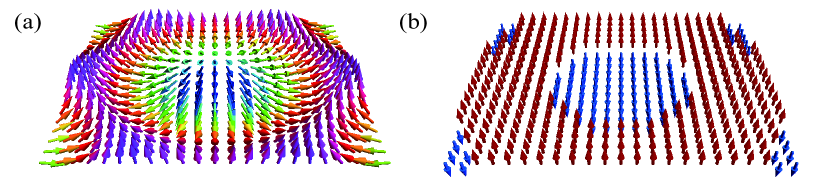
Figure 1: (Color online) Schematic views of (a) a noncoplanar skyrmion texture and (b) a collinear bubble. Triangular crystals of these structures are induced by magnetic field and easy-axis anisotropy in high-symmetry frustrated magnets.

II Model

We consider a frustrated Heisenberg model on a TL:

$$\mathcal{H}=\sum_{\langle i,j\rangle}J_{ij}\mathbf{S}_{i}\cdot\mathbf{S}_{j}-H\sum_{i}S^{z}_{i}-A\sum_{i}(S^{z}_{i})^{2}.$$ (1)

The classical moments, $\mathbf{S}_{i}$, have a fixed magnitude $\mathbf{S}_{i}^{2}=1$. The first term is the isotropic exchange interaction, including nearest-, second nearest-, and third nearest-neighbor couplings, $J_{1}$, $J_{2}$, and $J_{3}$, respectively. The ferromagnetic interaction, $J_{1}=-1$, will be our unit of energy and the lattice constant, $a$, will be adopted as the unit of length. Frustration arises from the antiferromagnetic nature of the further neighbor interactions $J_{2}>0$ and $J_{3}>0$. The second and third terms represent the Zeeman coupling to an external magnetic field and the easy-axis ($A>0$) spin anisotropy, respectively. $\mathcal{H}$ is invariant under the space-group of the TL and under the U(1) group of global spin rotations along the field-axis.

Below the saturation field, $H_{\rm sat}$, the ground state of $\mathcal{H}(A=0)$ is the conical spiral: $\mathbf{S}_{i}=(\sin\theta\cos(\mathbf{Q}\cdot\mathbf{r}_{i}),\ \sin\theta\sin(\mathbf{Q}\cdot\mathbf{r}_{i}),\ \cos\theta)$ with $Q=|\mathbf{Q}|=(2/\sqrt{3})\cos^{-1}\left[(1+J_{1}/J_{2})/2\right]$ for the $J_{1}$-$J_{2}$ model ($J_{3}=0$) and $Q=2\cos^{-1}\left[(1+\sqrt{1-2J_{1}/J_{3}})/4\right]$ for the $J_{1}$-$J_{3}$ model ($J_{2}=0$). In each case there are six possible ordering wave-vectors, $\pm{\bf Q}_{\nu}$ $({\nu=1,2,3})$, because of the C₆ symmetry of the TL. These vectors are parallel to the nearest (next-nearest) neighbor bond directions for the $J_{1}$-$J_{3}$ ($J_{1}$-$J_{2}$) model. The canting angle $\theta$ is given by $\cos\theta=H/H_{\rm sat}$ with $H_{\rm sat}=J(\mathbf{Q})-J(\mathbf{0}),$ and $J(\mathbf{q})=\sum_{\bm{\delta}}J_{\bm{\delta}}e^{i{\bf q}\cdot\bm{\delta}}$ (${\bm{\delta}}$ is the relative vector between neighboring sites). From this relationship, we obtain that $H_{\rm sat}\propto Q^{4}$ for $Q\ll 1$, i.e., near the Lifshitz transition to the commensurate $Q=0$ ferromagnetic state.

III Isotropic Spin Interactions

We start by considering isotropic spin interactions ($A=0$) in order to isolate the effect of the six-fold lattice anisotropy. This anisotropy appears upon expanding $J(\mathbf{q})$ up to sixth order in $q_{x}$ and $q_{y}$. For the $J_{1}$-$J_{3}$ model we have

$$J(\mathbf{q})= - 6(J_{1}+J_{3})+\frac{3}{2}(J_{1}+4J_{3})q^{2}-\frac{3}{32}(J_{1}+16J_{3})q^{4}$$

$$+ \frac{1}{384}(J_{1}+64J_{3})q^{6}+\frac{1}{3840}(J_{1}+64J_{3})q^{6}\cos 6\phi,$$

where $\mathbf{q}=(q\cos\phi,q\sin\phi)$.

The thermodynamic phase diagram of the $J_{1}$-$J_{2}$ and the $J_{1}$-$J_{3}$ is obtained from unbiased MC simulations based on the Metropolis algorithm and the over-relaxation method. The lattices used for these simulations have $N=L^{2}$ spins and periodic boundary conditions. The target temperature is reached by simulated annealing over $10^{5}$-$10^{6}$ MC sweeps (MCS) and $10^{5}$-$10^{7}$ MCS measurements are performed after equilibration. Statistical errors are estimated by taking averages over $3$-$16$ independent runs.

According to our MC simulation of ${\cal H}$ on $L=75$, $98$, $100$ $120$ lattices, the conical spiral is the only ordered phase for small enough $Q$. For the $J_{1}$-$J_{3}$ model, the skyrmion crystal phase only appears above $Q^{\rm c}=1.980(4)$, which corresponds to $J_{2}^{\rm c}/|J_{1}|=1.4027(138)$. For the $J_{1}$-$J_{3}$ model, we obtain $Q^{\rm c}=1.648(2)$, which corresponds to $J_{3}^{\rm c}/|J_{1}|=1.0256(53)$. These results indicate that the locking potential, which grows as $Q^{6}$ and forces three helices to propagate along the principal axes of the TL, has to reach a critical value to stabilize the skyrmion crystal phase in isotropic magnets. As we will see in the next sections, this condition is no longer required in the presence of a moderate easy-axis anisotropy.

IV Multi-$\mathbf{Q}$ Instability Induced by a Single-Ion Anisotropy

The purpose of this Section is to demonstrate that a finite easy-axis anisotropy is enough to stabilize multi-${\bf Q}$ orderings. To this end we will perform a stability analysis of the single-${\bf Q}$ conical spiral phase based on the following deformation: 

$$S^{x}_{j} = \sqrt{\sin^{2}{\!\tilde{\theta}}-\Delta^{2}_{2}}\cos{({\bf Q}_{1}\cdot{\bf r}_{j})}+\Delta_{2}\cos{({\bf Q}_{2}\cdot{\bf r}_{j})},$$

$$S^{y}_{j} = \sqrt{\sin^{2}{\!\tilde{\theta}}-\Delta^{2}_{2}}\sin{({\bf Q}_{1}\cdot{\bf r}_{j})}-\Delta_{2}\sin{({\bf Q}_{2}\cdot{\bf r}_{j})},$$

$$S^{z}_{j} = \sqrt{\cos^{2}{\!\tilde{\theta}}-2\Delta_{2}\sqrt{\sin^{2}{\!\tilde{\theta}}-\Delta^{2}_{2}}\cos{{\bf Q}_{3}}\cdot{\bf r}_{j}},$$ (3)

where the amplitude of the ${\bf Q}_{2}$ component, $\Delta_{2}$, is a variational parameter and $\cos{\tilde{\theta}}$ is determined below [see Eq. (8)].

We will demonstrate that the energy of the variational state given in Eq. (3) is a decreasing function of $\Delta_{2}$ for $\Delta_{2}\ll 1$. This means that the single-${\bf Q}_{1}$ conical state ($\Delta_{2}$=0) is unstable towards the development of a second ${\bf Q}_{2}$ component, as long as the magnetic field, $H$, and the easy-axis anisotropy, $A$, are non-zero. We will then expand the total energy per site, $E(\Delta_{2})$, to fourth order in $\Delta_{2}$. In general, the total energy per site of an arbitrary state is given by

$$E=\langle\mathcal{H}\rangle=\frac{1}{N}\sum_{\bf q}J({\bf q})|\langle{\bf S}_{\bf q}\rangle|^{2}-\frac{H\langle S^{z}_{\bf 0}\rangle}{\sqrt{N}}-\frac{A}{N}\sum_{j}\langle(S^{z}_{j})^{2}\rangle,$$ (4)

with

$${\bf S}_{\bf q}=\frac{1}{\sqrt{N}}\sum_{j}{\bf S}_{j}e^{i{\bf q}\cdot{\bf r}_{j}}.$$ (5)

For the state under consideration, we have:

$$S^{z}_{j}=\cos{\tilde{\theta}}\left[1-x\cos{{\bf Q}_{3}\cdot{\bf r}_{j}}-\frac{x^{2}}{2}\cos^{2}{\!{\bf Q}_{3}\cdot{\bf r}_{j}}-\frac{x^{3}}{2}\cos^{3}{\!{\bf Q}_{3}\cdot{\bf r}_{j}}-\frac{5x^{4}}{8}\cos^{4}{\!{\bf Q}_{3}\cdot{\bf r}_{j}}+{\cal O}(\Delta^{5}_{2})\right],$$ (6)

with

$$x=\frac{\Delta_{2}}{\cos^{2}{\!\tilde{\theta}}}\sqrt{\sin^{2}{\!\tilde{\theta}}-\Delta^{2}_{2}}.$$ (7)

We will choose ${\tilde{\theta}}$, such that

$$\cos{\theta}\!=\!\cos{\tilde{\theta}}\;[1-\Delta^{2}_{2}(\sin^{2}{\!\tilde{\theta}}-\Delta^{2}_{2})/(4\cos^{4}{\!\tilde{\theta}})].$$ (8)

For this choice of ${\tilde{\theta}}$ we have:

$$\frac{|\langle S^{z}_{\bf 0}\rangle|}{\sqrt{N}} = \cos{\theta}-\frac{15}{64}\cos{\tilde{\theta}}x^{4}+{\cal O}(\Delta^{5}_{2})$$

$$\frac{|\langle S^{z}_{{\bf Q}_{3}}\rangle|^{2}}{N} = \cos^{2}{\!\tilde{\theta}}\left[\frac{x^{2}}{2}+\frac{3x^{4}}{8}\right]+{\cal O}(\Delta^{6}_{2})$$

$$\frac{|\langle S^{z}_{2{\bf Q}_{3}}\rangle|^{2}}{N} = \cos^{2}{\!\tilde{\theta}}\frac{x^{4}}{32}+{\cal O}(\Delta^{6}_{2})$$

$$\sum_{\nu=1,2;\mu=x,y}\frac{|\langle S^{\mu}_{{\bf Q}_{\nu}}\rangle|^{2}}{N} = \sin^{2}{\!\tilde{\theta}}.$$ (9)

By adding the different contributions to Eq. (4), we obtain:

$$E(\Delta_{2})-E(\Delta_{2}=0) = \left[\frac{J(2{\bf Q}_{3})-J({\bf 0})}{32}+\frac{9A}{8}\right]x^{4}\cos^{2}{\!\tilde{\theta}}$$ (10)

$$- \frac{Ax^{2}}{2}\cos^{2}{\!\tilde{\theta}}+{\cal O}(\Delta^{5}_{2}),$$

where we have used that $H=2\cos{\tilde{\theta}}[J({\bf 0})-J({\bf Q}_{\nu})]$ to zeroth order in $\Delta_{2}$. It is clear from this expression that the energy is a decreasing function of $\Delta_{2}$ for small enough $\Delta_{2}$. In particular, if we assume that $A\ll J(2{\bf Q}_{3})-J({\bf 0})$, we can minimize (10) as a function of $x$ to obtain.

$$x^{2}=\frac{8A}{J(2{\bf Q}_{3})-J({\bf 0)}},$$ (11)

implying that

$$\Delta_{2}\simeq\frac{\cos^{2}{\theta}\sqrt{8A}}{\sin{\theta}\sqrt{J(2{\bf Q}_{3})-J({\bf 0)}}}.$$ (12)

Thus, we find that the single-${\bf Q}$ conical state is unstable toward the multi-${\bf Q}$ deformation. A key observation is that the modulation of the $z$ spin component, required to preserve the constraint ${\bf S}^{2}_{i}=1$, has a very small exchange energy cost in a C₆ invariant system: to linear order in $\Delta_{2}$, the $z$-component is modulated by the third wave-vector ${\bf Q}_{3}$, which still minimizes $J(\mathbf{q})$. This is so because the C₆ symmetry of the TL guarantees that ${\bf Q}_{1}+{\bf Q}_{2}+{\bf Q}_{3}=0$. Therefore, the exchange energy cost of the higher harmonics produced by the normalization condition is proportional to $\Delta_{2}^{4}[J(2{\bf Q}_{3})-J({\bf 0})]$, while the anisotropy energy gain produced by the same modulation is proportional to $-A\Delta^{2}_{2}$, as it is shown in Eq. (10). In the end, this leads to $\Delta_{2}\propto\sqrt{A/[J(2{\bf Q}_{3})-J({\bf 0})]}$ for $\Delta_{2}\ll 1$ or $A\ll|J(2{\bf Q}_{\nu})|$, as obtained in Eq. (12). Finally, it is interesting to note that a double-${\bf Q}$ conical state, like the one described by Eq. (3), has been obtained below the saturation field of a spatially anisotropic TL model Starykh et al. (2014).

V Small ${\bf Q}$

In Sec. III we showed that a critical $Q$-value is required to stabilize a skyrmion crystal for isotropic spin interactions. In Sec. IV, we demonstrated that a single-${\bf Q}$ conical spiral phase is unstable towards multi-${\bf Q}$ orderings in the presence of finite easy-axis anisotropy. It is then natural to ask what is the thermodynamic phase diagram for small $Q$-values ($Q<Q^{\rm c}$) as a function of magnetic field and easy-axis anisotropy $A$. This is the main purpose of this Section. We start with a simple $T=0$ variational analysis, which is complemented by finite-$T$ MC simulations.

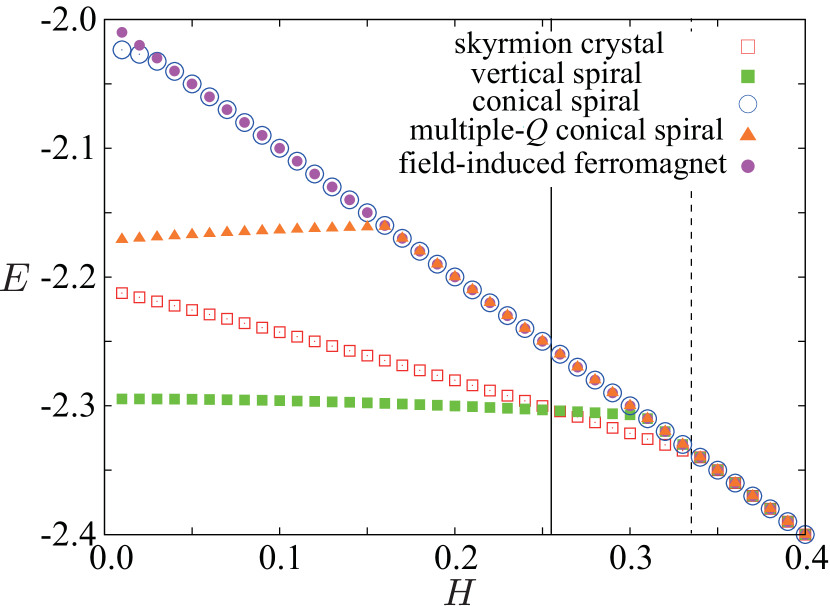
Figure 2: (Color online) $H$ dependence of the energy per site of different variational states for $Q=2\pi/5$ and $A=0.5$. The vertical solid line marks the phase boundary between the single-${\bf Q}$ vertical spiral and skyrmion crystal phases. The vertical dashed line marks the phase boundary between the skyrmion crystal and fully polarized state. Here we only considered the multiple-${\bf Q}$ conical spiral with $I_{x}=I_{y}$.

V.1 Variational Analysis

Here we present a simple $T=0$ variational analysis of the $J_{1}$-$J_{3}$ model based on the following variational states:

(1) Skyrmion crystal phase: the spin configuration is given by $\mathbf{S}=\mathbf{M}/|M|$, with

$${\bf M}^{x,y}_{i} = {I_{xy}}\sum_{\nu=1-3}\sin{({\bf Q}_{\nu}\cdot{\bf r}_{i}+\theta_{\nu})}\;\;{\bf e}_{\nu},$$

$$M^{z}_{i} = m_{z}-{I_{z}}\sum_{\nu=1-3}\cos{({\bf Q}_{\nu}\cdot{\bf r}_{i}+\theta_{\nu})}\;\;{\bf e}_{\nu}.$$ (13)

The three unit vectors are ${\bf e}_{1}={\hat{\bf x}}$, ${\bf e}_{2}=-{\hat{\bf x}}/2+\sqrt{3}{\hat{\bf x}}/2$, and ${\bf e}_{3}=-{\hat{\bf x}}/2-\sqrt{3}{\hat{\bf x}}/2$, $\mathbf{Q}_{\nu}=Q\mathbf{e}_{\nu}$ and $m_{z}$ is the uniform spin magnetization. Higher harmonics are generated by the normalization condition ${\bf S}^{2}_{i}=1$. Without loss of generality, we take $\theta_{\nu}=0$ because $\mathcal{H}$ is invariant under global spin rotations along the magnetic field direction. The variational parameters of the skyrmion crystal state (13) are $m_{z}$, $I_{z}$, $Q_{v}$ and $I_{xy}$.

(2) Fully polarized state:

$${\bf S}^{xy}_{i}=0,\;\;\;S^{z}_{i}=1.$$ (14)

(3) Single-$\bm{Q}$ conical spiral:

$${\bf S}^{xy}_{i} = \sqrt{1-m_{z}^{2}}\;\;[\cos{({\bf Q}_{\nu}\cdot{\bf r}_{i})}\;\;{\hat{\bf x}}+\sin{({\bf Q}_{\nu}\cdot{\bf r}_{i})}\;\;{\hat{\bf y}}],$$

$$S^{z}_{i} = m_{z}.$$ (15)

(4) Single-$\bm{Q}$ vertical spiral: the spin configuration is given by $\mathbf{S}=\mathbf{M}/|M|$, with

$${\bf M}^{xy}_{i} = {I_{xy}}\cos{({\bf Q}_{\nu}\cdot{\bf r}_{i})}\;\;{\hat{\bf x}},$$

$$M^{z}_{i} = m_{z}+{I_{z}}\sin{({\bf Q}_{\nu}\cdot{\bf r}_{i})},$$ (16)

where we have assumed that the spins rotate in the $x$-$z$ plane. Once again, the orientation of this polarization plane is arbitrary (provided it is parallel to the $z$-axis) because $\mathcal{H}$ is U(1) invariant under global spin rotations along the $z$-axis.

(5) Multiple-$\bm{Q}$ conical spiral: this state corresponds to Eq. (3) and it is given by $\mathbf{S}=\mathbf{M}/|M|$ with

$$M^{x}_{i} = {I_{x}}[\cos{({\bf Q}_{1}\cdot{\bf r}_{i})}+\cos{({\bf Q}_{2}\cdot{\bf r}_{i})}],$$

$$M^{y}_{i} = {I_{y}}[\sin{({\bf Q}_{1}\cdot{\bf r}_{i})}-\sin{({\bf Q}_{2}\cdot{\bf r}_{i})}],$$

$$M^{z}_{i} = m_{z}+{I_{z}}\cos({\bf Q}_{3}\cdot{\bf r}_{i}).$$ (17)

As it can be inferred from the analysis of Eqs. (3) and (12), this state has lower energy than that of the single-${\bf Q}$ conical state for finite $A$ and $H$. Leonov and Mostovoy (2015)

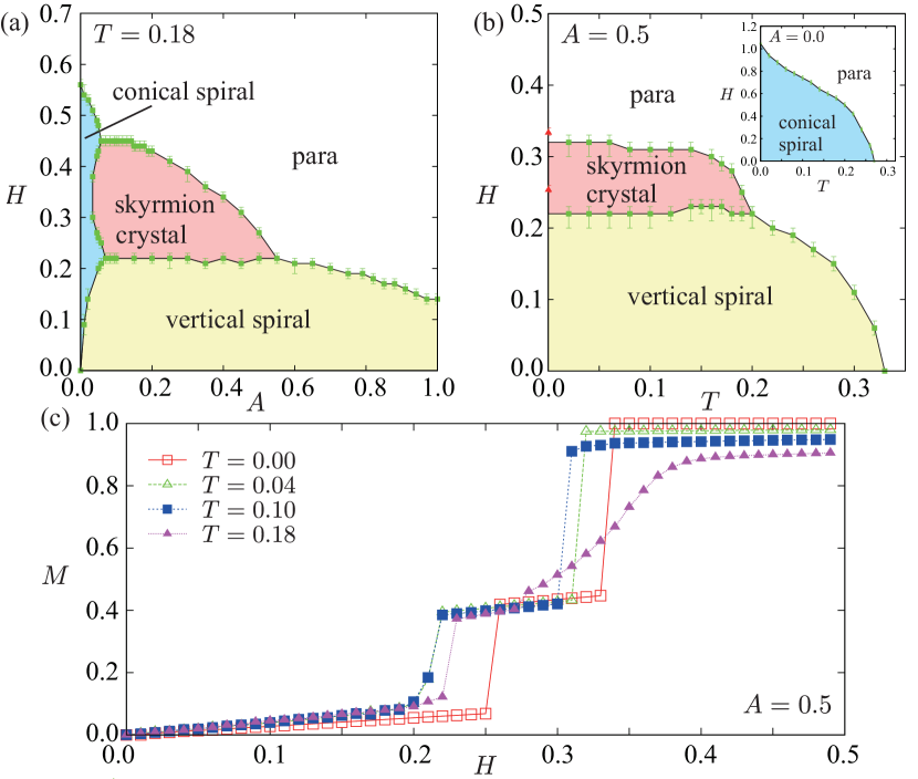
Figure 3: (Color online) (a) $A$-$H$ phase diagram obtained from MC simulations of the $J_{1}$-$J_{3}$ model for $J_{3}/|J_{1}|=0.5$ at $T=0.18$. (b) $T$-$H$ phase diagram for $A=0.5$ . The red triangles are determined from $T=0.0$ variational calculations. The inset shows the phase diagram for $A=0.0$. (c) Field dependence of the magnetization at different temperatures for $A=0.5$. The error bars are smaller than the symbol size.

Figure 2 shows the $H$-dependence of the energy density of each variational state for $Q=2\pi/5$ ($J_{3}/|J_{1}|=0.5$) and $A=0.5$. The vertical spiral, skyrmion crystal, and fully-polarized states become stable upon increasing $H$. For strong enough anisotropy $A$, the vertical spiral can continuously reduce the width of the domain wall between spin up and down domains through the development of higher harmonics. This is the reason why the vertical spiral has lower energy than the conical spiral state. While the multiple-${\bf Q}$ conical spiral is not the global energy minimum for this set of parameters, it always has lower energy than the single-${\bf Q}$ conical spiral. Moreover, in agreement with the variational analysis of Eq. (3) in Sec. IV, the multiple-${\bf Q}$ conical spiral becomes the ground state for a small values of $A\ll 1$. Leonov and Mostovoy (2015)

V.2 Monte Carlo Simulations

The MC phase diagrams are obtained by computing the uniform spin susceptibility, specific heat, and the spin and chiral structure factors,

$$S^{\nu\nu}_{s}({\bf q}) = \frac{1}{N}\sum_{j,l}\langle S^{\nu}_{j}S^{\nu}_{l}\rangle e^{i{\bf q}\cdot({\bf r}_{j}-{\bf r}_{l})},$$

$$S_{\chi}^{\mu\mu}({\bf q}) = \frac{1}{N}\sum_{\gamma,\eta}\langle\chi^{\mu}_{\gamma}\chi^{\mu}_{\eta}\rangle e^{i{\bf q}\cdot({\bf r}_{\gamma}-{\bf r}_{\eta})},$$ (18)

as a function of $H$, $A$ and $T$. The greek labels $\gamma$ and $\eta$ denote the sites of the dual (honeycomb) lattice of the TL. The brackets $\langle\cdots\rangle$ denote the thermodynamic average. $\chi^{\mu}_{\gamma}={\bf S}_{j}\cdot{\bf S}_{k}\times{\bf S}_{l}$ is the scalar chirality on the $\mu=u,d$ (up or down) triangle $jkl$ with center ${\bf r}_{\gamma}$.

Figure 3(a) shows the $A$-$H$ phase diagram of the $J_{1}$-$J_{3}$ model for $L=100$, $J_{3}/|J_{1}|=0.5$ and $T=0.18$. A conical spiral phase appears for small $A$. In agreement with our variational analysis of Eq. (3) and direct variational calculations in Fig. 2, this phase becomes unstable at lower temperatures. The vertical spiral phase is induced at low-fields. This phase is not a pure single-${\bf Q}$ ordering because of higher harmonics induced by $A$: the optimal vertical spiral is elliptical instead of circular to have the spins more aligned with the easy-axis. The real-spin configuration and the spin structure factor of the vertical spiral are shown in Fig. 4. As we will discuss in Sec. VI, for larger $A$ values this elliptical distortion eventually evolves into a “collinear 1D” phase, which preserves the 1D modulation of the spiral phase.

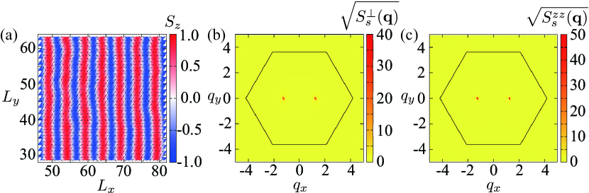
Figure 4: (Color online) Snapshots of spin configurations and the corresponding spin structure factor of the vertical spiral appearing in Fig. 3(b) for $Q=2\pi/5$ and $N=100\times 100$. The data are taken for $A=0.5$, $H=0.15$, and $T=0.15$. In (a), we average over $500$ MCS to integrate out the short wavelength fluctuations. Panels (b) and (c) show the square root of the $xy$ and $z$ components of the spin structure factor, respectively. Here and hereafter, the field-induced $\mathbf{q}=0$ component is subtracted for clarity.

The skyrmion crystal phase emerges at intermediate magnetic field values and above a rather small critical $A$ value. This phase narrows down with increasing $A$ because the easy-axis anisotropy naturally favors the fully polarized state ($H_{\rm sat}$ decreases with $A$). Except for the second-order phase transition between the conical spiral and the fully polarized state, the other transitions are of first order, as it is clear from the discontinuities in the magnetization curves, $M(H)$, shown in Fig. 3(c). We also note that the magnetization curve has a very small slope ($M\sim 0.4$) inside the skyrmion crystal phase.

Figure 5(a) shows a typical real space spin configuration obtained from a snapshot of the MC simulation in the skyrmion crystal phase. The skyrmion cores (blue regions) form a triangular crystal with lattice parameter $4\pi/(\sqrt{3}Q)\sim 5.77$. The snapshot of the local scalar chirality, $\chi^{\mu}_{jkl}={\bf S}_{j}\cdot{\bf S}_{k}\times{\bf S}_{l}$, shown in Fig. 5(b), indicates that this phase has a net uniform scalar chirality, $\bar{\chi}=\sum_{\langle ijk\rangle}\chi_{ijk}/N$, as expected for a SC. This is confirmed by our finite size scaling analysis of the chiral structure factor in Appendix A. The six peaks in both $S_{s}^{\perp}$ and $S_{s}^{zz}$ [see Figs. 5(c) and 5(d)] indicate the formation of a triangular SC. Note that $S_{s}^{\perp}$ can only order at $T=0$ in 2D, Mermin and Wagner (1966) while $S_{s}^{zz}$ can exhibit sharp Bragg peaks at finite-$T$ because the wave-vectors ${\bf Q}_{\nu}$ are commensurate with the underlying TL.

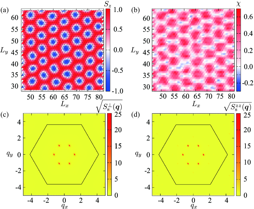
Figure 5: (Color online) Snapshot of the real-space (a) spin configuration and (b) scalar chirality in the skyrmion crystal phase for $H=0.27$ and $T=0.15$ in Fig. 3(b). The color scale in (a) indicates the $z$ spin component, parallel to $H$, while the arrows indicate the in-plane $xy$ components. The lattice size is $L=100$ and the MC results are obtained after averaging over $500$ MCS. Panels (c) and (d) show the $xy$ and $z$ components of the spin structure factor, respectively.

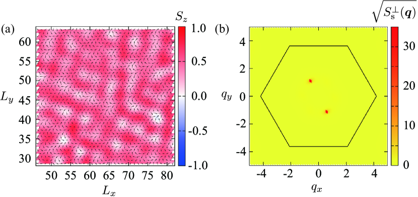
Figure 6: (Color online) (a) Snapshot of the spin configurations and (b) the square root of the $xy$ component of the spin structure factor for the conical spiral phase in Fig. 3(a). The Hamiltonian parameters are $Q=2\pi/5$, $A=0.02$, $H=0.43$, $T=0.18$ and the lattice size is $N=75\times 75$. The snapshot of the spin configuration in (a) is obtained after averaging over $2000$ MCS in order to integrate out the short wavelength fluctuations. The field-induced $\mathbf{q}=0$ component of the spin structure factor has been omitted in (b). Note that the $z$-spin component remains uniform in the conical spiral state.

The real space spin configurations of the other two phases, the single-${\bf Q}$ conical and vertical spirals, are shown Figs. 4 and 6, respectively. It is interesting to compare the finite temperature MC phase diagram shown in Fig. 3(a) with the $T=0$ variational phase diagram reported in Ref. Leonov and Mostovoy, 2015. As shown in Fig. 3(a), the single-${\bf Q}$ conical state and the single-${\bf Q}$ vertical spiral are the only ordered states at $T=0.18$ for small $H$ and $A$. As shown in Fig. 7 our Monte Carlo results indicate that these single-${\bf Q}$ states evolve into multiple-${\bf Q}$ states upon lowering the temperature. This behavior is consistent with the $T=0$ variational calculations of Ref.  Leonov and Mostovoy, 2015. However, it is important to emphasize that the phase diagram becomes qualitatively different in the presence of moderate thermal fluctuations. Indeed, at low enough temperatures the single-${\bf Q}_{1}$ vertical spiral becomes unstable over a finite field interval towards a finite spin modulation in the direction perpendicular to the original spin polarization plane. As it is shown in Figs. 7 (a-c), this additional spin modulation has equal intensity for the ${\bf Q}_{2}$ and ${\bf Q}_{3}$ components. In addition, the single-${\bf Q}$ conical spiral state becomes a multiple-${\bf Q}$ conical spiral upon lowering the temperature, in agreement with the analysis presented in Sec. IV [see Figs. 7 (d-i)].

The phase diagram of Fig. 3(a) also exhibits a field-induced transition between the vertical spiral and the skyrmion crystal phase for larger values of $A$. This transition can be interpreted in the following way. When $A$ becomes a significant fraction of $|J_{1}|$, the crossover between the spin down and up regions of a low-energy spin configuration occurs over length scale of order $\sqrt{J_{1}/A}$. This length can be made much shorter than $2\pi/Q$ in the long wave length limit $Q\ll 1$, i.e., we can assume that the boundary between domains with opposite spin alignment is a line with positive tension. The energy of a given state can then be reduced by minimizing the perimeter of the boundary per unit of area. The effect of $H$ on the vertical spiral is to move the up-down boundaries to the right and the down-up boundaries to the left in order to shrink (expand) the spin down (up) stripes. This implies that the perimeter per unit of area, $P_{h}/A_{h}=Q/\pi$, does not depend on the value of the uniform magnetization $M$ along the field direction. In contrast, the perimeter per unit area of the SC, $P_{s}/A_{s}=3^{1/4}Q\sqrt{1-M}/2\sqrt{\pi}$, does depend on $M$ because the skyrmion cores shrink as a function of $H$. We then expect a transition from the vertical spiral to the skyrmion crystal state when $P_{h}/A_{h}\approx P_{s}/A_{s}$, which leads to a critical value of $M_{\rm c}\simeq 0.265$. Given that the transition between both phases is of first order, we need to consider the average between the $M$ values right below and above the transition. According to the results shown in Fig. 3(c), this average is $0.24$, which is in good agreement with our simple estimate.

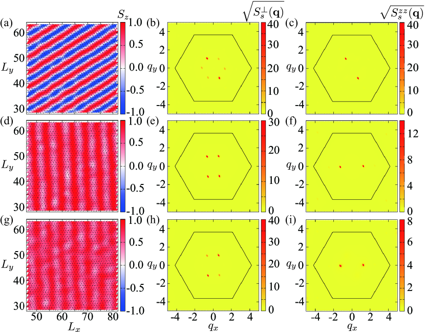
Figure 7: (Color online) Snapshots of spin configurations and the square root of the spin structure factor for $Q=2\pi/5$, $T=0.02$ and $N=75\times 75$ spins. (a)-(c) Multiple-${\bf Q}$ vertical spiral obtained for $A=0.03$ and $H=0.19$, (d)-(f) multiple-${\bf Q}$ conical spiral with equal transverse amplitudes, $I_{x}=I_{y}$, obtained for $A=0.05$ and $H=0.64$, and (g)-(i) Multiple-${\bf Q}$ conical spiral with different transverse amplitudes, $I_{x}\neq I_{y}$, obtained for $A=0.02$ and $H=0.67$.

Finally, it is also interesting to study the evolution of the finite-$T$ phase diagram towards $T=0$ when $A$ is comparable to $|J_{1}|$. Figure 3(b) shows the $T$-$H$ phase diagram for $L=100$, $J_{3}/|J_{1}|=0.5$ and $A=0.5$. The MC results are complemented with $T=0$ variational calculations in Fig. 2, whose phase boundaries, denoted with red triangles in Fig. 3(c), deviate slightly from the $T\to 0$ extrapolation of the MC results. The skyrmion crystal phase extends all the way to $T=0$, in agreement with the variational treatment of Ref. Leonov and Mostovoy, 2015.

VI Large-$\mathbf{Q}$

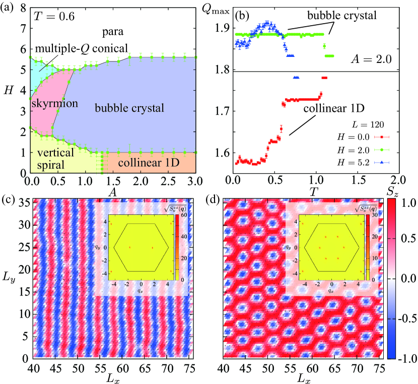
Figure 8: (Color online) (a) $A$-$H$ phase diagram of the $J_{1}$-$J_{3}$ model at $T=0.60$ and for $Q=4\pi/7$ ($J_{3}\sim 1.62$). (b) $T$-dependence of the ordering-vectors of the collinear 1D and BC phases ($A=2.0$). The horizontal line corresponds to $Q=4\pi/7$. Panels (c) and (d) show typical spin configurations for the collinear 1D and BC phases, respectively. The insets of panels (c) and (d) show $S^{zz}_{s}$.

In this Section we will study the effect of easy-axis spin anisotropy in the large-${\bf Q}$ regime by considering the $J_{1}$-$J_{3}$ model with $Q=4\pi/7$ ($J_{3}\sim 1.62$). Figure 8(a) shows the typical $A$-$H$ phase diagram at intermediate $T$-values ($T=0.60$) obtained from simulations on lattices of $N=98\times 98$ spins. Four phases appear in the small $A$ region: vertical spiral, SC, multiple-${\bf Q}$ conical, and paramagnetic states. The vertical spiral and the skyrmion crystal phases are similar to the ones already described for small-$Q$ [see Figs. 4 and 5]. A typical spin configuration for multiple-${\bf Q}$ conical state is shown in Fig. 9.

Remarkably, the large $A$ region includes two collinear broken symmetry states. The low-field phase corresponds to a spin density wave with a 1D modulation, as it is clear from real-space spin configuration shown in Fig. 8(c) and from the longitudinal spin structure factor, $S^{zz}_{s}$, shown in the inset of the same figure. In contrast, the high-field collinear BC phase, schematically displayed in Fig.1(b), is modulated along three principal directions parallel to the vectors ${\bf Q}_{\nu}$ [see Fig. 8(d) and its inset]. Similar BC phases have been previously discussed in different contexts. Bobeck and Scovil (1971); Thiele (1973); Seshadri and Westervelt (1991) The local scalar chirality induced by thermal fluctuations near the phase boundary between the skyrmion and the bubble crystals decreases gradually and disappears for increasing $A$. Consistently with this behavior, $S^{\perp}_{s}$ exhibits quasi-long range ordering in the finite-$T$ skyrmon crystal phase and only short range correlations in the bubble crystal phase.

Another interesting aspect of the collinear phases is the temperature dependence of their spatial modulation, similar to the well-known case of the axial next-nearest-neighbor Ising (ANNNI) model. Elliott (1961); Fisher and Selke (1980); Selke (1988) We note that in both cases there is a competition between frustrated exchange couplings and easy-axis anisotropy. Moreover, the low-field collinear state of Fig. 8(a) exhibits a spontaneous 1D modulation similar to the case of the ANNNI model. As expected, the dominant ordering wave-vector of the low-field collinear phase (obtained from the peak position of $S^{zz}_{s}({\bf q})$) exhibits plateaus of different sizes and a quasi-continuous behavior in between [see bottom of Figure 8(b)], which is very similar to the result for the ANNNI model. Selke (1988)

The BC phase can be regarded as a multi-${\bf Q}$ extension of the ANNNI physics. The bubble density increases with decreasing temperature, as shown in Fig. 8(b) for $H=2.0$ and $5.2$. Once again, the competition between exchange and anisotropy induces temperature driven commensurate-incommensurate transitions. In all cases, the ordering wave-vector evolves towards the $Q$-value selected by the competing exchange interactions (largest magnetic susceptibility) upon approaching the transition to the paramagnetic state (see horizontal line in Fig. 8(b)). However, the moments become longitudinally rigid upon decreasing temperature forcing the dominant ordering vector to deviate from the optimal $Q$-value at $T=T_{c}$.

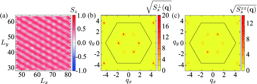
Figure 9: (Color online) (a) Snapshot of spin configuration and (b)-(c) the square root of the spin structure factor of the multiple-${\bf Q}$ conical spiral in Fig. 8(a). The Hamiltonian parameters are $Q=2\pi/5$, $A=0.2$, $H=4.4$, $T=0.6$ and the system size is $N=75\times 75$. The snapshot of the spin configuration in (a) is obtained after averaging over $500$ MCS to integrate out the short wavelength fluctuations. The field-induced $\mathbf{q}=0$ component of the structure factor has been omitted in (b) and (c).

VII Summary

In summary, we found that both spatial and easy-axis spin anisotropies stabilize magnetic field-induced skyrmion crystals in frustrated magnets. Strong six-fold spatial anisotropy induced by a large ordering wave-vector is enough to stabilize a finite temperature skyrmion crystal in isotropic (Heisenberg) frustrated TL magnets. However, a small easy-axis anisotropy is required to render the skyrmion crystal stable in the long wave length limit. The universality of this continuum limit implies that the same is true for any $C_{6}$ invariant frustrated lattice model, such as honeycomb or Kagome. Moreover, our variational argument based on Eq. (3), which holds for arbitrary $Q$, is also valid for any $C_{6}$ invariant lattice. The skyrmion crystal phase is replaced by a collinear crystal of magnetic bubbles for strong enough spatial and easy-axis anisotropies.

Our study underscores the rich multiple-${\bf Q}$ spin textures that emerge from the combination of frustration and anisotropy. The following three ingredients are enough to obtain field-induced multiple-${\bf Q}$ ordering: (1) $C_{6}$ symmetry szl , (2) finite $|{\bf Q}|$ ordering due to competing interactions, and (3) easy-axis anisotropy. Fe_xNi_1-xBr₂, Moore and Day (1985) Zn_xNi_1-xBr₂, Day et al. (1981) and an Fe monolayer on Ir(111) von Bergmann et al. (2006); Heinze et al. (2011) are then candidate materials to exhibit field-induced skyrmion crystal or BC phases.

Appendix A Finite-size Scaling of the Skyrmion Crystal and Other Phases

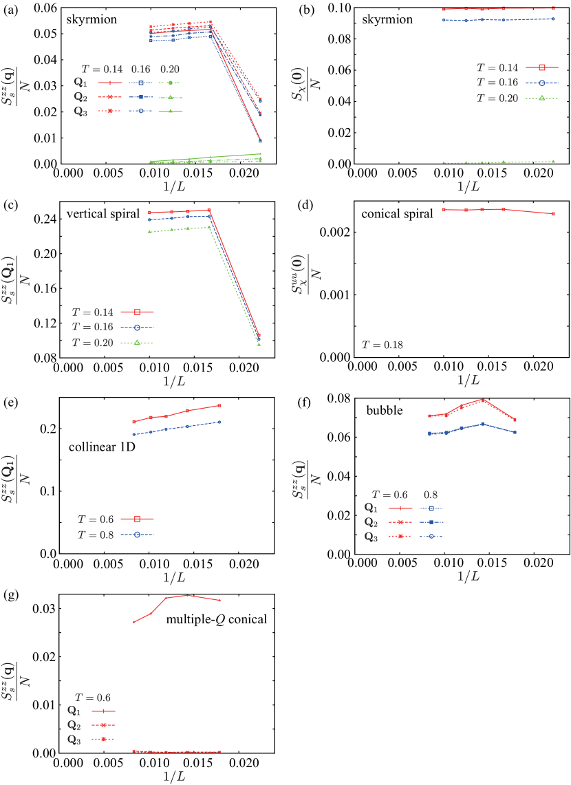
Figure 10: (Color online) Size dependence of the order parameters for each phase: (a) $z$-component of the spin structure factor evaluated at $\mathbf{q}=\mathbf{Q}_{1},\mathbf{Q}_{2},\mathbf{Q}_{3}$ and (b) chirality structure factor evaluated at $\mathbf{q}=\mathbf{0}$ ($S_{\chi}(\mathbf{q})=S_{\chi}^{uu}(\mathbf{q})+S_{\chi}^{dd}(\mathbf{q})$) for $Q=2\pi/5$, $H=0.25$, $A=0.5$, and different temperatures in the skyrmion crystal phase; (c) $z$-component of the spin structure factor evaluated at $\mathbf{q}=\mathbf{Q}_{1}$ for $Q=2\pi/5$, $H=0.0$, $A=0.5$ in the vertical spiral state; (d) chirality structure factor for the upward triangles of the triangular lattice evaluated at $\mathbf{q}=\mathbf{0}$ for $Q=2\pi/5$, $H=0.4$ and $A=0.02$ in the conical spiral state; (e) $z$-component of the spin structure factor with $\mathbf{q}=\mathbf{Q}_{1}$ for $Q=4\pi/7$, $H=0.0$, and $A=2.0$ in the collinear 1D state; (f) $z$-component of the spin structure factor evaluated at $\mathbf{q}=\mathbf{Q}_{1},\mathbf{Q}_{2},\mathbf{Q}_{3}$ for $Q=4\pi/7$, $H=2.0$ and $A=2.0$ in the bubble crystal phase; (g) $z$-component of the spin structure factor evaluated at $\mathbf{q}=\mathbf{Q}_{1},\mathbf{Q}_{2},\mathbf{Q}_{3}$ for $Q=4\pi/7$, $H=4.4$ and $A=0.2$ in the multiple-${\bf Q}$ conical state.

In this Appendix we include a finite-size scaling analysis of each phase of the phase diagram shown in Figs. 3 and 8. Figures 10(a) and 10(b) include the $1/L$ dependence of the $z$-component of the spin structure factor and the uniform scalar chirality normalized by the system size $N$ in the skyrmion crystal phase. As expected, the 3-${\bf Q}_{\nu}$ ($\nu=1,2,3$) components of $S^{zz}_{s}({\bf q})$ extrapolate to a finite value in the thermodynamic limit ($L\to\infty$). The same is true for the uniform scalar spin chirality. We also show the finite size scaling analysis for other phases included in Figs. 10. Panels (c)-(g) include the vertical spiral in Fig. 3(b), the conical spiral in Fig. 3(a), the collinear 1D phase in Fig. 8(a), the bubble crystal in Fig. 8(a) and the multiple-${\bf Q}$ conical spiral in Fig. 8(a) of the main text, respectively.

References

- Yoshimori (1959) A. Yoshimori, J. Phys. Soc. Jpn. 14, 807 (1959).
- Kaplan (1961) T. A. Kaplan, Phys. Rev. 124, 329 (1961).
- Elliott (1961) R. J. Elliott, Phys. Rev. 124, 346 (1961).
- Ruderman and Kittel (1954) M. A. Ruderman and C. Kittel, Phys. Rev. 96, 99 (1954).
- Kasuya (1956) T. Kasuya, Prog. Theor. Phys. 16, 45 (1956).
- Yosida (1957) K. Yosida, Phys. Rev. 106, 893 (1957).
- Martin and Batista (2008) I. Martin and C. D. Batista, Phys. Rev. Lett. 101, 156402 (2008).
- Akagi and Motome (2010) Y. Akagi and Y. Motome, J. Phys. Soc. Jpn. 79, 083711 (2010).
- Kato et al. (2010) Y. Kato, I. Martin, and C. D. Batista, Phys. Rev. Lett. 105, 266405 (2010).
- Akagi et al. (2012) Y. Akagi, M. Udagawa, and Y. Motome, Phys. Rev. Lett. 108, 096401 (2012).
- Barros and Kato (2013) K. Barros and Y. Kato, Phys. Rev. B 88, 235101 (2013).
- Hayami and Motome (2014) S. Hayami and Y. Motome, Phys. Rev. B 90, 060402 (2014).
- (13) R. Ozawa, S. Hayami, K. Barros, G.-W. Chern, Y. Motome, and C. D. Batista, arXiv:1510.06830.
- Nakatsuji et al. (2005) S. Nakatsuji, Y. Nambu, H. Tonomura, O. Sakai, S. Jonas, C. Broholm, H. Tsunetsugu, Y. Qiu, and Y. Maeno, Science 309, 1697 (2005).
- Régnault, L.P. et al. (1982) Régnault, L.P., Rossat-Mignod, J., Adam, A., Billerey, D., and Terrier, C., J. Phys. France 43, 1283 (1982).
- Day et al. (1981) P. Day, M. W. Moore, C. Wilkinson, and K. R. A. Ziebeck, Journal of Physics C: Solid State Physics 14, 3423 (1981).
- Garel and Doniach (1982) T. Garel and S. Doniach, Phys. Rev. B 26, 325 (1982).
- Okubo et al. (2012) T. Okubo, S. Chung, and H. Kawamura, Phys. Rev. Lett. 108, 017206 (2012).
- Bogdanov and Yablonskii (1989) A. N. Bogdanov and D. A. Yablonskii, Sov. Phys. JETP 68, 101 (1989).
- Bogdanov and Hubert (1994) A. Bogdanov and A. Hubert, Journal of Magnetism and Magnetic Materials 138, 255 (1994), ISSN 0304-8853.
- Rößler et al. (2006) U. Rößler, A. Bogdanov, and C. Pfleiderer, Nature 442, 797 (2006).
- Leonov and Mostovoy (2015) A. O. Leonov and M. Mostovoy, Nature Communications 6, 8275 (2015).
- Lin and Hayami (2016) S.-Z. Lin and S. Hayami, Phys. Rev. B 93, 064430 (2016).
- Kamiya and Batista (2014) Y. Kamiya and C. D. Batista, Phys. Rev. X 4, 011023 (2014).
- Wang et al. (2015) Z. Wang, Y. Kamiya, A. H. Nevidomskyy, and C. D. Batista, Phys. Rev. Lett. 115, 107201 (2015).
- (26) L. Seabra, P. Sindzingre, T. Momoi, and N. Shannon, arXiv:1509.03850.
- Note (1) Note1, ref. 22 provides a similar argument but only for the continuum limit ().
- Starykh et al. (2014) O. A. Starykh, W. Jin, and A. V. Chubukov, Phys. Rev. Lett. 113, 087204 (2014).
- Mermin and Wagner (1966) N. D. Mermin and H. Wagner, Phys. Rev. Lett. 17, 1133 (1966).
- Bobeck and Scovil (1971) A. H. Bobeck and H. Scovil, Scientific American 224, 78 (1971).
- Thiele (1973) A. A. Thiele, Phys. Rev. Lett. 30, 230 (1973).
- Seshadri and Westervelt (1991) R. Seshadri and R. M. Westervelt, Phys. Rev. Lett. 66, 2774 (1991).
- Fisher and Selke (1980) M. E. Fisher and W. Selke, Phys. Rev. Lett. 44, 1502 (1980).
- Selke (1988) W. Selke, Physics Reports 170, 213 (1988).
- (35) Skyrmion crystals can also be stabilized in invariant lattices with easy-axis anisotropy as long as the spatial anisotropy is weak enough. See Ref. [23].
- Moore and Day (1985) M. W. Moore and P. Day, Journal of solid state chemistry 59, 23 (1985).
- von Bergmann et al. (2006) K. von Bergmann, S. Heinze, M. Bode, E. Y. Vedmedenko, G. Bihlmayer, S. Blügel, and R. Wiesendanger, Phys. Rev. Lett. 96, 167203 (2006).
- Heinze et al. (2011) S. Heinze, K. von Bergmann, M. Menzel, J. Brede, A. Kubetzka, R. Wiesendanger, G. Bihlmayer, and S. Blügel, Nature Physics 7, 713 (2011).