Mode instabilities and dynamic patterns in a colony of self-propelled surfactant particles covering a thin liquid layer.

Abstract

We consider a colony of point-like self-propelled surfactant particles (swimmers) without direct interactions that cover a thin liquid layer on a solid support. Although the particles predominantly swim normal to the free film surface, their motion also has a component parallel to the film surface. The coupled dynamics of the swimmer density and film height profile is captured in a long-wave model allowing for diffusive and convective transport of the swimmers (including rotational diffusion). The dynamics of the film height profile is determined by three physical effects: the upward pushing force of the swimmers onto the liquid-gas interface that always destabilizes the flat film, the solutal Marangoni force due to gradients in the swimmer concentration that always acts stabilising, and finally the rotational diffusion of the swimmers together with the in-plance active motion that acts either stabilising or destabilising. After reviewing and extending the analysis of the linear stability of the flat film with uniform swimmer density, we analyse the full nonlinear dynamic equations and show that point-like swimmers, which only interact via long-wave deformations of the liquid film, self-organise in highly regular (standing, travelling and modulated waves) and various irregular patterns for swimmer density and film height.

I Introduction

The self-assembly and self-organization of large numbers of microorganisms and artificial microswimmers and the non-equilibrium phase transitions that result from their collective behaviour have recently become the focus of many theoretical and experimental studies Ramaswamy (2010); Marchetti et al. (2013). Thus, in a series of experiments, carried out with different types of artificial microswimmers, several collective phenomena have been reported such as dynamic clustering, phase separation, and swarming Buttinoni et al. (2013); Theurkauff et al. (2012); Palacci et al. (2010a); Palacci et al. (2013); Thutupalli et al. (2011). In experiments with suspensions of motile living cells (e.g. E.coli and B.subtilis bacteria or spermatozoa), a variety of regular and irregular large- and meso-scale density patterns has been found Riedel et al. (2005); Dombrowski et al. (2004a); Lushia et al. (2005); Sokolov et al. (2007); Sokolov and Aranson (2012); Liu and I (2012); Sokolov et al. (2009); Wensink et al. (2012); Ishikawa et al. (2011); Dombrowski et al. (2004b); Schwarz-Linek et al. (2012); Dunkel et al. (2013a). With the typical body size of several $\mu$m, the colonies of motile cells exhibit arrays of circular vortices, swirls, and meso-scale turbulence with the correlation length of the collective motion ranging between $\sim 10\mu$m and $\sim 100\mu$m. The emergence of large-scale coherent structures in systems composed of small-scale self-propelled objects is universal and independent of the mechanism of motility. Thus, density waves with $50-100\mu$m wavelengths are observed in an assay of $1-10\mu$m long actin filaments, driven by motor proteins Schaller et al. (2010). Stable networks of interconnected poles and asters are found in systems of microtubuli driven by kinesin complexes Surrey et al. (2001). Similar to the suspensions of sea urchins spermatozoa Riedel et al. (2005), highly coherent arrays of circular vortices were found in motile assays of microtubulus, propelled by surface-bound motor proteins Sumino et al. (2012).

In order to explain the observed large- and meso-scale patterns, many theoretical models of interacting self-propelled particles have been suggested and tested against the experimental findings. One of the central questions of modelling is to determine the driving force and the minimal conditions for the emergence of each of the observed patterns. Historically, the first class of the developed models are the so-called dry systems, in which the motion of the embedding fluid medium is neglected Derenyi and Vicsek (1995); Bricard et al. (2013); Nagai et al. (2015); Großmann et al. (2014). In contrast, in wet systems, the motion and influence of the medium is considered as well (see e.g. Lauga and Powers (2009) and references therein). In dry systems the formation of density patterns is triggered by a linear instability of the homogeneous isotropic state (i.e., the trivial state). The instability is caused by the direct interaction between the particles, which is not mediated or induced by a solvent. In the case of electrically neutral and non-magnetic particles, the interaction mechanisms can be roughly divided into two categories. The first category deals with steric effects such as the hard-core repulsion between colliding particles Buttinoni et al. (2013); Bialke et al. (2013); Peruani et al. (2006); Baskaran and Marchetti (2008); van Teeffelen and Löwen (2008). All other interaction types are due to long-range forces and fall within the second category. They have to be introduced phenomenologically, such as the aligning or anti-aligning interaction in Vicsek-type flocking models, Derenyi and Vicsek (1995); Nagai et al. (2015); Großmann et al. (2014) or are due to hydrodynamic Zoettl14 ; Hennes14 or phoretic interactions Pohl14 ; Pohl15 .

The physical mechanism of aligning interactions can be explained by collisions between swimmers with elongated bodies Aranson et al. (2007); Baskaran and Marchetti (2008) or by the bundling of flagellas of two colliding bacteria Wensink et al. (2012). The true origin of long-range anti-aligning interactions has not been properly explained yet. In the case of wet systems, the motion of the solvent medium gives rise to hydrodynamic interactions between the suspended particles Lauga and Powers (2009). Several experimental and theoretical studies show that the inclusion of hydrodynamic interactions may destabilize the polar order at high densities, thus, it effectively acts as a long-range anti-aligning force Lushia et al. (2005); Subramanian and Koch (2009).

Presently, it is understood that the instability of a homogeneous suspensions of self-propelled particles can be induced by combining particle motility with either steric repulsion or with an aligning/anti-aligning interaction. Thus, it has been shown that at sufficiently high mean particle density, phase separation may occur in two-dimensional systems of repulsive finite-sized swimmers or self-propelled discs Buttinoni et al. (2013); Bialke et al. (2013). This result is explained by the self-trapping of colliding swimmers, i.e., any two swimmers that collide and swim against each other remain in contact for a certain time span until their swimming directions have sufficiently changed. Recently, it was shown that a mixture of short-range aligning and long-range anti-aligning interactions between point-like active Brownian particles leads to a rich variety of density and velocity patterns in dry systems without memory Großmann et al. (2014) and with memory Nagai et al. (2015).

In contrast to previous studies, we demonstrate here that emergent collective dynamics in the form of persisting regular and irregular meso-scale density patterns can also be found in colonies of self-propelled particles that do not interact directly. To this end, we consider active Brownian surfactant particles that move on the deformable surface of a thin liquid layer supported by a solid substrate. The direction of swimming of each particle is assumed to have a non-zero vertical component, thus, leading to particles pushing against the film surface. Variations in the particle density give rise to large-scale film surface deformations that in turn induce flow in the layer of viscous fluid, which drives even more particles by advection towards denser regions and also rotates their swimming directions. Particle diffusion and in particular the Marangoni effect act stabilizing. We assume that the swimmers act as a surfactant, i.e., the local surface tension decreases with swimmer concentration. This results in a soluto-Marangoni effect, i.e., Marangoni forces due to concentration gradients act at the free surface of the liquid film - they are a direct consequence of entropic contributions to the free energy of the free interface plus surfactant system Thiele et al. (2012). In consequence, these Marangoni forces act stabilizing by driving the liquid away from areas with increased particle concentration. Thus, in this system the interaction between the particles is indirect and only occurs when the liquid layer dynamically deforms.

The first model system of swimmers on a liquid carrier layer was introduced in Ref. Alonso and Mikhailov (2009). There it is assumed that the particles swim exclusively upwards at all times, and are not able to move along the film surface by self-propulsion. It is shown that the resulting excess pressure onto the film surface may cause a long-wave deformational instability of the film. The picture becomes more diverse, when one allows for lateral active motion of the swimmers as well Pototsky et al. (2014). Then, a sufficiently large swimming velocity and a moderate rotational diffusion strength can suppress the long-wave instability due to the excess pressure discussed in Ref. Alonso and Mikhailov (2009). In Ref. Pototsky et al. (2014) the linear stability results are confirmed by hybrid (multiscale) discrete-continuous numerical simulations, but fully nonlinear results obtained with the continuum model become available only now.

The paper is organized as follows: In Section II we derive the coupled long-wave evolution equations for the space- and time-dependent full swimmer density, which also includes swimmer orientation (Smoluchowski equation), and the space- and time-dependent film profile (thin film equation). Next, we present a detailed linear-stability analysis of the trivial steady state, i.e., of a homogeneous distribution of swimmers without preferred swimming direction (orientation) on the surface of a flat film. Different instability modes are discussed and located in a stability diagram spanned by rotational diffusion and self-propelling velocity. In Section IV we discuss various spatio-temporal patterns that emerge in the nonlinear regime, when the swimmers self-organize into persisting non-uniform structures. In particular, we analyse stable standing and travelling density waves accompanied by film modulation waves, travelling waves that are modulated by large scale structures, and irregular patterns. We discuss the multistability of several of these states in a certain region of the parameter space.

II Motion of active Brownian swimmers at slowly deforming interfaces

Figure 1: (Color online) Detail of the liquid-gas interface with height profile $h(x,y)$ and with a single swimmer (filled circle). The instantaneous swimming direction is given by the vector ${\bm{p}}$ that makes an angle $\theta$ with the local normal ${\bm{n}}$. ${\bm{p}_{\parallel}}$ is the projection of ${\bm{p}}$ onto the $(x,y)$ plane.

We consider a $10$-$100$ $\mu$m thin liquid film on a solid plate with a time-dependent film thickness profile $h(x,y,t)$. The deformable liquid-gas interface (shortly called “free surface”) is covered by a colony of non-interacting active Brownian particles. Besides being microswimmers the particles act as insoluble surfactants Oron et al. (1997); Schwartz et al. (1995); Thiele et al. (2012) as often found for small particles Garbin et al. (2012). In this way the particles are confined to move along the free surface and their density influences the interfacial energy of the free surface. The lower bound for the average film thickness of $10~{}\mu$m is dictated by the typical size of self-propelling mono-cellular organisms such as E.coli or the African trypanosome Alizadehrad et al. (2015), or artificial swimmers such as phoretically driven Janus particles (see, for example, Howse et al. (2007); Helden et al. (2015)). The typical size $R$ of such swimmers is of the order of $R\approx 1~{}\mu$m although recently much smaller swimmers of $R\approx 30$ nm have also been created Lee et al. (2014). In what follows we assume a dilute limit, where the average separation distance between the swimmers is much larger than their size. In this regime, direct two-particle interactions as well as hydrodynamic interactions can be neglected.

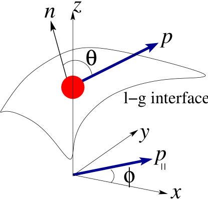
We start by deriving the equations of motion for an active Brownian particle that moves along a two-dimensional time-dependent surface profile $h(x,y,t)$, as shown schematically in Fig. 1. The three-dimensional position vector of the particle is given by ${\bm{r}}=(x,y,h(x,y,t))$. The kinematic equation for the velocity reads

$${\dot{\bm{r}}}=(\dot{x},\dot{y},\partial_{t}h+\dot{x}\partial_{x}h+\dot{y}\partial_{y}h).$$ (1)

Note that for fixed surface shape the velocity vector $\dot{\bm{r}}$ and the unit vector normal to the surface ${\bm{n}}=(-\partial_{x}h,-\partial_{y}h,1)/\sqrt{1+(\partial_{x}h)^{2}+(\partial_{y}h)^{2}}$ are orthogonal to each other: $\dot{\bm{r}}\cdot{\bm{n}}=0$.

In the overdamped limit the total velocity of the particle moving along the interface $h(x,y,t)$ is given by the superposition of the local tangential components of the self-propulsion velocity $v_{0}{\bm{p}}_{\tau}$, the local tangential fluid velocity ${\bm{u}}_{\tau}$ of the film, the tangential component of the gravity force ${\bm{g}}_{\tau}=-g({\bm{e}}_{z})_{\tau}$, and thermal noise ${\bm{\eta}}_{\tau}(t)$, which results in diffusion along the free surface,

$$\dot{{\bm{r}}}=v_{0}{\bm{p}}_{\tau}+{\bm{u}}_{\tau}+M\,m{\bm{g}}_{\tau}+{\bm{\eta}}_{\tau}(t)\,.$$ (2)

Here, $M$ denotes the mobility of the particle, $m$ its effective mass, which is reduced due to buoyancy effects for partly submerged particles, and the unit vector ${\bm{p}}$ indicates the direction of swimming. Thermal noise is characterized by a Gaussian random variable with zero mean and correlation function $\langle{\bm{\eta}}(t){\bm{\eta}}(t^{\prime})\rangle=2Mk_{B}T\delta(t-t^{\prime}){\bm{1}}_{2}$, where $k_{B}$ is the Boltzmann constant, $T$ is the absolute temperature, and ${\bm{1}}_{2}$ is a $2\times 2$ unit matrix. Note that the tangential component ${\bm{a}}_{\tau}$ of any vector ${\bm{a}}$ is given by

$${\bm{a}}_{\tau}={\bm{a}}-({\bm{a}}\cdot{\bm{n}}){\bm{n}}.$$ (3)

Furthermore, the fluid velocity ${\bm{u}}$ at the free surface satisfies the standard kinematic boundary condition resulting from continuity Oron et al. (1997)

$$\partial_{t}h=-u_{x}\partial_{x}h-u_{y}\partial_{y}h+u_{z}.$$ (4)

We consider particles swimming upward against gravity and pushing against the film surface. This already creates some polar order with a preferred vertical orientation of the swimmer bodies at the interface Enculescu and Stark (2011). Further reasons for such a polar order can be bottom-heaviness Wolff et al. (2013), the chemotactic response of bacteria swimming towards the surface in order to take up oxygen Dombrowski et al. (2004b), or any mechanism at the interface that aligns the particles along the vertical. In the following, we will not present a full derivation of the orientational distribution at the interface. Instead, for the distribution against the surface normal we will assume that it always adjusts instantaneously compared to the slow dynamics of the film interface (see below).

In what follows, we only take into account the long-wave deformations of the film surface, thus $\epsilon=h_{0}/\lambda\ll 1$, with $\lambda$ the wavelength of the surface deformations and $h_{0}$ the average film thickness. By noticing that the in-plane gradient $(\partial_{x},\partial_{y})$ is of order $\epsilon$, we obtain for the surface normal ${\bm{n}}=(0,0,1)+O(\epsilon)$ and for any vector ${\bm{a}}$ one has ${\bm{a}}_{\tau}=(a_{x},a_{y},0)+O(a_{z}\epsilon)+O(a_{x}\epsilon)+O(a_{y}\epsilon)$, as it follows from Eq. (3). Then, the Langevin equation (2) for the interfacial particle position becomes in leading order of $\epsilon$,

$$\dot{x} = v_{0}{\bm{p}}_{x}+{\bm{u}}_{x}+\eta_{x}(t),$$

$$\dot{y} = v_{0}{\bm{p}}_{y}+{\bm{u}}_{y}+\eta_{y}(t)\,.$$ (5)

Note that the tangential component of the gravity field vanishes in the long-wave limit, i.e. ${\bm{g}}_{\tau}=0$.

The instantaneous orientation of swimmers is indicated by the three-dimensional unit vector ${\bm{p}}$, as shown in Fig.1. For swimmers in the bulk of the fluid, the time-evolution of ${\bm{p}}$ is well known: it is determined by the rotation due to local fluid vorticity, alignment against some external field such as gravity, and random rotation with the rate controlled by the rotational diffusivity $D_{r}$. However, for swimmers at a free surface, the rate of change $\dot{\bm{p}}$ may be significantly modified as compared to bulk swimmers depending on the nature of the interaction between the swimmers and the free film surface. For instance, a surface swimmer only partly submerged in the fluid and possibly with elongated body shape is easily rotated by local fluid vorticity within the film surface. However, the rotational rate of ${\bm{p}}$ against the interface normal is possibly reduced as the interaction energies change with orientation of the swimmers at the free surface similar to anchoring effects for liquid crystals.

Here, we refrain from deriving the exact evolution equation for the orientation vector ${\bm{p}}$ of partly submerged surface swimmers. Instead, we use the argument from above to decouple the vertical component ${\bm{p}}_{\perp}$ from the in-plane component ${\bm{p}}_{\parallel}$. Thus, we assume that the evolution of the film surface is slow and the equilibration of ${\bm{p}}$ to a stationary distribution $P_{s}(\theta)$ with respect to the vertical is fast. In this case, the mean vertical component of ${\bm{p}}$ is given by

$$\langle{\bm{p}}_{\perp}\rangle=\int_{0}^{\pi}P_{s}(\theta)\cos{\theta}\,\sin{\theta}\,d\theta,$$ (6)

whereas the in-plane component ${\bm{p}}_{\parallel}$ can vary according to the in-plane dynamics of ${\bm{p}}$, which couples to the temporal film evolution. Note that $P_{s}(0)>P_{s}(\pi)$, which implies that the swimmers push on average against the liquid-gas interface.

As a result, the rotation of the in-plane component ${\bm{p}}_{\parallel}$ is described in terms of the polar angle $\phi$ (see Fig.1)

$$\dot{\phi}=\frac{1}{2}\Omega_{z}+\chi(t)\,,$$ (7)

where $\Omega_{z}=\partial_{x}u_{y}-\partial_{y}u_{x}$ is the vertical component of the local fluid vorticity and $\chi(t)$ is rotational noise with correlations $\langle\chi(t)\chi(t^{\prime})\rangle=2D_{r}\delta(t-t^{\prime})$. Furthermore, we introduce the mean in-plane velocity of an active particle, $v_{\parallel}=v_{0}[1-\langle{\bm{p}}_{\perp}\rangle^{2}]^{1/2}$ and substitute $v_{0}{\bm{p}}_{\parallel}$ in Eq. (II) by $v_{\parallel}{\bm{q}}=v_{\parallel}(\cos{\phi},\sin{\phi})$. Then, the Smoluchowski equation for the particle probability density $\rho(x,y,\phi,t)$, equivalent to Eqs. (II) and (7), reads

$$\partial_{t}\rho+{\bm{\nabla}}\cdot{\bm{J}}_{t}+\partial_{\phi}J_{r}=0,$$ (8)

where ${\bm{\nabla}}=(\partial_{x},\partial_{y})$ and the respective translational (${\bm{J}}_{t}$) and rotational ($J_{r}$) probability currents become Gardiner (2004); Pototsky and Stark (2012); Pototsky et al. (2014)

$${\bm{J}}_{t} = (v_{\parallel}{\bm{q}}+{\bm{u}}_{\parallel})\,\rho-Mk_{B}T({\bm{\nabla}}\rho),$$

$${J}_{r} = -D_{r}\partial_{\phi}\rho+\frac{1}{2}\Omega_{z}\rho.$$ (9)

The swimmers and the liquid-gas interface couple to each other through the local swimmer concentration $\rho(x,y,\phi,t)$ that acts twofold. First, each swimmer exerts the force $\alpha=v_{0}\langle p_{\perp}\rangle/M$ in the direction normal to the surface Alonso and Mikhailov (2009). So, the total pushing force $f_{n}$ of the swimmers per unit area is proportional to the direction-averaged local concentration of swimmers, $\langle\rho\rangle(x,y,t)=\int_{0}^{2\pi}\rho(x,y,\phi,t)\,d\phi$, and becomes

$$f_{n}(x,y,t)=\alpha\langle\rho\rangle(x,y,t)\,.$$ (10)

Secondly, the swimmers act as a surfactant and change the local surface tension. Assuming a relatively low concentration of swimmers, the surface tension $\sigma$ is known to decrease linearly with the local direction-averaged concentration $\langle\rho\rangle(x,y,t)$ Thiele et al. (2012),

$$\sigma=\sigma_{0}-\Gamma\langle\rho\rangle\,,$$ (11)

with the reference surface tension $\sigma_{0}$ and $\Gamma>0$.

Through Eqs. (10) and (11) the Smoluchowski equation (8) and the thin film equation in the long-wave approximation Oron et al. (1997) for the local film thickness $h(x,y,t)$ are coupled to each other Pototsky et al. (2014); Alonso and Mikhailov (2009),

$$\partial_{t}h+{\bm{\nabla}}\cdot\left(\frac{h^{3}}{3\mu}{\bm{\nabla}}\left[\sigma_{0}\Delta h-\rho_{l}gh+\alpha\langle\rho\rangle\right]\right)-\Gamma{\bm{\nabla}}\cdot\left(\frac{h^{2}}{2\mu}{\bm{\nabla}}\langle\rho\rangle\right)=0,$$ (12)

where $\rho_{l}$ is the density of the fluid and $\mu$ is its dynamic viscosity. The in-plane fluid velocity at the interface, ${\bm{u}}_{\parallel}=(u_{x},u_{y})$, is determined by the film profile $h(x,y,t)$ Oron et al. (1997),

$${\bm{u}}_{\parallel} = -\frac{\Gamma}{\mu}h{\bm{\nabla}}\langle\rho\rangle+\frac{h^{2}}{2\mu}{\bm{\nabla}}\left(\sigma_{0}\Delta h+\alpha\langle\rho\rangle\right),$$ (13)

and the vertical component of the vorticity is obtained as $\Omega_{z}=\partial_{x}u_{y}-\partial_{y}u_{x}$ from Eq. (13) not . Both, ${\bm{u}}_{\parallel}$ and $\Omega_{z}$ enter the currents (II) that determine the Smoluchowski equation (8). Note, that without swimming along the interface and rotational diffusion, one can integrate this equation over $\phi$ to recover the model in Ref. Alonso and Mikhailov (2009) with purely upwards pushing swimmers. Switching off the active swiming motion altogether one recovers the classical long-wave model for a dilute insoluble surfactant on a liquid film that may be written in a gradient dynamics form Thiele et al. (2012).

In what follows we focus on the instability induced by the pushing force generated by swimmers that swim predominantly upwards. To this end, we neglect the stabilising effect of the hydrostatic pressure $\rho_{l}gh_{0}$ as compared with the typical pushing force per unit area $\sim\rho_{0}v_{0}/M$. Experimentally, such a regime can be achieved by using, for example, bacteria-covered water films with a dense bacterial coverage. In the dilute limit treated in this manuscript, one needs conditions of microgravity. To illustrate this example, we present some estimates. The maximal self-propulsion force of a unicellular bacterium is known to be of the order of several $pN$ Stellamanns et al. (2014). The maximal surface density $\rho_{0}$ is estimated as $\rho_{0}\approx R^{-2}$, where $R\approx 1\mu$m is the typical size of the bacterial body. The dilute limit corresponds to densities of at least one order of magnitude below $R^{-2}$. Consequently, the maximal pushing force per unit are is estimated as $\rho_{0}v_{0}/M\approx 10^{-1}N/{\rm m}^{2}$. On the other hand, $\rho_{l}gh_{0}\approx g\,10^{-2}N/{\rm m}^{2}$ for a $10~{}\mu$m thick water film. Clearly, $\rho_{l}gh_{0}$ can be neglected against $\rho_{0}v_{0}/M$ in case of $g\ll 10\,{\rm m}/s^{2}$.

The possibility to experimentally detect the thin-film instability due to the pushing force $\alpha$ exerted by self-phoretic particles is further strengthened by recent experiments with $\sim 30$ nm small Janus particles Lee et al. (2014). A much smaller particle size allows for larger surface particle densities and may give rise to larger excess pressure. In fact, the maximal density increases as $\sim R^{-2}$ for decreasing particle size $R$. However, it remains unclear how the pushing force $\alpha$ of a single self-phoretic particle scales with its size. If the decrease of the pushing force with $R$ is slower than $\sim R^{2}$, the resulting excess pressure $\sim\rho_{0}f$ exerted by the particles onto the liquid-gas interface can be several orders of magnitude larger than the value of $\approx 10^{-1}N/{\rm m}^{2}$ estimated before in the dilute limit of a bacterial carpet.

For all what follows, we non-dimensionalise the evolution equations for film thickness $h(x,y,t)$ and swimmer density $\rho(x,y,\phi,t)$ employing the scaling as in Ref. Pototsky et al. (2014). Thus, we use $h_{0}$ as the vertical length scale, $h_{0}\sqrt{\sigma_{0}/\Gamma\rho_{0}}$ as the horizontal length scale, $\mu h_{0}\sigma_{0}/(\Gamma^{2}\rho_{0}^{2})$ as the time scale, and the direction-averaged density of swimmers in the homogeneous state $\rho_{0}$ as the density scale. This gives the relevant parameters of our model: the dimensionless in-plane self-propulsion velocity $V=v_{\parallel}\mu\sigma_{0}^{1/2}/(\Gamma\rho_{0})^{3/2}$, the dimensionless in-plane rotational diffusivity $D=D_{r}h_{0}\mu\sigma_{0}/(\Gamma\rho_{0})^{2}$, the translational surface diffusivity $d=k_{B}TM\mu/(h_{0}\rho_{0}\Gamma)$, and the excess pressure parameter $\beta=\alpha h_{0}/\Gamma$. Furthermore, we introduce the effective in-plane diffusivity

$$D_{\rm eff}=\frac{V^{2}}{2D}+d\,.$$ (14)

Note that $D_{\rm eff}$ corresponds to the diffusion coefficient of a single self-propelled Brownian particle moving along a flat two-dimensional surface Palacci et al. (2010b); ten Hagen et al. (2011). In Appendix VI we summarize our non-dimensionalised dynamic equations.

III Linear stability of a flat film with homogeneously distributed swimmers

III.1 General

We start by presenting more details of our stability analysis of the flat film as compared to our previous work Pototsky et al. (2014) including an analytical treatment and a more thorough discussion of the occuring dispersion relations. We linearise the non-dimensionalized Eqs. (8) and (12) about the homogeneous isotropic steady state given by $h=1$, $\rho=1$, using the ansatz

$$h(x,y,t)=1+\delta h,~{}~{}\rho(x,y,\phi,t)=1+\delta\rho,$$ (15)

where $\delta\rho,\delta h\ll 1$. The linearised Smoluchowski equation (8) and the thin film equation (12) become, respectively,

$$\partial_{t}\delta\rho+{\bm{\nabla}}\cdot\left(V{\bm{q}}\delta\rho\right)+\Delta\left[\left(\frac{1}{2}\beta-1\right)\langle\delta\rho\rangle+\frac{1}{2}\Delta(\delta h)\right]\frac{1}{2\pi}-d\Delta\delta\rho-D\partial^{2}_{\phi}\delta\rho=0.$$ (16)

$$\partial_{t}(\delta h)+\frac{1}{3}\left[\Delta^{2}(\delta h)+\beta\Delta\langle\delta\rho\rangle\right]-\frac{1}{2}\Delta\langle\delta\rho\rangle=0,$$ (17)

with $\langle\delta\rho\rangle=\int_{0}^{2\pi}\delta\rho(x,y,\phi,t)\,d\phi$. The linearised surface velocity $(\delta u_{x},\delta u_{y})$ from Eq. (13) reads

$$\delta{\bm{u}}_{\parallel}=-{\bm{\nabla}}\langle\delta\rho\rangle+\frac{1}{2}{\bm{\nabla}}\left[\Delta(\delta h)+\beta\langle\delta\rho\rangle\right]\,.$$ (18)

Next, we follow Pototsky et al. (2014) and Fourier transform the perturbations $\delta h$ and $\delta\rho$ by using a continuous Fourier transform in space and a discrete Fourier transform in the angle $\phi$. Combining this with an exponential ansatz for the time evolution of the individual modes we have

$$\delta h({\bm{r}},t) = \int\hat{h}({\bm{k}})e^{\gamma({\bm{k}})t}e^{I{\bm{k}}{\bm{r}}}\,d{\bm{k}},$$

$$\delta\rho({\bm{r}},\phi,t) = \lim_{N\rightarrow\infty}\frac{1}{2\pi}\sum_{n=-N}^{N}e^{In\phi}\int W_{n}({\bm{k}})e^{\gamma({\bm{k}})t}e^{I{\bm{k}}{\bm{r}}}\,d{\bm{k}},$$ (19)

with the small dimensionless Fourier amplitudes $\hat{h}({\bm{k}})$ and $W_{n}({\bm{k}})$, the wave vector of the perturbation ${\bm{k}}=(k_{x},k_{y})$, and the real or complex growth rate $\gamma({\bm{k}})$. Substituting the expansions from Eqs. (III.1) into the linearized Eqs. (8,12), we obtain the eigenvalue problem

$$\gamma({\bm{k}})\mathbf{H}={\mathcal{J}}({\bm{k}})\mathbf{H},$$ (20)

with the eigenvector $\mathbf{H}$

$${\mathbf{H}}({\bm{k}})=(\hat{h},W_{0},W_{1},W_{-1},W_{2},W_{-2},\dots),$$ (21)

and the Jacobi matrix $\mathcal{J}$, which corresponds to a banded matrix of the structure

$$-{\mathcal{J}}({\bm{k}})=\left(\begin{array}[]{ll|llllll}T_{11},&T_{12},&0&0&0&0&0&\dots\\ T_{21},&T_{22},&V^{(-)},&V^{(+)},&0&0&0&\dots\\ \hline\cr 0&V^{(+)},&D+dk^{2},&0&V^{(-)},&0,&0&\dots\\ 0&V^{(-)},&0&D+dk^{2},&0&V^{(+)},&0&\dots\\ 0&0&V^{(+)},&0&2^{2}D+dk^{2},&0&V^{(-)}&\dots\\ 0&0&0&V^{(-)},&0&2^{2}D+dk^{2},&0&\dots\\ 0&0&0&0&V^{(+)},&0&3^{2}D+dk^{2}&\dots\\ \dots\end{array}\right),$$ (30)

where $k^{2}=k_{x}^{2}+k_{y}^{2}$, $V^{(+)}=\frac{Vk_{y}}{2}+\frac{iVk_{x}}{2}$, $V^{(-)}=-\frac{Vk_{y}}{2}+\frac{iVk_{x}}{2}$. The $(2\times 2)$ matrix ${\bm{T}}$ in the upper left corner of $\mathcal{J}$ is given by

$${\bm{T}}({\bm{k}})=\left(\begin{array}[]{ll}\frac{1}{3}k^{4},&\left(\frac{1}{2}-\frac{\beta}{3}\right)k^{2}\\ \frac{1}{2}k^{4},&\left(1-\frac{1}{2}+d\right)k^{2}\end{array}\right).$$ (33)

Note that the matrix ${\bm{T}}$ coincides with the Jacobi matrix derived in Ref. Alonso and Mikhailov (2009) that encodes the linear stability in the special case of a flat film covered by autonomous purely upwards pushing motors that exert an excess pressure onto the liquid-gas interface. In practice, we truncate the expansion in the angle $\phi$ and only take the first $N$ Fourier modes into account. Then, the Jacobi matrix $\mathcal{J}$ is a $(2N+2)\times(2N+2)$ matrix and the truncated eigenvector $\mathcal{H}=(\hat{h},W_{0},W_{1},W_{-1},\dots,W_{N},W_{-N})$ is $(2N+2)$ dimensional.

Figure 2: (Color online) (a) Stability diagram of a flat film with homogeneous distribution of particles for $\beta=4$ and $d=0.05$. In the stable lightly-shaded region Re$[\gamma(k)]<0$ for all values of the wave number $k$. The finite wave number instability sets in along the line marked by “fw”. The zero wave number instability sets in along the vertical dashed line $D_{\rm eff}=1$, marked by “zw”. The inset zooms into the region marked by the rectangle in the main panel: In the strongly shaded area marked “MI”, the mixed type fw /zw instability occurs. Panels (b-d) show Re$[\gamma(k)]$ of the two leading eigenvalues for parameters taken (b) at point $1$ ($V=3.5$, $D=10$, i.e., $D_{\rm eff}=0.66$), (c) at point $2$ ($V=3.5$, $D=1$, i.e., $D_{\rm eff}=6.175$), and (d) at point $3$ ($V=2$, $D=2.4$, i.e., $D_{\rm eff}=0.88$) in panel (a). Dashed and solid lines indicate complex and real eigenvalues, respectively. The inset in (d) zooms into the region marked by the rectangle.

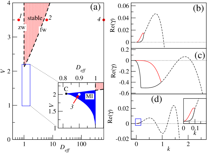
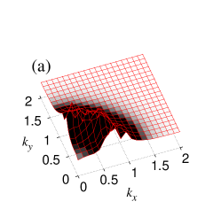
The stability diagram of the homogeneous isotropic state, as computed for reduced excess pressure $\beta=4$ and translational diffusivity $d=0.05$ from Eqs. (20) is shown in Fig. 1(a) in the parameter plane spanned by the reduced in-plane velocity $V$ and the effective diffusion constant $D_{\rm eff}=V^{2}/(2D)+d$ of the surfactants. We numerically compute the eigenvalues of the truncated Jacobi matrix Eqs. (30) for $N=10$ Fourier modes and then check the results by doubling the number of the Fourier modes to $N=20$. Note that the choice $\beta=4$ and $d=0.05$ corresponds to a flat film that is unstable at zero in-plane velocity, $V=0$ as $\beta>\beta_{c}(d)=2(1+d)$, the critical value for the onset of the long-wave instability Alonso and Mikhailov (2009), e.g., $\beta_{c}=2.1$ for $d=0.05$. In what follows, we characterize the system by the set of parameters $(V,D)$ and also indicate the respective value of $D_{\rm eff}$.

For the system with non-zero in-plane velocity ($V\not=0$), we have earlier reported the existence of two different instability modes Pototsky et al. (2014). Namely, for sufficiently large $V$, there exists a wedge-shaped stability region, marked in Fig.2(a) by “stable” that separates regions where the two different instability modes occur. The wedge opens at $V_{c}\approx 2.05$ towards larger values of $V$, i.e., at any $V>V_{c}$, there exists a window in the effective diffusivity $D_{\rm eff}$ for which the flat homogeneously covered film is stable (note that $V_{c}$ depends on $\beta$ and $d$).

By crossing the two borders of the linearly stable region, the system changes stability via two distinct instability modes. The first mode corresponds to an oscillatory instability with a finite wave number at onset, i.e., a travelling wave instability. In this case, for parameters directly on the stability threshold, the leading eigenvalue $\gamma(k)$ of the Jacobi matrix from Eq. (30) has a negative real part for all values of the wave number $k$, except for the critical wave number $k_{c}\not=0$, where $\gamma(k)$ has the form $\gamma(k_{c})=\pm iW_{c}$ with some non-zero frequency $W_{c}$. We will refer to this instability mode as the finite wave number instability (fw). The second mode ($zw$) corresponds to an instability with a zero wave number at onset. This mode is characterized in detail in the next section.

III.2 Zero wave number instability: analytic results

In the following we present an approximate analytic expression for the zero wave number instability. We start by introducing the Fourier transformed fields $\hat{\delta h}({\bm{k}},t)$ and $\hat{\rho}({\bm{k}},\phi,t)$, according to $\delta h({\bm{r}})=\int e^{i{\bm{k}}\cdot{\bm{r}}}\hat{\delta h}({\bm{k}},t)\,d{\bm{k}}$ and $\rho(\bm{r})=\int e^{i{\bm{k}}\cdot{\bm{r}}}\hat{\rho}({\bm{k}},\phi,t)\,d{\bm{k}}$, into Eq. (16) and obtain

$$\partial_{t}\hat{\rho}+V\left(ik_{x}\cos{\phi},ik_{y}\sin{\phi}\right)\hat{\rho}+\frac{1}{2\pi}\left(1-\frac{\beta}{2}\right)k^{2}\hat{\langle\rho\rangle}+\frac{1}{4\pi}k^{4}(\hat{\delta h})+d\,k^{2}\hat{\rho}-D\partial^{2}_{\phi}\hat{\rho}=0.$$ (34)

Close to the threshold of the zero wave number instability, the amplitudes of all modes with the wave number $k\not=0$ rapidly decay with time. Therefore, in the limit $k\rightarrow 0$, in Eq. (34) one may neglect the terms of orders $k^{2}$ and $k^{4}$ as compared to the ones of order $k^{0}$ and $k$. In consequence, the density and film height equations decouple. In fact, to this order the density equation describes a single self-propelled particle with rotational diffusivity $D$ and self-propulsion velocity $V$ but with neglected translational diffusivity.

To proceed further, we note that on length scales larger than the persistence length of an active particle, $V/D$, the dynamics becomes purely diffusive. To arrive at this result, one performs a multipole expansion of $\hat{\rho}({\bm{k}},\phi,t)$ in the angle $\phi$ using only the monopol $\hat{\langle\rho\rangle}$ and the dipole moment Golestanian (2012); Pohl14 . The latter can be elimated in the dynamic equation for $\hat{\langle\rho\rangle}$ and from Eq. (34) one arrives at

$$\partial_{t}\hat{\langle\rho\rangle}+\left(1-\frac{\beta}{2}+D_{\rm eff}\right)k^{2}\hat{\langle\rho\rangle}+\frac{1}{2}k^{4}\hat{\delta h}=0,$$ (35)

which is coupled to the linearised thin film equation in Fourier space

$$\partial_{t}(\hat{\delta h})+\frac{1}{3}\left[k^{4}\hat{\delta h}-\beta k^{2}\hat{\langle\rho\rangle}\right]+\frac{1}{2}k^{2}\hat{\langle\rho\rangle}=0.$$ (36)

Here, $D_{\rm eff}=V^{2}/(2D)+d$ is the effective diffusion constant of an active particle introduced earlier in Eq. (14). The additional term results from the activity of the particle. Equations (35) and (36) are identical to the linearised evolution equations found for the concentration field of the purely upwards swimming ($V=0$) surfactant particles coupled to the thin film equation, as studied in Ref.Alonso and Mikhailov (2009). In fact, the results of the linear stability analysis of Ref. Alonso and Mikhailov (2009) can be translated to the system of equations (35) and (36) by setting the translational diffusivity of the purely upwards swimming particles to be equal to $D_{\rm eff}$.

The two eigenvalues $\gamma(k)$ resulting when introducing an exponential ansatz for the time dependence into Eqs. (35) and (36) are determined analytically (cf. Ref. Alonso and Mikhailov (2009)). The Jacobi matrix ${\bm{J}}(k)$ of the linearised Eqs. (35) and (36) is given by

$${\bm{J}}=-k^{2}\,\left(\begin{array}[]{cc}\frac{k^{2}}{3}&\frac{1}{2}-\frac{\beta}{3}\\ \frac{k^{2}}{2}&\eta\end{array}\right),$$ (39)

where we introduced $\eta=1-\beta/2+D_{\rm eff}$. The two eigenvalues $\gamma_{1,2}$ are

$$\gamma_{1,2}=\frac{1}{2}\left({\rm tr}({\bm{J}})\pm\sqrt{{\rm tr}({\bm{J}})^{2}-4{\rm det}({\bm{J}})}\right),$$ (40)

with ${\rm tr}({\bm{J}})=-k^{2}[k^{2}/3+\eta]$ and ${\rm det}({\bm{J}})=k^{6}(1/12+D_{\rm eff}/3)$.

Figure 3: (Color online) Comparison of the numerically computed two leading eigenvalues (solid and dashed lines represent real and complex eigenvalues, respectively) and the analytic prediction of Eq. (40) (dotted lines). (a) $V=3.5$, $D_{\rm eff}=0.66$, (b) $V=2$, $D_{\rm eff}=0.88$. The inset zooms into the region marked by the rectangle, where the analytic and numerical results are indistinguishable from each other. In the inset we only show the analytically computed eigenvalues.

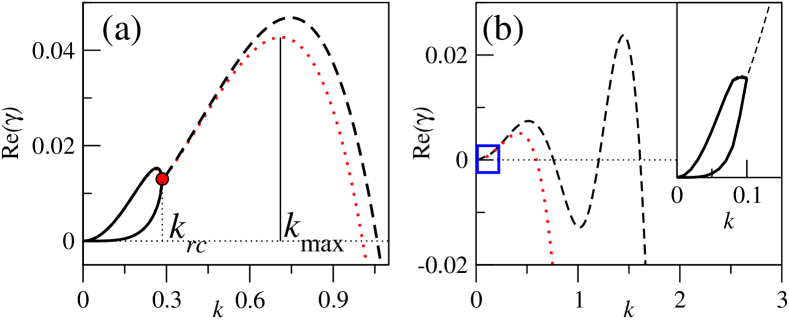
In Fig. 3(a,b) we compare the analytic eigenvalues given by Eq. (40) with the two leading eigenvalues of the original non-reduced system, computed numerically, as described in Section III.1. Solid and dashed lines correspond to the numerically computed real and complex eigenvalues, respectively, dotted lines correspond to Eq. (40). Fig. 3(a) is obtained for the parameters corresponding to point $1$ in Fig. 2(a), i.e., $V=3.5$ and $D_{\rm eff}=0.66$, and Fig. 3(b) corresponds to point $3$ in Fig. 2(b), i.e., $V=2$ and $D_{\rm eff}=0.88$. In both cases, the agreement is excellent up to $k\approx 0.4$.

Next, we use Eq. (40) in order to classify the zero wave number instability that sets in along the dashed vertical line marked by “zw” in Fig. 2(a). Analysing the eigenvalues in Eq. (40) shows that the real part of the leading eigenvalue changes its sign at $\eta=0$, or, equivalently at $D_{\rm eff}=\beta/2-1$. Thus, for the value of $\beta=4$ used here, we obtain $D_{\rm eff}=1$, in agreement with Fig.2(a). We emphasize that the above analytic results can only be applied in the limit of $k\ll 1$, where the approximation (35) applies.

We find that in the unstable region, i.e., for $\eta<0$, the fastest growing wave number $k_{\rm max}$, indicated in Fig. 3(a), always corresponds to a pair of two complex conjugate eigenvalues [dashed line in Fig. 3(a)]. By locating the maximum of ${\rm tr}[J(k)]$, we determine $k_{\rm max}$ and its complex growth rate,

$$k_{\rm max}=\sqrt{\frac{3}{2}\mid\eta\mid},\,\,\,{\rm Re}[\gamma(k_{\rm max})]=\frac{3}{8}\eta^{2},\,\,\,{\rm Im}[\gamma(k_{\rm max})]=\pm\frac{\mid\eta\mid}{2}\sqrt{\frac{27}{2}\mid\eta\mid\left(\frac{1}{12}+\frac{D_{\rm eff}}{3}\right)-\frac{9}{16}\eta^{2}}.$$ (41)

For $k<k_{\rm rc}<k_{\rm max}$, the two leading eigenvalues are real, as indicated by the two solid lines in Fig. 3(a). The wave number $k_{\rm rc}$ is

$$k_{\mathrm{rc}}=\sqrt{\frac{3\eta^{2}}{1+4D_{\rm eff}-2\eta}}\approx\sqrt{\frac{3}{1+4D_{\rm eff}}}\mid\eta\mid.$$ (42)

This result implies that the character of the zero wave number instability is peculiar: Directly at onset ($\eta=0$) the leading two eigenvalues are real, however, already arbitrarily close above onset ($\eta<0$) the band of unstable wavenumbers contains a region of real modes (close to and including $k=0$) and a region of complex modes (always including the fastest growing mode). This behaviour is related to the existence of two conserved fields, $h$ and $<\rho>$, that forces two real modes with growh rate zero at $k=0$. In consequence, the fastest growing wave number $k_{\rm max}$ tends to zero when approaching the stability threshold from above. Here, we call this scenario a zero-wave number instability.

III.3 Mixed instability

The analytic results obtained in the previous section give for the zero wave number instability the threshold $D_{\rm eff}=1$ for $\beta=4$. This perfectly coincides with the numerically computed threshold as indicated by the left thick dashed line in Fig.2(a). However, these results also remain valid around $D_{\rm eff}=1$ for small values of $V<V_{c}$ deep in the unstable region. This implies that regardless of the value of $V$, the sign of the dispersion curve ${\rm Re}[\gamma(k)]$ at very small wave numbers $k\approx 0$ changes from negative to positive as $D_{\rm eff}$ is decreased past the critical value $D_{\rm eff}=1$ (at $\beta=4$). However, there will always be an instability at a non-zero wave number, as we explain now.

We observe a mixed-instability region, marked by ”MI” and heavily shaded in the inset of Fig. 2(a), where the system can be described as being unstable with respect to a mixed finite- and zero-wavelength instability. In this region, there exist two bands of unstable wave numbers: one with $k\in[0,k_{1}]$ and another one with $k\in[k_{2},k_{3}]$, with $k_{3}>k_{2}>k_{1}>0$. The two leading eigenvalues that correspond to the pure zero wave number, the pure finite wave number, and the mixed instabilities, are shown in Figs. 2(b), (c), and (d), respectively. The respective parameters are; point 1: $V=3.5,\,D=10$, i.e., $D_{\rm eff}=0.66$, point 2: $V=3.5,\,D=1$, i.e., $D_{\rm eff}=6.175$ in the main panel, and point 3: $V=2,\,D=2.4$, i.e. $D_{\rm eff}=0.88$ in the inset of Fig. 2(a). Dashed and solid lines correspond, respectively, to complex and real eigenvalues.

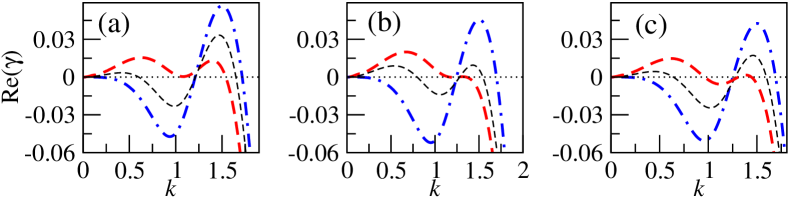
When considering the type of dispersion curves, the transition from the finite wave number instability to the zero wave number instability can follow two different scenarios. We identify them by keeping $V$ constant and gradually decrease $D_{\rm eff}$. In the first scenario for $V\gtrsim V_{c}=2.05$, the maximum of ${\rm Re}[\gamma((k)]$ in Fig. 2(c) first becomes negative, i.e., the finite wave number instability is stabilised while crossing the ”fw” line in the stability diagram. Subsequently, the system crosses the ”zw” line and becomes unstable w.r.t. the zero wave number mode. In the second scenario for $V\lesssim V_{c}=2.05$, the system first crosses the line $D_{\rm eff}=1$ and enters the mixed instability region. Then the dispersion curve as in Fig. 2(d) gradually transforms into the dispersion curve of the zero wave number instability, while leaving the region MI. We also remark that the mixed instability region stretches from $V=V_{c}$ down $V=0$. However, its horizontal width is negligibly small for $V<1$.

The second scenario is visualised in Fig. 4. In Fig. 4(a) we fix $V=2$ and plot ${\rm Re}[\gamma((k)]$ for three different $D_{\rm eff}$: $D_{\rm eff}=1$ (thick dotted-dashed blue line), $D_{\rm eff}=0.92$ (dashed black line) and $D_{\rm eff}=0.83$ (thick dashed red line). In this case, the transition from the mixed instability to the zero wave number instability occurs through the elevation of the local minimum of the dispersion curve, so that a single band of unstable wave numbers occurs starting at $k=0$.

In Fig. 4(b) we fix $V=2.0275$ what corresponds to the level of the cusp point marked by ”C” in the inset of Fig. 2(a). We show ${\rm Re}[\gamma((k)]$ for $D_{\rm eff}=1$ (thick dotted-dashed blue line), $D_{\rm eff}=0.87$ (dashed black line) and $D_{\rm eff}=0.81$ (thick dashed red line). In this case, the transition from the mixed instability to the zero wave number instability occurs through the simultaneous elevation of the local minimum and the depression of the local maximum of the dispersion curve. In Fig.4(c) we fix $V=2.03$ and plot ${\rm Re}[\gamma((k)]$ for $D_{\rm eff}=1$ (thick dotted-dashed blue line), $D_{\rm eff}=0.9$ (dashed black line) and $D_{\rm eff}=0.84$ (thick dashed red line). In this case, the transition from the mixed instability to the zero wave number instability occurs through the depression of the local maximum of the dispersion curve. All dispersion curves in Fig. 4 correspond to real eigenvalues only for a very narrow band of the wave numbers $k\approx 0$ (details are not shown here).

Figure 4: (Color online) Transition from the finite wave number to the zero wave number instability region while passing through the mixed instability at fixed $V$ by increasing $D$ (decreasing $D_{\rm eff}$). In each panel $V$ is fixed and three different values of $D$ are chosen. The thick dotted-dashed (blue) lines correspond to $D_{\rm eff}=1$, the thick dashed (red) lines represent the critical dispersion curve on the border of the MI region in Fig. 2 at $D_{\rm eff}<1$, and the thin dashed (black) line is for a value of $D_{\rm eff}$ in between. The transitions are shown along the lines: (a) $V=2$, (b) $V=2.0275$ corresponding to the cusp point C in the inset of Fig.2(a)], and (c) $V=2.03$.

IV Nonlinear evolution

IV.1 Numerical approach and solution measures

In this section we address the system of nonlinear evolution equations for film hight $h$ and probability density $\rho$, which we give in non-dimensional form in Eqs. (VI) and (50) in appendix VI. In order to solve them numerically, we discretize both the film thickness $h(x,y,t)$ and the density $\rho(x,y,\phi,t)$ in a square box for the spatial coordinates with $(x\in[-L/2,L/2])\times(y\in[-L/2,L/2])$ and in the interval $\phi\in[0,2\pi]$ for the orientation angle always using periodic boundaries. We use $N=100$ or $N=128$ mesh points for each spatial direction to discretise space and $20$ Fourier modes for the decomposition of the $\phi$-dependence of the density. We adopt a semi-implicit pseudo-spectral method for the time integration, as outlined in the Appendix and verify some of our results by using a fully explicit Euler scheme with the time step of the order of $\Delta t=10^{-4}\dots 10^{-5}$.

In order to quantify the spatio-temporal patterns in film hight and density, we introduce three global measures: the mode type $M$ with

$$M=L^{-2}\int\int(h(x,y,t)-1)(\langle\rho\rangle(x,y,t)-1)\,dxdy,$$ (43)

characterizes if spatial modulations of the film surface $h(x,y,t)$ and the average density $\langle\rho\rangle(x,y,t)$ are predominantly in-phase ($M>0$) or predominantly in anti-phase ($M<0$); the space-averaged flux of the fluid $\bar{\bm{J}}_{h}$ determined by

$$\bar{\bm{J}}_{h} = L^{-2}\int\int\left(\frac{h^{3}}{3}{\bm{\nabla}}\left[\Delta h+\beta\langle\rho\rangle\right]-\frac{1}{2}\left(h^{2}{\bm{\nabla}\langle\rho\rangle}\right)\right)\,dxdy$$ (44)

allows us to distinguish between standing waves that correspond to $\bar{\bm{J}}_{h}=0$ and travelling or modulated waves that are characterized by a non-zero fluid flux; and finally the space-averaged translational flux of the swimmers,

$$\bar{\bm{J}}_{t} = L^{-2}\int\int\left(V\langle\rho{\bm{q}}\rangle+{\bm{U}}_{\parallel}\langle\rho\rangle\right)\,dxdy,$$ (45)

indicates global surface motion of the swimmers.

In the following we indicate the richness in the dynamics of our system by giving examples of evolving patterns for specific parameter sets located in the stability diagram of Fig. 2(a). Mapping out a full state diagram is beyond the scope of this article.

IV.2 Regular standing wave pattern

We first study the parameters $V=3.5$ and $D=1$ ($D_{\rm eff}=6.175$) in the unstable region of the phase diagram Fig. 2(a), close to the finite wave number instability threshold [point $2$ in Fig. 2(a)]. The corresponding dispersion curve is shown in Fig. 2(c). The system size $L=20$ is set to be several times larger than the fastest growing wave length equal to $2\pi/k_{\rm max}=3.43$, with $k_{\rm max}$ denoting the wave number corresponding to the maximum of the dispersion curve. By numerically integrating Eqs. (VI), we study the temporal evolution of the system from the homogeneous isotropic steady state $h=1$ and $\rho=1/(2\pi)$, i.e., the trivial state. The initial conditions are given by $h=1+\delta h(x,y)$ and $\rho=1/(2\pi)+\delta\rho(x,y,\phi)$, where the small amplitude random perturbations $\delta h(x,y)$ and $\delta\rho(x,y,\phi)$ represent two independent sources of white noise.

Figure 5: (Color online) Standing wave pattern, obtained for $V=3.5$, $D=1$, $d=0.05$, i.e., $D_{\rm eff}=6.175$ [the corresponding dispersion curve is shown in Fig. 2(c)]. The snapshots are taken at $t=190$: (a) average density $\langle\rho\rangle(x,y)$ (grey scale map) with average orientation field (red arrows) and (b) the film thickness $h(x,y)$. $\Psi$ is the angle between the main lattice direction and the horizontal axis. Plotted versus time are: (c) The mode type $M$ from Eq. (43), (d) zoom of the region in (c) marked by the red rectangle, and (e) local film thickness $h(t)$ at a randomly chosen point on the surface.

Figure 6: (Color online) Standing stripe patterns with periodically changing directions for the same parameters as in Fig. 5. Shown is a small portion of the square domain in Fig. 5 over one oscillation cycle with period $T=1.15$. Five snapshots of the film thickness $h(x,y,t)$ (in grey scale map) are plotted together with a contour plot of the average density $\langle\rho\rangle$ at the level of $\langle\rho\rangle=1$. Arrows indicated the shift vector of the pattern during the four phases of one oscillation cycle.

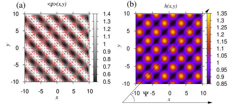
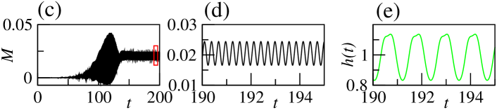
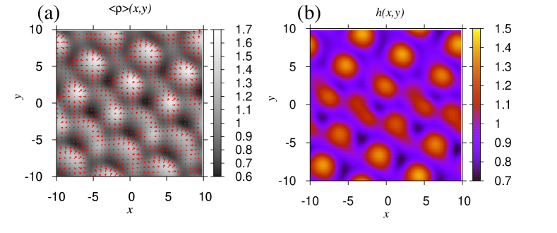
We found that after a transient phase of an approximate duration of $100\dots 200$ time units, the system settles onto a stable time-periodic state. It can be characterised as a regular standing wave, where stripe patterns change periodically between the two diagonal directions as Movie 1 shows. The mean fluid flux is zero, $\bar{J}_{h}=0$. Figure. 5(a) shows a snapshot of the average density $\langle\rho\rangle(x,y)$ in grey scale map together with the average orientation field $\langle{\bm{q}}\rangle=(\langle\cos{\phi}\rangle,\langle\sin{\phi}\rangle)$ shown by red arrows at time $t=190$. The corresponding snapshot of the film thickness $h(x,y)$ is shown in Fig. 5(b). The patterns in Figs. 5(a) and (b) are highly dynamic, with the shape of the surfaces $h$ and $\langle\rho\rangle$ changing periodically in time, visualized in Movie 1 and described in Fig.6. Fig. 5(b) indicates the moment in time when the orientiation of the stripes in the film profile changes from one diagonal to the other. Maxima in the film height $h(x,y,t)$ occur, which are arranged in a perfect square lattice, tilted by the angle $\Psi\approx\pi/4$ w.r.t. the $x$-axis.

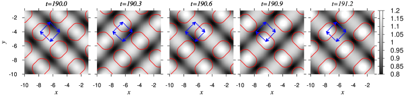
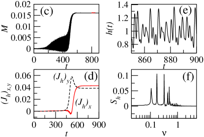
The time evolution of the mode type $M$ starting from the initially homogeneous state is plotted in Fig. 5(c). After $150$ time units $M$ starts to oscillate periodically about the average of $\overline{M}=0.02$, as indicated in Fig. 5(d), where the zoom of the region marked by the rectangle in Fig. 5(c) is shown. As $M>0$, the oscillations of the film thickness and the averaged density are in-phase. The temporal period $T$ of the standing wave can be determined by observing the oscillations of the film thickness $h(t)$ at a randomly chosen point, as Fig. 5(e) demonstrates. Thus $h(t)$ oscillates about the average film thickness $h=1$ as a perfect periodic function with the period $T=1.15$.

Remarkably, the temporal oscillations of $M$ in Fig. 5(d) are four times faster than the oscillations in film thickness. This is due to the fact that a complete period of the standing wave consists of four phases, where the same spatial pattern reappears four times, each time shifted along one side of a square and rotated by $90^{\circ}$. Because $M$ is invariant under rotation and translation of the pattern, the oscillation period of $M$ is four times smaller then the overall period of the standing wave. The four shifted and rotated patterns are clearly seen in Movie 1 when concentrating on the cubic lattice formed by the maxima in the height profile. In Fig. 6 we illustrate the four phases by snapshots of the transient stripe patterns. During the first phase, the maxima of the average density $\langle\rho\rangle$ shift along a straight line by a distance $l_{w}/2$ equal to half the spatial period $l_{w}$. The maxima of the film thickness follow the same path. In each subsequent phase, the shift occurs along the direction that is orthogonal to the previous shift. After completing all four phases, the maxima of $\langle\rho\rangle$ and also of $h$ will have traveled along the sides of a square with the side length $l_{w}/2$ and have returned to the initial position. In between the square patterns, formed by the maxima in density, the film thickness assumes patterns of parallel ridges that during each quarter of the cycle decay into the square pattern, formed by the maxima in $h$, and reappear rotated by $\pi/2$. One may say that during one cycle the pattern oscillates through several accessible patterns that are well known solutions for pattern forming systems on a square. In particular, they are known to occur as (stable or unstable) steady states in thin film equations that describe ’passive’ liquid layers, ridges and drops on homogeneous solid substrates Beltrame and Thiele (2010).

The spatial period of the standing wave, $l_{w}$, can be determined in real space by measuring the distance between two nearest maxima (minima) of the height profile $h(x,y)$ taken at an arbitrary moment of time. The maximal error in this procedure is of the order of $\sqrt{2}L/N$ where $N$ is the number of discretization points along the $x$ and $y$ axis and the factor $\sqrt{2}$ reflects that the wave is directed along the diagonal of the domain. We obtain $l_{w}=3.5\pm 0.14$ for the square patterns in Fig. 5 using $L=20$ and $N=100$ to estimate the error.

Due to the periodic boundary conditions the measured $l_{w}$ of the patterns in Fig. 5 is slightly different from the fastest growing wave length found from the dispersion curve in Fig. 2(b) as $l_{\mathrm{max}}=2\pi/k_{\mathrm{max}}=3.43$. This difference is explained as follows. In order to fulfill periodic boundary conditions in a square domain of size $L$, the periods of a wave projected, respectively, on the $x$ and $y$ axis are $L/k$ and $L/m$, where $m$ and $k$ are some integers. This restricts the possible rotation angles $\Psi$ of a periodic pattern relative to the $x$ axis (see Fig. 5). They have to satisfy

$$\cos{\Psi}=\frac{m}{\sqrt{k^{2}+m^{2}}},\,\,\,\sin{\Psi}=\frac{k}{\sqrt{k^{2}+m^{2}}}$$ (46)

and the wave length of the pattern becomes $l_{w}=L/\sqrt{k^{2}+m^{2}}$. Thus, for the parameters used in Fig. 5, the random initial conditions select the possible rotation angle $\Psi=\pi/4$. This choice corresponds to $m=k$ in Eq. (46). Next, the integer $m=4$ is chosen in such a way that the resulting wave length of the pattern, $l_{w}=L/(m\sqrt{2})=3.53$, is close to the fastest growing wave length of $l_{\mathrm{max}}=3.43$.

For later use, we mention that the spatial period $l_{w}$ and the angle $\Psi$ of a simulated periodic pattern can be determined by computing the time-averaged power spectral density of the film thickness profile $h(x,y,t)$ according to

$$S_{h}({\bm{k}})=\frac{1}{T}\int_{t}^{t+T}|\hat{h}({\bm{k}})|^{2}\,dt,$$ (47)

where $T$ is the temporal period of oscillations and $\hat{h}({\bm{k}})$ denotes the discrete Fourier transform of $h(x,y,t)$. The periodic boundary conditions for the square domain only allow for a discrete set of possible wave vectors forming a square lattice with lattice constant $\Delta k=2\pi/L\approx 0.31$. Any periodic pattern in the height modulation $h(x,y)$ gives a major peak of the power spectrum in Eq. (47), which is located at $k_{x}=2\pi m/L$, $k_{y}=2\pi k/L$, with the same integers $m$ and $k$ as in Eq. (46). Depending on the shape of the surface, secondary peaks (higher harmonics) might be present, but their strengths are typically orders of magnitude smaller compared to the major peak.

In systems of active matter, stable square patterns have previously been found in Vicsek-type models with memory. It was shown that in the case of a ferromagnetic alignment between the self-propelled particles with memory in the orientational ordering the system settles to a perfectly symmetric state with a checkerboard arrangement of clockwise and anti-clockwise vortices Nagai et al. (2015). Using our classification, this checkerboard lattice corresponds to a square pattern with the main axis tilted by $\Psi=\pi/4$ w.r.t. the coordinate axes. Rectangular (nearly quadratic) positional order has also been reported as a state of collective dynamics in an active particle model with competing alignment interaction Großmann et al. (2014); Grossmann et al. (2015). A similar oscillation between stripe and square patterns has been reported for a mesoscopic continuum model for an active filament-molecular motor system where the oscillation is described as alternating wave between aster-like states that form a square lattice and stripe states Ziebert (2006). A related analysis of steady stripe and aster states is presented in Ziebert and Zimmermann (2005).

Other experiments with active matter find hexagonal patterns. For instance, a hexagonal lattice of vortices was observed in suspensions of highly concentrated spermatozoa of sea urchins Riedel et al. (2005). Phenomenologically, the existence of hexagonal patterns is often studied using a Swift-Hohenberg (SH) equation for scalar fields Cross and Hohenberg (1993); Dunkel et al. (2013b). For such model equations it is known that hexagonal structures can only be stable if the model equations are not invariant under inversion of the scalar field and that higher order gradient terms are needed to stabilize square patterns Bestehorn (2006). In our case, inversion symmetry is broken, i.e., Eqs. (8) and (12) are not invariant under the simultaneous transformations $h\rightarrow-h$ and $\rho\rightarrow-\rho$. Nevertheless, in our numerical simulations we did not find stable hexagonal patterns but find that square patterns dominate. This could imply that higher order terms play an important role. Alternatively it may indicate that a SH equation is not the appropriate order parameter equation for our model that in contrast to standard variational SH equation has no gradient dynamics structure (see discussion in Section II below Eq. (12)).

IV.3 Strongly perturbed square pattern

Next, we study persisting patterns that emerge from the trivial state for parameters chosen far from the stability threshold. Thus, we set $V=3.5$, $D_{\rm eff}=600$, as in point $(4)$ in Fig. 2(a). The steady state $h=1$, $\rho=1/(2\pi)$ is linearly unstable w.r.t. the finite wave number instability with a corresponding dispersion curve (not shown) similar to Fig. 2(c). In the square domain with side length $L=20$, we start with the uniform state perturbed by small-amplitude random noise. After a transient of about $20$ time units, a state evolves with an underlying square pattern, as demonstrated below, which is highly dynamic and strongly perturbed by irregular temporal and spatial variations (see Movie 2).

Figure 7: (Color online) Example of a strongly perturbed square pattern at $V=3.5$ and $D=0.01$, i.e., $D_{\rm eff}=600$ for a domain size $L=20$. The temporal evolution started from the homogeneous state with random noise added. Snapshot is taken at $t=100$.

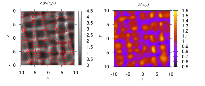
Snapshots of the pattern in Fig. 7 show the film thickness $h(x,y)$ and the average density $\langle\rho\rangle(x,y)$ at $t=100$. The latter varies between $\langle\rho\rangle_{\rm min}=0.1$ and $\langle\rho\rangle_{\rm max}=4.5$, in a much larger range than for the regular pattern in Fig. 5. One recognizes the underlying square pattern in the average density $\langle\rho\rangle(x,y)$ but the main lattice directions are tilted against each other. The height profile $h(x,y)$ looks even stronger perturbed. Still the elevated regions of the film surface (drops) are approximately arranged in a square lattice. Movie 2 shows how the tilted lattice planes in $\langle\rho\rangle(x,y)$ seem to split up and merge with their neighbors. The snapshot in Fig. 7 shows this scenario when going from left to right. This gives the whole pattern a highly dynamic appearance.

Figure 8: (Color online) Temporal evolution from the homogeneous state for parameters as in Fig. 7. (a) The mode type $M$, (b) the spectral density $S(\nu)$ of $M(t)$ on the interval $t\in[20,100]$, (c) the magnitude of the fluid flux, $\mid\bar{J}_{h}\mid=\sqrt{(\bar{J}_{h})_{x}^{2}+(\bar{J}_{h})_{y}^{2}}$, (d) the magnitude of the translational flux of the swimmers, $\mid\bar{J}_{t}\mid=\sqrt{(\bar{J}_{t})_{x}^{2}+(\bar{J}_{t})_{y}^{2}}$, and (e) the time-averaged power spectral density of the height profile obtained with Eq. (47) by averaging over the interval $t\in[50,100]$.

The temporal evolution of the pattern is visualized in Fig. 8(a)-(d). The mode type $M$ in plot (a) is positive and oscillates randomly about its average value of $M\approx 0.08$. In Fig. 8(b) we plot the spectral density $S(\nu)$ of $M(t)$ calculated on the interval $t\in[20,100]$. We find a clear maximum at the frequency $\nu_{\mathrm{max}}\approx 1.87$ with small width $\Delta\nu/\nu_{\mathrm{max}}\approx 0.1$, which corresponds to a period of $T=1/\nu_{\mathrm{max}}\approx 0.53$. The frequency $\nu_{\mathrm{max}}$ belongs to the pulsating pattern clearly recognizable in Movie 2. A second, broader peak is located at $\nu_{\mathrm{max}}\approx 2.3$ with width $\Delta\nu/\nu_{\mathrm{max}}\approx 0.2$. In addition, there exists a continuous background in $S(\nu)$, which gives the pattern its random dynamic appearance. Random oscillations of the magnitude of the fluid flux, $\mid\bar{J}_{h}\mid=\sqrt{(\bar{J}_{h})_{x}^{2}+(\bar{J}_{h})_{y}^{2}}$, [see Fig. 8(c)] and of the magnitude of the translational flux of the swimmers, $\mid\bar{J}_{t}\mid=\sqrt{(\bar{J}_{t})_{x}^{2}+(\bar{J}_{t})_{y}^{2}}$, [see Fig. 8(d)], indicate global propagation of the pattern at each instance of time. However, we find that the propagation direction randomly changes with time with no preferred direction as expected for square symmetry.

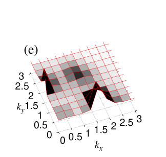
Finally, to reveal the periodic structure of the pattern, we determined the time-averaged power spectral density from Eq. (47) averaged over the time interval $t\in[50,100]$. As shown in Fig. 8(e), the spectral density has two major broad peaks: one is centered around $(k_{x}=2\pi m/L=1.57,\,k_{y}=2\pi k/L=0)$, i.e. $m=5$, $k=0$, and the other one is centered around $(k_{x}=2\pi m/L=0,\,k_{y}=2\pi k/L=1.57)$, i.e. $m=0$ and $k=5$. These peaks correspond to a square pattern with the main lattice directions aligned along the coordinate axes, i.e. $\Psi=0$ or $\Psi=\pi/2$. The dominating wave length or lattice constant $l_{w}$ of the pattern is $l_{w}=L/\sqrt{m^{2}+k^{2}}=20/5=4$. The third peak with much less intensity at $(k_{x}=2\pi m/L=1.25,k_{y}=2\pi k/L=1.88)$, i.e. $m=4$ and $k=6$, can roughly be interpreted as a contribution from the sum of the two major wave vectors spanning the reciprocal lattice.

IV.4 Multistability

In order to systematically study the occurence and stability of the two patterns studied in the previous sections, we follow these patterns in parameter space using a primitive “continuation method”. Namely, we take a snapshot of a converged (time-dependent) state at some parameter value and use it as initial condition for simulating the evolving pattern in a neighboring point in parameter space. The technique allows us to follow states, which are linearly stable, and thereby identify multistability in parameter space. Depending on the initial condition different stable spatio-temporal stable patterns are obtained. For an overview of proper continuation methods, which are also able to follow unstable steady states and therefore to determine the complete bifurcation diagram, see Refs. Kuznetsov (2010); Dijkstra et al. (2014). However, these methods are not readily available for time-periodic solutions of our PDE system.

Figure 9: (Color online) (a) The mode number $M$ during the continuation of the standing waves at fixed $V=3.5$ and $L=20$. Standing waves that emerged from the homogeneous steady state at $V=3.5$ and $D_{\rm eff}=6.175$ are numerically continued by increasing $D_{\rm eff}$. The vertical lines mark times when $D_{\rm eff}$ is changed. The respective values of $D_{\rm eff}$ for each interval are given by the numbers in each panel. The thick red solid line shows the mode type, averaged over one oscillation period. (b,c) Continuation of patterns with intermittent symmetry, emerged from the homogeneous steady state at $V=3.5$ and $D_{\rm eff}=600$ with $L=20$. Shown are (b) the mode number $M$ and (c) the modulus of the fluid flux $\sqrt{(\bar{J}_{h})_{x}^{2}+(\bar{J}_{h})_{y}^{2}}$ in dependence of time. The time axis is reversed.

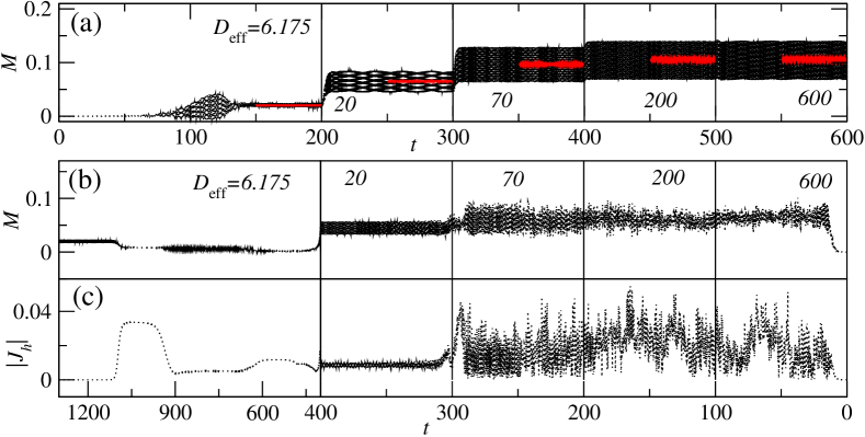
First, we start with the regular standing wave pattern, which we explored in Sec. IV.2 and in Fig. 5 at fixed $V=3.5$. We follow the standing wave solution along the line connecting points $2$ and $4$ in Fig. 2(a) by gradually decreasing $D$ (or increasing $D_{\rm eff}$) in steps using four distinct values, namely $D_{\rm eff}=6.175\rightarrow 20\rightarrow 70\rightarrow 200\rightarrow 600$. At each parameter point, we let the system settle into a stable state, which we identify by monotoring mode type $M(t)$ and fluid flux $\bar{J}_{h}$. The resulting time evolution of mode type $M$ during the continuation schedule is shown in Fig. 9(a). We find that the standing wave pattern keeps its main characteristics up to the largest value $D_{\rm eff}=600$ [point $4$ in Fig. 2(a)]. In particular, mode type $M$ shows regular oscillations. The mean value of $M$ [red solid line in Fig. 9(a)] and the oscillation amplitude of $M$ increase with $D_{\rm eff}$. They reach their respective maximal values of $0.1$ and $0.06$ at around $D_{\rm eff}=200$, where the density and height variations are more pronounced compared to Fig. 5. Furthermore, the oscillation period monotonically increases with $D_{\rm eff}$ (not shown). Interestingly, the spatial period of the pattern remains unchanged during the entire continuation schedule.

Next, we start with the strongly perturbed square pattern from Sec. IV.3 and Fig.7 and follow the same path in Fig. 2(a) but this time backward from point 4 to point 2. For consistency, we use the same values of $D_{\rm eff}$ as in Fig. 9(a). The time evolution of the mode type $M$ and the modulus of the fluid flux $\mid\bar{J}_{h}\mid$ are plotted in Figs. 9(b) and (c) with reversed time axis. Remarkably, the system reaches the regular standing wave pattern only for parameters close to the stability threshold, i.e., when $D_{\rm eff}$ is decreased to the value in point $2$ in Fig.2(a). After some transient dynamics, visible in the time intervall from $t=400$ to 1100 in Figs. 9(b) and (c), the system settles on the stable standing wave pattern.

For larger values of $D_{\rm eff}$, i.e., further away from the threshold, we found that the system is multistable. At $D_{\rm eff}>20$ stable regular standing waves still exist but also patterns similar to the strongly perturbed square pattern as shown in Fig.7 are stable. However, at $D_{\rm eff}=20$, the dynamics of the square pattern becomes more regular but still keeps the feature of lattice planes splitting and merging with their neighbors. This is demonstrated by Movie 3 and by the snapshots in Fig. 10(a) and (b), taken at $t=400$ during the numerical continuation in Fig. 9.

Figure 10: (Color online) (a,b) Persisting dynamic state at $V=3.5$ and $D_{\rm eff}=20$, during the numerical continuation of the patterns with intermittent symmetry in Fig.9. Snapshot taken at $t=400$. (c) The components of the translational surface flux $\bar{J}_{t}$. (d) the spectral density of $\mid\bar{J}_{h}\mid(t)$. (e) Time-averaged power spectral density of the pattern, obtained with Eq. (47) by averaging over the interval $t\in[350,400]$.

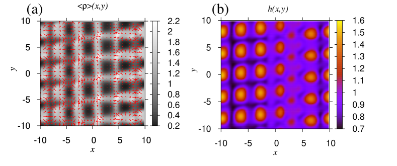
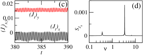
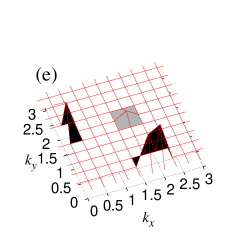
Figure 10(d) shows the $x$ and $y$ components of the translational flux of the swimmers. One clearly recognizes directed motion, on average, into the negative $x$ and positive $y$ direction, which is also visible in Movie 3. The components of the fluid flux $\bar{J}_{h}(t)$ behave similarly. Furthermore, both flux components show a fast oscillation with a weak slow modulation superimposed. By taking the Fourier transforms of $\mid\bar{J}_{h}(t)\mid$ [Fig. 10(d)], one identifies a dominant peak at $\nu=3.5$ corresponding to a period of $T=0.28$ of the fast oscillations. They result from the pulsation in the square pattern as Movie 3 demonstrates, in particular, for the height profile. The weak modulation generates a small peak in the power spectrum with frequency $\nu=0.36$ or period $T=2.8$. It is not really recognizable in the time evolution of Movie 3. Otherwise, the continuous part of the spectrum as observed in Fig. 8(b) for the strongly perturbed square pattern is missing here since the square pattern has a more regular dynamics.

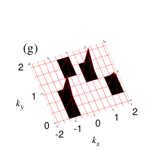
Finally, the time-averaged power spectral density $S_{h}$, averaged over the interval $t\in[350,400]$, is given in Fig. 10(e). The two major peaks correspond to the square pattern with spatial period of $L/6$ aligned along the coordinate axes. The third, much weaker peak at $k_{x}=k_{y}=2\pi m/L=1.57$ with $m=5$ again roughly corresponds to a contribution of the two major wave vectors spanning the reciprocal lattice.

Multistability of several persisting dynamic states under identical external conditions was also found in other systems. For example, in experiments on groups of schooling fish Tunstrøm et al. (2013) it was observed that depending on the starting conditions and/or the nature of perturbations, as well as the group size, the fish group may exhibit two different dynamic states: the so-called milling state, which is characterized by fish swimming in a large circle, and the polarised state, which corresponds to fish swimming predominantly in one direction.

IV.5 Persisting traveling patterns

Figure 11: (Color online) (a,b) Snapshots of the persisting traveling pattern, which emerges from the mixed instability type for $V=2$, $D=2.4$, ($D_{\rm eff}=0.88$), $L=20$ [see point $3$ in Fig. 2(a)]. The corresponding dispersion curve is shown in Fig. 2(d). (c) Mode type $M$, (d) $x$ and $y$ component of the space averaged fluid flux $\bar{\bm{J}}_{h}$, (e) the film height $h(t)$ at a randomly chosen point on the film surface, and (f) its power spectrum $S_{h}$. (g) Power spectrum for the spatial modulation of the height profile [see Eq. (47)] averaged over the interval $t\in[800,900]$.

In the triangular parameter region in Fig. 2, where the mixed instability occurs, one finds persisting patterns, i.e., long-time stable spatio-temporal patterns that are characterized by a time-independent mode type and a constant non-zero fluid flux, i.e., travelling waves. Figures 11(a) and (b) give example snapshots for such a pattern obtained at point $3$ in Fig. 2(a) at system size $L=20$ and at time $t=900$. Movie 4 reveals a pattern traveling approximately along the diagonal with a propagation speed estimated to be of the order of the self-propulsion velocity $V=2$. The maxima in the height profile form a rectangular lattice. Perturbations run along the lattice lines and shift the maxima by roughly half a lattice constant; presumably, to match the periodic boundary condition for the whole square domain. The time evolutions of mode type $M$ and of the components of the fluid flux, $(J_{h})_{x}$ and $(J_{h})_{y}$, are shown in Fig. 11(c) and (d), respectively. The height modulation at an arbitrary point plotted in Fig. 11(e) looks rather irregular. Its power spectrum in Fig. 11(f) reveals one peak at $\nu=0.32$, which corresponds to one shift motion of a bump in the height profile. Frequencies at $\nu=0.1$ and $0.17$ belong to longer cycles of two or three shifts. The power spectral density for the spatial modulations in the film height, averaged over the interval $t\in[800,900]$, is plotted in Fig. 11(g). In the upper and the lower halves of the snapshot in Fig. 11(b) one can clearly see a rectangular pattern with the aspect ratio of $\approx 1.3$. Remarkably, the aspect ratio of $\approx 1.3$ of the rectangular pattern is not compatible with the periodic boundary conditions of the square domain. Nontheless, the pattern is fitted into the square domain due to the presence of a defect-like modulation, seen at the center of the snapshot. The defect disturbes the rectangular lattice dynamically, as it continuously moves along the lattice lines and shifts the elevations in the height profile (see Movie 4). As a result, in the power spectrum in Fig. 11(g) we find two major peaks located at $\{k_{x}^{(1)}=0.62,k_{y}^{(1)}=1.25\}$ and $\{k_{x}^{(2)}=-0.94,k_{y}^{(2)}=0.62\}$ and one smaller peak located at $\{k_{x}^{(3)}=-0.94,k_{y}^{(3)}=0.31\}$. The remaining two weaker peaks are again higher contributions from wave vectors in the reciprocal lattice.

Persisting states characterized by propagating structures are well known for active matter systems. Thus, traveling density waves were found in experiments with an assay of actin filaments, driven by motor proteins Schaller et al. (2010). At the leading edge (lamellipodium) of a crawling cell, the alignment of actin filaments along the substrate leads to the forward translation of lamellipodium and thus, to cell motility Sma (2002). Moving density stripes and propagating isolated density clusters have been found in microscopic Vicsek-type models and in continuum models of self-propelled particles Chaté, H. et al. (2008); Gopinath et al. (2012); Mishra et al. (2010).

IV.6 Random patterns

Figure 12: (Color online) Random patterns emerge in the region of the zero wave number instability at $V=3.5$ and $D_{\mathrm{eff}}=0.66$ in a system of size $L=60$. Number of the Fourier modes for the discretisation in space is $N=128$.

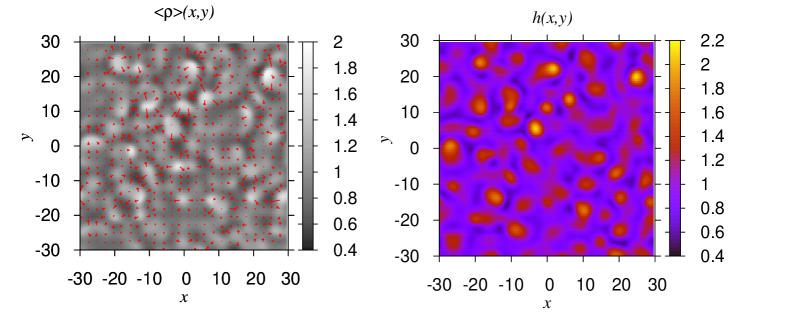
When studying the nonlinear behaviour for $V=3.5$ and $D_{\rm eff}=0.66$ [point $1$ in Fig. 2(a)], we find truly random patterns emerging from the zero wave-number instability. The corresponding dispersion curve is shown in Fig. 2(b) and gives the fastest growing wave length as $l_{\mathrm{max}}\approx 9$. We set $L=60$, $N=128$ and start the simulations at the trivial state. After a transient, the system settles to an irregular pattern in space and time that oscillates randomly and locally travels in random directions. Typical snapshots are shown in Fig. 12 and Movie 5 illustrates the irregular spatio-temporal pattern.

Figure 13: (Color online) (a) Time-averaged spectral density from Eq. (47) computed numerically by averaging the Fourier transformed film thickness patterns in Fig.12 over $t\in[150,350]$. (b,c) The mode type $M$ and the modulus of the fluid flux $\mid\bar{J}_{h}\mid$ over time. (d) Time evolution of $h(t)$ at a randomly chosen point on the film surface. (e) Spectral density $S_{h}$ of $h(t)$ from (d). (f) Normalised radial autocorrelation function $C(r)$. Inset shows zoomed graph of $C(r)$ around zero.

The randomness of the pattern is clearly visible in the time evolution of mode type $M$ and of the modulus of the fluid flux $\mid\bar{J}_{h}\mid$, which we plot in Figs. 13(a) and (b), respectively. In Fig. 13(a) the power spectral density of the height profile averaged over the interval $t\in[150,350]$ reveals a clear maximum at $\mid{\bm{k}}\mid=0.7$. The spectral density is radially symmetric, which implies that spatial correlations in the pattern only depend on the distance $r$ between any two points on the film surface. Otherwise, it is continuous as expected for a random pattern. Via the convolution theorem, the time-averaged power spectral density from Eq. (47) is directly related to the spatial height correlation function

$$C({\bm{r}})=\frac{C_{0}}{t_{2}-t_{1}}\int_{t_{1}}^{t_{2}}dt\,\int[h({\bm{r}}+{\bm{w}})-1][h({\bm{w}})-1]\,d{\bm{w}},$$ (48)

where $t_{1}=150$ and $t_{2}=350$ and the constant $C_{0}$ is chosen such that $C(0)=1$. We plot the normalised radially-symmetric correlation function $C(r)$ in Fig. 13(f) over the length of half the system size, i.e., $L/2=30$. $C(r)$ rapidly decreases with $r$ and drops by two orders of magnitude over the distance of $r=10$, as shown in the inset of Fig. 13(f). Correlations become negligibly small at distances larger than 10 and the pattern looks random. The oscillation at small distances corresponds to the maximum in the power spectral density. They are caused by wave fronts traveling in random directions, which one recognizes in the orientation-averaged swimmer density in Movie 5.

Finally, the film height at an arbitrary position changes randomly in time, as shown in Fig. 13(d). However, the spectral density $S_{h}$ plotted in Fig. 13(e) has a clear peak at $\nu=0.055$. This implies that the temporal dynamics of the patterns cannot be regarded as purely random.

Highly dynamic random spatio-temporal patterns of active matter are known as quasi or mesoscale turbulence. Irregular turbulent states have been found in experiments with dense bacterial suspensions Dunkel et al. (2013a); Lushia et al. (2005); Sokolov et al. (2007); Sokolov and Aranson (2012); Liu and I (2012); Sokolov et al. (2009); Wensink et al. (2012); Ishikawa et al. (2011) and in active microtubuli networksSanchez et al. (2012).

V Discussion and Conclusion

We have investigated the collective behaviour of a colony of point-like non-interacting self-propelled particles (microswimmers) that swim at the free surface of a thin liquid layer on a solid support. In contrast to former work Alonso and Mikhailov (2009), where the motion of the particles was considered to be purely orthogonal to the free surface, here we have also allowed for active motion parallel to the film surface. The resulting coupled dynamics of the swimmer density $\rho(x,y,\phi,t)$ and the film thickness profile $h(x,y,t)$ is captured in a long-wave model in the form of a Smoluchowski equation for the one-particle density $\rho(x,y,\phi,t)$ and a thin film equation for $h(x,y,t)$ that allows for (i) diffusive and convective transport of the swimmers (including rotational diffusion), (ii) capillarity effects (Laplace pressure) including a Marangoni force caused by gradients in the swimmer density, (iii) and a vertical pushing force of the swimmers that acts onto the liquid-gas interface.

First, we have extended the linear stability analysis of the homogeneous and isotropic state that was presented before in Ref. Pototsky et al. (2014) focusing, in particular, on the characteristics of the two instability modes (one at zero wave number and one at finite wave number) and their mixed appearance close to the border of the stable region in the stability diagram spanned by the swimmer speed $V$ and the effective diffusion constant $D_{\mathrm{eff}}$.

Our linear stability analysis indicates that the onset and dispersion relation of the zero-wave number instability mode do not fit well into the classification scheme of Cross and Hohenberg Cross and Hohenberg (1993). The long-wave instability of the free film surface occurs at $k=0$, where the zero-wave number mode has zero imaginary part. However, arbitrarily close to onset in the unstable region, the fastest growing wave number $k_{\rm max}$ corresponds to a pair of complex conjugate eigenvalues. Moreover, the entire unstable band of wave numbers, $0<k<k_{c}$, does always contain a range of small $k<k_{\mathrm{rc}}\sim|\eta|$ (with $\eta$ measuring the distance from the stability threshold), where the first two leading eigenvalues are real (one $\sim k^{2}$ and one $\sim k^{4}$), and a range $k_{\rm rc}<k<k_{c}$, where the two leading eigenvalues form a complex conjugate pair. The latter range always contains the fastest growing wave number $k_{\mathrm{max}}$. This indicates that this zero-wave number instability is similar to a zero-frequency Hopf bifurcation in dynamical systems Kuznetsov (2010) and in the context of the instabilities of spatially extended systems, it might be called a zero-frequency type $II_{o}$ instability.

The behaviour at about $k=0$ has also important implications for a weakly nonlinear theory for the short-wave instability at $k=k_{c}$. Such a theory would need to take into account that the slow complex modes around $k=k_{c}$ couple to the two unstable long-wave modes at $k\approx 0$ with real eigenvalues. We believe that such a coupling is responsible for the observed wave behaviour, where a travelling wave is perturbed by a long-wave modulation, as in Fig.10. The two long-wave modes are a direct consequence of the existing two conserved quantities in the system: the mean film height and the orientation-averaged mean swimmer concentration. Simpler cases with one long-wave mode (resulting from a single conserved quantity) that couples to a short-wave mode have been considered in Refs. Matthews and Cox (2000); Cox and Matthews (2003); Winterbottom et al. (2005). Such an analysis is not feasible in our case, where the evolution equations capture the dynamics in two spatial dimensions and account for a fully $\phi$-dependent density $\rho(x,y,\phi,t)$. However, a one-dimensional model system, where instead of rotational diffusion the swimmers can only flip between swimming to the left or right shows similar transitions and lends itself to a weakly nonlinear analysis. Such a simplified system is under investigation and will be presented elsewhere.

Numerical simulations of the time evolution equations (8) and (12) reveal a rich variety of persisting dynamic states. We have abstained from a comprehensive parameter study of the different persisting states. Instead, we have given an overview of the zoo of dynamic states that can be found, when solving the system of equations (8) and (12).

In particular, for parameters chosen in the vicinity of the stability threshold of the finite wave number instability, we have found a highly regular dynamic standing wave pattern by starting the simulations with small random perturbations of the trivial state. The standing wave pattern is characterised by a regular array of elevations of the free film surface that periodically transform and rearrange following a rather complex pathway. Thus, over one quarter of the oscillation cycle, the elevations transform from a perfect square lattice into an array of stripes followed by a new square lattice of elevations that is shifted w.r.t. the initial square lattice by exactly one half of the spatial wave period. The transformation of the average density of swimmers follows the pattern of the film thickness profile. The swimmers are arranged in a regular lattice with high and low density spots. Spatial variations of the film thickness profile and the orientation-averaged density profile are in-phase implying that high density spots sit approximately on top of the droplets. The orientation of swimmers in each high density spot shows strong polar order with a hedgehog defect right at the maximum. The space-averaged fluid flux of the square wave is zero at all times.

Next, we have employed a ’primitive’ continuation method and followed the standing wave patterns through parameter space moving further away from the stability threshold. Our numerical results suggest that standing wave patterns exist and are stable possibly in the entire region, where the homogeneous state is linearly unstable w.r.t. the finite wave number instability (i.e. for $D_{\rm eff}>1$). On the reverse path, initial random perturbations of the homogeneous and isotropic state develop into a strongly perturbed square pattern, where lattice lines continuously split and merge with their neighbors. Unlike for the regular standing wave pattern, the average fluid flux oscillates randomly about zero. However, the time-averaged power spectral density of the height profile reveals a clear square pattern. Further decreasing $D_{\rm eff}$ towards the stability threshold, the dynamics of the perturbed square lattice becomes regular. The fluid flux in this state is periodic in time with a weak modulation superimposed. The major frequency corresponds to a pulsation of the square pattern.

By choosing the parameters in the mixed-instability region, we find a persisting traveling pattern characterised by constant space-averaged fluid flux. Elevations in the film surface are arranged in a rectangular lattice that travels in one direction with the speed of the order of the self-propulsion velocity, while perturbations continuously shift the hight elevations. At their positions the swimmers form high-density spots with strong polar order around a hedgehog defect similar to the regular standing wave. Finally, choosing parameters from the region with the zero wave number instability, one finds a random spatio-temporal pattern with a correlation length much smaller than the system size.

Our findings clearly show that a rich variety of persisting regular and irregular dynamic states can be found in an active matter system of self-propelled particles without direct interactions. In our model, the interaction between the swimmers occurs on a coarse-grained level and is mediated by large-scale deformations of the liquid film. Similar types of dynamic states found here were previously observed in other active matter systems of interacting particles as indicated at the respective ends of sections IV.2 to IV.6. For instance, stable square patterns were found in Vicsek-type models with memory Nagai et al. (2015). Multistability of the system under identical external conditions was reported earlier in experiments with groups of schooling fish Tunstrøm et al. (2013). Various traveling states occurred in experiments with motility assays of actin filaments driven by motor proteins Schaller et al. (2010), in microscopic Vicsek-type models, and in continuum models of self-propelled particles Chaté, H. et al. (2008); Gopinath et al. (2012); Mishra et al. (2010). Finally, random or turbulent states were observed in experiments with dense bacterial suspensions Dunkel et al. (2013a); Lushia et al. (2005); Sokolov et al. (2007); Sokolov and Aranson (2012); Liu and I (2012); Sokolov et al. (2009); Wensink et al. (2012); Ishikawa et al. (2011) and in active microtubule networks Sanchez et al. (2012). It is fascinating that active particles acting as surfactants at the surface of a thin liquid film provide a model system, where all these different dynamic patterns can be realized by tuning appropriate parameters.

Possible extensions of the model include the incorporation of wettability effects by adding the Derjaguin (disjoining) pressure to study swimmer carpets not only on films but also on shallow droplets and, in particular, interactions with (moving) contact lines. One may also go beyond the approximation of point-like non-interacting particles by introducing finite size effects (short-range interactions between particles) as well as long-range (hydrodynamic) interactions. The resulting Smoluchowski equation would then contain non-local terms as in dynamical density functional theories for the diffusive dynamics of interacting colloids, polymers, and macromolecules Marconi and Tarazona (1999); Archer and Evans (2004). For a consistent model also the film height equation would require additional terms that may be determined via the gradient dynamics formulation Thiele et al. (2012) that has to be recovered in the limit of passive surfactant particles/molecules.

VI Appendix: Semi-implicit numerical scheme for Eqs. (12,8)

In the employed dimensionless quantities, the resulting coupled system consists of the reduced Smoluchowski equation and the thin film equation. It reads

$$\partial_{t}h + {\bm{\nabla}}\cdot{\bm{J}}_{h}=0,$$

$$\partial_{t}\rho + {\bm{\nabla}}\cdot{\bm{J}}_{\rm t}+\partial_{\phi}J_{\phi}=0,$$ (49)

with the dimensionless fluid flux ${\bm{J}}_{h}$, the translational and rotational probability currents ${\bm{J}}_{t}$ and $J_{\phi}$, the surface fluid velocity ${\bm{U}}_{\parallel}$ and the vorticity of the fluid flow $\Omega_{z}$

$${\bm{J}}_{h} = \frac{h^{3}}{3}{\bm{\nabla}}\left[\Delta h+\beta\langle\rho\rangle\right]-\frac{1}{2}\left(h^{2}{\bm{\nabla}\langle\rho\rangle}\right),$$

$${\bm{J}}_{\rm t} = \left(V{\bm{q}}+{\bm{U}}_{\parallel}-d{\bm{\nabla}}\right)\rho,$$

$$J_{\phi} = \frac{1}{2}\Omega_{z}\rho-D\partial_{\phi}\rho,$$

$${\bm{U}}_{\parallel} = -h{\bm{\nabla}}\langle\rho\rangle+\frac{h^{2}}{2}{\bm{\nabla}}\left(\Delta h+\beta\langle\rho\rangle\right),$$

$$\Omega_{z} = \partial_{x}U_{y}-\partial_{y}U_{x}.$$ (50)

The coupled Eqs. (VI) are solved numerically using the following version of the semi-implicit spectral method. First, we average the density equation over the orientation angle $\phi$. This yields

$$\partial_{t}\langle\rho\rangle + {\bm{\nabla}}\cdot\langle{\bm{J}}_{\rm trans}\rangle=0,$$ (51)

with the average translational current $\langle{\bm{J}}_{\rm trans}\rangle=V\langle{\bm{q}}\rho\rangle+({\bm{U}}-d{\bm{\nabla}})\langle\rho\rangle$ and ${\bm{q}}=(\cos{\phi},\sin{\phi})$. It is worthwhile noticing that the only term in Eq. (51) that depends on the three-dimensional density $\rho(x,y,\phi,t)$ is the average orientation vector $\langle{\bm{q}}\rho\rangle$. All other terms in Eq. (51), including the surface fluid velocity ${\bm{U}}$ explicitly depend on the average density $\langle\rho\rangle$.

Next, we group the thin film equation together with Eq. (51)

$$\partial_{t}h + {\bm{\nabla}}\cdot{\bm{J}}_{h}=0,$$

$$\partial_{t}\langle\rho\rangle + {\bm{\nabla}}\cdot\langle{\bm{J}}_{\rm trans}\rangle=0,$$ (52)

with the fluid flux ${\bm{J}}_{h}=\frac{h^{3}}{3}{\bm{\nabla}}\left[\Delta h+\beta\langle\rho\rangle\right]-\frac{1}{2}{\bm{\nabla}}\left(h^{2}{\bm{\nabla}\langle\rho\rangle}\right)$.

At the next step, we single out the linear parts in all the terms in Eqs. (VI) that explicitly depend on the average density $\langle\rho\rangle$. This is done by linearising the current ${\bm{J}}_{t}$ and the fluid flux ${\bm{J}}_{h}$ about the trivial steady state given by $h=1$ and $\langle\rho\rangle=1$.

Finally, following the standard implicit time-integration scheme, we replace $\partial_{t}h$ and $\partial_{t}\langle\rho\rangle$ by $(h^{t+dt}-h^{t})/dt$ and by $(\langle\rho\rangle^{t+dt}-\langle\rho\rangle^{t})/dt$, respectively and take all linear terms at time $t+dt$ and all nonlinear terms, including the term $V\langle{\bm{q}}\rho\rangle$, at time $t$. Upon these transformations Eqs. (VI) become

$$\frac{h^{t+dt}-h^{t}}{dt} + \frac{1}{3}\Delta^{2}h^{t+dt}+\left(\frac{\beta}{3}-\frac{1}{2}\right)\Delta\langle\rho\rangle^{t+dt}+{\bm{\nabla}}\cdot({\bm{N}L}_{h})^{t}=0,$$

$$\frac{\langle\rho\rangle^{t+dt}-\langle\rho\rangle^{t}}{dt} + \frac{1}{2}\Delta^{2}h^{t+dt}+\left(\frac{\beta}{2}-1-d\right)\Delta\langle\rho\rangle^{t+dt}+{\bm{\nabla}}\cdot(\langle{\bm{N}L}_{\rm trans}\rangle)^{t}=0,$$ (53)

with the nonlinear parts given by

$$({\bm{N}L}_{h})^{t} = \left[\frac{h^{3}-1}{3}{\bm{\nabla}}\left[\Delta h+\beta\langle\rho\rangle\right]-\frac{1}{2}{\bm{\nabla}}\left([h^{2}-1]{\bm{\nabla}\langle\rho\rangle}\right)\right]^{t},$$

$$(\langle{\bm{N}L}_{\rm trans}\rangle)^{t} = \left[V\langle{\bm{q}}\rho\rangle+({\bm{U}})\langle\rho\rangle-\frac{1}{2}{\bm{\nabla}}(\Delta h)-\left(\frac{\beta}{2}-1\right){\bm{\nabla}}\langle\rho\rangle\right]^{t}.$$ (54)

After taking the discrete Fourier transforms of Eqs. (VI), we find the updated fields $h^{t+dt}$ and $\langle\rho\rangle^{t+dt}$ at the time step $t+dt$.

With the update average density $\langle\rho\rangle^{t+dt}$ and the film thickness $h^{t+dt}$ at hand, we find the updated surface fluid velocity ${\bm{U}}^{t+dt}$ and the updated vorticity $\Omega^{t+dt}$. These functions are then substituted into the three-dimensional density equation

$$\frac{\rho^{t+dt}-\rho^{t}}{dt} + {\bm{\nabla}}\cdot{\bm{J}}_{\rm trans}+\partial_{\phi}J_{\rm rot}=0,$$ (55)

with the translational current ${\bm{J}}_{\rm trans}=V({\bm{q}}\rho)^{t}+({\bm{U}}^{t+dt})\rho^{t}-d{\bm{\nabla}}\rho^{t+dt}$ and the rotational current $J_{\phi}=(1/2)\Omega^{t+dt}\rho^{t}-D(\partial_{\phi}\rho^{t+dt})$.

After taking the Fourier transform of Eq. (55) both, in space as well as in the angle $\phi$, we find the updated three-dimensional density $\rho^{t+dt}$.

References

- Ramaswamy (2010) S. Ramaswamy, Annu. Rev. Condens. Matter Phys. 1, 323 (2010).
- Marchetti et al. (2013) M. Marchetti, J. Joanny, S. Ramaswamy, T. Liverpool, J. Prost, M. Rao, and R. Simha, Rev. Mod. Phys. 85 (2013).
- Buttinoni et al. (2013) I. Buttinoni, J. Bialké, F. Kümmel, H. Löwen, C. Bechinger, and T. Speck, Phys. Rev. Lett. 110, 238301 (2013).
- Theurkauff et al. (2012) I. Theurkauff, C. Cottin-Bizonne, J. Palacci, C. Ybert, and L. Bocquet, Phys. Rev. Lett. 108, 268303 (2012).
- Palacci et al. (2010a) J. Palacci, C. Cottin-Bizonne, C. Ybert, and L. Bocquet, Phys. Rev. Lett. 105, 088304 (2010a).
- Palacci et al. (2013) J. Palacci, S. Sacanna, A. P. Steinberg, D. J. Pine, and P. M. Chaikin, Science 339, 936 (2013).
- Thutupalli et al. (2011) S. Thutupalli, R. Seemann, and S. Herminghaus, New Journal of Physics 13, 073021 (2011).
- Riedel et al. (2005) I. H. Riedel, K. Kruse, and J. Howard, Science 309, 300 (2005).
- Dombrowski et al. (2004a) C. Dombrowski, L. Cisneros, S. Chatkaew, R. E. Goldstein, and J. Kessler, Phys. Rev. Lett. 93, 098103 (2004a).
- Lushia et al. (2005) E. Lushia, H. Wioland, and R. E. Goldstein, PNAS 111, 9733 (2005).
- Sokolov et al. (2007) A. Sokolov, I. S. Aranson, J. O. Kessler, and R. E. Goldstein, Phys. Rev. Lett. 98, 158102 (2007).
- Sokolov and Aranson (2012) A. Sokolov and I. S. Aranson, Phys. Rev. Lett. 109, 248109 (2012).
- Liu and I (2012) K.-A. Liu and L. I, Phys. Rev. E 86, 011924 (2012).
- Sokolov et al. (2009) A. Sokolov, R. E. Goldstein, F. I. Feldchtein, and I. S. Aranson, Phys. Rev. E 80, 031903 (2009).
- Wensink et al. (2012) H. H. Wensink, J. Dunkel, S. Heidenreich, K. Drescher, R. E. Goldstein, H. Löwen, and J. M. Yeomans, PNAS 109, 14308 (2012).
- Ishikawa et al. (2011) T. Ishikawa, N. Yoshida, H. Ueno, M. Wiedeman, Y. Imai, and T. Yamaguchi, Phys. Rev. Lett. 107, 028102 (2011).
- Dombrowski et al. (2004b) C. Dombrowski, L. Cisneros, S. Chatkaew, R. E. Goldstein, and J. O. Kessler, Phys. Rev. Lett. 93, 098103 (2004b).
- Schwarz-Linek et al. (2012) J. Schwarz-Linek, C. Valeriani, A. Cacciuto, M. E. Cates, D. Marenduzzo, A. N. Morozov, and W. C. K. Poon, PNAS 109, 4052 (2012).
- Dunkel et al. (2013a) J. Dunkel, S. Heidenreich, K. Drescher, H. H. Wensink, M. Bär, and R. E. Goldstein, Phys. Rev. Lett. 110, 228102 (2013a).
- Schaller et al. (2010) V. Schaller, C. Weber, C. Semmrich, E. Frey, and A. R. Bausch, Nature 467, 73 (2010).
- Surrey et al. (2001) T. Surrey, F. Nédélec, S. Leibler, and E. Karsenti, Science 292, 1167 (2001).
- Sumino et al. (2012) Y. Sumino, K. H. Nagai, Y. Shitaka, D. Tanaka, K. Yoshikawa, H. Chate, and K. Oiwa, Nature 483, 448 (2012).
- Derenyi and Vicsek (1995) I. Derenyi and T. Vicsek, Phys. Rev. Lett. 75, 374 (1995).
- Bricard et al. (2013) A. Bricard, J.-B. Caussin, N. Desreumaux, O. Dauchot, and D. Bartolo, Nature 503, 95 (2013).
- Nagai et al. (2015) K. H. Nagai, Y. Sumino, R. Montagne, I. S. Aranson, and H. Chaté, Phys. Rev. Lett. 114, 168001 (2015).
- Großmann et al. (2014) R. Großmann, P. Romanczuk, M. Bär, and L. Schimansky-Geier, Phys. Rev. Lett. 113, 258104 (2014).
- Lauga and Powers (2009) E. Lauga and T. R. Powers, Rep. Prog. Phys. 72, 096601 (2009).
- Bialke et al. (2013) J. Bialke, H. Löwen, and T. Speck, EPL (Europhysics Letters) 103, 30008 (2013).
- Peruani et al. (2006) F. Peruani, A. Deutsch, and M. Bär, Phys. Rev. E 74, 030904 (2006).
- Baskaran and Marchetti (2008) A. Baskaran and M. C. Marchetti, Phys. Rev. E 77, 011920 (2008).
- van Teeffelen and Löwen (2008) S. van Teeffelen and H. Löwen, Phys. Rev. E 78, 020101(R) (2008).
- (32) A. Zöttl and H. Stark, Phys. Rev. Lett. 112, 118101 (2014).
- (33) M. Hennes, K. Wolff, and H. Stark, Phys. Rev. Lett. 112, 238104 (2014).
- (34) O. Pohl and H. Stark, Phys. Rev. Lett. 112, 238303 (2014).
- (35) O. Pohl and H. Stark, Eur. Phys. J. E 38, 93 (2015),
- Aranson et al. (2007) I. S. Aranson, A. Sokolov, J. O. Kessler, and R. E. Goldstein, Phys. Rev. E 75, 040901 (2007).
- Subramanian and Koch (2009) G. Subramanian and D. L. Koch, J. Fluid Mech. 632, 359 (2009).
- Thiele et al. (2012) U. Thiele, A. J. Archer, and M. Plapp, Phys. Fluids 24, 102107 (2012).
- Alonso and Mikhailov (2009) S. Alonso and A. Mikhailov, Phys. Rev. E 79, 061906 (2009).
- Pototsky et al. (2014) A. Pototsky, U. Thiele, and H. Stark, Phys. Rev. E 90, 030401(R) (2014).
- Oron et al. (1997) A. Oron, S. Davis, and S. Bankoff, Rev. Mod. Phys. 69, 931 (1997).
- Schwartz et al. (1995) L. W. Schwartz, D. E. Weidner, and R. R. Eley, Langmuir 11, 3690 (1995).
- Garbin et al. (2012) V. Garbin, J. C. Crocker, and K. J. Stebe, Langmuir 28, 1663 (2012).
- Alizadehrad et al. (2015) D. Alizadehrad, T. Krüger, M. Engstler, and H. Stark, PLoS Comput Biol 11, e1003967 (2015).
- Howse et al. (2007) J. R. Howse, R. A. L. Jones, A. J. Ryan, T. Gough, R. Vafabakhsh, and R. Golestanian, Phys. Rev. Lett. 99, 048102 (2007).
- Helden et al. (2015) L. Helden, R. Eichhorn, and C. Bechinger, Soft Matter 11, 2379 (2015).
- Lee et al. (2014) T. Lee, M. Alarcon-Correa, C. Miksch, K. Hahn, J. Gibbs, and P. Fischer, Nano Lett. 14, 2407 (2014).
- Enculescu and Stark (2011) M. Enculescu and H. Stark, Phys. Rev. Lett. 107, 058301 (2011).
- Wolff et al. (2013) K. Wolff, A. Hahn, and H. Stark, Eur. Phys. J. E 36, 43 (2013), ISSN 1292-8941.
- Gardiner (2004) C. W. Gardiner, Handbook of Stochastic Methods (Springer-Verlag, Berlin Heidelberg, 2004).
- Pototsky and Stark (2012) A. Pototsky and H. Stark, EPL (Europhysics Letters) 98, 50004 (2012).
- (52) Note that can also be introduced as , where denotes the vertical component of the fluid vorticity in the bulk of the film. The difference between and with from Eq.(13) is of the second order in parameter of the long-wave approximation, and thus, does not effect the results of the linear stability of the homogeneous steady state. However, certain aspects of the nonlinear evolution may vary depending on the definition of .
- Stellamanns et al. (2014) E. Stellamanns, S. Uppaluri, A. Hochstetter, N. Heddergott, M. Engstler, and T. Pfohl, Sci. Rep. 4 (2014).
- Palacci et al. (2010b) J. Palacci, C. Cottin-Bizonne, C. Ybert, and L. Bocquet, Phys. Rev. Lett. 105, 088304 (2010b).
- ten Hagen et al. (2011) B. ten Hagen, S. van Teeffelen, and H. Löwen, J. Phys.: Condes Matter 23, 194119 (2011).
- Golestanian (2012) R. Golestanian, Phys. Rev. Lett. 108, 038303 (2012).
- Beltrame and Thiele (2010) P. Beltrame and U. Thiele, SIAM J. Appl. Dyn. Syst. 9, 484 (2010).
- Grossmann et al. (2015) R. Grossmann, P. Romanczuk, M. Bar, and L. Schimansky-Geier, Eur. Phys. J.-Spec. Top. 224, 1325 (2015).
- Ziebert (2006) F. Ziebert, Ph.D. thesis, Universität Bayreuth (2006).
- Ziebert and Zimmermann (2005) F. Ziebert and W. Zimmermann, Eur. Phys. J. E 18, 41 (2005).
- Cross and Hohenberg (1993) M. C. Cross and P. C. Hohenberg, Rev. Mod. Phys. 65, 851 (1993).
- Dunkel et al. (2013b) J. Dunkel, S. Heidenreich, M. Bär, and R. E. Goldstein, New Journal of Physics 15, 045016 (2013b).
- Bestehorn (2006) M. Bestehorn, Hydrodynamik und Strukturbildung: Mit einer kurzen Einfuhrung in die Kontinuumsmechanik (Springer-Lehrbuch) (German Edition) (Springer, 2006), ISBN 3540337962.
- Kuznetsov (2010) Y. A. Kuznetsov, Elements of Applied Bifurcation Theory (Springer, New York, 2010), 3rd ed.
- Dijkstra et al. (2014) H. A. Dijkstra, F. W. Wubs, A. K. Cliffe, E. Doedel, I. F. Dragomirescu, B. Eckhardt, A. Y. Gelfgat, A. Hazel, V. Lucarini, A. G. Salinger, et al., Commun. Comput. Phys. 15, 1 (2014).
- Tunstrøm et al. (2013) K. Tunstrøm, Y. Katz, C. C. Ioannou, C. Huepe, M. J. Lutz, and I. D. Couzin, PLoS Comput Biol 9 (2013).
- Sma (2002) Trends in Cell Biology 12, 112 (2002), ISSN 0962-8924.
- Chaté, H. et al. (2008) Chaté, H., Ginelli, F., Grégoire, G., Peruani, F., and Raynaud, F., Eur. Phys. J. B 64 (2008).
- Gopinath et al. (2012) A. Gopinath, M. F. Hagan, M. C. Marchetti, and A. Baskaran, Phys. Rev. E 85, 061903 (2012).
- Mishra et al. (2010) S. Mishra, A. Baskaran, and M. C. Marchetti, Phys. Rev. E 81, 061916 (2010).
- Sanchez et al. (2012) T. Sanchez, D. T. N. Chen, S. J. DeCamp, M. Heymann, and Z. Dogic, Nature 491, 431 (2012).
- Kuznetsov (2004) Y. Kuznetsov, Elements of Applied Bifurcation Theory (Springer-Verlag, New York, 2004).
- Matthews and Cox (2000) P. C. Matthews and S. M. Cox, Nonlinearity 13, 1293 (2000).
- Cox and Matthews (2003) S. M. Cox and P. C. Matthews, Physica D 175, 196 (2003).
- Winterbottom et al. (2005) D. Winterbottom, P. Matthews, and S. Cox, Nonlinearity 18, 1031 (2005).
- Marconi and Tarazona (1999) U. M. B. Marconi and P. Tarazona, J. Chem. Phys. 110, 8032 (1999).
- Archer and Evans (2004) A. J. Archer and R. Evans, J. Chem. Phys. 121, 4246 (2004).