1 Introduction

A problem that tends to be ignored in the statistical analysis of experimental data in the language sciences is that responses often constitute time series, which raises the problem of autocorrelated errors. If the errors indeed show autocorrelational structure, evaluation of the significance of predictors in the model becomes problematic due to potential anti-conservatism of p-values.

This paper illustrates two tools offered by Generalized Additive Mixed Models (gamms) (Lin and Zhang,, 1999; Wood,, 2006, 2011, 2013) for dealing with autocorrelated errors, as implemented in the current version of the fourth author's mgcv package (1.8.9): the possibility to specify an ar(1) error model for Gaussian models, and the possibility of using factor smooths for random-effect factors such as subject and item. These factor smooths are set up to have the same smoothing parameters, and are penalized to yield the non-linear equivalent of random intercepts and random slopes in the classical linear framework.

Three examples illustrate the possibilities offered by gamms. First, a standard chronometric task, word naming, is examined, using data originally reported in Tabak, (2010). In this task, and similar tasks such as lexical decision, a participant is asked to respond to stimuli presented sequentially. The resulting sequence of responses constitute a time series in which the response at time $t$ may not be independent from the response at time $t-1$. For some participants, this non-independence may stretch across 20 or more lags in time. Second, a study investigating the pitch contour realized on English three-constituent compounds (Koesling et al.,, 2012) is re-examined. As pitch changes relatively slowly and relatively continuously, autocorrelation structure is strongly present. A reanalysis that brings the autocorrelation under statistical control leads to conclusions that differ substantially from those of the original analysis. The third case study follows up on a model reported by DeCat et al., (2014, 2015) fitted to the amplitude over time of the brain's electrophysiological response to visually presented compound words. We begin with a short general introduction to gamms.

2 Generalized additive mixed models

Generalized additive mixed models extend the generalized linear mixed model with a large array of tools for modeling nonlinear dependencies between a response variable and one or more numeric predictors. For nonlinear dependencies involving a single predictor, thin plate regression splines are available. Thin plate regression splines (tprs) model the response by means of a weighted sum of smooth regular basis functions that are chosen such that they optimally approximate the response, if that response is indeed a smooth function. The basis functions of tprs have much better mathematical properties compared to basis functions that are simple powers of the predictor (quadratic or higher-order polynomials). Importantly, the smoother is penalized for wiggliness, such that when fitting a gamm, an optimal balance is found between undersmoothing and oversmoothing.

When a response depends in a nonlinear way on two or more numeric predictors that are on the same scale, tprs can also be used to fit wiggly regression surfaces or hypersurfaces, approximated by means of weighted sums of regular surfaces which are again penalized for wiggliness. When predictors are not isometric, tensor product smooths should be used. Tensor product smooths (tps) approximate a wiggly surface or hypersurface using as basis functions restricted cubic splines, again with penalization for wiggliness.

Interactions of numerical predictors with a factorial predictor can be accomodated in two ways. One option is to fit a different wiggly line or surface for each level of such a factor. Alternatively, one may want to take one of the factor levels as reference level, fit a smooth for the reference level, and then fit difference curves or difference surfaces for the remaining factor levels. These difference curves have an interpretation similar to treatment contrasts for dummy coding of factors: The difference curve for level $k$, when added to the curve for the reference level, results in the actual predicted curve for factor level $k$.

When a factor has many different levels, as is typically the case for random-effect factors, it may be desirable to require the individual smooths for the different factor levels to have the same smoothing parameter. Together with a heavier penalty for moving away from zero, the resulting `factor smooths' are the nonlinear equivalent of the combination of random intercepts and random slopes in the linear mixed model.

In what follows, examples are discussed using R, which follows Wilkinson and Rogers, (1973) for the specification of statistical models. Extensions to the notation for model formulae made within the context of the package for linear mixed models (lme4, Bates et al.,, 2015) and the mgcv package for generalized additive mixed models (Wood,, 2006, 2011) are explained where used first.

3 Time series in a word naming task

Although there is awareness in the field of inter-trial dependencies in chronometric behavioral experiments (Broadbent,, 1971; Welford,, 1980; Sanders,, 1998; Taylor and Lupker,, 2001), efforts to take such dependencies into account are scarce. De Vaan et al., (2007) and Baayen and Milin, (2010) attempted to take the autocorrelation out of the residual error by including as a covariate the response latency elicited at the preceding trial. This solution, however, although effective, is not optimal from a model-building perspective, as the source of the autocorrelation is not properly separated out from the other factors that co-determine the response latency at the preceding timestep.

To illustrate the phenomenon, consider data from a word naming study on Dutch (Tabak,, 2010), in which subjects were shown a verb on a computer screen, and were requested to read out loud the corresponding past (or present) tense form. The upper row of panels of Figure 1 presents the autocorrelation function for selected, exemplary, subjects. The autocorrelation function presents, for lags 0, 1, 2, 3, …the correlation coefficient obtained when the vector of responses $\boldmath{v}_{1}$ at trials 1, 2, 3, …is correlated with the vector of responses $\boldmath{v}_{l}$ at trials 1+l, 2+l, 3+l, …($l>=0$). At lag $l=0$, the correlation is necessarily 1. As the lag increases, the correlation tends to decrease. For some subjects, there is significant autocorrelation at short lags, as illustrated in the first two panels. The subject in the third panel shows a ``seasonal'' effect, with an initial positive correlation morphing into a negative correlation around lag 10. The subjects in the next two panels show a very different pattern, with autocorrelations persisting across more than 20 lags.

Figure 1: Autocorrelation functions for the residuals of selected participants in the word naming task: top: observed response latencies; second row: residuals of a linear mixed-effects model with random by-participant intercepts and slopes for Trial; third row: residuals of a gamm with by-participant wiggly curves; fourth row: residuals of a gamm with by-participant wiggly curves and correction for ar(1) with $\rho=0.3$. Significant autocorrelations are shown in red, non-significant autocorrelations are presented in blue.

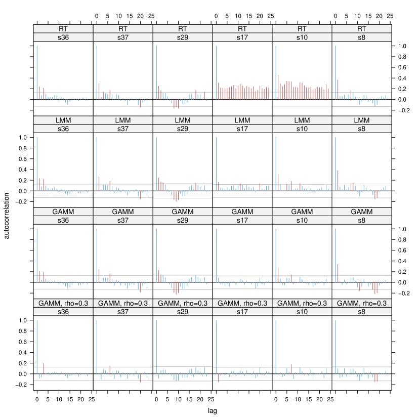
The second row of panels in Figure 1 presents the autocorrelation functions for the residuals of a linear mixed-effects model fitted to the word naming latencies with random intercepts for item (verb) and by-subject random intercepts as well as by-subject random slopes for Trial (the order number of the word in the experimental list, i.e., the variable defining the time series in this data set). Using the lme4 package (Bates et al.,, 2015) for R (version 3.0.2), the specification of the random effects ((1 + Trial|Subject)) requests by-subject random intercepts, by-subject random slopes for Trial, and a correlation parameter for the random intercepts and slopes.

naming.lmer = lmer(RT ~  Regularity + Number + Voicing + InitialNeighbors +
                   InflectionalEntropy + poly(Frequency, 2) + Trial +
                   (1 + Trial|Subject) + (1|Verb),
                   data = naming)

Figure 1 (second row) indicates that the thick autocorrelational structure for subjects 17 and 10 has been eliminated by the by-subject random regression lines, but the less prominent autocorrelational structure for the other subjects has remained virtually unchanged.

The third row of panels of Figure 1 shows that a gamm with by-subject factor smooths for Trial, replacing the by-subject straight lines of the linear mixed model yields very similar results. Using the bam function from mgcv for R, the model specification

naming.gam = bam(RT ~ Regularity + Number + Voicing + InitialNeighbors +
                 InflectionalEntropy + s(Frequency) +
                 s(Trial, Subject, bs="fs",m=1) + s(Verb, bs="re"),
                 data=naming)

requests random intercepts for the verbs (s(Verb, bs="re")) and by-subject wiggly penalized curves for Trial (s(Trial, Subject, bs="fs", m=1), here, bs="fs" requests factor smooths with the same smoothing parameters across subjects, and m=1 requests shrinkage to obtain wiggly random effects).

An improvement is obtained by including an autoregressive ar(1) process for the errors:

$$e_{t}=\rho e_{t-1}+\epsilon_{t},\hskip 10.00002pt\epsilon_{t}\sim{\cal N}(0,\sigma).$$ (1)

This equation specifies that the current error is similar to the preceding error by a factor $\rho$, with Gaussian noise added. As the current error depends only on the preceding error, this is a first-order autoregressive process. Second-order or higher autoregressive process would also take into account the error at $t-k,k=2,3,\ldots$ . The bam function in the mgcv package offers the possibility of taking a first-order autoregressive process into account by specifying the autoregressive proportionality $\rho$ (with the rho directive in the function call) and by supplying a variable in the data frame, here NewTimeSeries (with levels true, false), indicating the beginning of each new time series with the value true (here, the first trial for each subject), to be supplied to the directive AR.start in the call to bam:

naming.r.gam = bam(RT ~ Regularity + Number + Voicing + InitialNeighbors +
                     InflectionalEntropy + s(Frequency) +
                     s(Trial, Subject, bs="fs",m=1) + s(Verb, bs="re"),
                     rho=0.3, AR.start=naming$NewTimeSeries,
                     data=naming)

There is no automatic procedure for the selection of the value of $\rho$. The autocorrelation at lag 1 is a good guide for an initial guesstimate, which may need further adjusting. When changing $\rho$, it is important not to increase $\rho$ when this does not lead to a visible reduction in autocorrelation, at the cost of inflated goodness of fit and warped effects of key predictors. It should be kept in mind that an ar(1) autocorrelative process is only the simplest of possible autocorrelative processes that may be going on in the data, and that hence increasing $\rho$ beyond where it is functional can distort results. The final row of Figure 1 shows that for this example, nearly all autocorrelational structure is eliminated with a small $\rho=0.3$.

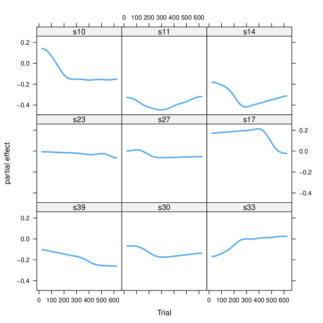
The summary of this model, shown in Table 1, shows strong support for the random effects structure for Verb and Subject, with large $t$-values and small $p$-values. Typical examples of by-subject random wiggly curves are shown in Figure 2. These curves capture both changes in intercept, as well as changes over time. For some subjects, the changes are negligible, but for others, they can be substantial, and non-linear.

Table 1: A gamm fitted to log-transformed picture naming latencies ($\rho=0.3$); s: thin plate regression spline, fs: factor smooth, re: random effect.

A. parametric coefficients	Estimate	Std. Error	t-value	p-value
Intercept	6.5531	0.0512	127.9396	$<$ 0.0001
Regularity=regular	0.0093	0.0094	0.9986	0.3180
Number=singular	-0.1147	0.0513	-2.2377	0.0253
Voicing=present	0.0269	0.0101	2.6734	0.0075
Initial Neighborhood Size	0.0179	0.0055	3.2499	0.0012
Inflectional Entropy	-0.0343	0.0159	-2.1616	0.0307
B. smooth terms	edf	Ref.df	F-value	p-value
s(word frequency)	4.2914	4.6233	7.7445	$<$ 0.0001
fs(Trial, subject)	99.4223	358.0000	5.6670	$<$ 0.0001
re(verb)	190.1753	280.0000	2.1085	$<$ 0.0001

Figure 2: Selected by-subject random wiggly curves for Trial (penalized factor smooths) in the gamm fitted to word naming latencies.

One could consider replacing the factor smooths by by-subject random intercepts, while at the same time increasing $\rho$. However, a model such as

bam(RT ~ Regularity + Number + Voicing + InitialNeighbors +
         InflectionalEntropy + s(Frequency) +
         s(Subject, bs="re") + s(Verb, bs="re"),
         rho=0.9, AR.start=naming$NewTimeSeries,
         data=naming)

provides an inferior fit with an adjusted R-squared of 0.07 (compare 0.36) and an freml score of 2655 (compare 684). This suggests that in this data set, two very different kinds of processes unfold. One of these processes is autoregressive in nature, with a relatively small $\rho$. Possibly, these autoregressive processes reflect minor fluctuations in attention. The other process may reflect higher-order cognitive processes relating to practice and fatigue, such as exemplified by the fastest subject (s11) in Figure 2, who initially improved her speed, but then, as the experiment progressed, was not able to maintain her rapid rate of responding.

Although these task effects typically are not of interest to an investigator's central research question, careful modeling of these task effects is important for the evaluation of one's hypotheses. For instance, the linear mixed effects model mentioned previously does not support an effect of inflectional entropy (Shannon's entropy calculated over the probabilities of a verb's inflectional variants) with $t=-1.87$, whereas the gamm offers more confidence in this covariate ($t=-2.16$). However, as we shall see next, predictors may also lose significance as autocorrelational structure is brought into the model.

4 Pitch contours as time series

Koesling et al., (2012) were interested in the stress patterns of English three-constituent compounds, and measured the fundamental frequency of such compounds as realized by a sample of speakers. In what follows, the response variable of this study, pitch, is measured in semitones.

As can be seen by inspecting the top panels of Figure 3, there are autocorrelations in the pitch contours that are much stronger than those observed for the naming latencies discussed above. In this figure, panels represent the autocorrelation functions for selected events, where an event is defined as an elementary time series consisting of the pitch measured at 100 moments in normalized time for the combination of a given compound and a given speaker. Whereas for the naming experiment, there are as many time series as there are subjects, the number of time series in the present phonetics study is equal to the number of unique combinations of subjects and compounds ($12\times 40=480$).

Figure 3: Autocorrelation functions for pitch (in semitones, top row) and model residuals (remaining rows) of selected events. Second row: gamm with by-participant random intercepts and random slopes for Time and by-compound random intercepts; Third row: gamm with by-participant and by-compound random wiggly curves; Fourth row: gamm with by-compound and by-participant random wiggly curves as well as a correction for ar(1) with $\rho=0.98$.

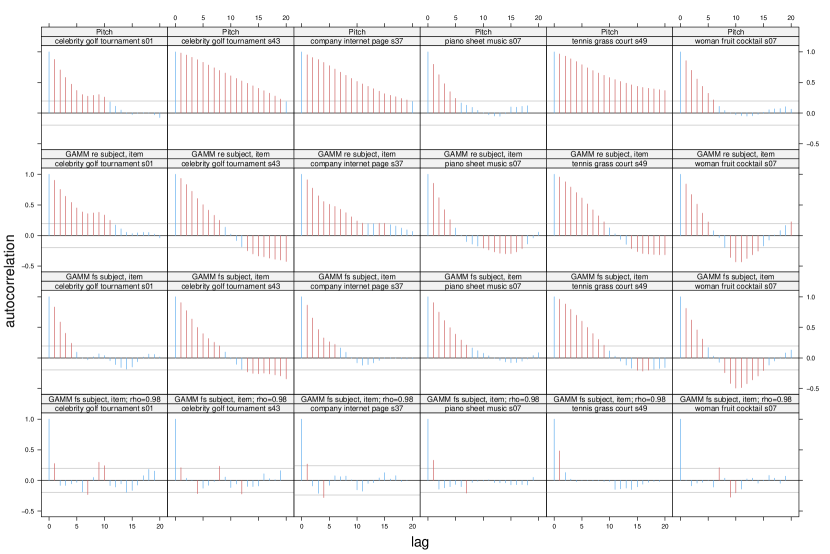
The second row of panels in Figure 3 indicates that a model with by-speaker random intercepts and slopes for (normalized) time does not succeed in consistently reducing the autoregressive structure of this data. Some improvement is achieved when by-subject and by-compound random wiggly curves are added to the model specification (third row of panels), but the errors are only whitened substantially, albeit not completely, by additionally including an autoregressive parameter $\rho=0.98$ (bottom row of panels). This fourth model was specified as follows.

pitch.gam = bam(PitchSemiTone ~ Sex + BranchingOrd +
  s(NormalizedTime) + s(NormalizedTime, by=BranchingOrd) +
  s(NormalizedTime, Speaker, bs="fs", m=1) +
  s(NormalizedTime, Compound, bs="fs", m=1) +
  s(Compound, Sex, bs="re"),
  data=pitch,
  rho=0.98, AR.start=pitch$NewTimeSeries)

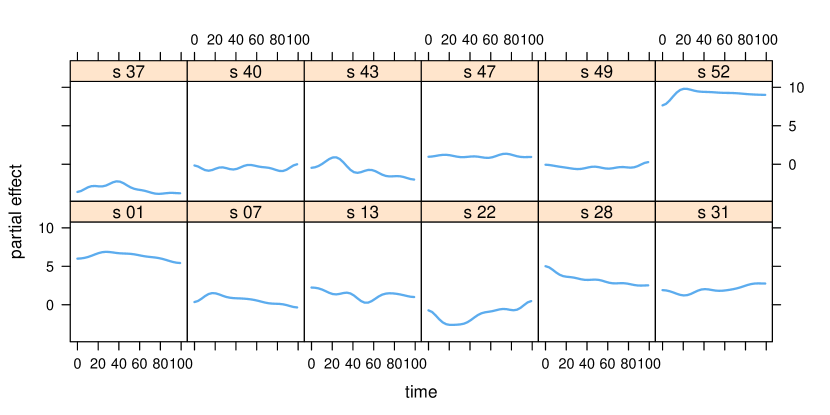
BranchingOrd is an ordered factor specifying four different compound types (defined by stress position and branching structure). The first smooth, s(NormalizedTime), specifies a wiggly curve for the reference level of this factor. The second smooth term, s(NormalizedTime, by = BranchingOrd), requests difference curves for the remaining three levels of BranchingOrd. A summary of this model is presented in Table 2. Figure 4 clarifies that the variability across speakers mainly concerns differences in the intercept (height of voice) with variation over time that is quite mild compared to the variability over time present for the compounds.

Table 2: Summary of a gamm for pitch as realized on English three-constituent compounds ($\rho=0.98$); s: thin plate regression spline, ds: difference spline, fs: factor smooth, re(compound, sex): by-compound random effects for sex.

A. parametric coefficients	Estimate	Std. Error	t-value	p-value
Intercept	91.3134	1.4594	62.5689	$<$ 0.0001
Sex = male	-13.6336	1.4649	-9.3066	$<$ 0.0001
Branching = LN2	0.7739	0.4271	1.8121	0.0700
Branching = RN2	0.2415	0.3657	0.6605	0.5089
Branching = RN3	0.6460	0.4320	1.4955	0.1348
B. smooth terms	edf	Ref.df	F-value	p-value
s(Time)	7.6892	7.9403	2.7398	0.0064
ds(Time, LN2)	6.5392	7.0804	0.6255	0.7418
ds(Time, RN2)	1.4097	1.5555	2.4744	0.1344
ds(Time, RN3)	6.4987	7.1541	1.9566	0.0411
fs(Time, speaker)	85.7092	105.0000	14.2675	$<$ 0.0001
fs(Time, compound)	248.5172	348.0000	3.5294	$<$ 0.0001
re(compound, sex)	19.0558	75.0000	0.4566	$<$ 0.0001

Figure 4: By-speaker (upper trellis) and by-compound (lower trellis) random wiggly curves in normalized time in the gamm predicting the pitch contour for English three-constituent compounds ($\rho=0.98$).

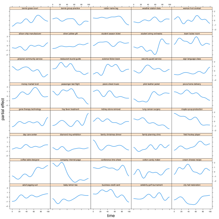
In principle, one could consider fitting a penalized factor smooth to each of the 480 individual events (time series), although this is currently computationally prohibitively expensive for the large number of events in the present study. The way the model has been specified here is optimistic in the sense that it assumes that how pitch contours are realized can be factored out into orthogonal contributions from individual subjects and from individual compounds. In a more pessimistic scenario, each event makes its own, idiosyncratic, contribution to the model's predictions. In other words, the present model seeks to capture part of the structure in the elementary time series by means of crossed wiggly curves `by subject' and `by item'.

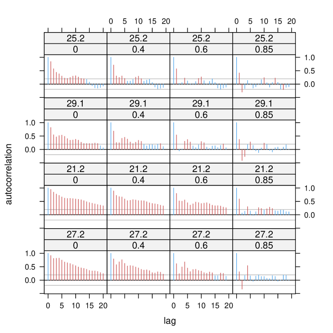
Currently, only a single autoregressive parameter $\rho$ can be specified for all events jointly. Inspection of the last row of panels of Figure 4 suggests that it is desirable to relax the assumption that $\rho$ is exactly the same for each event. Although for some events the autocorrelation function is properly flat already for a moderate $\rho$, see, e.g., the second panel on the first row ($\rho=0.4$), events remain for which autocorrelations persist across several lags.

Figure 5: Autocorrelation functions for the residuals of gamm models with $\rho=0.2,0.4,0.8,0.98$ (columns) for selected events (rows) where the largest value of $\rho$, although for most events optimal, induces artifical negative autocorrelations at some lags.

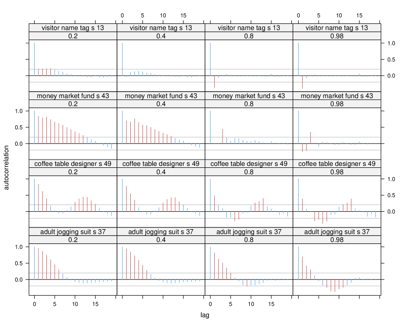
Increasing $\rho$ would remove such persistent autocorrelations, but, unfortunately, at the same time induce artificial autocorrelations for other events. This is illustrated in Figure 5, which presents, for four events (rows) the autocorrelation function for increasing values of $\rho$ (columns). For events with hardly any autocorrelation to begin with (upper panels), increasing $\rho$ artificially creates a strong negative autocorrelation at lag 1. The events in the second and third row show how increasing $\rho$ can induce artefactual autocorrelations both at shorter lags (second row) and at longer lags (third row). The event in the fourth row illustrates how increasing $\rho$ attenuates but not removes autocorrelation at shorter lags, while giving rise to new negative autocorrelation at intermediate lags.

Although higher-order autoregressive processes might be more appropriate for many events, they currently resist incorporation into gamms. Thus, the analysist is left with two strategies. The first is to select a value of $\rho$ that finds a balance between removing strong autocorrelations, while at the same time avoiding the introduction of artefactual autocorrelation for events which show little autocorrelation to begin with — inappropriate use of $\rho$ may completely obscure the actual patterns in the data.

The second strategy is to remove from the data set those events that show persistent autocorrelations for the optimal $\rho$ obtained with strategy one. When refitting the model to the remaining data points yields qualitatively similar results, it is safe to conclude that the remaining autocorrelational structure in the original model is not an issue.

Two aspects of the present model are of further interest. First, the model includes a thin plate regression smooth for the reference level of compound type (LN1), with difference smooths for the remaining three compound types. Inspection of Table 2 reveals only limited support for significant differences between the pitch contours on the four kinds of compounds, and inspection of the difference curves (in panels 2–4 in Figure 6) clarifies that there is little evidence for significant differences with the reference curve. In fact, a simpler model (not shown) with just a spline for normalized time and no main effect or interactions involving branching condition fits the data just as well.

Figure 6: The pitch contour for the LN1 branching condition, and difference curves for the remaining three branching conditions. As the confidence regions for the difference curves always contain the zero line, there is little support for differences in pitch contour as a function of branching condition.

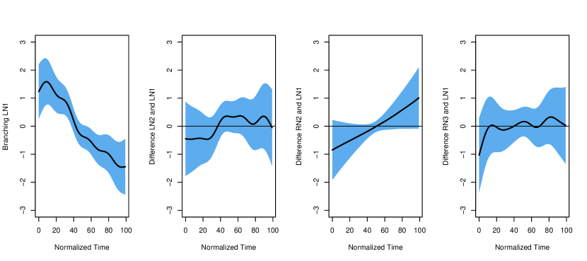
The main reason for the absence of the effect of branching condition reported originally by Koesling et al., (2012) is the inclusion of the random wiggly curves for compound. When the factor smooth for compound is replaced by random intercepts and random slopes for compound, enforcing linearity, the main effect of branching condition and its interaction with normalized time is fully significant, just as in the original study. This indicates that the variability in the realization of the pitch contours of the individual compounds is too large to support a main effect of branching condition.

We therefore remove branching condition from the model specification, and completing the model with a smooth for the frequency of occurrence of the compound,

  bam(PitchSemiTone ~ Sex + s(LogFrequency) +
                      s(NormalizedTime) +
                      s(Compound, Sex, bs="re") +
                      s(NormalizedTime, Speaker, bs="fs", m=1) +
                      s(NormalizedTime, Compound, bs="fs", m=1),
      data=pitchc,
      rho=0.98, AR.start=pitchc$NewTimeSeries)

we zoom in on the interaction of compound (random-effect factor) by sex (fixed-effect factor), specified above as s(Compound, Sex, bs="re"). Figure 7 presents a dotplot for the coefficients for the females on the horizontal axis against the coefficients for the males on the vertical axis. Words for which the males tend to raise their pitch are passenger test flight, family christmas dinner, and kidney stone removal, whereas males lower their pitch for money market fund. Females, on the other hand, lower their pitch for tennis grass court, lung cancer surgery, and passenger test flight, but raise their pitch for maple syrup production, piano sheet music, and hay fever treatment. The two sets of coefficients may even be correlated ($r=-0.31,t(38)=0.049$), such that where males substantially raise their pitch, females lower their pitch, and vice versa, possibly reflecting subtle differences in what topics the different sexes find exciting and unexciting (for pitch raising as an index of excitement, see, e.g., Paeschke et al.,, 1999; Trouvain and Barry,, 2000; Traunmüller and Eriksson,, 1995).

Figure 7: By-compound random contrasts for sex in the gamm fitted to the pitch contour of English tri-constituent compounds. Positive adjustments indicate a higher pitch.

This case study illustrates three methodological points. First, including random effect curves (by means of factor smooths) for subjects and items may lead to substantially different conclusions about the form of smooth terms in the fixed-effect part of the model specification. Just as including random slopes for a factor $X$ may render the main effect of $X$ non-significant in the context of a linear mixed-effects model, so inclusion of random wiggly curves for a time series $t$ may render an interaction s(t, by=X) non-significant. Second, the coefficients of random-effect interactions such as Compound by Sex may yield novel insights, especially in the presence of correlational structure. Third, when residuals reveal autocorrelational structure, the ar(1) parameter $\rho$ should be chosen high enough to remove substantial autocorrelational structure, but not so high that new, artificial autocorrelational structure is artefactually forced onto the data.

5 Time series in EEG registration

Similar to the pitch data, eeg data comprise many small time series, one for each event for which a subject's electrophysiological response to a particular stimulus is recorded. DeCat et al., (2014, 2015) used English compounds as stimuli, presented in their grammatical order (coal dust) and in a manipulated, reversed and ungrammatical order (dust coal) to native speakers of English as well as advanced Spanish and German learners of English. The goal of this study was to clarify whether proficiency and language background would be reflected in different electrophysiological processing signatures for these compounds. For the purposes of the present study, the specification of the random-effects structure and the measures taken to bring autocorrelational structure in the residuals under control, and the effects of the choice of $\rho$ on the fixed-effect predictors and covariates in the model are of particular interest. In what follows, the analysis is restricted to the subset of native speakers of English, and to the eeg at channel C1.

The model for these data,

eeg.gam = bam(Amplitude ~
  s(Time, k=10) + s(Time, by=ConstituentOrder, k=10) +
  te(LogFreqC1, LogFreqC2, k=4) +
  te(LogFreqC1, LogFreqC2, by=ConstituentOrder, k=4) +
  s(LogCompFreq, k=4) + s(LogCompFreq, by=ConstituentOrder, k=4) +
  s(Compound, bs="re")+
  s(Trial, Subject, bs="fs", m=1)+
  s(Time, Subject, bs="fs", m=1),
  data=eegC1, family="scat",
  AR.start=Start, rho=0.85)

comprises a smooth for time for the compounds presented with their constituents in the normal order (e.g., goldfish), and a difference curve for the condition in which constituent order is reversed (fishgold). The model furthermore takes an interaction of the constituent frequencies into account by means of a tensor product smooth, as well as the corresponding difference surface for the reversed order condition. In the light of the very large number of observations (207,600), we slightly lowered the upper bound of the number of basis functions in a given dimension to $k=4$, in order to avoid fitting overly wiggly surfaces. A thin plate regression spline is introduced to account for the effect of compound frequency, again allowing for a difference between the standard and reversed word order. Random intercepts for compound, and two by-subject factor smooths, one for Time and one for the sequence of trials in the experiment (Trial, complete the model description. The model summary is given by Table 3.

Table 3: Generalized additive mixed model fitted to the electrophysiological response of the brain at channel C1 to compound stimuli. Rev: reversed constituent order in the compound, Norm: normal order. s: thin plate regression spline, te: tensor product smooth, re: random intercepts, fs: factor smooth. ($\rho=0.85$)

A. parametric coefficients	Estimate	Std. Error	t-value	p-value
(Intercept)	0.0552	0.4221	0.1308	0.8960
B. smooth terms	edf	Ref.df	F-value	p-value
s(Time)	8.5653	8.6645	14.6953	$<$ 0.0001
s(Time):Order=reversed	1.5768	1.9624	0.9999	0.4139
s(CompFreq)	1.7242	1.7703	0.7804	0.3172
s(CompFreq):Order=reversed	2.6384	2.8746	21.1108	$<$ 0.0001
te(FreqC1,FreqC2)	6.5652	6.6936	4.4840	0.0032
te(FreqC1,FreqC2):Order=reversed	9.6440	10.5906	10.9593	$<$ 0.0001
re(Compound)	99.1995	112.0000	10.1991	$<$ 0.0001
fs(Trial,Subject)	49.5668	89.0000	12.6940	$<$ 0.0001
fs(Time,Subject)	67.4796	89.0000	8.5343	$<$ 0.0001

The contributions of the by-subject factor smooths to the model fit is presented in Figure 8. The grey dots represent the by-subject average amplitude for each of the points in time $t=4,8,12,\ldots$ milliseconds. The red line shows the average of the model fit for the same points in time. The blue lines visualize the by-subject factor smooths for Trial. Comparing the red and blue lines, it is clear that a substantial part of the wiggliness of the model fit is contributed by the factor smooths. This figure also illustrates the limitations of the factor smooths: When trends are spiky, as for instance for subjects s5 ad s6 early in time, a strongly penalized smooth will not be able to fit the data points in the spike.

Figure 8: The by-subject factor smooths for Time in the gamm fitted to the eeg data. Dots represent average response times, the red lines represent the corresponding average for the model fit, and the blue lines the individual factor smooths.

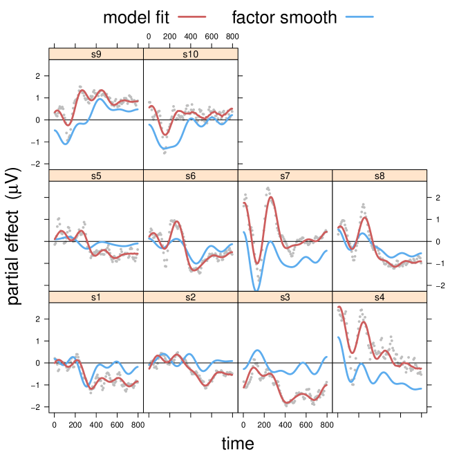
Figure 9 illustrates, for four events, that $\rho$ cannot be extended much beyond 0.85 without introducing artefactual negative autocorrelations. Interestingly, changing $\rho$ may have consequences for the predictors of theoretical interest. Figure 10 illustrates this point for four smooths in the model. The top panels show that by increasing $\rho$, the effect of word frequency, which at first blush appears to be nonlinear, becomes a straightforward linear effect. The second row of panels clarifies that the difference curve for Time, contrasting the reversed word-order condition with the normal order, is not trustworthy (see also Table 3). The increase in the 95% confidence interval that is a consequence of increasing $\rho$ to 0.85, which is required to remove the thick autocorrelative structure in the residuals (Figure 9, left columns), is noteworthy.

Figure 9: Autocorrelation functions for the residuals of gamms fitted to the amplitude of the eeg response to visually presented compounds, for four events (rows), for $\rho=0,0.4,0.6,0.85$ (columns).

The third and fourth rows of Figure 10 illustrate that the regression surface for the frequencies of the compound's constituents depends on constituent order (a threeway interaction of the frequency of the first constituent, the frequency of the second constituent, and constituent order). The contour plots in the third row show the combined effect of the constituent frequencies for the normal constituent order, modeled with a tensor product smooth. Amplitudes are greater along most of the main diagonal, suggesting qualitative differences in lexical processing for similar versus dissimilar constituent frequencies. For the normal constituent order, this surface is hardly affected by increasing $\rho$. This does not hold for the corresponding difference surface, as can be seen in the bottom row of Figure 10. In the presence of strong autocorrelations, autocorrelative noise is incorporated into the tensor surface, leading to overaccentuated and uninterpretable patterns in the lower right corner of the partial effect plots. It is only for $\rho=0.9$ that these irregularities disappear, to give way to a more interpretable difference surface: Amplitudes in the reversed order condition are reduced compared to the normal constituent order when both constituents are of a high frequency, whereas amplitudes increase when both frequencies are low. Thus, this difference surface suggests that the effect of the constituent frequencies in the normal order is largely absent when constituent order is reversed.

Figure 10: The consequences of increasing $\rho$ from 0 to 0.9 (columns) for the effect of frequency (top), the difference curve for Time contrasting the reversed constituent order with the normal order, the interaction of the frequencies of the first and second constituents (third row), and the difference surface for these predictors contrasting the reversed with the normal constituent order (fourth row).

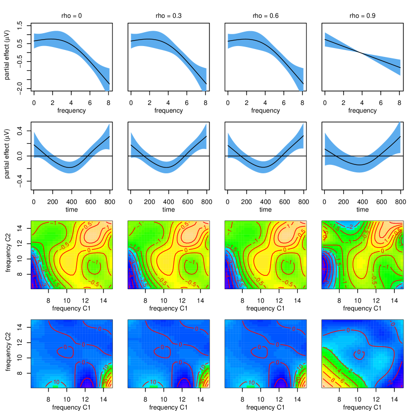
In summary, removal of autocorrelative structure in the residuals by means of the $\rho$ parameter for an ar(1) error process may have two important consequences. First of all, analyses will tend to become more conservative. Second, the functional form of nonlinear partial effects may change. In the present examples, excess wiggliness is removed.

6 Concluding remarks

This study illustrates with three examples the potential of generalized additive mixed models for the analysis of language data: response latencies for reading aloud, pitch contours of three-constituent compounds, and the electrophysiological response of the brain to grammatical and ungrammatical compounds.

Gamms provide the analyst with two tools for coming to grips with autocorrelational structure in the model residuals: factor smooths and the ar(1) $\rho$ parameter. In the standard linear mixed effects model, systematic changes in how a subject performs over the course of an experiment, or during an experimental trial with a time-series structure, can only be accounted for by means of random intercepts and random slopes. Factor smooths relax this assumption of linearity, and thereby have the potential to provide much tighter fits when random-effect factors indeed behave in a non-linear way.

Autocorrelational structure in the errors may, however, remain even after inclusion of factor smooths. For the reaction times revisited in this study, most of the autocorrelational structure was accounted for by means of factor smooths for the time series constituted by a participant's responses over the time course of the experiment. A mild value of the ar(1) correlation parameter ($\rho=0.3$) was sufficient to further whiten the residuals. For the pitch data, and the same holds for the eeg data, inclusion of by-participant and by-item factor smooths was not successful at all for removing the autocorrelation. Here, a high value for the ar(1) correlation parameter was necessary for approximate whitening of the errors.

Whitening the errors is important for two reasons (see also Baayen et al.,, 2015, for further discussion). First, it protects the analyst against anti-conservative p-values. Second, models with whitened errors are more likely to provide an accurate window on the quantitative structure of the data. The analysis of pitch contours provided an example of the inclusion of a factor smooth rendering a time by fixed-factor interaction non-significant. Furthermore, whitening ar(1) errors may change the functional form of the effect of predictors of interest. The analysis of the eeg data illustrated how an effect that initially seemed nonlinear became straightforwardly linear, as well as a non-linear regression surface that became simplified and better interpretable thanks to whitening.

References

- Baayen et al., (2015) Baayen, R., Vasishth, S., Bates, D., and Kliegl, R. (2015). Out of the cage of shadows. arxiv.org, http://arxiv.org/abs/1511.03120.
- Baayen, (2013) Baayen, R. H. (2013). Multivariate Statistics. In Podesva, R. and Sharma, D., editors, Research Methods in Linguistics, pages 337–372. Cambridge University Press, Cambridge.
- Baayen and Milin, (2010) Baayen, R. H. and Milin, P. (2010). Analyzing reaction times. International Journal of Psychological Research, 3:12–28.
- Bates et al., (2015) Bates, D., Mächler, M., Bolker, B., and Walker, S. (2015). Fitting linear mixed-effects models using lme4. Journal of Statistical Software, 67(1):1–48.
- Broadbent, (1971) Broadbent, D. (1971). Decision and Stress. Accademic Press, New York.
- De Vaan et al., (2007) De Vaan, L., Schreuder, R., and Baayen, R. H. (2007). Regular morphologically complex neologisms leave detectable traces in the mental lexicon. The Mental Lexicon, 2:1–23.
- DeCat et al., (2014) DeCat, C., Baayen, R. H., and Klepousniotou, E. (2014). Electrophysiological correlates of noun-noun compound processing by non-native speakers of english. In Proceedings of the First Workshop on Computational Approaches to Compound Analysis (ComAComA 2014), pages 41–52, Dublin, Ireland. Association for Computational Linguistics and Dublin City University.
- DeCat et al., (2015) DeCat, C., Klepousniotou, E., and Baayen, R. H. (2015). Representational deficit or processing effect? a neuro-psychological study of noun-noun compound processing by very advanced l2 speakers of english. Frontiers in Psychology (Language Sciences), 6:77.
- Koesling et al., (2012) Koesling, K., Kunter, G., Baayen, R. H., and Plag, I. (2012). Prominence in triconstituent compounds: Pitch contours and linguistic theory. Language and Speech, 56(4):529–554.
- Lin and Zhang, (1999) Lin, X. and Zhang, D. (1999). Inference in generalized additive mixed models using smoothing splines. JRSSB, 61:381–400.
- Paeschke et al., (1999) Paeschke, A., Kienast, M., and Sendlmeier, W. (1999). F0-contours in emotional speech. In Proc. 14th Int. Congress of Phonetic Sciences, volume 2, pages 929–932.
- Sanders, (1998) Sanders, A. (1998). Elements of Human Performance: Reaction Processes and Attention in Human Skill. Lawrence Erlbaum, Mahwah, New Jersey.
- Tabak, (2010) Tabak, W. (2010). Semantics and (Ir)regular Inflection in Morphological Processing. Ponsen & Looijen, Ede. PhD thesis, University of Nijmegen.
- Taylor and Lupker, (2001) Taylor, T. E. and Lupker, S. J. (2001). Sequential effects in naming: A time-criterion account. Journal of Experimental Psychology: Learning, Memory and Cognition, 27:117–138.
- Traunmüller and Eriksson, (1995) Traunmüller, H. and Eriksson, A. (1995). The frequency range of the voice fundamental in the speech of male and female adults. Unpublished manuscript, Institutionen för lingvistik, Stockholms universitet, S-106 91 Stockholm, Sweden.
- Trouvain and Barry, (2000) Trouvain, J. and Barry, W. J. (2000). The prosody of excitement in horse race commentaries. In ISCA Tutorial and Research Workshop (ITRW) on Speech and Emotion.
- Welford, (1980) Welford, A. (1980). Choice reaction time: Basic concepts. In Welford, A., editor, Reaction Times, pages 73–128. Accademic Press, New York.
- Wilkinson and Rogers, (1973) Wilkinson, G. and Rogers, C. (1973). Symbolic description of factorial models for analysis of variance. Applied Statistics, pages 392–399.
- Wood, (2006) Wood, S. N. (2006). Generalized Additive Models. Chapman & Hall/CRC, New York.
- Wood, (2011) Wood, S. N. (2011). Fast stable restricted maximum likelihood and marginal likelihood estimation of semiparametric generalized linear models. Journal of the Royal Statistical Society (B), 73:3–36.
- Wood, (2013) Wood, S. N. (2013). On p-values for smooth components of an extended generalized additive model. Biometrika, 100:221–228.