Abstract

The model by Nieves, Ruiz-Simo, Vicente Vacas, and their group (IFIC, Valencia, Spain) for 2p2h reactions that produce QE-like (no pion) final states has been implemented in GENIE. Since the model currently does not predict the kinematics of the outgoing hadrons, a simple two-nucleon system is grafted onto the model’s prediction of isospin, energy transfer, and momentum transfer. These two nucleons are then given to the GENIE FSI models. This technical note is a guide to the kind of information available from this model and some limitations. There are several figures that illustrate the output of the model, and detailed discussion of the physics context for this model. Finally, any other authors’ model (or variations of this one) that can be expressed as hadronic tensors for total and pn initial state will be easy to incorporate into this framework, or possibly be made available as a reweight to events generated with this model. The 2017 version of this document is updated to reflect the as-released GENIE 2.12.6 version of the code, which produces identical results to the development versions.

1 Introduction

This technical note describes the initial GENIE implementation of the Valencia group’s model for QE-like two-particle, two-hole (2p2h) (or meson exchange current MEC) reactions. This is one effort in a longstanding campaign by members of the Instituto de Fisica Corpuscular (IFIC) to describe neutrino nucleus reactions. Now available in GENIE, their work is available for wider use. We will refer to these as “IFIC Valencia model”. It is sometimes referred to as the Nieves model or the Valencia model, and the primary authors are Nieves, Ruiz Simo, and Vicente Vacas with contributions from Oset and Alvarez Ruso at IFIC. The model is described in references [1, 2]. This implementation incorporates a kinematic cutoff at 1.2 GeV of momentum transfer, described in the latter reference, allowing it to be used at higher energies.

With a QE model that importantly includes the RPA effect and a local Fermi-gas [3], the combination describes MiniBooNE QE-like p_μ, $\theta_{\mu}$ data [4] and MINERvA QE-like $Q^{2}$ cross section shape [2] better than either experiments’ default QE and Delta background models. This implementation, available as of version 2.12.6 of GENIE, was used (in the form of a back-ported private build of version 2.8.4) for the comparisons in [5] and later MINERvA papers, for which the present paper serves as a technical reference. When combined with updated deuterium form factor constraints such as [6] and uncertainties on the RPA effect [7] for example, these elements can replace the anomalously high axial mass and its uncertainty. This enables the community to proceed with precision measurements of these processes.

The cross section calculation is fast because the hadronic tensor is pre-computed and available in tabulated form. Essentially all the physics is related to the energy and momentum transfer from the lepton to the nucleus. These tensor tables serve for all energies, for neutrino and anti-neutrino, and all lepton flavors. It is contracted with the leptonic tensor, a fast calculation with no integrations, which account for the lepton mass and energy. That this would be a productive implementation originated with Federico Sanchez as part of work on the [2] paper; Sanchez also wrote the first C++ skeleton code that calls the model authors’ FORTRAN routines. The GENIE code is a combination of this skeleton and the previous MEC model in GENIE.

There is a tensor table each for the full cross section for three nuclei, ¹²C, ¹⁶O, and ⁴⁰Ca from the original references [4, 2], plus four additional nuclei. These are enough to cover the rest of the periodic table with a nucleon combinatorics scaling, described in Sec. 6. Additional hadronic tensor tables provide the cross section for scattering on pn initial nucleon states, which are used internally to generate the isospin final states according to the model. Two more tensor tables for each nuclei are provided for a $\Delta$-only version of the full and pn cross section; the physics of this component is discussed in Sec. 5, and may be especially useful for systematics studies.

The hadron tensor part of the technique described here is not specific to these authors’ model. Other model authors’ work, or future variations on the IFIC model, can be dropped into GENIE simply by providing a revised hadronic tensor. For example, the earliest full calculation of a neutrino-carbon 2p2h model was done by Martini and Ericson [8] and could be available within GENIE using this same codebase. The technique may even be useful to make fast comparisons of different author’s QE process. Some comments on this are available in a later section.

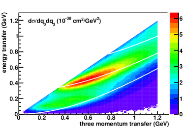
Mosts figures in this document are done with pre-release version and GENIE 2.8 and 2.10 and all default settings. The results are the same when obtained from the released version GENIE 2.12.6 . The hadronic tensors used are from the original author’s version HP4.2 which was used for most of the 2013-era paper [2]. We are using a notation in this document where $q_{0}$ is the energy transfer, sometimes called $\omega$ or $\nu$, and $q_{3}$ is the magnitude of the three-momentum transfer, also naturally called $|\vec{p}|$ or sometimes just $p$. These are the components of a four vector such that $-q^{2}=Q^{2}=q_{3}^{2}-q_{0}^{2}$ is the invariant square of the four-momentum transfer.

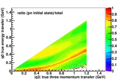
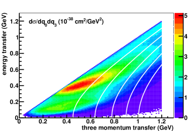
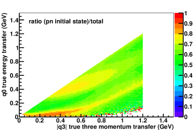
Cross sections are often calculated for muon kinematics p_μ and $\theta_{\mu}$ in the lab/nucleus rest frame. Here we present it in the energy and momentum transfer quantities. Figure 1 shows the cross section overlaid with lines of constant W = 0.938, 1.232, and 1.535 GeV. The resulting QE-like 2p2h differential cross section has two components, a $\Delta$(1232)-like component and a dip-region component just above W=0.938 GeV. The lower plots are the anti-neutrino cross section, but with lines of constant $Q^{2}$. The cross section shown is obtained from 3 GeV neutrinos by generating millions of events on carbon nuclei, binning them, and scaling by the total $\sigma$ captured from the model available in the GENIE spline value. The right plots are the model’s prediction for the fraction of events that had pn initial states, which will be pp final states in the neutrino case (top) and nn final states for anti-neutrinos (bottom). This is the essential information available from the model. These predictions change only slightly switching from muon to the lighter electron.

Figure 1: The differential cross section from the GENIE implementation of the QE-like 2p2h model (right) and the fraction of the total cross section with a pn initial state (left). The top plots are $\nu$C while the lower plots are $\bar{\nu}$C, both at 3 GeV. To guide the eye in this kinematics space, the neutrino figure has lines of constant W = 938, 1232, 1520 MeV emphasizing the dip region, and the anti-neutrino figure has lines of constant $Q^{2}$ from 0.2 to 1.0 GeV² emphasizing the low $Q^{2}$ nature of the cross section.

After the lepton kinematics are chosen for each generated event, the GENIE implementation grafts a hadron system final state. This discards some correlation of the cross section with the initial nucleon system, and simplifies how the two nucleons share the energy and momentum transfer. The full calculation is not available in a hadronic tensor style implementation, because the detailed hadron kinematics are hidden in the inner integrations of the model, so this is the best we can do. This initial implementation, combined with data from recent experiments, may promote future work on the details of the model. This hadron methodology is similar in design to what is implemented [9] in NuWro and in the phenomenological MEC model in GENIE authored by Steve Dytman. This simple method appears to be a good approximation [10] to the proton angles from a full calculation.

A beneficial consequence of building the hadron state independent from (except $q_{0}$,$q_{3}$) the lepton state is that an event generated with the IFIC Valencia model in GENIE is necessarily the same as would be generated from an alternate model which only provides $d^{2}\sigma/dq_{0}q_{3}$ and not correlated hadron information. That permits opportunities to reweight events generated with one model to be identical to a variation of (or another author’s) model for $d^{2}\sigma/dq_{0}q_{3}$. For the same reason, it is possible to reweight a quasi-elastic model to another $d^{2}\sigma/dq_{0}q_{3}$, an approximation that misses only some correlation expected between the initial and final nucleon state that may be present in one model or the other. Especially when the final nucleon states are further modified by rescattering as they exit the nucleus, the correlations may anyway be challenging to observe. This strategy is widely exploited by the experimental community to make fast comparisons or fitting or rapid evaluation of systematic uncertainties.

This paper outlines the basic procedural steps in the next section. After that are a series of subsections that touch on specific outcomes of this implementation, especially the resulting hadronic systems and where they might diverge from the model author’s calculations. Practical and optimization concerns mean that the resulting cross section will not be identical to the original calculation. However all results are benchmarked against the original code, and the design goal is to reproduce that with 2% accuracy in the cross section lepton kinematics. For a prediction, this seems a good match for testing against current and imminent data sets.

2 Basic procedure

• Use accept-reject method in $p_{\mu}$, $\theta_{\mu}$ to draw momentum and energy transfer kinematics up to 1.2 GeV according to the IFIC Valencia model.

• Assign the energy and momentum transfer to a pair of nucleons drawn from the user’s favorite nucleon momentum distribution.

• “Decay” that nucleon cluster back-to-back and isotropically to two nucleons in the center of momentum frame and boost back to the lab frame.

• the two nucleons are available to be rescattered by the user’s favorite final state interaction model.

The accept-reject method is seeded with a maximum cross section to improve generation efficiency. Even though the cross section is approximately the same as a function of $q_{0}$ and $q_{3}$, the method is applied in the not-invariant kinematics $p_{\mu}$ and $\theta_{\mu}$. This means that the maximum double-differential cross section for any muon kinematics increases with energy. A simple but safe log-log parameterization was created once and hard-coded, then used to compute a maximum cross section. (This technical issue could be replaced by a fast lookup of a cached value.) This maximum value is scaled away from A=12 by a generous function A^1.4 because some components may increases faster with A. These are specific to IFIC model, using Martini’s model will require different constants. This does not change the physics of the model, just allows more efficient generation of events.

Are the initial two nucleons pn or not ? This is drawn from the cross section also. The hadron tensor computed for the entire cross section was used when the kinematics were chosen. A second cross section is computed for these same kinematics for the pn initial state only. The ratio of the pn cross section is taken with the total cross section. Then a random number is compared to that ratio to decide whether the pn initial state is chosen.

The initial nucleon pair is drawn from the prevailing GENIE Fermi momentum distribution. For Genie 2.12 and and earlier it is a Fermi gas with the Bodek-Ritchie high momentum tail. The four-momentum sum of the nucleons is computed and saved to the GHEP record as a nucleon cluster. In this implementation, the original momentum of each nucleon is forgotten. If the user chooses a non-default Fermi momentum distribution, that will be used.

The momentum and energy transfer, plus one unit charge, is given to the nucleon pair. If the resulting nucleon pair would be off shell, then we loop and rethrow for another nucleon pair.

The nucleon pair is then “decayed” using a CERNLIB era phase space decayer available through ROOT. Again, this process knows nothing about the initial momenta of the nucleons, only the total four-momentum of the system. The “decay” is back to back and isotropic in the center of momentum system, and is then boosted back to the lab/nucleus rest frame.

The resulting nucleons are available to be rescattered using the prevailing FSI model in GENIE. There is a very high probability of at least a soft, elastic scatter, and better than 50% chance that three or more nucleons will exist the nucleus.

The code also has a method which will return the integrated cross section, for making splines and other uses. It is simply a numerical integration of the cross section computed in $q_{0}$,$q_{3}$ kinematic space. The GENIE procedure is to produce a spline with some points that span an energy range logarithmically, then use a cubic spline interpolation to get a specific energy within the tabulated points. For the 3 GeV neutrino - carbon reaction, it returns 1.4643 x 10^-38 cm², with 1.0943 x 10^-38 cm² for anti-neutrino . A high resolution integration directly from the model yields 1.4621 x 10^-38, which is the same.

The cross sections for electron neutrino interactions are slightly higher, because the lower lepton mass opens up slightly more phase space. It especially appears along the line of maximum $q_{0}$ and $q_{3}$, all of which is kinematically at $Q^{2}\sim 0$ GeV². It is 1.3% different at 3 GeV (1.5% for anti-neutrinos), and about 6% higher at 1 GeV (7% different for anti-neutrinos) compared to the prediction for muon neutrinos.

Figure 2: The $\sigma(E)$ cross section from the GENIE implementation of the QE-like 2p2h model, including the kinematic cutoff $q_{3}<1.2$ GeV. This is the neutrino (black) and anti-neutrino (green) spline.

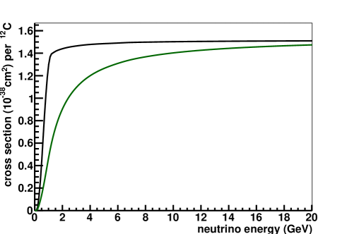
A plot of the nu-C (black) and nubar-C (green) $\sigma(E)$ splines generated by GENIE are shown in Fig. 2. The sharp behavior in the neutrino case happens as the neutrino energy drops below 1.2 GeV and eats into the limited kinematic space of this version of the model. The anti-neutrino case has a slower turn-on of the cross section because of the axial interference term. Both these characteristics follow the familiar trends of the QE cross section.

Q2 and Enu distributions

Traditionally, the QE and resonance region have been described using the invariant square of the four-momentum transfer $Q^{2}$. Analyzing data using only lepton kinematics (and QE hypothesis) causes biased energy and $Q^{2}$ estimators for the fraction of QE-like non-QE reactions from resonances and 2p2h processes. Illustration of these effects, generated from these samples, are shown in Fig. 3.

Figure 3: The model’s $Q^{2}$ distribution (flatter), and one with the QE hypothesis (more peaked at zero) on the left show the effect of using only the muon kinematics to reconstruct these events. Also shown is the $E_{\nu}$ distribution with the QE hypothesis on the right, for 3 GeV incident neutrinos.

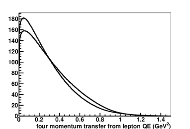
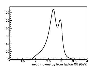
These events are predicted to be intrinsically very low $Q^{2}$, and especially so when reconstructed using the QE hypothesis. The published $Q^{2}$ distributions and differential cross sections from data all want fewer low-$Q^{2}$ interactions. Compared to that, the addition of this process would seem to worsen the agreement of the data and a simple Fermi-gas model. However, there is a similar but opposite story with adding RPA effects to the QE process, which reduces the predicted event rate at very low $Q^{2}$ more than this MEC process adds it. The combination of the two improve agreement with the data in ways that neither alone can accomplish, see for example [2] and especially [5]. Variations of the QE process with RPA are available from several calculations and if necessary can be implemented as a $q_{0}$, $q_{3}$ or $Q^{2}$ reweight [7].

Another concern is how the QE hypothesis is used when determining the energy reconstruction. These effects have long been known (e.g. [11]) to bias reconstructed kinematics of the $\Delta$ process, but many authors are pointing it out anew [12, 13, 14] and quantifying the distortions of precision neutrino oscillation spectra for the MEC process. This is more important for Cerenkov detectors than for calorimetric detectors, and is most critical when the model is missing a non-QE process completely. For particles which are further “above the QE line” in W or $q_{0}$, the QE hypothesis causes the incident neutrino energy to be systematically underestimated. Because the neutrino energy estimate is used to compute $Q^{2}$, it too is underestimated. The left most peak in the right plot of Fig. 3 is primarily from the Delta-like events. Like 1p1h Delta events, if they were reconstructed with the QE hypothesis, the 3 GeV events would have their energy estimated about 10% low. The peak near 3 GeV is from the band that keeps closest to the QE line. They are also biased low, but not as much.

Selected kinematics saved in the GENIE record

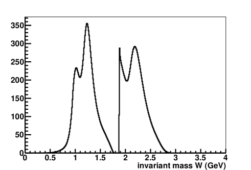
GENIE allows a model to save what “selected kinematics” were used at the vertex. This implementation sets the inelasticity y = $q_{0}$/$E_{\nu}$ and $Q^{2}$ = $q_{3}^{2}-q_{0}^{2}$, the final state lepton four vector, and the hadron (two-nucleon) combined four-vector after the reaction. We put in the hadron invariant mass W also, built from the two nucleons that we put in the nucleus, though its not especially interesting, nor is it accurate that the model really selected it. The selected t and Bjorken x variables that GENIE is willing to save are not used.

More interesting is the effective “experimenter’s W”, which assumes a single nucleon $W^{2}=M_{n}^{2}+2M_{n}q_{0}-Q^{2}$, which the user can calculate later from either true or reconstructed quantities. The proper two-nucleon W and the experimenter’s W are both shown in Fig. 4. In each there are two peaks, the right-most peak is the Delta-like component, and the left-most peak is the more proper “dip region” component.

Figure 4: The two W distributions. The right distribution is the actual W with two nucleons, before FSI. The left distribution is the single-nucleon “experimenter’s W”. The dip-region 2p2h population appears near W = 1.0 GeV in the latter, higher than QE events.

3 Hadron kinematics distributions

We emphasize the implementation of the simplest hadron system and report what it produces. How many nucleons are in the final state and what fraction goes to protons are good observables for experiments that can do tracking and/or calorimetry. All the distributions below are with FSI, of course. Unlocking the information contained in the model might reveal different energy sharing or angle dependence of the resulting nucleons. At this time we have not devised a way to provide an uncertainty on this detail of the model; that may come with some operational experience.

3.1 nucleon multiplicity

The interaction produces two nucleons specifically, and for $\nu$-C, it prefers pp final states. Even after intranuclear rescattering, it almost never happens that there are zero protons (blue line), and the number of neutrons is always less (red line), as shown in Fig. 5. The total nucleon multiplicity is shown in black and starts at two nucleons as expected. With reinteractions via the GENIE FSI model, over half the events have three or more nucleons in the final state. The probability for nucleon FSI was already high, and there are two nucleons making their way out of the nucleus in this case. The proton, neutron trends trade places for anti-neutrino reactions, and the post-FSI GENIE final state will frequently have no protons in it.

Figure 5: Number of nucleons (black), protons (blue) and neutrons (red) produced from two nucleons but after FSI. For 3.0 GeV neutrinos interacting in carbon-12 (left) and calcium-40 (right)

3.2 energy sharing

The plot on the left in Fig. 6 illustrates how the nucleon energy is shared after the isotropic decay is boosted to the lab frame and FSI is run. The plot on the right is specifically for the most energetic two protons. Each figure has three lines representing the different momentum transfer regions. The nucleons are sorted by kinetic energy, and the horizontal axis is how much fractionally is the second nucleon’s KE is compared to the first. The distribution depends on how much boost the initial nucleon pair had and so how asymmetric the products could be.

Figure 6: Energy sharing fraction (KE second nucleon)/(KE leading nucleon). The left plot is for any of pp, pn, or nn, the right plot is for the most energetic two protons only. Blue is $q_{3}<0.4$, black is $0.4<q_{3}<0.8$ and red is $0.8<q_{3}<1.2$ GeV sub samples.

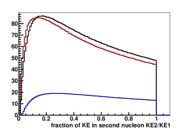
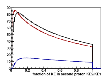
At low $q_{3}$, the energy sharing (after the boost back to the lab frame and after FSI) spans the whole range of possibilities. There is a good probability that the two nucleons are sharing the energy equally, and since they are low energy, neither travels very far. In a coarse grained scintillator detector, they may deposit signals in only one channel. There are higher energy transfers available at higher $q_{3}$, producing nucleons that are much more asymmetric.

3.3 available energy and missing energy

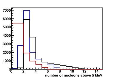
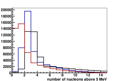
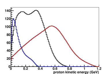
The plots in Fig. 7 illustrate different aspects of the energy in the hadron system, as might be viewed by a calorimetric or fine-grained tracking detector. The left figure shows how much energy will be easily seen in the detector as protons that can be tracked and/or analyzed calorimeterically. The black curve shows two peaks which are a combination of the pn and pp final states as well as the $\Delta$ and non-$\Delta$ contributions to the cross section.

Figure 7: The available (i.e. sum the proton KE, but not the neutrons) energy on the left, for q3 $<$ 0.4 (blue), 0.4 $<$ q3 $<$ 0.8 (black), and 0.8 $<$ q3 $<$ 1.2 GeV (red). On the right is the missing energy, lost to unbinding nucleons in the interaction (with the sharp cutoff at 0.05 GeV) and later during FSI (with a longer missing energy tail).

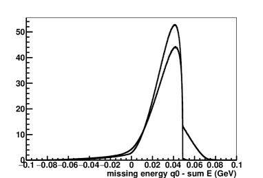
The plot on the right in Fig. 7 shows the difference between the energy transfer and the sum of the energy of the particles that exit the reaction. The dominant feature is the peak at 50 MeV, corresponding to the two units of nucleon removal energy. The curve with the sharp cutoff is before FSI, and broadened one is after FSI. Both curves have another tail on the negative side corresponding to extra energy, which I think comes from striking nucleons with unusually high momentum.

4 More Technical Details

4.1 Hadron tensor interpolation

The hadron tensors are read into Genie’s BLI2DNonUnifGrid class, whose Evaluate() method does a bilinear interpolation. The original IFIC Valencia model code also does a bilinear interpolation. The bilinear interpolation algorithm applied to the tabular hadronic tensor is different than the one the original authors used; it interpolates beyond the first entries in the table, as if there is an entry beyond that with a value of zero. This leads to slight differences in the resulting cross section. But the interpolation method is separate from the physics of the process, so we have allowed that difference to remain. Another suggestion from the original authors is to use a 2D spline instead of bilinear interpolation, though it seems unnecessary to achieve the 1% accuracy.

4.2 Hadron tensor resolution effects

The hadronic tensor can be made with different step sizes. Historically, Nieves and Vicente’s code produces it with 120 steps between 0 and 1.2 GeV in q0 and q3, which is used in this implementation also. The resulting tensor requires two days on a 2014-era 4-core machine using MPI. Gran generated a tensor with 240 steps between 0 and 1.2 GeV, so four times the number of data points, which requires about eight days. These tests use the same interpolation code, just different input tensors.

Figure 8: Effect of switching from a 240x240 HadTensor to a 120x120 HadTensor. The top shows the color axis with a $\pm$5% range, the bottom shows it with a $\pm$2% range. The artifact at the top right is basically right at 5%. [Flatten these figures to reduce the filesize…]

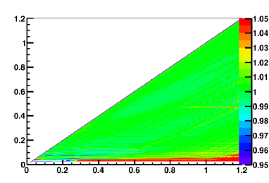
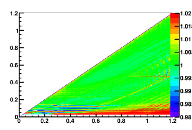
Differences appear at the 2% to 5% level, and none follow the main lines of high cross section. These tests use the same interpolation code, once the hadronic tensor is read in. It is not clear whether the few percent wiggles, or the horizontal artifact just below $q_{0}$ of 0.5 GeV is a problem or failure in one or the other calculations. It might simply be riding the numerical precision of the underlying cross section integrations.

The differences start to appear as you go lower and lower in neutrino energy, producing a $\sigma(E)$ that is 1% different or worse as you go below 250 MeV neutrino energy. Since the differences are small, it makes sense to use the smaller files. What is potentially a more interesting use of CPU power is to increase the steps and precision in some of the inner integrations and watch for effects at high $q_{3}$.

4.3 Hadron tensor as text file

The hadron tensor is provided as a plain text file containing 5 x 120 x 120 double-precision numbers. For GENIE, we have reduced the file size by truncating the FORTRAN output text precision to five significant figures and representing zero with a single digit using a python text processing script provided by Phil Rodrigues. This step reduces the file size by a factor of five. When tested, the resulting distributions are within 0.5% everywhere which had statistics good enough to tell, so this is as expected.

Another choice would be to save the HadTensor as a binary file, either of 8-byte (or even 4-byte) numbers, which might be rapidly read in, and be similar or smaller in size. Not sure this is relevant.

The text files could also be distributed as a tar.gz or tar.bz2, and unpacked just in time. For the seven nuclei here, the size is a little over 3 MB. These files are only read into memory once at the beginning of generation, these additional steps might not offer any helpful optimization.

4.4 Smooth turnoff of cross section at 1.2 GeV

The implementation would benefit from a smooth turnoff of the cross section at three momentum transfer of 1.2 GeV, otherwise some resulting distributions will have a cutoff artifact. Currently this is not done. Probably the way to do it is to roll off the cross section linearly between 1.0 and 1.2 GeV. Another way is to regenerate the hadron tensors out to 1.5 GeV, and roll off the cross section smoothly between 1.2 and 1.5. The GENIE implementation can easily take alternate hadron tensors with larger or smaller range. Some experimenting with this is underway, to support an estimate of acceptance and feeddown in analysis of data all the way to $q_{3}$ = 1.2 GeV. In any case, take care if your use of this model is sensitive to an artificial step in the cross section.

The reason for the cutoff at 1.2 GeV is that cross section model itself has a shortcoming stemming from its origins as a sub-GeV calculation. The cross section does not go to zero fast enough as $q_{3}$ $\rightarrow$ infinity, and the integral might effectively or actually diverge at very high energy. Also, the effect of higher resonances should become more important, but are not incorporated into this model. And at high $q_{3}$, the dominant process is neutrino-quark scattering or deeply inelastic scattering (DIS), not neutrino-nucleon scattering, and there are ideas about quark-hadron duality that remind us not to double count such processes or nuclear effects. Truncating the cross section at $q_{3}$ = 1.2 GeV preserves the structure at low energy and momentum transfers without this divergence, and gives access to the physics of primary interest. When integrating higher energy transfers, the DIS process will overwhelm what little cross section is being left out except at high Bjorken $x>1$.

Actually its possible that an experiment could look for events at very low energy transfer but very high momentum transfer, above where this model cuts off. Such events would be at or below the QE line. Even in this model, the band of cross section that follows the QE line the closest happens to not follow a line of constant W$\sim$1.0 GeV, but roughly crosses under the QE line. At about that point, the real cross section should be a combination of 2p2h and 3p3h events, but also 1p1h events where the struck nucleon is part of a SRC pair and has radically non-Fermi-gas momentum. This part of the cross section is not included with the hadron tensor.

4.5 the max cross section in muon momentum and angle

To optimize the accept-reject method, we have pre-computed the maximum cross section as a function of neutrino energy. Because we are throwing for the cross section in the p_μ $\theta_{\mu}$ parameter space, the maximum increases exponentially as a function of energy as the lepton is boosted more and more forward for a given $q_{0}$, $q_{3}$. The following parameterization works for the neutrino-carbon interactions in the IFIC Valencia model. It is multiplied by A/12 for all other nuclei. Rather than optimize and parametrize anti-neutrino and Delta special cases separately, we simply use this largest parameterization in all situations.

double XSecMaxPar1 = 2.2504;
double XSecMaxPar2 = 9.41158;
int NuclearAfactorXSecMax = 1.0;
  if (TgtPDG != kPdgTgtC12) {
    if (TgtPDG > kPdgTgtFreeN && TgtPDG) {
      NuclearA = pdg::IonPdgCodeToA(TgtPDG);
      // The QE-like portion scales as A, but the Delta portion increases faster, not simple.
      // so this gives additional safety factor.  Remember, we need a safe max, not precise max.
      if (NuclearA < 12) NuclearAfactorXSecMax *= NuclearA / 12.0;
      else NuclearAfactorXSecMax *= TMath::Power(NuclearA/12.0, 1.4);
    }
  }
double XSecMax = 1.35*TMath::Power(10.0, XSecMaxPar1 * TMath::Log10(Enu) - XSecMaxPar2);
if(NuclearA > 12)XSecMax *=  NuclearAfactorXSecMax;  // Scale it by A, precomputed above.

The maximum cross section in $q_{0}$, $q_{3}$ is relatively stable. In principle, the code could instead throw for this and then compute the lepton kinematics. This would permit a single constant of about $7\times 10^{-38}$ cm²/GeV² for carbon, and some scaling by A to work for the IFIC Valencia model.

This procedure is “safe” in the sense that an assert( ) call will require the cross section obtained from the hadronic tensor be less than the specified maximum cross section, or generation will spout an error and crash. This has of course been tested for all the default tensors, but might happen if you replace one with your own. Its also not especially optimized, generation of Pb208 events takes longer than it needs to, for example.

4.6 throwing for the nucleon pair

Two nucleons are pulled from whichever GENIE nuclear model the user configured. As of 2015, almost everybody using a generator uses the global Fermi gas (with or without the Bodek-Richie tail), though the IFIC Valencia model uses a local Fermi gas in its calculation, and some are enthusiastic to use a spectral function. Since the hadron system is already not true to the underlying calculation, our implementation takes the nucleon momenta from the prevailing nuclear model. This includes the removal energy attached to that model, which might be a constant for each nucleus or might change with each nucleon drawn.

The place where we are throwing for a nucleon pair iterates if the resulting pair (after momentum and energy transfer and binding energy) is off shell. Especially at very low energy transfer corner of the triangle of kinematics, this loop will sometimes terminate without finding acceptable kinematics. Termination kicks an error up the chain and causing GENIE to rethrow the entire interaction. Too much of this causes a bias in the resulting event rate, compared to the IFIC Valencia cross section. This is illustrated in Fig. 9 by a sequence of three 2D event-rate plots.

Figure 9: Comparison of the relative event rate between the IFIC Valencia calculation (left) and two versions of GENIE one with the default 1000 iteration limit (right) and one with 100000 iteration limit for throwing the hadron kinematics. As you go from right to left, the lower portion of the event rate is systematically shaved off more and more and more These are neutrino-carbon 3 GeV. The statistics of the two GENIE samples are the same, the statistics of the Nieves calculation is much higher, so the lower right corner of the plot is completely filled in statistically.

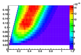
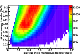
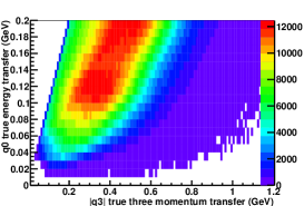
As a temporary mitigation, we have multiplied the global iteration max kRjMaxIterations ( default = 1000 ) by 1000 for this specific loop, an earlier test with 100 times default is illustrated in Fig. 9. The left plot has a high statistics event rate distribution from the IFIC Valencia modle calculation directly. The other two are 50M stats samples from GENIE which allow 100,000 (center) and 1,000 (right) rejections. The sculpting is visible in the lower left corner of each plot, and in the lower right corner of the right-most two (equal-stats) plots.

Ordinarily the solution is to impose a kinematic maximum as a function of the energy transfer, and throw for nucleons within that maximum, resulting in acceptably small iterations even at this kinematic limit. In this case, we are using a method from the nuclear model class, so we don’t see an easy way to impose a limit from within the MECTensor model.

Caution: switching to even more wacky nuclear models (local fermi gas or spectral function) might exacerbate the problem caused by terminating this loop.

Of course, we are not changing the total cross section at all, because that is set by the spline. What we are doing is enhancing the rest of the kinematic region’s double differential cross section by an amount that is less than 0.01% of the total, but getting this corner wrong by 1%. This seems acceptable.

One other artifact is visible in Fig. 9. The GENIE based plots have event rate below $q_{0}$ = 0.02 GeV, but the IFIC Valencia model calculation does not. This is coming not from physics, but from the 2D interpolation method. The model authors coded it in a way that gives a limit at the first bin of the table, which corresponds to $q_{0}$ = 0.021 GeV for carbon. The GENIE interpolator assumes the table goes to zero just outside the bounds of the table, and is willing to interpolate into this. In principle this affects both the spline and the differential cross sections by about 1%.

4.7 Removal energy when generating the hadron system

The IFIC Valencia model lepton tensor calculation considers particular choices about the CC process Q-value for protons or neutrons and the three isoscalar nuclei ¹²C, ¹⁶O, ⁴⁰Ca in Table I of the QE+RPA paper [3], or from any table of nuclei. With the incorporation of this model, we updated GENIE’s model for nuclear masses to the latest complete compilation [15]. For some common remnant nuclei like C11, this was a change of 10 MeV and has a Q-value-like effect on the energy of the outgoing products, especially the lepton for QE events.

Beyond that, the Valencia code integrates over the specifics of initial and final hadron states, so that aspect of the model is not available to us. In this case, the GENIE version of those specifics are substituted.

The initial state hadrons are not drawn from the same local fermi gas used in the Valencia model. We follow the user’s choices for GENIE’s nuclear environment. The method here almost matches how GENIE treats removal energy in the CCQE case, and is slightly different than what NuWro does. The nucleon cluster is formed from two nucleons drawn randomly from the prevailing nuclear model.

Most nuclear models in GENIE also assign a removal energy to nucleons. The default Fermi-gas model considers the removal energy a constant 25 MeV for carbon, regardless of the momentum assigned to the nucleon. Alternate models such as a spectral function draw a removal energy explicitly from a probability distribution function when choosing a nucleon. In contrast, a local Fermi-gas would correlate the removal energy with the local nuclear density.

These two quantities (one for each removed nucleon) of removal energy are subtracted from the energy transfer and added to the remnant (excited) nucleus. In the versions of GENIE up to now (2.12.6 and earlier), this energy is unavailable and is not transferred to the Geant4 system for most or all nuclei. In the case of NuWro [9], this same thing is done, but after the di-nucleon cluster is split, then an additional 8 MeV of binding energy is removed from each nucleon “to put it on shell”.

GENIE technical point. There is a second mechanism for accounting for where removal energy within GENIE ends up. It can attached to a neutron or proton using the SetRemovalEnergy method. When the event is complete, all the final particles are queried to determine if there is a stored removal energy, and they are placed in the event record as a final state particle called “NucBindE” with the removal energy (e.g. 25 MeV) appropriate for that nucleus. This method is only used for protons and neutrons, and are visible especially in quasi-elastic events.

GENIE physics point. The above two methods lead to the same result: there are one or more particles in the final state that will not usually lead to energy deposit or deexcitation, but should and may contain 25 to 100 MeV or even more energy. At this point in GENIE, it doesn’t matter whether its in the form of a HadBlob or NucBindE, it will be ignored when passed to Geant4. There are plans within GENIE to improve this. The MINERvA data on the calorimetric hadron system [5] has some sensitivity to the unsimulated portion of this energy that appears promptly in the form of additional ejected nucleons or deexcitation photons if they happen within 35 ns or 150 ns, depending on the specifics of the analysis. (MINERvA would also be sensitivite to radiative processes producing a photon and modifying the lepton kinematics).

4.8 Decay the nucleons

The implementation calls ROOT’s TGenPhaseSpace class, which was based on the GENBOD W515 n-body event generator. The ROOT class further mentions it uses the Raubold and Lynch method, and is also documented in F. James, Monte Carlo Phase Space, CERN 68-15 (1968).

Most information about the separate initial states of each nucleon is lost, only the combined three-momentum and energy, and the isospin state, is passed to the phase space decayer. This is obviously a simplification that ignores details at are buried in inner integrations of the IFIC Valencia model calculations. We have chosen to live with for this early implementation.

This class will make a two-particle system back-to-back and isotropic in the center of momentum frame, then boost it back into the “lab frame” of the particle that was passed to the class. It returns a weight, which must be queried with a random number followed by rethrow if the random number test fails. This weight presumably doesn’t matter (?) for isotropic two-body decays, but gets the distribution of three-body decays right.

Using this fancy isotropic decayer is unnecessary if all we ever cared to do was two nucleons. In principle, the code is prepped to extend this model to include some 3p3h states, and still use this phase space decayer, which does appropriately more interesting things in this case.

5 What to do about the Delta component

The calculation is NOT of an inclusive 2p2h process, it is of the QE-like (no pion) component of the 2p2h process. Even then, it excludes the QE-like 1p1h with SRC diagrams, which Nieves instead incorporates in his RPA model.

The hadron tensor explicitly includes a portion of the cross section with Delta kinematics, with a Delta produced at the diagram level which “decays” back to a nucleon during the eponymous meson exchange, or maybe the $\Delta$ is “absorbed” at the diagram level. This happens before any $\Delta$, pion, or nucleon is passed to the Final State Interaction model. In this model, such delta events still have an “experimenter’s W” invariant mass of approximately 1.232 GeV.

The total calculation of the amplitudes includes terms with and without the Delta, but not with higher order resonances. There are significant interference terms that do not change the cross section compared to ignoring the Delta amplitudes, but do significantly change where in the kinematics the cross section sits, and where the pn initial states are the highest.

About 16% of the deltas produced by the GENIE default model already lose their pion in the FSI model to some absorption/knockout process, leading to two or more nucleons in the final state. A similar number of events are predicted by this 2p2h model to have delta kinematics but with two nucleons and no pion, before FSI. A core prediction of the model is that there will be more nucleon-only events in a QE+delta kinematic sample than a prediction without this process. Other generators, such as NEUT, have an available pionless delta decay mode.

The effect of the interference is clear for the QE-like sample, but it is not so clear for the inclusive sample. Do the pionless delta decay/absorption events take the place of 1p1h (and/or 2p2h) delta events with a pion, or are they in addition to those, or somewhere in between.

Given the nature of the prediction, it makes sense to ask this model to generate all the 2p2h pionless delta component, and pass the result to FSI. Simultaneously, the user should generate 1p1h deltas and pass their products to the FSI model, some of which will lose their pion. Then the user (concerned about model-dependent systematic effects) might consider the following two extremes. One is to keep the 1p1h delta strength as it is (informed by deuterium data and other evidence), the other is to reduce the 1p1h delta strength by the amount of 2p2h pionless delta produced. An inclusive calculation would presumably yield something in between, and/or have something specific to say about the isospin states involved.

The facility to do the above can be accomplished because the model presented here includes the Delta-only hadronic tensor, and can calculate the resulting cross section on its own. With that, the presence of the Delta in the generated can be tagged statistically for each interaction with the internal computation of two more cross sections and additional random throws. On an event-by-event basis, this is saved as the Delta resonance type (xcls.Resonance() == 0) ; This allows the user the option to generate the events from the total Nieves model, but then weight the Delta-induced component to zero in favor of their other favorite pionless-Delta model, like the one that has been available in NEUT or a weighting up of the FSI version. Note, users of this version of GENIE who already (from past versions) use the resonance ID method should also query the interaction type for resonance or 2p2h, if that distinction is important for analysis.

6 What to do about other nuclei

The implementation in GENIE from 2.12.6 onward generates interactions all nuclei with A $\geq$ 9, gives a rough guess for helium-4 (needed today only by MINERvA). It does this by creating a set of hadron tensors for a few specific nuclei that span the periodic table and scaling to any nearby nuclei the user requests.

He4	$\sim$ from carbon 12	MINERvA special
other A $<$ 9	not available
9 $\leq$ A $<$ 15	carbon 12	will give N14
15 $\leq$ A $<$ 22	oxygen 16
22 $\leq$ A $<$ 33	silicon 28	will give Al27
33 $\leq$ A $<$ 50	calcium 40	will give Ar40, Ti48
50 $\leq$ A $<$ 90	Ni56 = pseudoFe	will give Fe
90 $\leq$ A $<$ 160	Ba112 = pseudoCd
160 $\leq$ A	Rf208 = pseudoPb

Table 1: Hadron tensor used for the range of nuclei in GENIE. The PseudoA means the code used an isoscalar nuclei with the density parameters of Fe, Cd, and Pb.

The IFIC Valencia model and the hadron tensors are based on isoscalar nuclei. However, the version of the model that uses hadron tensors approximately scales with A, and combinatorics can be used make a prediction for nuclei that are not isoscalar.

The strategy is to start with isoscalar nucleus with A near each of the nuclei we expect users will want. Then a good approximation is to scale the pn (and the not-pn) initial fraction to account for the different number of protons and neutrons in a nucleus of the same A. That same scaling will naturally account for a slightly different A, as long as it is not too different.

For example, to get ${}^{40}_{18}$Ar from ${}^{40}_{20}$Ca, which have the same A, we should first take the probability that we had an initial pn pair in Argon (22x18) divide by those in Calcium (20x20), and use that as the scaling factor 0.99. In fact, this prescription would cause the cross section to scale as $A^{2}$, which is not desired, so taking the square root returns a factor even closer to 1.0. Likewise, scale the initial nn pairs by Sqrt( (22x21/2) / (20x19/2) ) = 1.10 and apply those scales to the appropriate components and reform the total cross section. Something similar for initial pp pairs in the anti-neutrino case, (18x17/2)/(20x19/2) then the square root yielding 0.897. This strategy extends to one other vital nucleus, where we could approximate ⁵⁶Fe scaling from ⁵⁶Ni.

Higher on the periodic table, there are no naturally occuring isoscalar nuclei on which to base the hadron tensor. The calculation was asked to produce tensors for barium 112 and Rutherfordium 208, but was told to use the nuclear density parameters for cadmium and lead respectively. Even the example above, using iron is more likely than nickel, so the hadron tensor for isoscalar A=56 was generated with the iron density parameters, though they are not very different. Then the scaling away from isoscalar proceeds as before. That is quite a big scaling from Rf208 to Pb208, and it is difficult to evaluate the accuracy of the result, except it is certainly a better approximation than having no QE-like 2p2h component at all.

The author’s code uses nuclear density parameters to approximate these nuclei, which is not tested and may not be appropriate for helium. Neverthelsess, He4 is added for the 2017 release of GENIE 2.12.6, to satisfy the immediate need for some generated events from helium for use with data from the MINERvA experiment. The code will generate events for helium using the above prescription, and the carbon hadron tensor as input, plus the actual Q-value for helium. This will produce 1/3 the events on pn pairs, and the combinatorics will yield 1/4 the events on pp and nn pairs. It is not suitable to consider these events as predictions of the model, and any study doing so should state so. But the resulting events could be used to evaluate acceptance and resolution effects and study potential sensitivity to future models. GENIE will not produce events on D, T, He3, nor Li based on this model.

In the 2013 paper [2], it was reported that the Delta component did not scale exactly with A. That paper used two variations of the calculation, and the latter variation that separates out the hadron tensor calculation does not have that strong, non-A scaling behavior. Therefore, the GENIE implementation also scales very nearly with A.

This prescription leads to three kinds of differences between any two nuclei. The scaling of pn, pp, nn is clear from the discussion above. Another comes from the applicaiton of Q-value. The third comes from the choice of nuclear density parameters, if different nuclei are widely separated on the periodic table.

Figure 10: Comparison of the three components that come into play when comparing two nuclei. The left shows the ratio of Ca40 over C12, forcing Ca40 to have the C12 Q-value, so only the nuclear density parameters and total A are different. The middle shows the scaling away from isoscalar nuclei Ar40/Ca40, giving the numerator the same Q-value as the Ca40. The slight statistically significant differences enhance the !pn component. The right plot isolates the Q-value effect, computing Ar40/Ar40 with the denominator having the Q-value for Ca40 but no other differences.

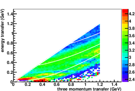
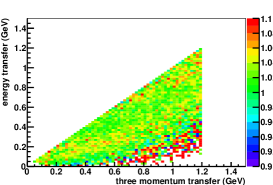
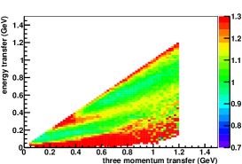
A comparison is made of the calculation using the nuclear density parameters for Ca40 and C12, but both are isoscalar and the comparison artifically sets the same Q value. This comparison is in the left plot of Fig. 10. This yields 30% changes in the regions where there was little event rate, and some 10% artifacts in the QE region that follow lines of the internal numerical integrations. There could be 5% effects beyond A scaling in the pp and nn initial state reactions.

The most extreme changes in Q-value cause noticeable changes in the cross section, shown in the far right plot of Fig. 10. Despite being very nearby, stable nuclei, neutrino reactions on Ar40 has Q = 1 MeV while Ca40 is 14 MeV. This causes the entire cross section distribution to shift down or up by that 13 MeV. With the peaked distribution, this causes 30% changes in regions where there was little event rate to begin with, and -10% changes at the peaks. This modification of the kinematic space can also cause nearly 10% changes in the integrated cross section.

The middle plot shows the effect of the pn and nn scaling to a nucleus with relatively more neutrons in the initial state. The statistics of the sample, the smallness of the effect (Ar40 and Ca40 are near to each other), and that its diluted from combining pn and nn at the same time, mean its hard to see. The trend indeed follows from the upper right plot of Fig. 1.

7 Model comparisons, tuning, uncertainties

There are many models on the market. This section has been updated to include the most prominent as of early 2017. Apples to apples comparisons between these models are rare, comparisons to the same data sets are more common.

GENIE has a W-parameterized model built by Steve Dytman [16] inspired by the Quasi-Free Scattering model implemented in FORTRAN of Lightbody and O’Connell [17] in the 1980s. This model was available in the early days of JLab, and was used in proposals to pursue 2N signatures in electron scattering data and other inclusive reaction studies. Like our need, this code included QE scattering, two-nucleon knockout in the dip region, the Delta and the next two resonances, and a DIS component. The original version used a Cauchy/Lorentz/Breit-Wigner distribution as would be normal for the $\Delta$ resonance. In the current Dytman implementation for GENIE, the MEC component is simplified a Gaussian distribution in W centered on 2.1 GeV with a width of 0.5 GeV and $Q^{2}$ peaked near zero. This corresponds to 225 MeV of kinetic energy available in the center of momentum frame once the nucleons separate, and should place these events somewhere between the QE and the Delta, in the dip region of the usual kinematic spaces. Since GENIE version 2.10.6 it takes the fraction of initial-state di-nucleon clusters to be 80% pn, for both neutrino and anti-neutrino. Some of these parameters can be configured to other values in the options file. Also since this version, the cross section no longer rolls off at 5 GeV by design. This was a way to balance the potential disagreement between the MiniBooNE and NOMAD results, but that explanation was ruled out by MINERvA data [5]. This previous energy dependent behavior was similar to the proposal of the Transverse Enhancement Model inspired by inclusive electron scattering data.

The model of Martini and Ericson [8] is the successor to earlier work of Marteau [18]. Marteau’s work itself was based on prior work by Ericson an Delorme in the 1980s. This overall effort is sometimes referred to as the “Lyon Model”, though here we’ll refer to its main proponent and call it Martini’s model. The diagrams they compute are similar to the IFIC Valencia model, but as of 2014 were missing a few diagrams that Nieves includes. Some versions of this model are non-relativistic, while other version contain progress toward a more completely relativistic calculation. Also, the overall cross section predicted by Martini’s model is about a factor of two larger than the IFIC Valencia model, though both describe electron scattering data similarly. Maybe it includes the SRC component that Nieves leaves to his RPA model. Detailed comparisons of the two models at the range of energies of interest are few and limited.

A comparison of the Martini and Nieves models and a subset of MiniBooNE data is in the ICHEP2014 conference proceedings [19], illustrating the normalization difference, and suggesting the Martini model produces events closer to the central QE kinematics (further from the center of the dip) than the IFIC model does. Some of the technical differences between these two approaches are highlighted in the introduction to [20].

Additional progress has been made in collaboration with Martini and Jachowicz and their students in Gent, especially Van Cuyck [21, 22] to accompany their work on the quasielastic process. Broad comparisons to other models are not yet available. The precursor to Martini’s Model, by Marteau [18], is implemented in the NuWro generator, and numerous predictions and comparisons to what is presented in this note might be readily obtained if we ask the NuWro experts. There are a number of NuWro talks on this topic, including comparisons with the IFIC Valencia model.

A campaign has been launched by proponents of the superscaling (SuSA) approach, including work by Megias, plus also Nieves and Vicente’s former student, Ruiz Simo. This effort builds off the work by De Pace, et al. [23] which was a microscopic calculation of 2p2h effects in electron scattering. This previous effort augmented the authors work on the SuperScaling (SuSA) description of the QE and $\Delta$ processes, so they could describe inclusive electron scattering including a component in the “dip region” that probably does not obey superscaling. Ruiz Simo is investigating the full computation of the 2p2h process, adding the axial terms, and doing so without the simplifications that yield a hadronic tensor with only four or two dimensional integrations and 8 cpucore.days worth of computation. Progress thus far has been described in [20, 10, 24, 25, 26, 27, 28, 29], which cover a mix of physics and computational challenges, with careful but limited comparisons to simpler or asymptotic approaches.

The transverse enhance model [30] extracts an enhancement from (e,e’) inclusive electron scattering, and notes that the enhancement appears only in the transverse channel. The model is then applied by scaling the magnetic form factors in the QE case. This serves to produce a prediction for the total cross section $\sigma(E)$. But because it is designed around a reweight of QE interactions, it can not capture the complexity that the more detailed models do. Certainly, such an implementation would poorly predict the energy transfer and nucleon kinematics.

tuning options and uncertainties.

This is an area for further exploration, especially as additional modeling efforts described above mature. As of this writing, we have not been so creative about what is needed. Early readers of this document might suggest a few things to look at.

By construction, the Nieves model takes only one parameter from neutrino data, the Axial vector mass (assuming a dipole), which historically they have set to $M_{A}=1.05$ GeV. Likewise there is a treatment of the Delta axial form factor. In that sense, it is the only thing available to be tuned. Changing $M_{A}$ probably has normalization effect more than anything else, with some mild $Q^{2}$ effect.

Of course, experimentalists are more creative than that. All current models listed above simplify something to allow calculations to proceed with reasonable time, and neutrino-nucleus data sets still beg for creative interpretation of models. So variations between models, expressed as a normalization or magnitude might be an okay way to start. As the community enhances our ability to compare models to neutrino-nucleus data, that may suggest some additional targeted constraints.

Its conceivable to change the assumptions about where the model draws nucleons and what it does with them. For example, code up a blatantly asymmetric sharing of energy and momentum transfer, or make the sharing artificially more symmetric than the Lorentz boost. As it is, the model seems to produce as moderate a result as could be expected.

Finally, one could shave off near the momentum-transfer limit from 1.0 to 1.2 GeV, or enhance it. This might be especially important if someone’s analysis is sensitive to the region where the model is truncated. The tail of the distribution of a background process for some DIS study, for example.

References

- [1] J. Nieves, I. Ruiz Simo, M. Vicente Vacas, Inclusive Charged–Current Neutrino–Nucleus Reactions, Phys. Rev. C83 (2011) 045501. arXiv:1102.2777, doi:10.1103/PhysRevC.83.045501.
- [2] R. Gran, J. Nieves, F. Sanchez, M. Vicente Vacas, Neutrino-nucleus quasi-elastic and 2p2h interactions up to 10 GeV, Phys.Rev. D88 (2013) 113007. arXiv:1307.8105, doi:10.1103/PhysRevD.88.113007.
- [3] J. Nieves, J. E. Amaro, M. Valverde, Inclusive quasi-elastic neutrino reactions, Phys. Rev. C70 (2004) 055503. arXiv:nucl-th/0408005, doi:10.1103/PhysRevC.70.055503,10.1103/PhysRevC.72.019902.
- [4] J. Nieves, I. Ruiz Simo, M. Vicente Vacas, The nucleon axial mass and the MiniBooNE Quasielastic Neutrino-Nucleus Scattering problem, Phys.Lett. B707 (2012) 72–75. arXiv:1106.5374, doi:10.1016/j.physletb.2011.11.061.
- [5] P. A. Rodrigues, et al., Identification of nuclear effects in neutrino-carbon interactions at low three-momentum transfer, Phys. Rev. Lett. 116 (2016) 071802. arXiv:1511.05944, doi:10.1103/PhysRevLett.116.071802.
- [6] A. S. Meyer, M. Betancourt, R. Gran, R. J. Hill, Deuterium target data for precision neutrino-nucleus cross sections, Phys. Rev. D93 (11) (2016) 113015. arXiv:1603.03048, doi:10.1103/PhysRevD.93.113015.
- [7] R. Gran, Model uncertainties for Valencia RPA effect for MINERvA, FERMILAB-FN-1030-ND and MINERvA Note TN080 (2017) .arXiv:1705.02932.
- [8] M. Martini, M. Ericson, G. Chanfray, J. Marteau, A Unified approach for nucleon knock-out, coherent and incoherent pion production in neutrino interactions with nuclei, Phys. Rev. C80 (2009) 065501. arXiv:0910.2622, doi:10.1103/PhysRevC.80.065501.
- [9] J. T. Sobczyk, Multinucleon ejection model for Meson Exchange Current neutrino interactions, Phys.Rev. C86 (2012) 015504. arXiv:1201.3673, doi:10.1103/PhysRevC.86.015504.
- [10] I. R. Simo, C. Albertus, J. E. Amaro, M. B. Barbaro, J. A. Caballero, T. W. Donnelly, Angular distribution in two-particle emission induced by neutrinos and electrons, Phys. Rev. D90 (5) (2014) 053010. arXiv:1407.7122, doi:10.1103/PhysRevD.90.053010.
- [11] R. Gran, et al., Measurement of the quasi-elastic axial vector mass in neutrino-oxygen interactions, Phys.Rev. D74 (2006) 052002. arXiv:hep-ex/0603034, doi:10.1103/PhysRevD.74.052002.
- [12] J. Nieves, F. Sanchez, I. Ruiz Simo, M. Vicente Vacas, Neutrino Energy Reconstruction and the Shape of the CCQE-like Total Cross Section, Phys. Rev. D85 (2012) 113008. arXiv:1204.5404, doi:10.1103/PhysRevD.85.113008.
- [13] M. Martini, M. Ericson, G. Chanfray, Energy reconstruction effects in neutrino oscillation experiments and implications for the analysis, Phys.Rev. D87 (2013) 013009. arXiv:1211.1523, doi:10.1103/PhysRevD.87.013009.
- [14] U. Mosel, O. Lalakulich, K. Gallmeister, Energy reconstruction in the Long-Baseline Neutrino Experiment, Phys.Rev.Lett. 112 (2014) 151802. arXiv:1311.7288, doi:10.1103/PhysRevLett.112.151802.
-
[15]
M. Wang, G. Audi, A. Wapstra, F. Kondev, M. MacCormick, X. Xu, B. Pfeiffer,
The ame2012 atomic mass
evaluation, Chinese Physics C 36 (12) (2012) 1603.
URL http://stacks.iop.org/1674-1137/36/i=12/a=003 - [16] T. Katori, Meson Exchange Current (MEC) Models in Neutrino Interaction Generators, proceedings of NuInt12 Rio de Janeiro, Brazil, AIP Conf.Proc. 1663 (2015) 030001. arXiv:1304.6014, doi:10.1063/1.4919465.
- [17] J. W. Lightbody, J. S. O’Connell, Modeling single arm electron scattering and nucleon production from nuclei by GeV electrons, Computers in Physics 2 (1988) 57.
- [18] J. Marteau, Effects of the nuclear correlations on the neutrino oxygen interactions, Eur. Phys. J. A5 (1999) 183–190. arXiv:hep-ph/9902210, doi:10.1007/s100500050274.
[19]
J. Nieves, R. Gran, I. R. Simo, F. Sanchez, M. J. V. Vacas,
Neutrino-nucleus
CCQE-like scattering, in: proceedings of the International Conference on
High Energy Physics 2014 (ICHEP 2014) Valencia, Spain, July 2-9, 2014, 2014.
arXiv:1411.7821.
URL http://inspirehep.net/record/1331445/files/arXiv:1411.7821.pdf - [20] I. Ruiz Simo, C. Albertus, J. E. Amaro, M. B. Barbaro, J. A. Caballero, T. W. Donnelly, Relativistic effects in two-particle emission for electron and neutrino reactions, Phys. Rev. D90 (3) (2014) 033012. arXiv:1405.4280, doi:10.1103/PhysRevD.90.033012.
- [21] T. Van Cuyck, N. Jachowicz, R. González-Jiménez, M. Martini, V. Pandey, J. Ryckebusch, N. Van Dessel, Influence of short-range correlations in neutrino-nucleus scattering, Phys. Rev. C94 (2) (2016) 024611. arXiv:1606.00273, doi:10.1103/PhysRevC.94.024611.
- [22] T. Van Cuyck, N. Jachowicz, R. González-Jiménez, J. Ryckebusch, N. Van Dessel, Seagull and pion-in-flight currents in neutrino-induced and knockoutarXiv:1702.06402.
- [23] A. De Pace, M. Nardi, W. M. Alberico, T. W. Donnelly, A. Molinari, The 2p - 2h electromagnetic response in the quasielastic peak and beyond, Nucl. Phys. A726 (2003) 303–326. arXiv:nucl-th/0304084, doi:10.1016/S0375-9474(03)01625-7.
- [24] G. D. Megias, et al., Meson-exchange currents and quasielastic predictions for charged-current neutrino- scattering in the superscaling approach, Phys. Rev. D91 (7) (2015) 073004. arXiv:1412.1822, doi:10.1103/PhysRevD.91.073004.
- [25] I. Ruiz Simo, J. E. Amaro, M. B. Barbaro, A. De Pace, J. A. Caballero, T. W. Donnelly, Relativistic model of 2p-2h meson exchange currents in (anti)neutrino scattering, J. Phys. G44 (6) (2017) 065105. arXiv:1604.08423, doi:10.1088/1361-6471/aa6a06.
- [26] I. Ruiz Simo, J. E. Amaro, M. B. Barbaro, A. De Pace, J. A. Caballero, G. D. Megias, T. W. Donnelly, Emission of neutron–proton and proton–proton pairs in neutrino scattering, Phys. Lett. B762 (2016) 124–130. arXiv:1607.08451, doi:10.1016/j.physletb.2016.09.021.
- [27] G. Megias, J. Amaro, M. Barbaro, J. Caballero, T. Donnelly, I. Ruiz Simo, Charged-current neutrino-nucleus reactions within the superscaling meson-exchange current approach, Phys. Rev. D94 (9) (2016) 093004. arXiv:1607.08565, doi:10.1103/PhysRevD.94.093004.
- [28] I. Ruiz Simo, J. E. Amaro, M. B. Barbaro, J. A. Caballero, G. D. Megias, T. W. Donnelly, The frozen nucleon approximation in two-particle two-hole response functionsarXiv:1703.01186.
- [29] J. E. Amaro, M. B. Barbaro, J. A. Caballero, A. De Pace, T. W. Donnelly, G. D. Megias, I. Ruiz Simo, Density dependence of 2p-2h meson-exchange currentsarXiv:1704.01539.
- [30] A. Bodek, H. S. Budd, M. E. Christy, Neutrino Quasielastic Scattering on Nuclear Targets: Parametrizing Transverse Enhancement (Meson Exchange Currents), Eur. Phys. J. C71 (2011) 1726. arXiv:1106.0340, doi:10.1140/epjc/s10052-011-1726-y.