Atomistic Description for Temperature–Driven Phase Transitions in BaTiO₃

Abstract

Barium titanate (BaTiO₃) is a prototypical ferroelectric perovskite that undergoes the rhombohedral–orthorhombic–tetragonal–cubic phase transitions as the temperature increases. In this work, we develop a classical interatomic potential for BaTiO₃ within the framework of the bond–valence theory. The force field is parameterized from first–principles results, enabling accurate large–scale molecular dynamics (MD) simulations at finite temperatures. Our model potential for BaTiO₃ reproduces the temperature–driven phase transitions in isobaric–isothermal ensemble ($NPT$) MD simulations. This potential allows the analysis of BaTiO₃ structures with atomic resolution. By analyzing the local displacements of Ti atoms, we demonstrate that the phase transitions of BaTiO₃ exhibit a mix of order–disorder and displacive characters. Besides, from detailed observation of structural dynamics during phase transition, we discover that the global phase transition is associated with changes in the equilibrium value and fluctuations of each polarization component, including the ones already averaging to zero, Contrary to the conventional understanding that temperature increase generally causes bond–softening transition, the $x$ polarization component exhibits a bond–hardening character during the orthorhombic to tetragonal transition. These results provide further insights about the temperature–driven phase transitions in BaTiO₃.

I Introduction

BaTiO₃ is a ferroelectric perovskite with promising applications in electronic devices, such as non–volatile memory, high–$\kappa$ dielectrics, and piezoelectric sensors Yun et al. (2002); Chen et al. (2007); Buessem et al. (1966); Karaki et al. (2007). Therefore, it is of great significance to investigate and understand the structural and electronic properties of BaTiO₃ for designed material optimization and device engineering. First–principles density functional theory (DFT) has served as a powerful method to understand the electronic structures of ferroelectric materials Cohen (1992); Gonze and Lee (1997); Saha et al. (2000); Kolpak et al. (2008); Martirez et al. (2012); Morales et al. (2014). Due to the expensive computational cost, the application of DFT methods is currently limited to system of fairly small size at zero Kelvin. Many important dynamical properties, such as domain wall motions and temperature–driven phase transitions, are beyond the capability of conventional first–principles methods. An effective Hamiltonian method was developed to study finite–temperature properties of BaTiO₃ Zhong et al. (1994, 1995); Nishimatsu et al. (2008); Fu and Bellaiche (2003). To apply this method, the subset of dynamical modes that determine a specific property should be known a priori. Molecular dynamics (MD) simulations with an atomistic potential accounting for all the modes offer distinct advantages, especially in providing detailed information about atomic positions, velocities and modifications of chemical bonds due to a chemical reaction or thermal excitation. The shell model for BaTiO₃ has been developed Tinte et al. (1999); Tinte and Stachiotti (2001); Tinte et al. (2000); Zhang et al. (2010, 2009). However, due to the low mass assigned to the shell, a small time step in MD simulations is required to achieve accurate results, which limits the time and length scales of the simulations.

Recently, we developed a bond–valence (BV) model potential for oxides based on the bond valence theory Grinberg et al. (2002); Shin et al. (2008, 2005); Liu et al. (2013a, b). The force fields for many technologically important ferroelectric materials, PbTiO₃, PbZrO₃ and BiFeO₃ Liu et al. (2013a, b); Shin et al. (2005); Grinberg et al. (2002); Chen et al. (2015), have been parameterized based on results from DFT calculations. A typical force field requires no more than 15 parameters and can be efficiently implemented, which enables simulations of systems with thousands of atoms under periodic boundary conditions Liu et al. (2013c); Xu et al. (2015). The development of an accurate classical potential for BaTiO₃ has proven to be difficult, mainly due to the small energy differences among the four phases (rhombohedral, orthorhombic, tetragonal, and cubic) Kwei et al. (1993); Diéguez et al. (2004); Von Hippel (1950). In this paper, we apply the bond–valence model to BaTiO₃ and parameterize the all–atom interatomic potential to first–principles data. Our model potential for BaTiO₃ is able to reproduce the rhombohedral–orthorhombic–tetragonal–cubic (R-O-T-C) phase transition sequence in isobaric–isothermal ensemble ($NPT$) MD simulations. The phase transition temperatures agree reasonably well with previous theoretical results Tinte et al. (1999). We further examine the temperature dependence of the local displacements of Ti atoms and discover several features of the phase transitions of BaTiO₃: the phase transitions of BaTiO₃ involve both order–disorder and displacive characters; at the moment that the phase transition of the crystal occurs, all the polarization components undergo phase transitions, even for the nonpolar ones; and temperature increase can also cause bond–hardening for a certain component.

II Methods

The bond–valence model potential is developed based on the conservation principles of bond valence and bond–valence vector. The bond valence, $V_{ij}$, reflects the bonding strength and can be calculated based on the bond length, $r_{ij}$, with Brown (2009); Grinberg et al. (2002); Brown and Shannon (1973); Brown and Wu (1976); Liu et al. (2013a, b); Shin et al. (2008, 2005)

$$V_{ij}=\left(\frac{r_{0,ij}}{r_{ij}}\right)^{C_{ij}}$$ (1)

where $i$ and $j$ are the labels for atoms; $r_{0,ij}$ and $C_{ij}$ are Brown’s empirical parameters. The bond–valence vector is defined as a vector lying along the bond, ${\bf{V}}_{ij}=V_{ij}\hat{{\bf{R}}}_{ij}$, where $\hat{{\bf{R}}}_{ij}$ is the unit vector pointing from atom $i$ to atom $j$. The total energy ($E$) consists of the Coulombic energy ($E_{c}$), the short–range repulsive energy ($E_{r}$), the bond–valence energy ($E_{\rm BV}$), the bond–valence vector energy ($E_{\rm BVV}$), and the angle potential ($E_{a}$) Liu et al. (2013a, b); Shin et al. (2008, 2005):

$$E=E_{c}+E_{r}+E_{\rm BV}+E_{\rm BVV}+E_{a}$$ (2)

$$E_{c}=\sum_{i<j}\frac{q_{i}q_{j}}{r_{ij}},$$ (3)

$$E_{r}=\sum_{i<j}\left(\frac{B_{ij}}{r_{ij}}\right)^{12},$$ (4)

$$E_{\rm BV}=\sum_{i}S_{i}\left(V_{i}-V_{0,i}\right)^{2}$$ (5)

$$E_{\rm BVV}=\sum_{i}D_{i}\left({\bf{W}}_{i}^{2}-{\bf{W}}_{0,i}^{2}\right)^{2}$$ (6)

$$E_{a}=k\sum_{i}^{N_{\rm oxygen}}\left(\theta_{i}-180^{\circ}\right)^{2}$$ (7)

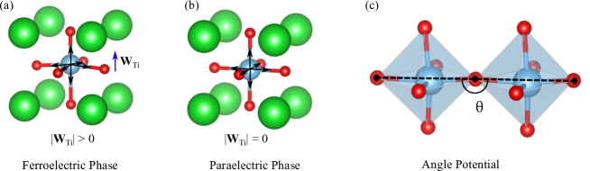
Figure 1: Bond valence vector sum and angle potential. (a) Tetragonal BaTiO₃ with a non-zero BVVS; (b) Cubic BaTiO₃ with zero BVVS; (c) Schematic of the angle potential. Ba, Ti, and O atoms are represented by green, blue and red spheres respectively.

where ${V}_{i}=\sum_{j\not=i}V_{ij}$ is the bond–valence sum (BVS), ${\bf{W}}_{i}=\sum_{j\not=i}{\bf{V}}_{ij}$ is the bond–valence vector sum (BVVS, shown in FIG. 1 (a), (b)), $q_{i}$ is the ionic charge, $B_{ij}$ is the short–range repulsion parameter, $S_{i}$ and $D_{i}$ are scaling parameters with the unit of energy, $k$ is the spring constant and $\theta$ is the O–O–O angle along the common axis of two adjacent oxygen octahedra (FIG. 1 (c)). The bond-valence energy $E_{\rm BV}$ captures the energy penalty for both overbonded and underbonded atoms. The bond-valence vector energy $E_{\rm BVV}$ is a measure of the breaking of local symmetry, which is important for correctly describing the ferroelectricity. $V_{0,i}$ and ${\bf{W}}_{0,i}$ are preferred or target values of BVS and BVVS for atom $i$ in the ground–state structure, which can be calculated from DFT directly. It is noted that the $E_{\rm BV}$ and $E_{\rm BVV}$ can be related to the moments of the local density of states in the framework of a tight binding model, providing a quantum mechanical justification for these two energy terms Liu et al. (2013a, b); Finnis and Sinclair (1984); Brown (2009); Harvey et al. (2006). The angle potential is used to account for the energy cost associated with the rotations of oxygen octahedra.

We followed the optimization protocol developed in previous studies Liu et al. (2013a, b). The optimal values of force-field parameters $q_{i}$, $S_{i}$, $D_{i}$ and $B_{ij}$, are acquired by minimizing the difference between the DFT energies/forces and the model–potential energies/forces for a database of BaTiO₃ structures. All DFT calculations are carried out with the plane–wave DFT package Quantum–espresso Giannozzi et al. (2009) using the Perdew–Burke–Ernzerhof functional modified for solids (PBEsol) Perdew et al. (2008) and optimized norm–conserving pseudopotentials generated by the Opium package Opi . A plane–wave cutoff energy of 50 Ry and 4$\times$4$\times 4$ Monkhorst–Pack $k$–point mesh Monkhorst and Pack (1976) are used for energy and force calcualtions. The database consists of 40–atom 2$\times$2$\times$2 supercells with different lattice constants and local ion displacements. The final average difference between DFT energy and model–potential energy is 1.35 meV/atom.

III Performance of the classical potential

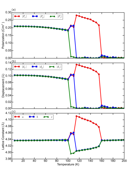
Figure 2: Temperature dependence of the polarization, Ti displacement, and lattice constants in BaTiO₃. Phase transitions between rhombohedral, orthorhombic, tetragonal, and cubic occur at 105 K, 115 K and 160 K.

The optimized parameters are listed in TABLE 1. The performance of the obtained force field is examined by investigating the temperature dependence of lattice constants ($a$, $b$ and $c$), component–resolved local displacements of Ti atoms ($d_{x}$, $d_{y}$, and $d_{z}$), and the three components of the total polarization ($P_{x}$, $P_{y}$, and $P_{z}$). We carry out $NPT$ MD simulations using a 10$\times$10$\times$10 supercell (5000 atoms) with the temperature controlled via the Nosé–Hoover thermostat and the pressure maintained at 1 atm via the Parrinello–Rahman barostat Parrinello and Rahman (1980). As shown in FIG. 2, the simulations clearly reveal four distinct phases under different temperature ranges and three first–order phase transitions. Below 100 K, the displacements of Ti atoms and the overall polarization of the supercell are along [111] direction ($P_{x}=P_{y}=P_{z}$), characteristic of the rhombohedral phase. At 100 K, the $z$ component of the total polarization, $P_{z}$, becomes approximately 0, indicating a phase transition from rhombohedral to orthorhombic ($P_{x}=P_{y}>0$, $P_{z}=0$). As the temperature increases further to 110 K, the total polarization aligns preferentially along $x$ direction ($P_{x}>0$, $P_{y}=P_{z}=0$) and the lattice constants have $b=c<a$. The supercell stays tetragonal until 160 K at which point the ferroelectric–paraelectric phase transition occurs. The phase transition temperatures match well with those predicted by the shell model Tinte et al. (1999) (TABLE 2). The underestimation of Curie temperature $T_{C}$ in MD simulations has been observed previously and is likely due to the systematic error of density functional used for force field optimization Liu et al. (2013a); Sepliarsky et al. (2005). We extract the averaged lattice constants at finite temperatures from MD simulations and find that they are in good agreement (error less than 1$\%$) with the PBEsol values (TABLE 3).

Domain walls are interfaces separating domains with different polarities. They are important topological defects and can be moved by applying external stimulus Liu et al. (2013c); Xu et al. (2015). The domain wall energy for a 180^∘ wall obtained from our MD simulations is 6.63 mJ/m², which is comparable to PBEsol value, 7.84 mJ/m². This indicates that our atomistic potential can be used for studying the dynamics of ferroelectric domain walls in BaTiO₃. All these results demonstrate the robustness of this developed classical potential.

IV Atomistic features of different phases

To provide an atomistic description of the different phases of BaTiO₃, we analyze the distribution of local displacements of Ti atoms in each phase. Ti displacement is defined as the distance between the Ti atom and the center of the oxygen octahedral cage of a unit cell, which scales with the magnitude of polarization.

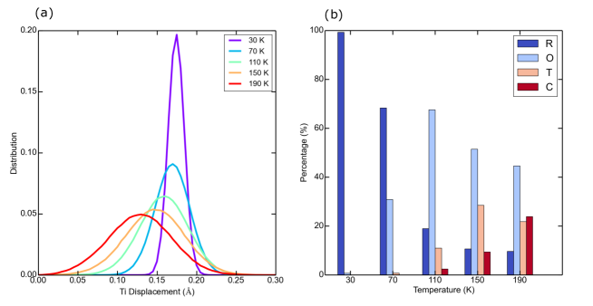
Figure 3: (a) The distribution of total Ti displacement magnitude at different temperatures. (b) Compositions of different phases. Supercells at 30 K (rhombohedral), 70 K (rhombohedral), 110 K (orthorhombic), 150 K (tetragonal) and 190 K (cubic) are studied. Heights of the dark blue, light blue, orange, and red rectangles represent the percentages of rhombohedral, orthorhombic, tetragonal and cubic unit cells respectively. The phases of unit cells are categorized by their Ti displacements $d$: for $d<0.1$ Å, the unit cell is considered as a nonpolar one; for a polar unit cell, if one component is larger than $d/\sqrt{6}$, this component is considered as a ferroelectric one. The ferroelectric phase (tetragonal, orthorhombic and rhombohedral) is determined by the number of ferroelectric components.

In FIG. 3 (a), we plot the distributions of Ti displacements ($d=\sqrt{d_{x}^{2}+d_{y}^{2}+d_{z}^{2}}$). It can be seen that in all four phases, the distribution is approximately a Gaussian curve whose peak shifts toward lower values as the temperature increases. This suggests that the temperature–driven phase transition has a displacive character. It is noted that the distribution of magnitudes is peaked at non–zero value even in the paraelectric cubic phase, suggesting that most Ti atoms are still locally displaced at high temperature, and that the overall net zero polarization is the result of an isotropic distribution of local dipoles along different directions. This confirms the order–disorder character for BaTiO₃ at high temperature.

We can categorize the phase of each unit cell based on the local displacement of Ti atom. The categorization criteria are
(1) If $d<0.1$ Å, the unit cell is considered to be paraelectric cubic;
(2) For a ferroelectric unit cell, the $k$–th component is considered to be ferroelectric if $d_{k}>d/\sqrt{6}$. The rhombohedral, orthorhombic, and tetragonal unit cells have three, two, and one ferroelectric component(s), respectively.
The results are shown in FIG. 3 (b). At 30 K, the supercell is made only from rhombohedral unit cells, showing that the rhombohedral phase is the ground–state structure. As the temperature increases, the supercell becomes a mixture of the four phases. It should be noted that the cubic unit cell with nearly–zero local Ti displacement seldom appears, because a cubic unit cell is energetically less favorable. The relative energies of the four phases of BaTiO₃ from PBEsol DFT calculations are listed in TABLE 4. It can be seen that the energy differences between the tetragonal, orthorhombic and rhombohedral unit cells are small (within several meV per unit cell) Cohen and Krakauer (1990); Cohen (1992). Due to the thermal fluctuations, the populations of higher–energy ferroelectric phases (tetragonal and orthorhombic) increase as temperature increases. Above the ferroelectric–paraelectric transition temperature, locally ferroelectric unit cells are still favored over paraelectric due to the relatively high energy of cubic, the high–symmetry structure.

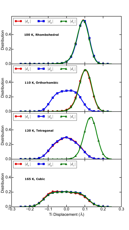
Figure 4: The distributions of Ti displacement at different temperatures.

In FIG. 4, the distributions of Ti displacements along the three axes are plotted. At 100 K, BaTiO₃ is at the rhombohedral phase and the distributions of Ti displacements are Gaussian–like. As the temperature increases, the phase changes to orthorhombic. The average of the $x$ polarization component shifts to zero, indicating a displacive phase transition. Besides, the standard deviation increases and the center of the distribution curve becomes flatter. For the cubic phase, the center of the Ti displacement distribution curve is also flat. As shown in FIG. 5, the center–flat curve is a summation of a Gaussian curve centering at zero, and a double–peak curve. The latter is characteristic of order–disorder transition Liu et al. (2013c). These results further demonstrate that phase transitions of BaTiO₃ have a mix of order–disorder and displacive characters Gaudon (2015); Ehses et al. (1981); Jun et al. (1988); Comes et al. (1968); Itoh et al. (1985); Stern (2004); Kwei et al. (1993).

V Features of the phase transitions

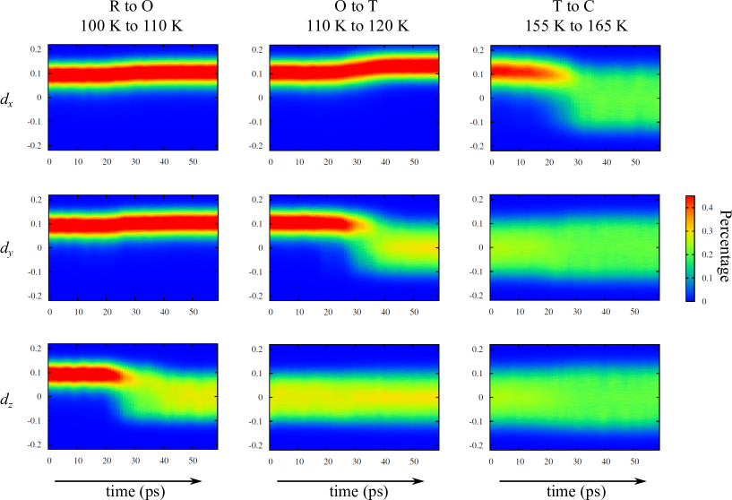
Figure 6: Temperature dependence of Ti displacement distributions in three Cartesian directions. The horizontal axis shows the time. In these simulations, the temperature increases with time approximately linearly. The vertical axis represents the fraction of the Ti displacements and the color scale represents the percentages of Ti displacement with a certain value. Note that in the bottom center plot, the color showing the distribution becomes redder after the orthorhombic to tetragonal transition, indicating a narrower distribution around $d_{z}=0$ and a bond hardening in this direction.

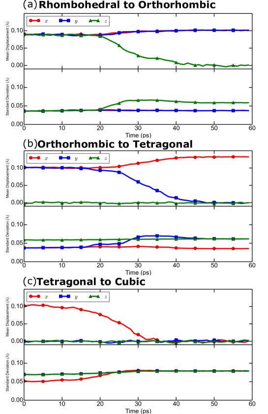
Figure 7: The change of the average and standard deviation of the Ti displacement distribution. In the standard deviation plot of (b), the green and black lines increase with temperature and are parallel until the transition.

To investigate the structural dynamics during phase transitions in more detail, we conducted MD simulations with varying temperatures. In three different sets of simulations, the temperatures were increased from 100 K to 110 K (R to O), 110 K to 120 K (O to T) and 155 K to 165 K (T to C) respectively. The temperature was controlled by the Nosé–Hoover thermostat with a thermal inertia parameter $M_{s}$=10 and the 10 K temperature change was accomplished in 60 ps. We analyze the temperature dependence of Ti displacement distributions along three axes. The dynamics of Ti displacement distributions during the phase transitions are plotted in FIG. 6. The time evolution of the average and standard deviation of the Ti displacement distributions are shown in FIG. 7.

Phase transition occurs when one component undergoes polar–nonpolar transition. The first column (from 100 K to 110 K) shows the changes of Ti displacement distributions during the rhombohedral to orthorhombic phase transition. In the $x$ and $y$ direction, the averages of the distribution shift up, which is a characteristic of displacive transition. Meanwhile, in the $z$ direction, the average becomes zero and the variance becomes significantly larger, indicating that the transition is a mix of displacive and bond–softening characters Gaffney and Chapman (2007). For the orthorhombic to tetragonal phase transition (second column), the transition of the $y$ component, which is a polar–nonpolar transition, includes both displacive and bond–softening features. For the $x$ component, the transition involves both an increase of the average and a decrease of the standard deviation. For the $z$ direction, even though the Ti displacement distribution is centered at zero above and below the transition, the Ti displacements are located closer to zero, indicating an increase in bond hardness. From 155 K to 165 K, there is also a bond–hardness–changing transition for the components ($x$ and $y$) with zero averages. We collectively refer to ‘bond–softening’ and ‘bond–hardening’ as ‘bond–hardness–changing’.

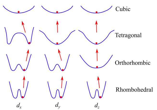
Figure 8: Schematic representations of bond–softening, bond–hardening and displacive excitations. Two points worth mentioning: (1) For the $x$ component (first column), the minima of the energy profile for the tetragonal phase are further from the center and have a higher curvature, compared with those for orthorhombic phase, because the Ti displacement distribution has a larger average and smaller variance; (2) For the $z$ component (third column), compared with the energy profile for orthorhombic phase, the one for the tetragonal phase has a higher curvature at the center (Ti displacement more closely distributed around 0, as seen from FIG. 6) and smaller curvature for larger $z$–direction displacements (larger standard deviation, seen from FIG. 7 (b)).

Based on the features of the Ti displacement distributions at different phases, the schematic representation of the thermal excitation between different energy surfaces is presented in FIG. 8. From our results, the characteristics of BaTiO₃ phase transition can be summarized as: (1) For BaTiO₃, the mechanisms of phase transitions include both bond–hardness–changing and displacive transition. The sudden shifts of the average and standard deviation correspond to displacive with some order–disorder contribution and bond–hardness–changing transitions respectively; (2) Unlike the conventional understanding that thermal excitation usually causes bond–softening, increasing temperature can also cause bond hardening. The $x$ component of polarization during the orthorhombic to tetragonal transition is an example of this case. (3) When the phase transition occurs, each component of polarization undergoes a change, even for the component(s) which is(are) non–polar before and after the transition. The transition(s) that each component undergoes are listed in TABLE 5.

VI Conclusion

In this work, we develop a classical atomistic potential for BaTiO₃ based on the bond valence model. Molecular dynamics simulation with this optimized potential can not only reproduce the temperature–driven phase transitions, but can also be a powerful tool in studying the phase transition process with high temporal and spatial resolutions. The detailed analysis of the local displacements of Ti atoms reveals that in each phase (including the paraelectric phase), the majority of Ti atoms are locally displaced, and the phase transitions in BaTiO₃ exhibit a mixture of order–disorder and displacive character. The distribution of Ti displacement is a Gaussian curve or a curve involving a Gaussian and a double peak one. Both the average and standard deviation are features of each specific phase, and they can be the order parameters for describing the Gibbs free energy. By analyzing the dynamics of Ti displacement distributions during phase transition, we discover several rules of BaTiO₃ phase transitions: the global phase transition is associated with significant changes in each component, even for the components which are nonpolar, and the orthorhombic to tetragonal transition exhibits a bond–hardening character in the $z$ component, which is opposite to the conventional understanding that temperature increase generally causes bond–softening transition.

							$B_{\beta\beta^{\prime}}\ \left({\rm{\AA}}\right)$
	$r_{0,{\beta}\rm{O}}$	$C_{0,\beta\rm{O}}$	$q_{\beta}$(e)	$S_{\beta}$(eV)	$D_{\beta}$	Ba	Ti	O	$V_{0,\beta}$	${\bf{W}}_{0,\beta}$
Ba	2.290	8.94	1.34730	0.59739	0.08429	2.44805	2.32592	1.98792	2.0	0.11561
Ti	1.798	5.20	1.28905	0.16533	0.82484		2.73825	1.37741	4.0	0.39437
O			-0.87878	0.93063	0.28006			1.99269	2.0	0.31651

Table 1: Optimized force field for BaTiO₃. The angle constant $k=6.1$ meV/(deg)².

	R–O	O–T	T–C
BV model	100 K	110 K	160 K
shell model	80 K	120 K	170 K

Table 2: Comparison of the phase transition temperatures given by the BV model and the shell model Tinte et al. (1999).

Lattice constant	MD (Å)	DFT (Å)	error
Rhombohedral
$a=b=c$	4.036	4.024	0.30$\%$
Orthorhombic
$a$	3.997	3.977	0.50$\%$
$b=c$	4.059	4.046	0.32$\%$
Tetragonal
$a=b$	4.005	3.985	0.50$\%$
$c$	4.109	4.089	0.49$\%$
Cubic
$a=b=c$	4.037	4.002	0.87$\%$

Table 3: Comparison of lattice constants of BaTiO₃ given by MD simulations with BV model potential and PBEsol DFT calculations. For MD simulation, lattice constants of rhombohedral, orthorhombic, tetragonal and cubic phases are obtained at 5 K, 105 K, 120 K and 165 K respectively. Since DFT neglects thermal expansion, the results given by MD simulations, which are larger but less than 1%, demonstrate that this set of potential can predicts the lattice constants of BaTiO₃ quite well.

	Rhombohedral	Orthorhombic	Tetragonal	Cubic
Energy (meV/unit cell)	-39.31	-37.23	-29.47	0

Table 4: Relative energies (potential energies) of different phases from DFT calculations. The cubic unit cell is chosen as the reference structure.

	R to O			O to T			T to C
Component	$d_{x}$	$d_{y}$	$d_{z}$	$d_{x}$	$d_{y}$	$d_{z}$	$d_{x}$	$d_{y}$	$d_{z}$
Hardness–changing	N	N	Y	Y	Y	Y	Y	Y	Y
Displacive	Y	Y	Y	Y	Y	N	Y	N	N

Table 5: Phase–transition characters of each component. ‘Hardness–changing’ includes bond softening and bond hardening, which are characterized by the change of the standard deviation of the Ti displacement distribution.

Figure 5: Schematic figure of the distributions of Ti displacement for displacive transition, order–disorder transition and a mix of them.

References

- Yun et al. (2002) W. S. Yun, J. J. Urban, Q. Gu, and H. Park, Nano Lett. 2, 447 (2002).
- Chen et al. (2007) K.-H. Chen, Y.-C. Chen, Z.-S. Chen, C.-F. Yang, and T.-C. Chang, Appl. Phys. A Mater. Sci. 89, 533 (2007).
- Buessem et al. (1966) W. Buessem, L. Cross, and A. Goswami, J. Am. Ceram. Soc. 49, 33 (1966).
- Karaki et al. (2007) T. Karaki, K. Yan, and M. Adachi, Jpn. J. of Appl. Phys. 46, 7035 (2007).
- Cohen (1992) R. E. Cohen, Ferroelectrics 136, 65 (1992).
- Gonze and Lee (1997) X. Gonze and C. Lee, Phys. Rev. B 55, 10355 (1997).
- Saha et al. (2000) S. Saha, T. P. Sinha, and A. Mookerjee, Phys. Rev. B 62, 8828 (2000).
- Kolpak et al. (2008) A. M. Kolpak, D. Li, R. Shao, A. M. Rappe, and D. A. Bonnell, Phys. Rev. Lett. 101, 036102 (2008).
- Martirez et al. (2012) J. M. P. Martirez, E. H. Morales, W. A. Al-Saidi, D. A. Bonnell, and A. M. Rappe, Phys. Rev. Lett. 109, 256802 1 (2012).
- Morales et al. (2014) E. H. Morales, J. M. P. Martirez, W. A. Saidi, A. M. Rappe, and D. A. Bonnell, ACS nano 8, 4465 (2014).
- Zhong et al. (1994) W. Zhong, D. Vanderbilt, and K. M. Rabe, Phys. Rev. Lett. 73, 1861 (1994).
- Zhong et al. (1995) W. Zhong, D. Vanderbilt, and K. M. Rabe, Phys. Rev. B 52, 6301 (1995).
- Nishimatsu et al. (2008) T. Nishimatsu, U. V. Waghmare, Y. Kawazoe, and D. Vanderbilt, Phys. Rev. B 78, 104104 (2008).
- Fu and Bellaiche (2003) H. Fu and L. Bellaiche, Phys. Rev. Lett. 91, 257601 (2003).
- Tinte et al. (1999) S. Tinte, M. G. Stachiotti, M. Sepliarsky, R. L. Migoni, and C. O. Rodriquez, J. Phys.: Condens. Matter 11, 9679 (1999).
- Tinte and Stachiotti (2001) S. Tinte and M. G. Stachiotti, Phys. Rev. B 64, 235403 (2001).
- Tinte et al. (2000) S. Tinte, M. Stachiotti, M. Sepliarsky, R. Migoni, and C. Rodriguez, Ferroelectrics 237, 41 (2000).
- Zhang et al. (2010) Y. Zhang, J. Hong, B. Liu, and D. Fang, Nanotechnology 21, 015701 (2010).
- Zhang et al. (2009) Y. Zhang, J. Hong, B. Liu, and D. Fang, Nanotechnology 20, 405703 (2009).
- Grinberg et al. (2002) I. Grinberg, V. R. Cooper, and A. M. Rappe, Nature 419, 909 (2002).
- Shin et al. (2008) Y.-H. Shin, J.-Y. Son, B.-J. Lee, I. Grinberg, and A. M. Rappe, J. Phys.: Condens. Matter 20, 015224 (2008).
- Shin et al. (2005) Y.-H. Shin, V. R. Cooper, I. Grinberg, and A. M. Rappe, Phys. Rev. B 71, 054104 (2005).
- Liu et al. (2013a) S. Liu, I. Grinberg, and A. M. Rappe, J. Physics.: Condens. Matter 25, 102202 (2013a).
- Liu et al. (2013b) S. Liu, I. Grinberg, H. Takenaka, and A. M. Rappe, Phys. Rev. B 88, 104102 (2013b).
- Chen et al. (2015) F. Chen, J. Goodfellow, S. Liu, I. Grinberg, M. C. Hoffmann, A. R. Damodaran, Y. Zhu, P. Zalden, X. Zhang, I. Takeuchi, A. M. Rappe, L. W. Martin, H. Wen, and A. M. Lindenberg, Adv. Mater. 27, 6371 (2015).
- Liu et al. (2013c) S. Liu, I. Grinberg, and A. M. Rappe, Appl. Phys. Lett. 103, 232907 (2013c).
- Xu et al. (2015) R. Xu, S. Liu, I. Grinberg, J. Karthik, A. R. Damodaran, A. M. Rappe, and L. W. Martin, Nat. Mater. 14, 79 (2015).
- Kwei et al. (1993) G. Kwei, A. Lawson, S. Billinge, and S. Cheong, J. Phys. Chem. 97, 2368 (1993).
- Diéguez et al. (2004) O. Diéguez, S. Tinte, A. Antons, C. Bungaro, J. B. Neaton, K. M. Rabe, and D. Vanderbilt, Phys. Rev. B 69, 212101 1 (2004).
- Von Hippel (1950) A. Von Hippel, Rev. Mod. Phys. 22, 221 (1950).
- Brown (2009) I. D. Brown, Chem. Rev. 109, 6858 (2009).
- Brown and Shannon (1973) I. Brown and R. Shannon, Acta Crystallogr. A 29, 266 (1973).
- Brown and Wu (1976) I. Brown and K. K. Wu, Acta Crystallogr. B 32, 1957 (1976).
- Finnis and Sinclair (1984) M. Finnis and J. Sinclair, Philos. Mag. A 50, 45 (1984).
- Harvey et al. (2006) M. A. Harvey, S. Baggio, and R. Baggio, Acta Crystallogr. B 62, 1038 (2006).
- Giannozzi et al. (2009) P. Giannozzi, S. Baroni, N. Bonini, M. Calandra, et al., J. Phys.: Condens. Matter 21, 395502 (2009).
- Perdew et al. (2008) J. P. Perdew, A. Ruzsinszky, G. I. Csonka, O. A. Vydrov, G. E. Scuseria, L. A. Constantin, X. Zhou, and K. Burke, Phys. Rev. Lett. 100, 136406 (2008).
- (38) http://opium.sourceforge.net.
- Monkhorst and Pack (1976) H. J. Monkhorst and J. D. Pack, Phys. Rev. B 13, 5188 (1976).
- Parrinello and Rahman (1980) M. Parrinello and A. Rahman, Phys. Rev. Lett. 45, 1196 (1980).
- Sepliarsky et al. (2005) M. Sepliarsky, M. G. Stachiotti, and R. L. Migoni, Phys. Rev. B 72, 014110 (2005).
- Cohen and Krakauer (1990) R. E. Cohen and H. Krakauer, Phys. Rev. B 42, 6416 (1990).
- Gaudon (2015) M. Gaudon, Polyhedron 88, 6 (2015).
- Ehses et al. (1981) K. H. Ehses, H. Bock, and K. Fischer, Ferroelectrics 37, 507 (1981).
- Jun et al. (1988) C. Jun, F. Chan-Gao, L. Qi, and F. Duan, J. Phys. C: Solid State Phys. 21, 2255 (1988).
- Comes et al. (1968) R. Comes, M. Lambert, and A. Guinier, Solid State Commun. 6, 715 (1968).
- Itoh et al. (1985) K. Itoh, L. Zeng, E. Nakamura, and N. Mishima, Ferroelectrics 63, 29 (1985).
- Stern (2004) E. A. Stern, Phys. Rev. Lett. 93, 037601 (2004).
- Gaffney and Chapman (2007) K. J. Gaffney and H. N. Chapman, Science 316, 1444 (2007).