Non-linear dense core formation in the dark cloud L1517

Abstract

We present a solution for the observed core fragmentation of filaments in the Taurus L1517 dark cloud which previously could not be explained (Hacar & Tafalla, 2011). Core fragmentation is a vital step for the formation of stars. Observations suggest a connection to the filamentary structure of the cloud gas, but it remains unclear which process is responsible. We show that the gravitational instability process of an infinite, isothermal cylinder can account for the exhibited fragmentation under the assumption that the perturbation grows on the dominant wavelength. We use numerical simulations with the code RAMSES, estimate observed column densities and line-of-sight velocities, and compare them to the observations. A critical factor for the observed fragmentation is that cores grow by redistributing mass within the filament and thus the density between the cores decreases over the fragmentation process. This often leads to wrong dominant wavelength estimates, as it is strongly dependent on the initial central density. We argue that non-linear effects also play an important role on the evolution of the fragmentation. Once the density perturbation grows above the critical line-mass, non-linearity leads to an enhancement of the central core density in comparison to the analytical prediction. Choosing the correct initial conditions with perturbation strengths of around 20%, leads to inclination corrected line-of-sight velocities and central core densities within the observational measurement error in a realistic evolution time.

1 Introduction

Individual or binary stars are formed in dense cores (Benson & Myers, 1989; di Francesco et al., 2007) which are condensations within larger molecular cloud complexes. The critical process of how a tens of parsec sized cloud fragments into a few $0.1\text{ pc}$ sized cores nevertheless remains an unresolved challenge for star formation. Especially, as core formation appears to be tied to the low efficiency of the star-formation process (Evans et al., 2009).

The recent large-scale cloud images taken by the Herschel Space Observatory show that molecular clouds exhibit a ubiquity of complex filamentary structures, forming a network over several size scales (André et al., 2010; Molinari et al., 2010; Arzoumanian et al., 2011; Schneider et al., 2012) and dense cores being aligned with large-scale filaments like pearls in a string. This is a strong indication that core formation is tied to some kind of filament fragmentation process, a connection which has long been proposed (Schneider & Elmegreen, 1979; Larson, 1985).

Recent observations however have shown that filamentary clouds with trans-sonic internal motions are not one single entity, but consist of fibers: velocity-coherent structures of subsonic gas (Hacar et al., 2013; Arzoumanian et al., 2013; Tanaka et al., 2013; Tafalla & Hacar, 2015). The existence of filamentary substructure has also been found recently in numerical simulations (Moeckel & Burkert, 2015; Smith et al., 2016). Dense cores are embedded within these fibers and often show similar kinematic properties with a smooth transition from fiber to core gas. This suggests that turbulence does not dissipate at the scale of dense cores, but at the typical scale of the velocity-coherent fibers of about $0.5\text{ pc}$. Tafalla & Hacar (2015) propose a model they call "fray and fragment": At first, the filament forms through a colliding flow. Over time, residual turbulent motions together with gravity form velocity-coherent fibers. Finally, some of the fibers form dense cores through gravitational instability. The model suggests that cores form by subsonic motions and gives rise to the question of the exact mechanism that leads to core formation in fibres and filaments. The key to understanding the core fragmentation process and to distinguish between different models, such as a pure gravitational fragmentation, dissipation of turbulence due to supersonic shocks (Padoan et al., 2001; Klessen et al., 2005; Vázquez-Semadeni et al., 2005) or the loss of magnetic support due to ambipolar diffusion (Shu et al., 1987), is the internal velocity structure of the filaments, as well as their kinematic properties.

A detailed study of the L1517 dark cloud in Taurus and its core population was presented by Hacar & Tafalla (2011). They observed the cloud in four different molecular transitions, ranging from $\text{N}_{2}\text{H}^{+}(J=1-0)$ and SO$(J_{N}=3_{2}-2_{1})$ to $\text{C}^{18}\text{O}(J=1-0)$ and $\text{C}^{17}\text{O}(J=1-0)$ as well as in dust continuum emission. This allows them to study different density regimes, from the less dense filament gas to the very dense core interior, in great detail. In addition they show that the cores are in different evolutionary states, with more evolved cores having increasing N₂H⁺ abundance and anti-correlated, depleted SO emission (Tafalla et al., 2006). The region is made up of four velocity coherent filaments consisting predominantly of subsonic gas. In two of the filaments, two cores are forming separately and the interior motion of the filaments show a smooth transition to the core gas kinematics. The line-of sight velocity centroid shows an oscillatory motion with a periodicity that matches the periodicity of the cores and is clearly associated with the core positions. This oscillatory motion is expected from the gravitational instability model and suggests that the cores form by gravitational contraction of the filament gas. Nevertheless, the authors claim that the fragmentation distance is not consistent with the model of pure gravitational fragmentation, a claim we want to test using numerical methods as the model is strongly dependent on its initial condition and the inclination of the filament.

In the following sections, we recapitulate the filament and core population of L1517 (section 2) and the characteristic properties our models have to replicate. We also summarize the theory of the fragmentation of pressure-bound isothermal filaments (subsection 3.1), the basis of our models and how we use it in our simulations (subsection 3.2). Next, we discuss the simulation set-up (section 4) and present our numerical results (section 5). We start by comparing our data to the observations (subsection 5.1), then we discuss the evolution of the core growth in the linear and non-linear regime (subsection 5.2). Finally, we finish with an analysis of the external pressure in the dark cloud (subsection 5.3) which is a crucial part of the model of a pressure-bound isothermal filament.

2 Filaments and cores in L1517

The L1517 dark cloud has several properties in favour of an idealized analysis. The cloud is relatively isolated, only to be disturbed by the near PMS stars AB Aurigae and SU Aurigae, which are physically associated with L1517 and are heating the near-by gas (Nachman, 1979; Duvert et al., 1986; Heyer et al., 1987), although no influence on the dense gas can be seen. Furthermore, the filament gas is predominantly subsonic. Thus, turbulence only plays a minor role in the dynamics of the gas.

The density profiles of three of the four filaments can be reproduced by an isothermal cylinder in pressure equilibrium with its self-gravity. This profile was first described by Stodólkiewicz (1963) and Ostriker (1964), and is given by the analytic form

$$\rho(r)=\frac{\rho_{c}}{\left(1+\left(r/H\right)^{2}\right)^{2}}$$ (1)

where $r$ is the cylindrical radius, $\rho_{0}$ is the central density. The radial scale height $H$ is given by

$$H^{2}=\frac{2c_{s}^{2}}{\pi G\rho_{c}}$$ (2)

where $c_{s}$ is the isothermal sound speed and $G$ the gravitational constant. The gas is assumed to have a temperature of approximately $10\text{ K}$ (Tafalla et al., 2004) and assuming a molecular weight of $\mu=2.36$ gives the isothermal sound speed of $c_{s}\approx 0.2\text{ km s}^{-1}$. Integrating the profile to $r\rightarrow\infty$ gives a line mass of

$$\left(\frac{M}{L}\right)_{\text{crit}}=\frac{2c_{s}^{2}}{G}\approx 16.4\text{ M}_{\sun}\text{ pc}^{-1}$$ (3)

This is called the critical line-mass, as it determines the threshold above which a filament will collapse under its self-gravity.

It is important to note that the observations do not extend out far enough in radius to distinguish between different outer density profiles. The filaments could also be reproduced by a shallower softened power law and it is practically impossible to say if they are in pressure equilibrium. Although, the fact that they form well-separated cores (Inutsuka & Miyama, 1997) and do not show supersonic motions (Burkert & Hartmann, 2004) are good indicators that they indeed are in pressure equilibrium. Only one of the filaments can be better reproduced by using a softened power law and does not follow the isothermal profile. We will concentrate on filaments 1 and 2, following the nomenclature of Hacar & Tafalla (2011), both of which show an agreement with a profile in pressure equilibrium. They exhibit a prominent core fragmentation for which detailed measurements of densities and line-of-sight velocities along the filament are available.

Filament 1 has a total mass of $M_{\text{fil}}=8.0\text{ M}_{\sun}$ and an observed projected length $L_{\text{obs}}=0.52\text{ pc}$. It contains the cores A2 and C with central number densities of $6.0\cdot 10^{4}\text{ cm}^{-3}$ and $4.7\cdot 10^{4}\text{ cm}^{-3}$ which, assuming a molecular weight of $\mu=2.36$, correspond to $2.4\cdot 10^{-19}\text{\,g cm${}^{-3}$}$ and $1.8\cdot 10^{-19}\text{\,g cm${}^{-3}$}$, respectively. The filament profile fit provides a central number density between the cores of about $10^{4}\text{ cm}^{-3}$ or $3.9\cdot 10^{-20}\text{\,g cm${}^{-3}$}$. The observed projected core distance is about $340\text{ arcsec}$ or $0.23\text{ pc}$, assuming a distance of $144\text{ pc}$ to AB Aur (van den Ancker et al., 1998). The line-of-sight velocity centroid variation along the filament shows a core forming motion following a sinusoidal pattern with an amplitude of 0.04 km s^-1 after subtracting a smooth linear gradient of 1.0 km s^-1 pc^-1.

Filament 2 is measured to have a total mass of $M_{\text{fil}}=7.2\text{ M}_{\sun}$ and an observed projected length $L_{\text{obs}}=0.42\text{ pc}$. It contains the cores A1 and B, which have a central density of $7.0\cdot 10^{4}\text{ cm}^{-3}$ and $2.2\cdot 10^{5}$ cm^-3, which corresponds to $2.7\cdot 10^{-19}\text{\,g cm${}^{-3}$}$ and $8.6\cdot 10^{-19}\text{\,g cm${}^{-3}$}$ respectively. The central density between the cores is determined to be $7.0\cdot 10^{3}\text{ cm}^{-3}$ which is equivalent to $2.7\cdot 10^{-20}\text{\,g cm${}^{-3}$}$. The observed core distance is about $270\text{ arcsec}$ or $0.19\text{ pc}$. In contrast to filament 1, the line-of-sight velocity centroid variation does not follow a well defined pattern as filament 1. Nevertheless, Hacar & Tafalla (2011) fit a linear gradient of 1.4 km s^-1 pc^-1 and a sinusoidal pattern with an amplitude of 0.04 km s^-1 to the data. While it does match the observed velocity pattern in certain regions, it fails to explain the overall form.

3 Filament fragmentation

3.1 Theory of filament fragmentation

There has been extensive theoretical work on the fragmentation of infinite, isothermal filaments over the last fifty years. In reality, filaments are neither infinite nor isothermal. The approximation of isothermality is probably a valid approach in the case of L1517 as the density profiles match the isothermal profile. Also the typical dust temperature gradients in filaments are smaller than a few Kelvin (Arzoumanian et al., 2011; Palmeirim et al., 2013). The bigger caveat is that filaments have a finite length. It has already been shown that filaments collapse globally via the end-dominated mode where clumps form at both ends of the filament due to gravitational focusing (Bastien, 1983; Burkert & Hartmann, 2004; Pon et al., 2012). But it still remains unclear how equilibrium filaments fragment exactly under global collapse. While solutions have been found for a radial equilibrium of non-isothermal filaments (Recchi et al., 2013), they only apply to infinite filaments. This is also true for the above mentioned radial solution found by Stodólkiewicz (1963). There is still a lack of detailed theoretical studies on the structure and fragmentation of finite filaments. Bastien et al. (1991) looked at the fragmentation of finite cylinders with a uniform density profile. They discover a similar behaviour as for the pressure truncated infinite equilibrium case presented below and also find a critical wavelength beneath which density perturbations will not grow. It differs by a factor of four from the infinite filament case predicting more fragments in finite filaments. They also find that in most cases it is possible to form growing fragments along the cylinder before a complete collapse and that the dominance of the end fragments decreases for a higher mass of the clouds. But the study still misses a detailed numerical prediction of dominant fragmentation scales and its dependence on the line-mass. We therefore stress the fact that due to a lack of a better theory we use the approximation of an infinite, isothermal filament which we present here.

We introduce a small density perturbation in the linear regime along the filament axis of the form:

$$\rho(r,z,t)=\rho_{0}(r)+\rho_{1}(r,z,t)=\rho_{0}(r)+\epsilon\rho_{0}(r)\exp(ikz-i\omega t)$$ (4)

In this case, $z$ is the filament axis, $\omega$ is the growth rate, $k=2\pi/\lambda$ the wave vector and $\epsilon$ the perturbation strength. Neglecting second order terms, perturbations will grow for values of $k$ where the solution of the dispersion relation $\omega^{2}(k)$ is smaller than zero. This will also lead to a perturbation in velocity, pressure and potential of the form:

$$q_{1}(r,z,t)\propto\exp(ikz-i\omega t)$$ (5)

It was shown that there are two important parameters for the fragmentation of an infinite, isothermal filament: the critical and the dominant wavelength. On the one hand, the critical wavelength determines the separation above which a small perturbation will grow. It was first determined by Stodólkiewicz (1963) to be $\lambda_{\text{crit}}=3.94H$ for a filament extending to infinite radius. The dominant wavelength, on the other hand, gives the separation of the perturbation which will grow the fastest. It is therefore the most likely perturbation length a filament will show after letting random perturbations grow. It was first determined by Larson (1985) to be about twice the critical wavelength: $\lambda_{\text{dom}}=7.82H$ with a growth rate of $\left|\omega_{\text{dom}}\right|=0.339\left(4\pi G\rho_{c}\right)^{1/2}$ (Nagasawa, 1987; Inutsuka & Miyama, 1992; Nakamura et al., 1993; Gehman et al., 1996).

Nagasawa (1987) was the first to also consider the more realistic situation of a pressure truncated filament. In this case the filament follows the pressure equilibrium profile until it extends to the radius where the internal pressure matches the external pressure. The external pressure stabilizes the filament against expansion and filaments below the critical line-mass do not extend to infinity and are stable. The factor of line-mass to critical line-mass is given by

$$f_{\text{cyl}}=\left.\left(\frac{M}{L}\right)\middle/\left(\frac{M}{L}\right)_{\text{crit}}\right.$$ (6)

This leads to the boundary radius of

$$R=H\left(\frac{f_{\text{cyl}}}{1-f_{\text{cyl}}}\right)^{1/2}$$ (7)

and the boundary density of

$$\rho_{b}=\rho_{0}\left(1-f_{\text{cyl}}\right)^{2}$$ (8)

For $f_{\text{cyl}}\rightarrow 1$ the dispersion relation tends to the same dispersion relation as for the non-truncated filament. In the case that the filament exceeds the critical line-mass $(f_{\text{cyl}}>1)$, Inutsuka & Miyama (1992) demonstrated that the filament collapses faster to the axis than perturbations can grow.

Nagasawa (1987) chose an external density of zero for the computation of dominant length- and timescales, corresponding to an infinite temperature. But even for a non-infinite external temperature of ten times greater than the filament temperature, Fiege & Pudritz (2000) found no difference to the case of an infinite external temperature. In the isothermal case this is equal to setting the external density to a value of ten times less than the boundary density. We also follow this approach and set the external density even lower in order to reduce the effect of accretion onto the filament. A more realistic approach would consider that observations show a smooth transition of filaments into the surrounding medium (Arzoumanian et al., 2011; Palmeirim et al., 2013).

The findings on dominant fragmentation lengthscales and growth timescales for pressure truncated filaments by Nagasawa (1987) were summarized and interpolated by Fischera & Martin (2012) using a fifth-order polynomial function with vanishing derivatives at the extremes:

$$y(x)=\sum_{i=0}^{5}a_{i}f_{\text{cyl}}^{i/2}$$ (9)

They find the interpolation values given in Table 1. As one can see the dominant timescale $\tau_{\text{dom}}$, the critical wavelength $\lambda_{\text{crit}}$ and the dominant wavelength $\lambda_{\text{dom}}$ are all polynominals of different power of $f_{cyl}$. FWHM is the approximated full width half maximum of the filament. Table 1 makes it possible to express the dominant timescale and the dominant wavelength as a factor of the scale height $H$.

Table 1: Constants of polynomial approximations by Fischera & Martin (2012). FWHM is the approximated full width half maximum of the filament. $\tau_{\text{dom}}=1/\omega_{\text{dom}}$ is the growth timescale of the dominant mode given in units of $\sqrt{4\pi G\rho_{c}}$.

	$a_{0}$	$a_{1}$	$a_{2}$	$a_{3}$	$a_{4}$	$a_{5}$
$\tau_{\text{dom}}\sqrt{4\pi G\rho_{c}}$	4.08	0.00	-2.99	1.46	0.40	0.00
$\lambda_{\text{crit}}/\text{FWHM}$	3.39	0.00	-2.414	1.588	0.016	0.00
$\lambda_{\text{dom}}/\text{FWHM}$	6.25	0.00	-6.89	9.18	-3.44	0.00
$\text{FWHM}/H$	0.00	1.732	0.00	-0.041	0.818	-0.976

We also use this interpolation for our simulations to define our initial density perturbation length and to find the expected growth timescale of the dominant mode.

3.2 Analytical prediction for L1517

The linear model relies on an exponential growth of a sinusoidal density and velocity perturbation as seen from Equation 4. This implies that the perturbation is symmetrical in the sense that as the density enhancement grows, the density minimum depletes on the same timescale. Thus, as soon as the peak density reaches twice the initial density, the gas between the cores should be completely accreted and the model has to break down. Therefore, it is not clear how long a sinusoidal redistribution of mass is maintained.

For a first test, we adopt an initial central density that is the simple average between the filament and maximum core density, where we take the average of both cores respectively as density maximum. This leads to the values of about $1.2\cdot 10^{-19}\text{\,g cm${}^{-3}$}$ for filament 1 and about $2.9\cdot 10^{-19}\text{\,g cm${}^{-3}$}$ for filament 2, corresponding to the number densities of $3.1\cdot 10^{4}\text{ cm}^{-3}$ and $7.4\cdot 10^{4}\text{ cm}^{-3}$ respectively. In the case we do not achieve a minimum density as low as the observed minimum density when running the fragmentation simulation, we use the mean of our guess value and the observed minimum central density to calculate a new initial central density and iterate until a good agreement with the observation is found.

We expect the cores to grow on the dominant wavelength and thus the observed core separation is the dominant wavelength affected by inclination. We use the inclination angle $\phi$ where the projected dominant wavelength $\lambda_{\text{dom}}\cdot\cos(\phi)$ corresponds to the observed fragmentation length. The value of $\lambda_{\text{dom}}$ is computed using Table 1, where $H$ is calculated according to Equation 2 and the line-mass fraction $f_{\text{cyl}}$ is determined by using the filament mass M${}_{\text{fil}}$ and the observed filament length $L_{\text{obs}}$, which is corrected for inclination:

$$f_{\text{cyl}}=\frac{M_{\text{fil}}\cdot\cos(\phi)}{L_{\text{obs}}}\left/\left(16.4\text{ M}_{\sun}\text{ pc}^{-1}\right)\right.$$ (10)

With the central density and $f_{cyl}$ determined, we have everything we need to set-up a filament in pressure equilibrium.

4 Simulation set-up

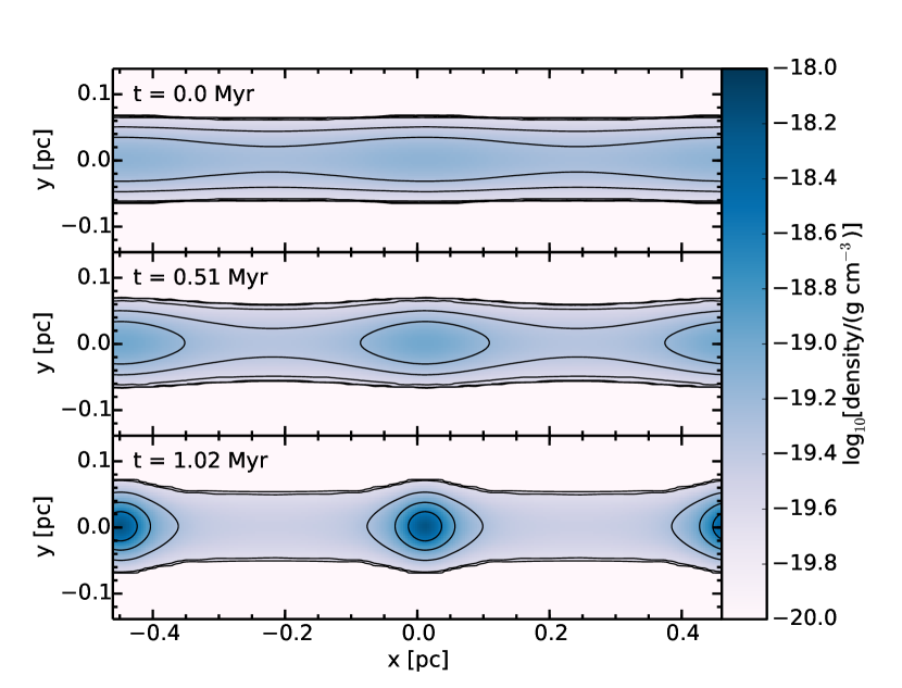
Figure 1: Density slice in the x-y plane through the center of the simulation of filament 2 in log-space. Only the filament gas is plotted ($\rho>10^{-20}\text{\,g cm${}^{-3}$}$). The upper panel shows the filament at the beginning which we define to be 1 Myr before the final state. The lower panel shows the final state that is compared with the observations. The timestep of the middle panel is exactly in between the two. The contours show equi-density levels normalized on the maximum density of the respective timestep and increase linearly in log-space to always show five contours. As one can see, the form of the emerging density clump changes from prolate in the linear evolution phase to becoming more and more roundish in the non-linear phase, a behavior which was also seen in SPH-simulations executed by Inutsuka & Miyama (1992).

The numerical simulations were executed with the RAMSES code (Teyssier, 2002). The code is capable of solving the discretised Euler equations in their conservative form on an Cartesian grid in 1D, 2D and 3D with a second-order Godunov scheme. For our simulation we used the MUSCL scheme (Monotonic Upstream-Centred Scheme for Conservation Laws, van Leer (1976)) in combination with the HLLC-Solver (Toro et al., 1994) and the multidimensional MC slope limiter (van Leer, 1979) was applied in order to achieve a total variation diminishing scheme. The gravity is solved using the built-in multigrid solver.

We place the filament axis in the x-direction of a 3D box and use periodic boundary conditions in this dimension in order to simulate an infinite filament. We set the boxsize to twice the dominant perturbation length in order to resolve it correctly and to stay close to the observations. The boundaries in perpendicular directions of the filament are set as outflow condition. The potential of the ghost cells has to be set to zero in order to not introduce a gravitational focus to the box center due to the mixed boundary conditions.

The filament gas is set to be isothermal with a temperature of 10 K and a molecular weight of $\mu=2.36$. The external gas surrounding the filament is fixed to be isobaric at all times and in pressure equilibrium with the boundary pressure of the filament:

$$P_{b}=\rho_{b}c_{s}^{2}$$ (11)

In order to minimize the effect of accretion we set the external density to a very low value of $10^{-4}$ times the filament boundary density. Real physical accretion would affect the growth of perturbations, but to quantify this is above the scope of this paper.

As the boxsize is larger than the filament diameter, we employ adaptive mesh refinement (AMR), which allows us to keep the resolution low in the low-density external gas. We enforce a refinement of the central region to give us an effective resolution of $256^{3}$ for the dense filament gas, which is enough to fulfill the Truelove criterion for the maximum occurring density within a factor of 16 at all times (Truelove et al., 1997) aside from the late core collapse in filament 2 where we still fulfill the Truelove criterion within a factor of 8. In order to check for consistency and rule out a limitation by resolution we also repeat the simulations with half the resolution and look for mayor differences between the results.

The density perturbation is set according to Equation 4 with a very small amplitude of 1% of the initial density, as the velocity has to adjust to the perturbed state. The phase of the density perturbation is set at random, but as the box is periodic in the direction of the filament axis, it has no influence on the solution.

5 Simulations

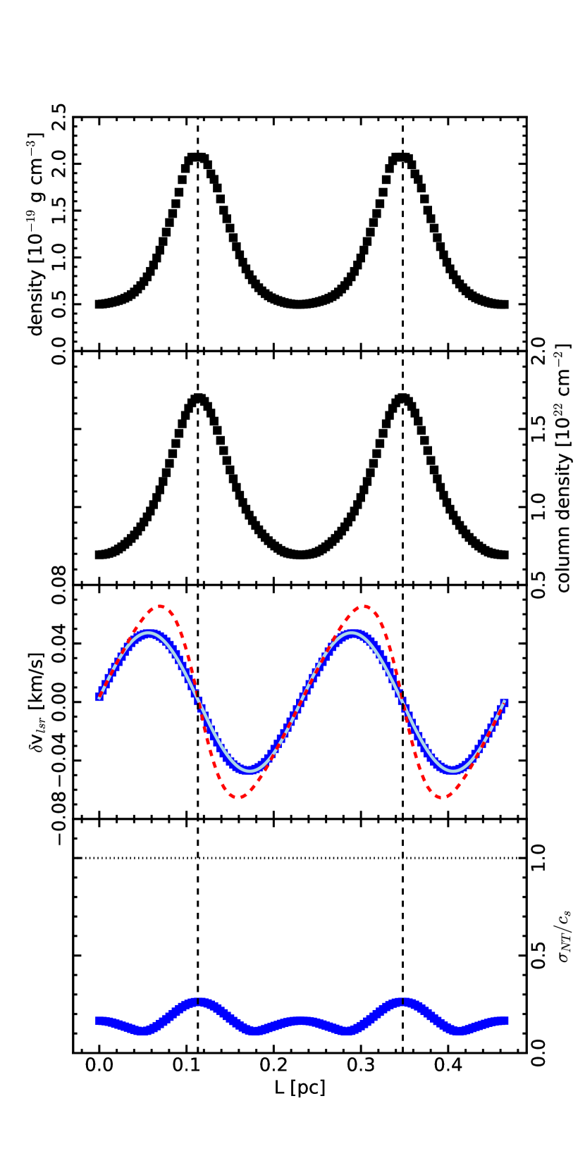
Figure 2: Results of the simulation for filament 1 in a line-of-sight projection of 57°along the axis of the filament. The upper panel shows the central volume density along the filament with two distinct cores also marked by the dashed, vertical lines. The density maximum and minimum matches the observation within a factor of two. The second panel shows the surface density summed up along the line-of-sight for a gas with a molecular weight of $\mu=2.36$. The third panel shows the velocity centroid variation as blue squares. Our fit to the data is given by the light blue line and the true projected central axis velocity is shown by the dashed, red line. As one can see, the true central velocity pattern is hidden with the maxima being damped by the velocity structure inside the filament. The velocity centroid pattern shows nearly the same amplitude of $0.05\text{ km s}^{-1}$ compared to the observed amplitude of $0.04\text{ km s}^{-1}$. The lower panel shows the non-thermal velocity dispersion in units of the sound speed. The dispersion is subsonic throughout with a mean value of $\left\langle\sigma_{\text{nt}}\right\rangle/c_{s}\approx 0.17$ which is about a third of what is observed in filament 1 ($\left\langle\sigma_{\text{nt}}\right\rangle/c_{s}=0.57\pm 0.15$ (Hacar & Tafalla, 2011)).

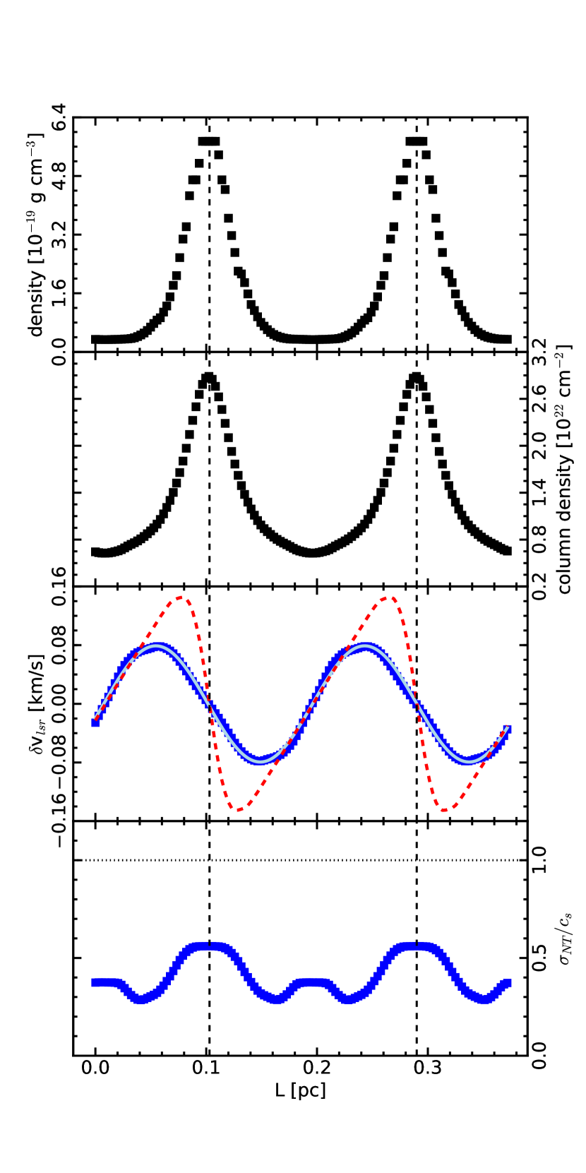
Figure 3: As in Figure 2 but for filament 2 in a line-of-sight projection of 66°. Again, the upper panel shows that the volume density matches the observation within a factor of two. The cores are more pronounced than for filament 1 and the volume density does not follow a sinusoidal pattern along the filament but shows a flat decreased density between the cores. This feature is harder to see in the surface density in the second panel. The amplitude of the velocity centroid variation is somewhat higher than the fit of the observations, $0.08\text{ km s}^{-1}$ compared to $0.04\text{ km s}^{-1}$, but the original observed velocity data of filament 2 does not follow a well defined sinusoidal curve (Hacar & Tafalla, 2011). The true central velocity structure is even more damped than in filament 1. It shows more pronounced slopes which indicates that matter from a broader region is pulled onto the density maxima. The non-thermal velocity dispersion in the lower panel is about twice that of the simulation of filament 1 with a mean value of $\left\langle\sigma_{\text{nt}}\right\rangle/c_{s}\approx 0.40$ which is around a factor of 1.5 lower compared to the observed value of $\left\langle\sigma_{\text{nt}}\right\rangle/c_{s}=0.63\pm 0.16$.

5.1 Comparison with the observation

We let the simulations run until the maximum density matches the observed central core density. An example of a simulation can be seen in Figure 1 where we plot a density slice through the center of the filament with overlaying density contours. The timescale is restricted by the lifetime of a molecular cloud, which is estimated to be of the order of a few Myr, especially for Taurus (Palla & Stahler, 2000; Hartmann, 2001; White & Ghez, 2001). It is therefore reasonable to assume 1 Myr as typical timescale for filament fragmentation. This timescale also coincides with the average lifetime of a core with typical densities of $10^{4}\text{ cm}^{-3}$ (Lee & Myers, 1999; Jessop & Ward-Thompson, 2000; Nakamura & Li, 2005), which serves as a good approximation for the total starless core phase. In our case, as the evolution should be effectively self-similar in the linear phase, the evolution timescale is then a function of the initial amplitude of the perturbation. Starting with a very small initial perturbation and running the simulation until the observed state is reached, allows us to actually determine the most likely initial amplitude as the perturbations strength reached one Myr before the finale state.

In order to compare our simulation result with the observations, we assume an inclination as described in subsection 3.2. We then use this inclination to determine the line-of-sight velocity distribution for each spatial pixel. In order to get the centroid velocity, we treat every volume element of the computational grid as an emitter of a discrete line-of-sight velocity value. These are converted to Gaussian line profiles with a dispersion of $\sigma=0.0526\text{ km s}^{-1}$, corresponding to the thermal linewidth of C¹⁸O, and are weighted with the respective density. The line profiles are binned into histograms with a bin width of $0.05\text{ km s}^{-1}$ in order to get a complete line emission for each observed spatial pixel and we measure the velocity centroid by fitting a Gaussian to the line, as an observer would do.

The result for our converged models is shown in Figure 2 for filament 1 and Figure 3 for filament 2 together with the central volume density, the column density in the line-of-sight and the non-thermal velocity dispersion of the Gaussian fit. Filament 1 has an unprojected wavelength of $0.43\text{ pc}$, an inclination angle of 57°and an initial line-mass of $f_{\text{cyl}}=0.51$. Filament 2 has an unprojected wavelength of $0.46\text{ pc}$, an inclination angle of 66°and an initial line-mass of $f_{\text{cyl}}=0.43$. The projected core distances of $0.23\text{ pc}$ and $0.19\text{ pc}$ respectively match the observed spacing and the maximum central volume densities of $2.07\cdot 10^{-19}\text{\,g cm${}^{-3}$}$ and $5.74\cdot 10^{-19}\text{\,g cm${}^{-3}$}$ also agree with the observations. The minimum of the central volume densities of $4.98\cdot 10^{-20}\text{\,g cm${}^{-3}$}$ and $3.37\cdot 10^{-20}\text{\,g cm${}^{-3}$}$ match the observed densities between the cores within a factor of two, which is the estimated error of measurement of Hacar & Tafalla (2011).

The spacial distribution of the line-of-sight centroid velocities is in good agreement with the observations. Especially filament 1 where the observed velocity data shows a sinusoidal curve with an amplitude of $0.04\text{ km s}^{-1}$ is well matched. Our fit, given by the solid light blue line, has an amplitude of $0.05\text{ km s}^{-1}$ but this is still within the measurement error of $0.01\text{ km s}^{-1}$. Hacar & Tafalla (2011) also fitted an amplitude of $0.04\text{ km s}^{-1}$ to the line-of-sight centroid velocity distribution of filament 2 but the observed velocity structure is ambiguous. The observed centroid velocity of filament 2 varies up to a value of $0.1\text{ km s}^{-1}$ and does not follow a sinusoidal pattern very well. Contrarily to the observation, we see a sinusoidal pattern in the centroid velocity variation. We find an amplitude about twice as large as the observed fit, namely $0.08\text{ km s}^{-1}$. Why the observed centroid velocity does not follow a clear pattern is not clear and could be due to more complex motions inside the filament. The velocity patterns of both filaments show a clear $\lambda/4$ shift in phase compared to the density perturbation, as they do in the observations, which is an indicator of the core-forming motions (Gehman et al., 1996).

The dashed, red lines in Figure 2 and Figure 3 show the true, inclination corrected, central axis velocity in longitude direction of the filament. Due to the central axis being the densest component, we would have expected that this velocity agrees with the projected line-of-sight velocity pattern as we only see weak radial infall motions in the majority of the filament. However, contrarily to our expectation, the true motion differs significantly from the line-of-sight velocity structure. Its maxima are large with a difference that is almost a factor of 2 in filament 2. In addition, the location of the maxima is shifted towards the clumps. In the strong non-linear case of filament 2 the true velocity pattern cannot be modeled well by a sinusoidal pattern. Interestingly, however, the projected velocity structure still resembles a sinusoidal pattern well.

The lowest panel shows the non-thermal velocity dispersion in the line of sight through the centre of the filament. It is calculated by measuring the FWHM, here denoted by $\Delta v$, of the Gaussian fit to the line-of-sight velocity data and by using the fact that the contribution of the thermal and non-thermal gas motions to the linewidth add in quadrature (e.g. Myers, 1983):

$$\sigma_{\text{nt}}=\sqrt{\frac{\Delta v^{2}}{8\ln 2}-\frac{k_{B}T}{m}}$$ (12)

where $m$ is the mass of the observed molecule, in this case C¹⁸O. We find that the gas is very subsonic throughout the filaments, with variations due to higher velocity dispersions inside and between the cores. We find that the higher velocity dispersion inside the cores is not only due to the radial collapse of the filament but is dominated by the infall of gas coming from the bulk of the filament. It is interesting to note that, although we do not model subsonic turbulence, the ordered motions inside the filament already lead to a considerable amount of non-thermal velocity dispersion. The mean of the dispersion in units of the sound speed is about $\left\langle\sigma_{\text{nt}}\right\rangle/c_{s}\approx 0.17$ for filament 1 and $\left\langle\sigma_{\text{nt}}\right\rangle/c_{s}\approx 0.40$ for filament 2. Comparing the modeled velocity dispersion to the observed values of $\left\langle\sigma_{\text{nt}}\right\rangle/c_{s}=0.57\pm 0.15$ and $\left\langle\sigma_{\text{nt}}\right\rangle/c_{s}=0.63\pm 0.16$ respecitvely and taking into account that velocity dispersions add in quadrature it becomes clear that in the case of the observations subsonic turbulence still dominates the non-thermal component of the velocity dispersion even with strong underlying ordered motion.

In the end, we find that the initial, unperturbed central density of the filaments was $8.2\cdot 10^{-20}\text{\,g cm${}^{-3}$}$ for filament 1 and $6.1\cdot 10^{-20}\text{\,g cm${}^{-3}$}$ for filament 2. Both lie considerably below the mean value of the maximum and minimum observed density of about $1.2\cdot 10^{-19}\text{\,g cm${}^{-3}$}$ for filament 1 and $2.9\cdot 10^{-19}\text{\,g cm${}^{-3}$}$ for filament 2. This signifies that there is a considerable amount of asymmetrical evolution where more mass is transferred to the density maxima than is taken from the density minima. This leads to an enhancement of the maximum density while leading to a slower density decrease between the cores. This effect is stronger in filament 2 than in filament 1 as can be seen from the bigger discrepancy of the initial central density and the observed density mean.

5.2 Dynamical evolution

In order to understand the asymmetrical evolution of the maximum and minimum density, we take a closer look at the time evolution of the perturbed quantities. Each perturbation of every variable should follow Equation 5. Thus, they should follow a linear evolution in log-space. This is shown for the central maximum density and central maximum velocity in the filament axis in Figure 4 for filament 1 and in Figure 5 for filament 2. In order to stay close to a reasonable limit of 1 Myr (see previous subsection), we start the evolution of filament 1 at about 10% perturbation strength and of filament 2 at about 20%. Both the maximum density and maximum velocity follow the linear prediction for the majority of the evolution with the density showing some oscillation around the linear prediction. In the late phase of the evolution, both filaments show a clear non-linear growth of the maximum density. It is worth noting that this non-linear phase is not short in the sense that all the mass of the filament collapses into a core in a fast period of time, but it is a smooth process, which can easily take up to 0.4 Myr or nearly half of the whole formation time of a core and still leaves diffuse gas to make up the filament. Also note that the velocity does not follow the same non-linear evolution initially. Only when we let the simulations run further, we see that the velocity follows with a delay of about 0.3 Myr. At that point in time, the cores are in a much more developed state and the simulations brake down due to resolution issues.

In order to have a deeper look into the non-linear phase we look at the line-mass in the slice of the maximum density. The line-mass of a pressure-bound filament is given by:

$$\frac{M}{L}=\int^{R}_{0}2\pi r\rho(r)dr$$ (13)

Inserting Equation 4, one can show, as the perturbation is independent of radius and the integration just gives the initial line-mass, that the time evolution is given by:

$$\left(\frac{M}{L}\right)(t)=\left(\frac{M}{L}\right)_{0}[1+\epsilon\exp(ikz-i\omega t)]$$ (14)

This indicates that, not only is there a redistribution of mass inside the filament, but that the line-mass also follows exactly the same evolution as the density.

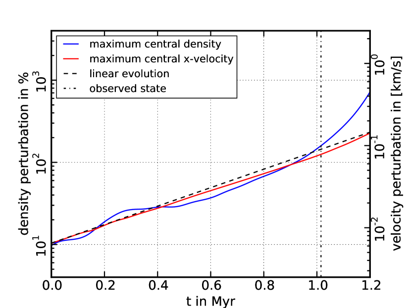
Figure 4: Evolution of the maximum central density (blue, left axis) and x-velocity (red, right axis) of filament 1. Both follow the analytic prediction until the density reaches a perturbation strength of about 100% where a non-linear evolution in density sets in. The dashed-dotted vertical line gives the point in time of the observation.

We plot the time evolution of the maximum density together with its respective line-mass ratio $f_{\text{cyl}}$ of filament 2 in Figure 6. The scale of $f_{\text{cyl}}$ is linear in order to see when the line-mass becomes supercritical. One can clearly see that $f_{\text{cyl}}$ exceeds 1.0 after about 0.85 Myr. This coincides more or less with the maximum central density entering the non-linear part of its evolution and dominates the late evolution. This indicates that the reason for the non-linear evolution of the maximum central density is that the region containing the cores are supercritical in the line-mass. This leads to a radial collapse of the filament at the position of the core as it cannot sustain hydrodynamical equilibrium which in turn enhances the central density.

This effect can account for the majority of the asymmetry but we also observe a reduced growth of the perturbation of the density minimum. In Figure 7 we plot the evolution of the maximum and the minimum density as well as the evolution of the maximum and minimum line-mass, both on a logarithmic scale to show the linear evolution. Note that, not only does the density follow the linear prediction but also the line-mass as predicted by Equation 14. One can also see the non-linear evolution of the maximum density in the line-mass maximum but it does not grow as fast as the density. As radial collapse of the filament would not lead to a difference in line-mass, this indicates that the density growth is not fed by radial collapse alone.

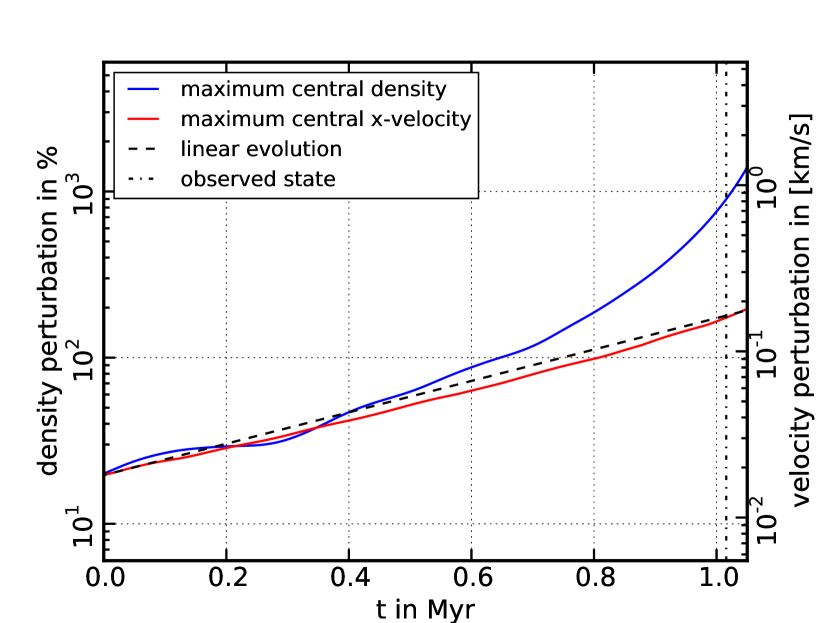
Figure 5: As in Figure 4, but for filament 2. Filament 2 shows the same evolutionary characteristics as filament 1, but in order to fulfill the time constraint of about 1 Myr, we need an initial density perturbation of around 20%. One can see that the observed state lies far deeper in the non-linear regime than for filament 1.

An interesting effect is that the evolution of the minimum density, as well as the minimum line-mass, flattens as the perturbation of the maximum becomes non-linear. This implies that the mass is not redistributed from the minimum to the maximum anymore but that the cores accrete mass from all over the bulk of the filament, which can be seen in the central volume density of filament 2 in Figure 3. The area between the cores shows a flat decreased density, with the cores being very pronounced and peaked, indicating that the cores also pull in mass from the filament axis. This means that as we approach the supercritical state of the cores, the accretion changes from a simple linear enhancement and reduction of the maximum and minimum respectively to a radial, spherical symmetric accretion onto the cores. This effect has also been shown and studied by Inutsuka & Miyama (1992) in SPH-simulations where they see the same behavior in the non-linear phase.

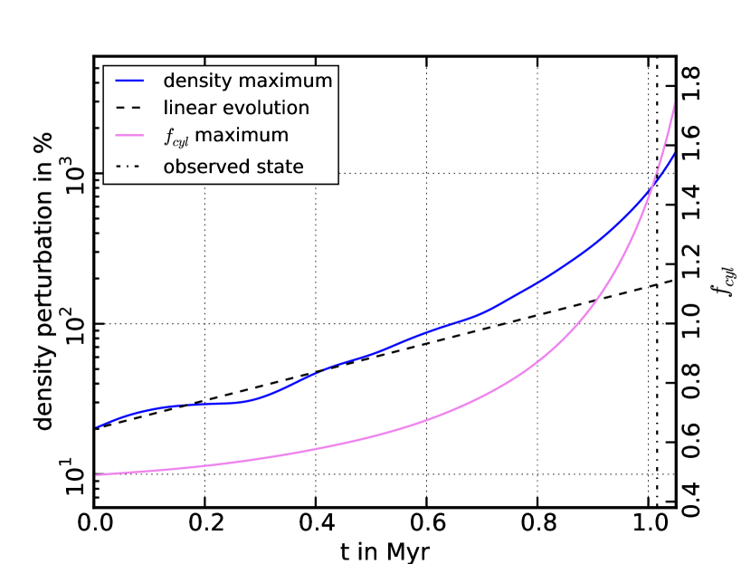
Figure 6: Evolution of the maximum density perturbation in log-space (blue, left axis, logarithmic scale) of filament 2 together with the evolution of $f_{\text{cyl}}$ (violet, right axis, linear scale) in the maximum density filament slice. One can see that the non-linear evolution of the maximum density is tied to the fact that the line-mass enters the critical regime ($f_{\text{cyl}}>1$). This means the maximum density evolution is driven primarily by the radial collapse of the filament in this section.

The change from linear to non-linear evolution also leads to a difference in core morphology and has an important implication for observed cores. This change can be seen in Figure 1 where the density contours show the cores initially forming to have a prolate shape, as matter is only transferred from the minimum to the maximum density. This changes drastically in the non-linear phase at the end of the simulation where the dense cores clearly show a generally round form in the density distribution. This was also seen in the simulations of Inutsuka & Miyama (1992) where the cores approached a near spherical form for late times in the non-linear phase. If one were to observe a dense core that displays an elongated, prolate form, it could be a strong hint that it is situated in the linear evolutionary phase. Indeed, observed cores typically show an elongated form (Benson & Myers, 1989) which is consistent with the fact that cores spend the bigger part of their lifetime in the linear evolutionary phase. However, it is obvious that there is an observational bias to detect dense cores which are likely to be in the non-linear phase already as they would not easily stand out of the filament gas otherwise. For instance, at the beginning of the non-linear phase of the simulation of filament 2 the cores only have an over-density of a factor of about two with respect to the filament gas.

The factor of two difference in the initial perturbation of the density maximum and the density minimum in Figure 7 stems from the fact that we start the simulation at an even earlier time with a very small perturbation strength in order to let the filament adjust to the perturbation. Although it is a relatively small difference, it highlights the fact that the density minimum already evolved slower than the density maximum. Starting with different values for the initial perturbation strength shows that the factor of two is robust and seems to be hard to avoid. Nevertheless, it is of relatively minor impact, since a factor two is also the inherent error in the observation and would not lead to an offset of the mean density as initial condition.

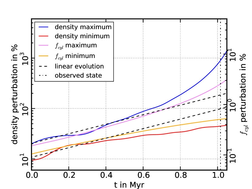
Figure 7: Evolution of the maximum and absolute minimum value of the density perturbation (left axis) of filament 2 together with the evolution of the absolute value of the perturbation in $f_{\text{cyl}}$ (right axis) in the respective filament slice. The minimum density perturbation evolves slower as predicted, growing even slower as time progresses. This means that the cores are not feeded symmetrically by the density minima, but accrete mass from over the whole filament.

5.3 External pressure

From Equation 8, it is possible to determine the boundary density of the filaments. This value can then be used in Equation 11 to get an estimate of the pressure of the surrounding material. Using our derived values of $\rho_{0}=8.18\cdot 10^{-20}\text{\,g cm${}^{-3}$}$ and $f_{\text{cyl}}=0.51$ for filament 1 and $\rho_{0}=6.12\cdot 10^{-20}\text{\,g cm${}^{-3}$}$ and $f_{\text{cyl}}=0.43$ for filament 2, both filaments give nearly the exact same value for the external pressure of $P_{\text{ext}}/k_{B}=5.01\cdot 10^{4}\text{\,K cm${}^{-3}$}$ and $P_{\text{ext}}/k_{B}=5.08\cdot 10^{4}\text{\,K cm${}^{-3}$}$ where $k_{B}$ is the Boltzmann constant. The consistency of both values could be a coincidence, but is reassuring and shows the power of the pressure truncated filament method to predict the environmental pressure.

However, the source of the external pressure is not clear and is open to debate. It is larger than the usually assumed total (thermal + turbulent) gas pressure of the interstellar medium, which is estimated to be of the order of $P_{\text{ISM}}/k_{B}\approx 10^{3}-10^{4}\text{\,K cm${}^{-3}$}$, e.g. by Bertoldi & McKee (1992), although they also estimate the gravitational pressure of the weight of the overlying material of different molecular clouds on cores and get values in a range of $P_{G}/k_{B}\approx 10^{4}-10^{5}\text{\,K cm${}^{-3}$}$. While this pressure is more important in quiescent clouds and not necessarily as high for turbulent clouds, gravitational pressure can add to the overall external pressure.

In addition, warm ionized gas can also lead to a supportive pressure, as has been shown for the Pipe Nebula (Gritschneder & Lin, 2012). They also determine pressure values in the range of $P_{\text{ion}}/k_{B}\approx 10^{4}-10^{5}\text{\,K cm${}^{-3}$}$. A possible source for ionizing radiation is AB Aurigae, which has been shown to heat the diffuse gas component while having nearly no influence on the dense gas (Duvert et al., 1986; Ladd & Myers, 1991). However, for the estimated environmental densities of order $5\cdot 10^{2}\text{ cm}^{-3}$ we would require a temperature of around 100 K which is not observed in the external medium.

Another source of external pressure is turbulent ram pressure $P_{\text{ram}}=\rho\sigma_{\text{turb}}^{2}$ where $\sigma_{\text{turb}}$ is calculated according to Equation 12. The relevant velocity dispersion $\sigma_{\text{turb}}$ for an external ram pressure is not the intrinsic velocity dispersion of the filaments but that of the whole region. The observations of Hacar & Tafalla (2011) show that the C¹⁸O gas is measured over the range of $\Delta v=1.2\text{ km s}^{-1}$. Assuming an external density of $\rho_{b}\sim 5\cdot 10^{2}\text{ cm}^{-3}$ leads to an external pressure of about $P_{\text{ram}}/k_{B}\approx 4\cdot 10^{4}\text{\,K cm${}^{-3}$}$ which is in excellent agreement with our external pressure estimate.

Although the source of the external pressure still remains unclear, a good candidate is therefore turbulent ram pressure. The theoretical model does not allow for a big leeway in the external pressure estimate and further observations are required to confirm this conjecture and determine the origin of the external pressure.

6 Discussion and conclusions

Even though we can reproduce the observational data well, some caveats remain. First and foremost, we simulate an infinite filament by using periodic boundary conditions. This is not a perfect representation of reality and our choice of boundary prevents the global collapse and edge-effects expected in finite filaments. A future study must include effects of a non-periodic boundary. It was shown by Clarke & Whitworth (2015) using semi-analytical methods and simulations that the global timescale for collapse of filaments with greater aspect ratios than $A>2$ is:

$$t_{\text{col}}=\frac{0.49+0.25A}{\sqrt{G\frac{(M/L)}{\pi R^{2}}}}$$ (15)

Using this formula, we find that the timescales for global collapse of our filaments are around 1.5 Myr. Thus, although fragmentation is physically possible, the filament will also change its form on a Myr scale. This will definitely influence fragmentation length- and timescales and if it is not possible to find other stabilizing processes, e.g. rotation or magnetic fields, this effect has to be taken into account.

Furthermore, although we can explain the observed densities, some differences to the observations remain. Most notably, the cores in Figure 2 and Figure 3 are more peaked than the observed cores. Also the observed filaments have a diameter of about 0.2 pc in contrast to our simulations where the filaments have a diameter of about 0.14 pc. The reason for this could be that we do not include the intrinsic turbulence. Hacar & Tafalla (2011) do find that a considerable amount of sub-sonic turbulence of about 0.5 times the sound speed dominates the filaments. This will naturally lead to puffed-up cores and a wider filament itself. Turbulence could indeed also change the form of the filament and fragmentation length- and timescales and is a factor to take into account but as it does not change the line-mass that regulates the fragmentation the impact should be relatively small. Still, a detailed study on the effect of turbulence would be interesting in order to understand better whether the fragmentation presented here is still possible.

Additionally, the observed cores are not symmetrical. For an idealized analysis we treat them as symmetric with a central density corresponding to their mean, but in reality their central density differs up to a factor of about three for filament 2. This could be either an effect of a clumpy or uneven initial mass distribution or of an asymmetrical evolution out of an evenly mass-distributed idealized filament. In an extended study, it should be possible to break their symmetrical evolution by introducing a power spectrum on the initial perturbation instead of only using the dominant wavelength.

Nevertheless, we have shown that the fragmentation length scale can indeed be explained by subsonic gravitational fragmentation of the filament, assuming an idealized model. Together with a constraint on the inclination we can estimate line-of-sight centroid velocity variations and compare them to the observations. Our models give the most likely properties to be:

Filament 1

• an unprojected length of 0.95 pc

• an inclination of 57°

• a line-mass of $f_{\text{cyl}}=0.51$

• an initial central density of $\rho_{0}=8.18\cdot 10^{-20}\text{\,g cm${}^{-3}$}$

• an external pressure of $P_{\text{ext}}/k_{B}=5.01\cdot 10^{4}\text{\,K cm${}^{-3}$}$

Filament 2

• an unprojected length of 1.03 pc

• an inclination of 66°

• a line-mass of $f_{\text{cyl}}=0.43$

• an initial central density of $\rho_{0}=6.12\cdot 10^{-20}\text{\,g cm${}^{-3}$}$

• an external pressure of $P_{\text{ext}}/k_{B}=5.08\cdot 10^{4}\text{\,K cm${}^{-3}$}$

Moreover, we demonstrated that cores can spend a considerable amount of their lifetime in a non-linear phase where their central density grows faster than a simple symmetrical mass transfer from the density minimum to the core. This is due to the fact that the densest regions of a filament exceed the line-mass where a radial hydrodynamic equilibrium is possible. This does not lead to an instant radial collapse, but the cores accrete matter radially, as well as from the whole filament. This makes them live long enough to be observed in the non-linear phase.

Most importantly, the change from linear to non-linear evolution is indicated in a change of core morphology. While a symmetrical redistribution of material from the minimum to maximum density leads to a prolate form, the radial collapse in all directions of the cores in the non-linear phase makes the core roundish in appearance. The high density contrasts from core to filament gas which are only achieved in the non-linear evolution makes cores more likely to be observed in the non-linear phase.

References

- André et al. (2010) André P., et al., 2010, A&A, 518, L102
- Arzoumanian et al. (2011) Arzoumanian D., et al., 2011, A&A, 529, L6
- Arzoumanian et al. (2013) Arzoumanian D., André P., Peretto N., Könyves V., 2013, A&A, 553, A119
- Bastien (1983) Bastien P., 1983, A&A, 119, 109
- Bastien et al. (1991) Bastien P., Arcoragi J.-P., Benz W., Bonnell I., Martel H., 1991, ApJ, 378, 255
- Benson & Myers (1989) Benson P. J., Myers P. C., 1989, ApJS, 71, 89
- Bertoldi & McKee (1992) Bertoldi F., McKee C. F., 1992, ApJ, 395, 140
- Burkert & Hartmann (2004) Burkert A., Hartmann L., 2004, ApJ, 616, 288
- Clarke & Whitworth (2015) Clarke S. D., Whitworth A. P., 2015, MNRAS, 449, 1819
- Duvert et al. (1986) Duvert G., Cernicharo J., Baudry A., 1986, A&A, 164, 349
- Evans et al. (2009) Evans II N. J., et al., 2009, ApJS, 181, 321
- Fiege & Pudritz (2000) Fiege J. D., Pudritz R. E., 2000, MNRAS, 311, 105
- Fischera & Martin (2012) Fischera J., Martin P. G., 2012, A&A, 542, A77
- Gehman et al. (1996) Gehman C. S., Adams F. C., Fatuzzo M., Watkins R., 1996, ApJ, 457, 718
- Gritschneder & Lin (2012) Gritschneder M., Lin D. N. C., 2012, ApJ, 754, L13
- Hacar & Tafalla (2011) Hacar A., Tafalla M., 2011, A&A, 533, A34
- Hacar et al. (2013) Hacar A., Tafalla M., Kauffmann J., Kovács A., 2013, A&A, 554, A55
- Hartmann (2001) Hartmann L., 2001, AJ, 121, 1030
- Heyer et al. (1987) Heyer M. H., Snell R. L., Goldsmith P. F., Myers P. C., 1987, ApJ, 321, 370
- Inutsuka & Miyama (1992) Inutsuka S.-I., Miyama S. M., 1992, ApJ, 388, 392
- Inutsuka & Miyama (1997) Inutsuka S.-i., Miyama S. M., 1997, ApJ, 480, 681
- Jessop & Ward-Thompson (2000) Jessop N. E., Ward-Thompson D., 2000, MNRAS, 311, 63
- Klessen et al. (2005) Klessen R. S., Ballesteros-Paredes J., Vázquez-Semadeni E., Durán-Rojas C., 2005, ApJ, 620, 786
- Ladd & Myers (1991) Ladd E. F., Myers P. C., 1991, in Haschick A. D., Ho P. T. P., eds, Astronomical Society of the Pacific Conference Series Vol. 16, Atoms, Ions and Molecules: New Results in Spectral Line Astrophysics. p. 241
- Larson (1985) Larson R. B., 1985, MNRAS, 214, 379
- Lee & Myers (1999) Lee C. W., Myers P. C., 1999, ApJS, 123, 233
- Moeckel & Burkert (2015) Moeckel N., Burkert A., 2015, ApJ, 807, 67
- Molinari et al. (2010) Molinari S., et al., 2010, A&A, 518, L100
- Myers (1983) Myers P. C., 1983, ApJ, 270, 105
- Nachman (1979) Nachman P., 1979, ApJS, 39, 103
- Nagasawa (1987) Nagasawa M., 1987, Progress of Theoretical Physics, 77, 635
- Nakamura & Li (2005) Nakamura F., Li Z.-Y., 2005, ApJ, 631, 411
- Nakamura et al. (1993) Nakamura F., Hanawa T., Nakano T., 1993, PASJ, 45, 551
- Ostriker (1964) Ostriker J., 1964, ApJ, 140, 1056
- Padoan et al. (2001) Padoan P., Juvela M., Goodman A. A., Nordlund Å., 2001, ApJ, 553, 227
- Palla & Stahler (2000) Palla F., Stahler S. W., 2000, ApJ, 540, 255
- Palmeirim et al. (2013) Palmeirim P., et al., 2013, A&A, 550, A38
- Pon et al. (2012) Pon A., Toalá J. A., Johnstone D., Vázquez-Semadeni E., Heitsch F., Gómez G. C., 2012, ApJ, 756, 145
- Recchi et al. (2013) Recchi S., Hacar A., Palestini A., 2013, A&A, 558, A27
- Schneider & Elmegreen (1979) Schneider S., Elmegreen B. G., 1979, ApJS, 41, 87
- Schneider et al. (2012) Schneider N., et al., 2012, A&A, 540, L11
- Shu et al. (1987) Shu F. H., Adams F. C., Lizano S., 1987, ARA&A, 25, 23
- Smith et al. (2016) Smith R. J., Glover S. C. O., Klessen R. S., Fuller G. A., 2016, MNRAS, 455, 3640
- Stodólkiewicz (1963) Stodólkiewicz J. S., 1963, Acta Astron., 13, 30
- Tafalla & Hacar (2015) Tafalla M., Hacar A., 2015, A&A, 574, A104
- Tafalla et al. (2004) Tafalla M., Myers P. C., Caselli P., Walmsley C. M., 2004, A&A, 416, 191
- Tafalla et al. (2006) Tafalla M., Santiago-García J., Myers P. C., Caselli P., Walmsley C. M., Crapsi A., 2006, A&A, 455, 577
- Tanaka et al. (2013) Tanaka T., et al., 2013, ApJ, 778, 34
- Teyssier (2002) Teyssier R., 2002, A&A, 385, 337
- Toro et al. (1994) Toro E., Spruce M., Speares W., 1994, Shock Waves, 4, 25
- Truelove et al. (1997) Truelove J. K., Klein R. I., McKee C. F., Holliman II J. H., Howell L. H., Greenough J. A., 1997, ApJ, 489, L179
- Vázquez-Semadeni et al. (2005) Vázquez-Semadeni E., Kim J., Shadmehri M., Ballesteros-Paredes J., 2005, ApJ, 618, 344
- White & Ghez (2001) White R. J., Ghez A. M., 2001, ApJ, 556, 265
- di Francesco et al. (2007) di Francesco J., Evans II N. J., Caselli P., Myers P. C., Shirley Y., Aikawa Y., Tafalla M., 2007, Protostars and Planets V, pp 17–32
- van Leer (1976) van Leer B., 1976, in Biskamp D., ed., Computing in Plasma Physics and Astrophysics. p. 1
- van Leer (1979) van Leer B., 1979, Journal of Computational Physics, 32, 101
- van den Ancker et al. (1998) van den Ancker M. E., de Winter D., Tjin A Djie H. R. E., 1998, A&A, 330, 145