An Efficient Algorithm for Periodic Riccati Equation for Spacecraft Attitude Control Using Magnetic Torques

Abstract

Spacecraft attitude control using only magnetic torques is a periodic time-varying system as the Earth magnetic field in the spacecraft body frame changes periodically while the spacecraft circles around the Earth. The optimal controller design therefore involves the solutions of the periodic Riccati differential or algebraic equations. This paper proposes an efficient algorithm for the periodic discrete-time Riccati equation arising from a linear periodic time-varying system $({\bf A},{\bf B})$, which explores and utilizes the fact that ${\bf A}$ is time-invariant and only ${\bf B}$ is time-varying in the system, a special properties associated with the problem of spacecraft attitude control using only magnetic torques.

Keywords: Periodic Riccati equation, spacecraft, attitude control, magnetic torque.

1 Introduction

SPACECRAFT attitude control using only magnetic torques has several attractive features, such as low cost, high reliability (without moving mechanical parts), and seamless implementation. Therefore, numerous research papers were focused on the problem of spacecraft attitude control using only magnetic torques in the last twenty five years (see [1, 2, 3, 4, 5, 6, 7, 8, 9, 10, 11, 12] and references therein). Because the Earth’s magnetic field in the spacecraft body frame is approximately a periodic function as the spacecraft circles around the Earth, the controller design should be based on a time-varying system. Therefore, state space model is a natural choice.

Some researchers [5, 6, 7] proposed direct design methods using Lyapunov stabilization theory. These designs use the nonlinear periodic model. The existence of the solutions for these designs implicitly depends on the controllability for the nonlinear time-varying system. Therefore, Bhat [13] investigated controllability of the nonlinear time-varying systems. However, the condition for the controllability of the nonlinear time-varying systems established in [13] is hard to be verified and is a sufficient condition. In addition, there is no systematic method for the selection of Lyapunov functions. Moreover, these designs do no consider the closed-loop system performances other than the stability.

A more realistic design strategy is to use linearized time-varying system models. The standard design methods for these models such as linear quadratic regulator (LQR) [1, 2, 3, 4, 10, 9, 11] and ${\bf H}_{\infty}$ control [12] are discussed. But two important issues were not addressed in these papers. First, the existence of the solutions of LQR and ${\bf H}_{\infty}$ control directly depends on the controllability (or a slightly weak condition named stabilizability) of the linear time-varying system which was not established for the spacecraft attitude control system using only magnetic torques. Second, the features and the structure of the spacecraft attitude control using magnetic torque were not explored. Instead, algorithms designed for general linear time-varying systems were used for this very specific problem. Therefore, those algorithms are not optimized for this problem.

The first issue is recently addressed in [14] in which the conditions for the controllability of spacecraft attitude control using only magnetic torques were established. The second issue is the focus of this paper, we will explore the features and structure of the problem and propose an efficient algorithm for the design of spacecraft attitude control using only magnetic torques.

There are two popular types of models used in spacecraft control system designs. Some of the designs adopted Euler angle models [1, 2, 3, 4, 10] but others used the reduced quaternion models [9, 11, 12]. We will adopt a reduced quaternion model because of the merits of the reduced quaternion model discussed in [15, 16, 17].

The remainder of the paper is organized as follows. Section 2 provides a description of the linear time-varying model of the spacecraft attitude control system using only magnetic torque. Section 3 derives the controller design algorithm for the linear time-varying system. Section 4 presents a simulation example to demonstrate the effectiveness and efficiency of the design algorithm. The conclusions are summarized in Section 5.

2 Spacecraft Model

The linearized continuous-time model for spacecraft attitude control using only magnetic torques can be expressed in a reduced quaternion form. Let ${\bf J}$ be the inertia matrix of a spacecraft defined by

$${\bf J}=\left[\begin{array}[]{ccc}J_{11}&J_{12}&J_{13}\\ J_{21}&J_{22}&J_{23}\\ J_{31}&J_{32}&J_{33}\end{array}\right].$$ (4)

We will consider the nadir pointing spacecraft. Therefore, the attitude of the spacecraft is represented by the rotation of the spacecraft body frame relative to the local vertical and local horizontal (LVLH) frame. Let ${\omega}=[\omega_{1},\omega_{2},\omega_{3}]^{{\rm T}}$ be the body rate with respect to the LVLH frame represented in the body frame, $\omega_{0}$ be the orbit (and LVLH frame) rate with respect to the inertial frame, represented in the LVLH frame. Let $\bar{{\bf q}}=[q_{0},q_{1},q_{2},q_{3}]^{{\rm T}}=[q_{0},{\bf q}^{{\rm T}}]^{{\rm T}}=[\cos(\frac{\alpha}{2}),\hat{{\bf e}}^{{\rm T}}\sin(\frac{\alpha}{2})]^{{\rm T}}$ be the quaternion representing the rotation of the body frame relative to the LVLH frame, where $\hat{{\bf e}}$ is the unit length rotational axis and $\alpha$ is the rotation angle about $\hat{{\bf e}}$. The control torques generated by magnetic coils interacting with the Earth’s magnetic field is given by (see [18])

$${\bf u}={\bf m}\times{\bf b}$$

where the Earth’s magnetic field in spacecraft coordinates, ${\bf b}(t)=[b_{1}(t),b_{2}(t),b_{3}(t)]^{{\rm T}}$, is computed using the spacecraft position, the spacecraft attitude, and a spherical harmonic model of the Earth’s magnetic field [19]; and ${\bf m}=[m_{1},m_{2},m_{3}]^{{\rm T}}$ is the spacecraft magnetic coils’ induced magnetic moment in the spacecraft coordinates. The time-variation of the system is an approximate periodic function of ${\bf b}(t)={\bf b}(t+P)$ where the orbital period is given by [18]

$$P=\frac{2\pi}{\omega_{0}}=2\pi\sqrt{\frac{a^{3}}{GM}},$$ (5)

where $a$ is the orbital radius (for circular orbit) and $GM=3.986005*10^{14}{m^{3}/s^{2}}$ [19]. This magnetic field ${\bf b}(t)$ can be approximately expressed as follows [4]:

$$\left[\begin{array}[]{c}b_{1}(t)\\ b_{2}(t)\\ b_{3}(t)\end{array}\right]=\frac{\mu_{f}}{a^{3}}\left[\begin{array}[]{c}\cos(\omega_{0}t)\sin(i_{m})\\ -\cos(i_{m})\\ 2\sin(\omega_{0}t)\sin(i_{m})\end{array}\right],$$ (6)

where $i_{m}$ is the inclination of the spacecraft orbit with respect to the magnetic equator, $\mu_{f}=7.9\times 10^{15}$ Wb-m is the field’s dipole strength. The time $t=0$ is measured at the ascending-node crossing of the magnetic equator. Then, the reduced quaternion linear time-varying system is given as follows [14]:

$$\left[\begin{array}[]{c}\dot{q}_{1}\\ \dot{q}_{2}\\ \dot{q}_{3}\\ \dot{\omega}_{1}\\ \dot{\omega}_{2}\\ \dot{\omega}_{3}\end{array}\right] = \left[\begin{array}[]{cccccc}0&0&0&.5&0&0\\ 0&0&0&0&.5&0\\ 0&0&0&0&0&.5\\ f_{41}&0&0&0&0&f_{46}\\ 0&f_{52}&0&0&0&0\\ 0&0&f_{63}&f_{64}&0&0\end{array}\right]\left[\begin{array}[]{c}{q}_{1}\\ {q}_{2}\\ {q}_{3}\\ {\omega}_{1}\\ {\omega}_{2}\\ {\omega}_{3}\end{array}\right]+\left[\begin{array}[]{ccc}0&0&0\\ 0&0&0\\ 0&0&0\\ 0&\frac{b_{3}(t)}{J_{11}}&-\frac{b_{2}(t)}{J_{11}}\\ -\frac{b_{3}(t)}{J_{22}}&0&\frac{b_{1}(t)}{J_{22}}\\ \frac{b_{2}(t)}{J_{33}}&-\frac{b_{1}(t)}{J_{33}}&0\end{array}\right]\left[\begin{array}[]{c}{m}_{1}\\ {m}_{2}\\ {m}_{3}\end{array}\right]$$ (34)

$$:= \left[\begin{array}[]{cc}{\bf 0}_{3}&\frac{1}{2}{\bf I}_{3}\\ \boldsymbol{\Lambda}_{1}&\boldsymbol{\Sigma}_{1}\end{array}\right]\left[\begin{array}[]{c}{\bf q}\\ \boldsymbol{\omega}\end{array}\right]+\left[\begin{array}[]{c}{\bf 0}_{3}\\ {\bf B}_{2}(t)\end{array}\right]{\bf m}={\bf A}{\bf x}+{\bf B}(t){\bf m},$$ (41)

where

$${\bf A}=\left[\begin{array}[]{cc}{\bf 0}_{3}&\frac{1}{2}{\bf I}_{3}\\ \boldsymbol{\Lambda}_{1}&\boldsymbol{\Sigma}_{1}\end{array}\right],\hskip 7.22743pt {\bf B}=\left[\begin{array}[]{c}{\bf 0}_{3}\\ {\bf B}_{2}(t)\end{array}\right],$$ (46)

$${\bf B}_{2}(t)=\left[\begin{array}[]{ccc}0&b_{42}(t)&b_{43}(t)\\ b_{51}(t)&0&b_{53}(t)\\ b_{61}(t)&b_{62}(t)&0\end{array}\right],$$ (47)

$$f_{41}=[8(J_{33}-J_{22})\omega_{0}^{2}]/J_{11}$$ (48)

$$f_{46}=(-J_{11}+J_{22}-J_{33})\omega_{0}/J_{11}$$ (49)

$$f_{64}=(J_{11}-J_{22}+J_{33})\omega_{0}/J_{33}$$ (50)

$$f_{52}=[6(J_{33}-J_{11})\omega_{0}^{2}]/J_{22}$$ (51)

$$f_{63}=[2(J_{11}-J_{22})\omega_{0}^{2}]/J_{33}$$ (52)

and

$$b_{42}(t)=\frac{2\mu_{f}}{a^{3}J_{11}}\sin(i_{m})\sin(\omega_{0}t)$$ (53)

$$b_{43}(t)=\frac{\mu_{f}}{a^{3}J_{11}}\cos(i_{m})$$ (54)

$$b_{53}(t)=\frac{\mu_{f}}{a^{3}J_{22}}\sin(i_{m})\cos(\omega_{0}t)$$ (55)

$$b_{51}(t)=-\frac{2\mu_{f}}{a^{3}J_{22}}\sin(i_{m})\sin(\omega_{0}t)=-b_{42}\frac{J_{11}}{J_{22}}$$ (56)

$$b_{61}(t)=-\frac{\mu_{f}}{a^{3}J_{33}}\cos(i_{m})=-b_{43}\frac{J_{11}}{J_{33}}$$ (57)

$$b_{62}(t)=-\frac{\mu_{f}}{a^{3}J_{33}}\sin(i_{m})\cos(\omega_{0}t)=-b_{53}\frac{J_{22}}{J_{33}}.$$ (58)

It is easy to verify that $\det{{\bf A}}=(\frac{1}{2})^{3}\det(\boldsymbol{\Lambda}_{1})$ and ${\bf A}$ is nonsingular if $J_{11}\neq J_{22}$, $J_{11}\neq J_{33}$, and $J_{33}\neq J_{22}$.

Oftentimes, a spacecraft controller is implemented in a computer system which is a discrete system. Therefore, the following discrete model is used for the design in practical implementation:

$${\bf x}_{k+1}={\bf A}_{k}{\bf x}_{k}+{\bf B}_{k}{\bf m}_{k}.$$ (59)

The system matrices $({\bf A}_{k},{\bf B}_{k})$ in the discrete model can be derived from (41), (46), and (47) by different methods. Let $t_{s}$ be the sample time, we use the following formulations.

$${\bf A}_{k}=({\bf I}+{\bf A}t_{s}),\hskip 7.22743pt{\bf B}_{k}={\bf B}(kt_{s})t_{s}.$$ (60)

Note that

$$\det({\bf I}+{\bf A}t_{s})=\det\left[\begin{array}[]{ccc}{\bf I}&&0.5t_{s}{\bf I}\\ t_{s}\boldsymbol{\Lambda}_{1}&&{\bf I}+t_{s}\boldsymbol{\Sigma}_{1}\end{array}\right]=\det\left[\begin{array}[]{ccc}{\bf I}&&0.5t_{s}{\bf I}\\ {\bf 0}_{3}&&{\bf I}+t_{s}\boldsymbol{\Sigma}_{1}-0.5t_{s}^{2}\boldsymbol{\Lambda}_{1}\end{array}\right]$$

which is invertiable as long as $t_{s}$ is selected small enough. It is worthwhile to mention that in both continuous-time and discrete-time models, the time-varying feature is introduced by time-varying matrices ${\bf B}(t)$ or ${\bf B}_{k}$; the system matrices ${\bf A}$ and ${\bf A}_{k}$ are constants and invertiable which are important for us to derive an efficient computational algorithm.

3 Computational Algorithm for the LQR Design

It is well-known that the LQR design relies on the solution of either the differential Riccati equation (for continuous-time systems) or the discrete Riccati equation (for discrete-time systems) [20]. If a system is periodic, such as (41) or (59), the LQR design relies on the periodic solution of the periodic Riccati equation [21]. Our discussion about the computational algorithm is focused on the solution of periodic discrete Riccati equation using the special properties of (59), i.e., ${\bf A}_{k}$ is constant and invertiable for $\forall k$.

3.1 Preliminary Results

Let

$${\bf L}=\left[\begin{array}[]{rclc}{\bf 0}&&{\bf I}&\\ -{\bf I}&&{\bf 0}&\end{array}\right]\in{\bf R}^{2n\times 2n},$$ (61)

where $n$ is the dimension of ${\bf A}$ or ${\bf A}_{k}$ in general case and $n=6$ in (41) and (59). Note that ${\bf L}^{{\rm T}}={\bf L}^{-1}=-{\bf L}$. Two types of matrices defined below are important to the solutions of the Riccati equations.

Definition 3.1 ([22])

A matrix ${\bf M}\in{\bf R}^{2n\times 2n}$ is Hamiltonian if ${\bf L}^{-1}{\bf M}^{{\rm T}}{\bf L}=-{\bf M}$. A matrix ${\bf M}\in{\bf R}^{2n\times 2n}$ is symplectic if ${\bf L}^{-1}{\bf M}^{{\rm T}}{\bf L}={\bf M}^{-1}$.

Proposition 3.1

If ${\bf M}_{1}$ and ${\bf M}_{2}$ are symplectic, then ${\bf M}_{1}{\bf M}_{2}$ is symplectic.

• Since ${\bf L}^{-1}{\bf M}_{1}^{{\rm T}}{\bf L}={\bf M}_{1}^{-1}$ and ${\bf L}^{-1}{\bf M}_{2}^{{\rm T}}{\bf L}={\bf M}_{2}^{-1}$, we have

  $$\begin{array}[]{cc}{\bf L}^{-1}({\bf M}_{1}{\bf M}_{2})^{{\rm T}}{\bf L}={\bf L}^{-1}{\bf M}_{2}^{{\rm T}}{\bf M}_{1}^{{\rm T}}{\bf L}={\bf L}^{-1}{\bf M}_{2}^{{\rm T}}{\bf L}{\bf L}^{-1}{\bf M}_{1}^{{\rm T}}{\bf L}={\bf M}_{2}^{-1}{\bf M}_{1}^{-1}=({\bf M}_{1}{\bf M}_{2})^{-1}.\end{array}$$

  This concludes the proof.       

In the sequel, we use $\lambda({\bf M})$ or simply $\lambda$ for an eigenvalue of a matrix ${\bf M}$ and $\sigma({\bf M})$ for the set of all eigenvalues of ${\bf M}$. The following two theorems play essential roles.

Theorem 3.1 ([23, 24])

Let ${\bf M}\in{\bf R}^{2n\times 2n}$ is Hamiltonian. Then $\lambda\in\sigma({\bf M})$ implies $-\lambda\in\sigma({\bf M})$ with the same multiplicity. Let ${\bf M}\in{\bf R}^{2n\times 2n}$ is symplectic. Then $\lambda\in\sigma({\bf M})$ implies $\frac{1}{\lambda}\in\sigma({\bf M})$ with the same multiplicity.

Theorem 3.2 ([25])

Let ${\bf M}\in{\bf R}^{n\times n}$. Then there exists an orthogonal similarity transformation ${\bf U}$ such that ${\bf U}^{{\rm T}}{\bf M}{\bf U}$ is quasi-upper-triangular. Moreover, ${\bf U}$ can be chosen such that the $2\times 2$ and $1\times 1$ diagonal blocks appear in any desired order.

Theorem 3.2 is the so called real Schur decomposition. Combining the above two theorems, we conclude that

Corollary 3.1

Let ${\bf M}\in{\bf R}^{2n\times 2n}$ is Hamiltonian or symplectic. Then there exists an orthogonal similarity transformation ${\bf U}$ such that

$$\left[\begin{array}[]{cc}{\bf U}_{11}&{\bf U}_{12}\\ {\bf U}_{21}&{\bf U}_{22}\end{array}\right]^{{\rm T}}{\bf M}\left[\begin{array}[]{cc}{\bf U}_{11}&{\bf U}_{12}\\ {\bf U}_{21}&{\bf U}_{22}\end{array}\right]=\left[\begin{array}[]{cc}{\bf S}_{11}&{\bf S}_{12}\\ {\bf 0}&{\bf S}_{22}\end{array}\right]$$ (62)

where ${\bf U}_{11},{\bf U}_{12},{\bf U}_{21},{\bf U}_{22},{\bf S}_{11},{\bf S}_{12},{\bf S}_{22}\in{\bf R}^{n\times n}$, and ${\bf S}_{11}$, ${\bf S}_{22}$ are quasi-upper-triangular. Moreover,

• if ${\bf M}$ is Hamiltonian, then $\sigma({\bf S}_{11})\leq 0$ (or $\sigma({\bf S}_{22})\geq 0$) and $\sigma({\bf S}_{22})\geq 0$ (or $\sigma({\bf S}_{11})\leq 0$).

• if ${\bf M}$ is symplectic, then $\sigma({\bf S}_{11})$ lies inside (or outside) the unit circle and $\sigma({\bf S}_{22})$ lies outside (or inside) the unit circle.

The Hamiltonian matrix is used in the derivation of the solution for the continuous-time differential Riccati equation, while the symplectic matrix is used in the derivation of the solution for the discrete-time algebraic Riccati equation. In our discussion, therefore, the symplectic matrix plays a fundamental role.

3.2 Solution of the Riccati Algebraic Equation

For a discrete linear time-varying system (59), the LQR state feedback control is to find the optimal ${\bf m}_{k}$ to minimize the following quadratic cost function

$$\lim_{N\rightarrow\infty}\left(\min\frac{1}{2}{\bf x}_{N}^{{\rm T}}{\bf Q}_{N}{\bf x}_{N}+\frac{1}{2}\sum_{k=0}^{N-1}{\bf x}_{k}^{{\rm T}}{\bf Q}_{k}{\bf x}_{k}+{\bf m}_{k}^{{\rm T}}{\bf R}_{k}{\bf m}_{k}\right)$$ (63)

where

$${\bf Q}_{k}\geq 0,$$ (64)

$${\bf R}_{k}>0,$$ (65)

and the initial condition ${\bf x}_{0}$ is given. The controllability of spacecraft attitude control using only magnetic torques is discussed in [14]. Therefore, if $({\bf A}_{k},{\bf Q}_{k})$ is detectable or ${\bf Q}_{k}>0$, the optimal feedback ${\bf m}_{k}$ is given by [20, 26]

$${\bf m}_{k}=-({\bf R}_{k}+{\bf B}_{k}^{{\rm T}}{\bf P}_{k+1}{\bf B}_{k})^{-1}{\bf B}^{{\rm T}}_{k}{\bf P}_{k+1}{\bf A}_{k}{\bf x}_{k},$$ (66)

where ${\bf P}_{k}$ is the unique positive semi-definite solution of the following discrete Riccati equation [20, 22, 26]

$${\bf P}_{k}={\bf Q}_{k}+{\bf A}^{{\rm T}}_{k}{\bf P}_{k+1}{\bf A}_{k}-{\bf A}_{k}^{{\rm T}}{\bf P}_{k+1}{\bf B}_{k}({\bf R}_{k}+{\bf B}_{k}^{{\rm T}}{\bf P}_{k+1}{\bf B}_{k})^{-1}{\bf B}_{k}^{{\rm T}}{\bf P}_{k+1}{\bf A}_{k},$$ (67)

with the boundary condition ${\bf P}_{N}={\bf Q}_{N}$. For this discrete Riccati equation (not necessarily periodic) given as (67), it can be solved using a symplectic system associated with (59) and (63) as follows [22, 26, 27].

$${\bf E}_{k}{\bf z}_{k+1}={\bf E}_{k}\left[\begin{array}[]{c}{\bf x}_{k+1}\\ {\bf y}_{k+1}\end{array}\right]={\bf F}_{k}\left[\begin{array}[]{c}{\bf x}_{k}\\ {\bf y}_{k}\end{array}\right]={\bf F}_{k}{\bf z}_{k}$$ (68)

where ${\bf x}_{k}$ is the state and ${\bf y}_{k}$ is the costate,

$${\bf E}_{k}=\left[\begin{array}[]{cc}{\bf I}&{\bf B}_{k}{\bf R}_{k}^{-1}{\bf B}_{k}^{{\rm T}}\\ {\bf 0}&{\bf A}_{k}^{{\rm T}}\end{array}\right],$$ (69)

$${\bf F}_{k}=\left[\begin{array}[]{cc}{\bf A}_{k}&{\bf 0}\\ -{\bf Q}_{k}&{\bf I}\end{array}\right].$$ (70)

If ${\bf E}_{k}$ is invertiable which is true for $\det({\bf I}+t_{s}\boldsymbol{\Sigma}_{1}-\frac{1}{2}t_{s}^{2}\boldsymbol{\Lambda}_{1})\neq 0$,

$${\bf E}_{k}^{-1}=\left[\begin{array}[]{cc}{\bf I}&-{\bf B}_{k}{\bf R}_{k}^{-1}{\bf B}_{k}^{{\rm T}}{\bf A}_{k}^{-{\rm T}}\\ {\bf 0}&{\bf A}^{-{\rm T}}_{k}\end{array}\right],$$

a symplectic matrix can be formed [27] as

$${\bf Z} = {\bf E}^{-1}_{k}{\bf F}_{k}=\left[\begin{array}[]{cc}{\bf I}&-{\bf B}_{k}{\bf R}_{k}^{-1}{\bf B}_{k}^{{\rm T}}{\bf A}_{k}^{-{\rm T}}\\ {\bf 0}&{\bf A}^{-{\rm T}}_{k}\end{array}\right]\left[\begin{array}[]{cc}{\bf A}_{k}&{\bf 0}\\ -{\bf Q}_{k}&{\bf I}\end{array}\right]$$ (75)

$$= \left[\begin{array}[]{cc}{\bf A}_{k}+{\bf B}_{k}{\bf R}_{k}^{-1}{\bf B}_{k}^{{\rm T}}{\bf A}_{k}^{-{\rm T}}{\bf Q}_{k}&-{\bf B}_{k}{\bf R}_{k}^{-1}{\bf B}_{k}^{{\rm T}}{\bf A}_{k}^{-{\rm T}}\\ -{\bf A}_{k}^{-{\rm T}}{\bf Q}_{k}&{\bf A}_{k}^{-{\rm T}}\end{array}\right].$$ (78)

It is straghtforward to verify that ${\bf L}^{-1}{\bf Z}^{{\rm T}}{\bf L}={\bf Z}^{-1}$, therefore, from Corollary 3.1, there exists an orthogonal matrix ${\bf U}$ such that

$$\left[\begin{array}[]{cc}{\bf U}_{11}&{\bf U}_{12}\\ {\bf U}_{21}&{\bf U}_{22}\end{array}\right]^{{\rm T}}{\bf Z}\left[\begin{array}[]{cc}{\bf U}_{11}&{\bf U}_{12}\\ {\bf U}_{21}&{\bf U}_{22}\end{array}\right]=\left[\begin{array}[]{cc}{\bf S}_{11}&{\bf S}_{12}\\ {\bf 0}&{\bf S}_{22}\end{array}\right].$$ (79)

The (steady state) solution of (67) is given as follows [22, Theorem 6].

Theorem 3.3

${\bf U}_{11}$ is invertiale and ${\bf P}={\bf U}_{12}{\bf U}_{11}^{-1}$ solves (67) with ${\bf P}={\bf P}^{{\rm T}}\geq 0$;

$$\sigma({\bf S}_{11}) = \sigma({\bf A}_{l}-{\bf B}_{k}({\bf R}_{k}+{\bf B}_{k}^{{\rm T}}{\bf P}_{k}{\bf B}_{k})^{-1}{\bf B}_{k}^{{\rm T}}{\bf P}_{k}{\bf A}_{k})$$ (80)

$$= \sigma({\bf A}_{k}-{\bf B}_{k}{\bf R}_{k}^{-1}{\bf B}_{k}^{{\rm T}}{\bf A}_{k}^{-{\rm T}}({\bf P}_{k}-{\bf Q}_{k}))$$

$$= \sigma({\bf A}_{k}-{\bf B}_{k}{\bf R}_{k}^{-1}{\bf B}_{k}^{{\rm T}}({\bf P}_{k}^{-1}-{\bf B}_{k}{\bf R}_{k}^{-1}{\bf B}_{k}^{{\rm T}})^{-1}{\bf A}_{k})$$

$$= \mbox{the ``closed-loop'' spectrum}.$$

3.3 Solution of the Periodic Riccati Algebraic Equation

Now, we consider the periodic time-varying system where

$${\bf A}_{k}={\bf A}_{k+1}=\ldots={\bf A}_{k+p},$$ (81)

$${\bf B}_{k}={\bf B}_{k+p},$$ (82)

$${\bf Q}_{k}={\bf Q}_{k+1}=\ldots={\bf Q}_{k+p}\geq 0,$$ (83)

$${\bf R}_{k}={\bf R}_{k+p}>0,$$ (84)

only ${\bf B}_{k}$ (and possibly ${\bf R}_{k}$) are priodic with period $p$. It is worthwhile to mention that ${\bf A}_{k}$ and ${\bf Q}_{k}$ are actually constant matrices. The optimal feedback given by (66) is periodic with ${\bf P}_{k}={\bf P}_{k+p}$, a unique periodic positive seme-definite solution of the periodic Riccati equation (cf. [21]). Therefore, using the similar process for general discrete Riccati equation, and noticing that ${\bf F}_{k}={\bf F}$ is a constant matrix because ${\bf A}_{k}$ and ${\bf Q}_{k}$ are constant matrices, we have

$${\bf E}_{k}{\bf z}_{k+1} = {\bf F}{\bf z}_{k}$$ (85)

$${\bf E}_{k+1}{\bf z}_{k+2} = {\bf F}{\bf z}_{k+1}$$ (86)

$$\vdots$$ (87)

$${\bf E}_{k+p-1}{\bf z}_{k+p} = {\bf F}{\bf z}_{k+p-1}.$$ (88)

This gives

$${\bf z}_{k+p}=\boldsymbol{\Pi}_{k}{\bf z}_{k},$$ (89)

with

$$\boldsymbol{\Pi}_{k}={\bf E}_{k+p-1}^{-1}{\bf F}\ldots{\bf E}_{k+1}^{-1}{\bf F}{\bf E}_{k}^{-1}{\bf F}.$$ (90)

Using Proposition 3.1, we conclude that $\boldsymbol{\Pi}_{k}$ is a symplectic matrix. Therefore, there is an orthogonal matrix ${\bf T}_{k}$ such that

$$\left[\begin{array}[]{cc}{\bf T}_{11k}&{\bf T}_{12k}\\ {\bf T}_{21k}&{\bf T}_{22k}\end{array}\right]^{{\rm T}}\boldsymbol{\Pi}_{k}\left[\begin{array}[]{cc}{\bf T}_{11k}&{\bf T}_{12k}\\ {\bf T}_{21k}&{\bf T}_{22k}\end{array}\right]=\left[\begin{array}[]{cc}{\bf S}_{11k}&{\bf S}_{12k}\\ {\bf 0}&{\bf S}_{22k}\end{array}\right].$$ (91)

Finally, using Theorem 3.3, we have, for each sampling period $k\in\{0,1,\ldots,p-1\}$ the steady state solution of the Riccati equation corresponding to (89) is given by

$${\bf P}_{k}={\bf T}_{21k}{\bf T}_{11k}^{-1}.$$ (92)

In view of that ${\bf F}$ is invertiable in the problem of spacecraft attitude control using only magnetic torques, this method is more efficient than the one in [27] because the latter is designed for singular ${\bf F}$. But the method of calculating (90), (91), and (92) as described above (proposed in [26]) is not the best way for the problem of spacecraft attitude control using only magnetic torques. As a matter of the fact, equation (89) can be written as

$$\left[\begin{array}[]{c}{\bf x}_{k}\\ {\bf y}_{k}\end{array}\right]={\bf z}_{k}=\boldsymbol{\Gamma}_{k}{\bf z}_{k+p}=\boldsymbol{\Gamma}_{k}\left[\begin{array}[]{c}{\bf x}_{k+p}\\ {\bf y}_{k+p}\end{array}\right]$$ (93)

with the initial state ${\bf x}_{0}$, the boundary condition [20]

$${\bf y}_{N}={\bf Q}_{N}{\bf x}_{N},$$ (94)

and

$$\boldsymbol{\Gamma}_{k}={\bf F}^{-1}{\bf E}_{k}{\bf F}^{-1}{\bf E}_{k+1}\ldots,{\bf F}^{-1}{\bf E}_{k+p-2}{\bf F}^{-1}{\bf E}_{k+p-1}.$$ (95)

Remark 3.1

It is worthwhile to note that forming $\boldsymbol{\Gamma}_{k}$ needs no inversion of ${\bf E}_{k}$ for any $k$ and ${\bf F}^{-1}$ needs to be computed only one time. Therefore, the computation of $\boldsymbol{\Gamma}_{k}$ is much more efficient than the computation of $\boldsymbol{\Pi}_{k}$. We will show that the rest computation will be similar to the method proposed in [22]).

Since

$${\bf F}^{-1}=\left[\begin{array}[]{cc}{\bf A}_{k}^{-1}&{\bf 0}\\ {\bf Q}_{k}{\bf A}_{k}^{-1}&{\bf I}\end{array}\right],$$

$${\bf M} = {\bf F}^{-1}{\bf E}_{k}=\left[\begin{array}[]{cc}{\bf A}_{k}^{-1}&{\bf 0}\\ {\bf Q}_{k}{\bf A}_{k}^{-1}&{\bf I}\end{array}\right]\left[\begin{array}[]{cc}{\bf I}&{\bf B}_{k}{\bf R}_{k}^{-1}{\bf B}_{k}^{{\rm T}}\\ {\bf 0}&{\bf A}_{k}^{{\rm T}}\end{array}\right]$$ (100)

$$= \left[\begin{array}[]{ccc}{\bf A}_{k}^{-1}&&{\bf A}_{k}^{-1}{\bf B}_{k}{\bf R}_{k}^{-1}{\bf B}_{k}^{{\rm T}}\\ {\bf Q}_{k}{\bf A}_{k}^{-1}&&{\bf Q}_{k}{\bf A}_{k}^{-1}{\bf B}_{k}{\bf R}_{k}^{-1}{\bf B}_{k}^{{\rm T}}+{\bf A}_{k}^{{\rm T}}\end{array}\right],$$ (103)

which is a similar formula as given in [23]. It is straghtforward to verify that ${\bf M}$ is symplectic. In fact,

$${\bf L}^{-1}{\bf M}^{{\rm T}}{\bf L} = \left[\begin{array}[]{cc}{\bf 0}&-{\bf I}\\ {\bf I}&{\bf 0}\end{array}\right]\left[\begin{array}[]{cc}{\bf A}_{k}^{-{\rm T}}&{\bf A}_{k}^{-{\rm T}}{\bf Q}_{k}\\ {\bf B}_{k}{\bf R}_{k}^{-1}{\bf B}_{k}^{{\rm T}}{\bf A}_{k}^{-{\rm T}}&{\bf A}_{k}+{\bf B}_{k}{\bf R}_{k}^{-1}{\bf B}_{k}^{{\rm T}}{\bf A}_{k}^{-{\rm T}}{\bf Q}_{k}\end{array}\right]{\bf L}$$ (108)

$$= \left[\begin{array}[]{cc}-{\bf B}_{k}{\bf R}_{k}^{-1}{\bf B}_{k}^{{\rm T}}{\bf A}_{k}^{-{\rm T}}&-{\bf A}_{k}-{\bf B}_{k}{\bf R}_{k}^{-1}{\bf B}_{k}^{{\rm T}}{\bf A}_{k}^{-{\rm T}}{\bf Q}_{k}\\ {\bf A}_{k}^{-{\rm T}}&{\bf A}_{k}^{-{\rm T}}{\bf Q}_{k}\end{array}\right]\left[\begin{array}[]{cc}{\bf 0}&{\bf I}\\ -{\bf I}&{\bf 0}\end{array}\right]$$ (113)

$$= \left[\begin{array}[]{cc}{\bf A}_{k}+{\bf B}_{k}{\bf R}_{k}^{-1}{\bf B}_{k}^{{\rm T}}{\bf A}_{k}^{-{\rm T}}{\bf Q}_{k}&-{\bf B}_{k}{\bf R}_{k}^{-1}{\bf B}_{k}^{{\rm T}}{\bf A}_{k}^{-{\rm T}}\\ -{\bf A}_{k}^{-{\rm T}}{\bf Q}_{k}&{\bf A}_{k}^{-{\rm T}}\end{array}\right]$$ (116)

$$= {\bf M}^{-1}.$$ (117)

Since ${\bf M}$ is symplectic, using Proposition 3.1 again, $\boldsymbol{\Gamma}_{k}$ is symplectic. Let

$${\bf V}_{k}=\left[\begin{array}[]{cc}{\bf V}_{11k}&{\bf V}_{12k}\\ {\bf V}_{21k}&{\bf V}_{22k}\end{array}\right]$$

be a matrix that transform $\boldsymbol{\Gamma}_{k}$ into a Jordon form, we have

$$\boldsymbol{\Gamma}_{k}{\bf V}_{k}={\bf V}_{k}\left[\begin{array}[]{cc}\boldsymbol{\Delta}_{k}&{\bf 0}\\ {\bf 0}&\boldsymbol{\Delta}_{k}^{-1}\end{array}\right]$$ (118)

where $\boldsymbol{\Delta}_{k}$ is the Jordan block matrix of the $n$ eigenvalues outside of the unit circle. One of the main results of this paper is the following theorem.

Theorem 3.4

The solution of the Riccati equation corresponding to (93) is given by

$${\bf P}_{k}={\bf V}_{21k}{\bf V}_{11k}^{-1},\hskip 7.22743ptk=0,\ldots,p-1.$$ (119)

• The proof uses similar ideas of [23, 20]. Since the periodicity of the system, the Riccati equation corresponding to (93) represents any one of $k\in\{0,1,\ldots,p-1\}$ equations which has a sample period increasing by $p$ with the patent $k,k+p,k+2p,\ldots,k+\ell p,\ldots$. In the following discussion, we consider one Riccati equation and drop the subscript $k$ to simplify the notation to $0,p,2p,\ldots,\ell p,\ldots$. To make the notation simpler, we will drop $p$ and use $\ell$ for this step increment. Assume that the solution has the form

  $${\bf y}_{\ell}={\bf P}{\bf x}_{\ell}.$$ (120)

  Further, we assume for simiplisity that the eigenvalues of $\boldsymbol{\Gamma}$ are distinct, therefore, $\boldsymbol{\Delta}$ is diagonal. For any integer $\ell\geq 0$, let

  $$\left[\begin{array}[]{c}{\bf x}_{\ell}\\ {\bf y}_{\ell}\end{array}\right]=\left[\begin{array}[]{cc}{\bf V}_{11}&{\bf V}_{12}\\ {\bf V}_{21}&{\bf V}_{22}\end{array}\right]\left[\begin{array}[]{c}{\bf t}_{\ell}\\ {\bf s}_{\ell}\end{array}\right],$$ (121)

  from (93), (118) and (121), we have

  $${\bf V}\left[\begin{array}[]{c}{\bf t}_{\ell}\\ {\bf s}_{\ell}\end{array}\right]=\left[\begin{array}[]{c}{\bf x}_{\ell}\\ {\bf y}_{\ell}\end{array}\right]=\boldsymbol{\Gamma}\left[\begin{array}[]{c}{\bf x}_{\ell+1}\\ {\bf y}_{\ell+1}\end{array}\right]=\boldsymbol{\Gamma}{\bf V}\left[\begin{array}[]{c}{\bf t}_{\ell+1}\\ {\bf s}_{\ell+1}\end{array}\right]={\bf V}\left[\begin{array}[]{cc}\boldsymbol{\Delta}&{\bf 0}\\ {\bf 0}&\boldsymbol{\Delta}^{-1}\end{array}\right]\left[\begin{array}[]{c}{\bf t}_{\ell+1}\\ {\bf s}_{\ell+1}\end{array}\right],$$

  which is equivalent to

  $$\left[\begin{array}[]{c}{\bf t}_{\ell}\\ {\bf s}_{\ell}\end{array}\right]=\left[\begin{array}[]{cc}\boldsymbol{\Delta}&{\bf 0}\\ {\bf 0}&\boldsymbol{\Delta}^{-1}\end{array}\right]\left[\begin{array}[]{c}{\bf t}_{\ell+1}\\ {\bf s}_{\ell+1}\end{array}\right].$$

  Hence,

  $$\left[\begin{array}[]{c}{\bf t}_{\ell}\\ {\bf s}_{\ell}\end{array}\right]=\left[\begin{array}[]{cc}\boldsymbol{\Delta}^{N-\ell}&{\bf 0}\\ {\bf 0}&\boldsymbol{\Delta}^{-(N-\ell)}\end{array}\right]\left[\begin{array}[]{c}{\bf t}_{N}\\ {\bf s}_{N}\end{array}\right],$$ (122)

  Using the boundary condition (94) and (121), we have

  $${\bf Q}_{N}({\bf V}_{11}{\bf t}_{N}+{\bf V}_{12}{\bf s}_{N})={\bf Q}_{N}{\bf x}_{N}={\bf y}_{N}={\bf V}_{21}{\bf t}_{N}+{\bf V}_{22}{\bf s}_{N},$$

  this gives

  $$-({\bf V}_{21}-{\bf Q}_{N}{\bf V}_{11}){\bf t}_{N}=({\bf V}_{22}-{\bf Q}_{N}{\bf V}_{12}){\bf s}_{N},$$

  or equivalently

  $${\bf s}_{N}=-({\bf V}_{22}-{\bf Q}_{N}{\bf V}_{12})^{-1}({\bf V}_{21}-{\bf Q}_{N}{\bf V}_{11}){\bf t}_{N}:={\bf H}{\bf t}_{N}.$$ (123)

  Combining (122) and (123) yields

  $${\bf s}_{\ell}=\boldsymbol{\Delta}^{-(N-\ell)}{\bf s}_{N}=\boldsymbol{\Delta}^{-(N-\ell)}{\bf H}{\bf t}_{N}=\boldsymbol{\Delta}^{-(N-\ell)}{\bf H}\boldsymbol{\Delta}^{-(N-\ell)}{\bf t}_{\ell}:={\bf G}{\bf t}_{\ell},$$

  with ${\bf G}=\boldsymbol{\Delta}^{-(N-\ell)}{\bf H}\boldsymbol{\Delta}^{-(N-\ell)}$. Finally, using this relation, (121), and (120), we conclude that

  $${\bf y}_{\ell}={\bf V}_{21}{\bf t}_{\ell}+{\bf V}_{22}{\bf s}_{\ell}=({\bf V}_{21}+{\bf V}_{22}{\bf G}){\bf t}_{\ell}={\bf P}{\bf x}_{\ell}={\bf P}({\bf V}_{11}{\bf t}_{\ell}+{\bf V}_{12}{\bf s}_{\ell})={\bf P}({\bf V}_{11}+{\bf V}_{12}{\bf G}){\bf t}_{\ell}$$

  holds for all ${\bf t}_{\ell}$, therefore

  $$({\bf V}_{21}+{\bf V}_{22}{\bf G})={\bf P}({\bf V}_{11}+{\bf V}_{12}{\bf G})$$

  or

  $${\bf P}=({\bf V}_{21}+{\bf V}_{22}{\bf G})({\bf V}_{11}+{\bf V}_{12}{\bf G})^{-1}.$$ (124)

  Note that ${\bf G}\rightarrow 0$ as $N\rightarrow\infty$. This finishes the proof.       

Since the eigen-decomposition is not numerically stable. We suggest using the Schur decomposition instead. Since $\boldsymbol{\Gamma}_{k}$ is symplectic, Corollary 3.1 claims that there is an orthogonal matrix ${\bf W}_{k}$ such that

$$\left[\begin{array}[]{cc}{\bf W}_{11k}&{\bf W}_{12k}\\ {\bf W}_{21k}&{\bf W}_{22k}\end{array}\right]^{{\rm T}}\boldsymbol{\Gamma}_{k}\left[\begin{array}[]{cc}{\bf W}_{11k}&{\bf W}_{12k}\\ {\bf W}_{21k}&{\bf W}_{22k}\end{array}\right]=\left[\begin{array}[]{cc}{\bf S}_{11k}&{\bf S}_{12k}\\ {\bf 0}&{\bf S}_{22k}\end{array}\right],$$ (125)

where ${\bf S}_{11k}$ is upper-triangular and has all of its eigenvalues outside the unique circle. We have the main result of the paper as follows.

Theorem 3.5

Let the Schur decomposition of $\boldsymbol{\Gamma}_{k}$ is given by (125). The solution of the Riccati equation corresponding to (93) is given by

$${\bf P}_{k}={\bf W}_{21k}{\bf W}_{11k}^{-1}$$ (126)

• The proof follows exactly the same argument of [22, Remark 1] and it is provided here for completeness. From (118), we have

  $$\boldsymbol{\Gamma}_{k}\left[\begin{array}[]{c}{\bf V}_{11k}\\ {\bf V}_{21k}\end{array}\right]=\left[\begin{array}[]{c}{\bf V}_{11k}\\ {\bf V}_{21k}\end{array}\right]\boldsymbol{\Delta}_{k}.$$ (127)

  From (125), we have

  $$\boldsymbol{\Gamma}_{k}\left[\begin{array}[]{c}{\bf W}_{11k}\\ {\bf W}_{21k}\end{array}\right]=\left[\begin{array}[]{c}{\bf W}_{11k}\\ {\bf W}_{21k}\end{array}\right]{\bf S}_{11k}.$$

  Let ${\bf T}$ be an invertiable transformation matrix such that

  $${\bf T}^{-1}{\bf S}_{11k}{\bf T}=\boldsymbol{\Delta}_{k},$$

  then we have

  $$\boldsymbol{\Gamma}_{k}\left[\begin{array}[]{c}{\bf W}_{11k}\\ {\bf W}_{21k}\end{array}\right]{\bf T}=\left[\begin{array}[]{c}{\bf W}_{11k}\\ {\bf W}_{21k}\end{array}\right]{\bf T}{\bf T}^{-1}{\bf S}_{11k}{\bf T}=\left[\begin{array}[]{c}{\bf W}_{11k}\\ {\bf W}_{21k}\end{array}\right]{\bf T}\boldsymbol{\Delta}_{k}$$ (128)

  Comparing (127) and (128) we must have

  $$\left[\begin{array}[]{c}{\bf W}_{11k}\\ {\bf W}_{21k}\end{array}\right]{\bf T}=\left[\begin{array}[]{c}{\bf V}_{11k}\\ {\bf V}_{21k}\end{array}\right]{\bf D}$$

  where ${\bf D}$ is a diagonal and invertiable matrix. Thus

  $${\bf W}_{21k}{\bf W}_{11k}^{-1}={\bf V}_{21k}{\bf D}{\bf T}^{-1}{\bf T}{\bf D}^{-1}{\bf V}_{11k}^{-1}={\bf V}_{21k}{\bf V}_{11k}^{-1}.$$

  This finishes the proof.       

Using either eigen-decomposition or Schur decomposition leads to the solution for (93). But the formula of (126) is more stable than the formula of (119) because Schur decomposition is a more stable process than eigen-decomposition.

We summarize the algorithm as follows.

Algorithm 3.1

• Data: ${\bf J}$, $i_{m}$, ${\bf Q}$, ${\bf R}$, altitude of the spacecraft, and select sample period.

• Calculate ${\bf A}_{k}$ and ${\bf B}_{k}$ using (46-60).

• Calculate ${\bf E}_{k}$ and ${\bf F}_{k}$ using (69-70).

• Calculate $\boldsymbol{\Gamma}_{k}$ using (95).

• Use Schur decomposition (125) to get ${\bf W}_{k}$.

• Calculate ${\bf P}_{k}$ using (126).

4 Simulation test

The proposed design algorithm has been tested for the following problem. Let the spacecraft inertia matrix be

$${\bf J}={\rm diag}\left(250,150,100\right)kg\cdot m^{2}.$$

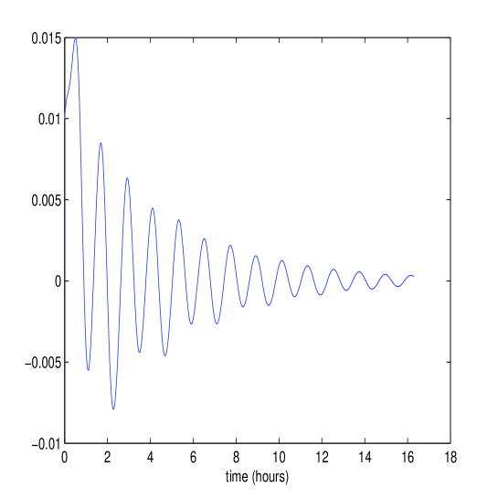
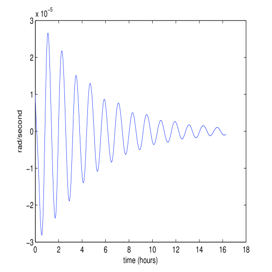
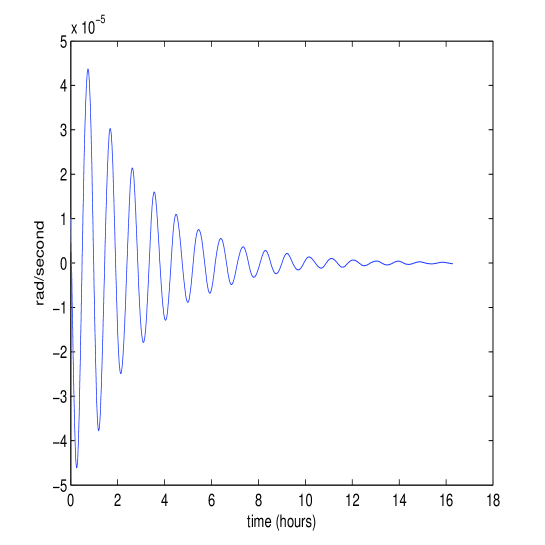
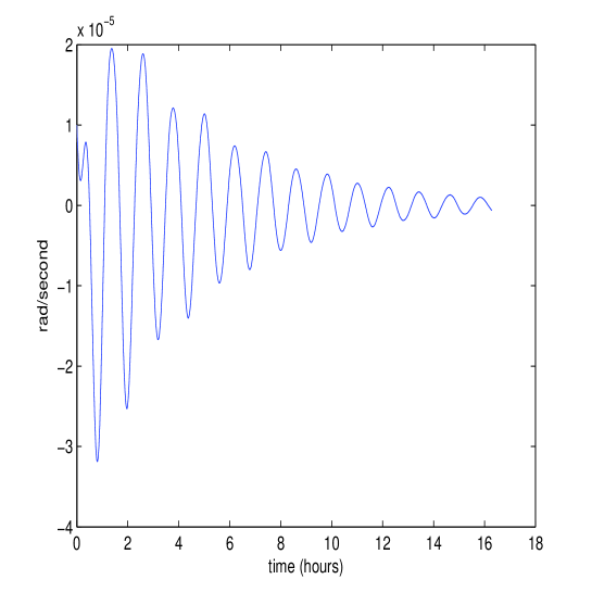
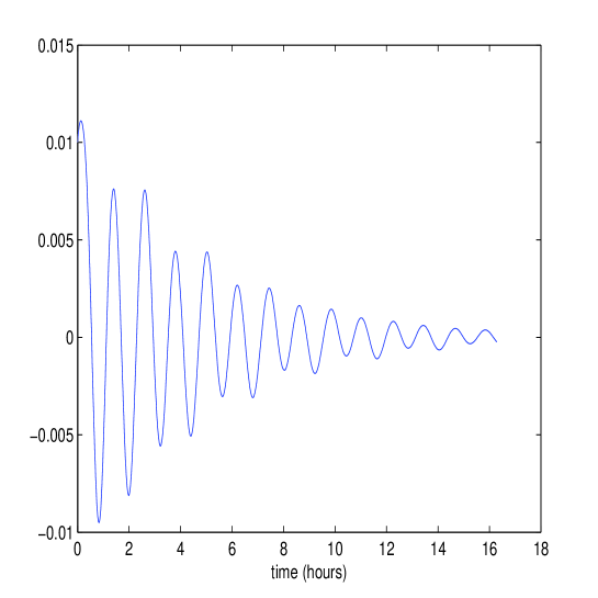
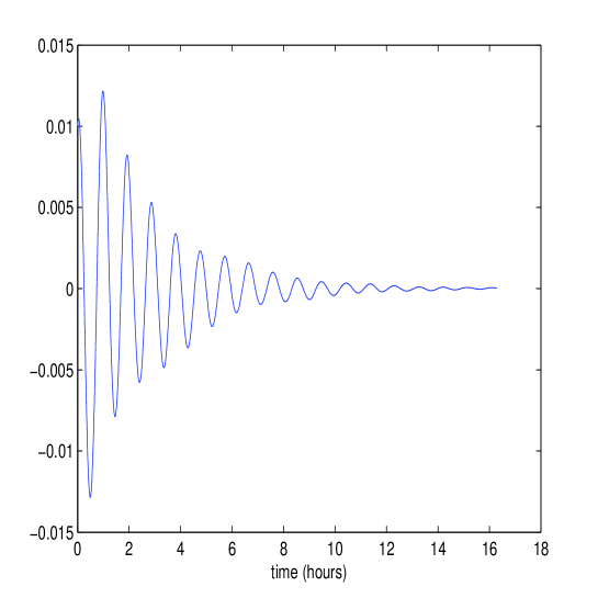
The orbital inclination $i_{m}=57C^{o}$, the orbit is circular with the altitude $657$ km. In view of equation (5), the orbital period is $5863$ seconds, and the orbital rate is $\omega_{0}=0.0011$ rad/second. Assuming that the total number of samples taken in one orbit is $100$, then, each sample period is $58.6352$ second. Select ${\bf Q}={\rm diag}(1.5*10^{-9},1.5*10^{-9},1.5*10^{-9},0.001,0.001,0.001)$ and ${\bf R}={\rm diag}(2*10^{-3},2*10^{-3},2*10^{-3})$. We have calculated and stored ${\bf P}_{k}$ for $k=0,1,2,\ldots,99$ using Algorithm 3.1. Assuming that the initial quaternion error is $(0.01,0.01,0.01)$ and the initial body rate is $(0.00001,0.00001,0.00001)$ radians per second, applying the feedback (66) to the system (59), the simulated spacecraft attitude response is given in Figures 1-6.

Figure 1: Attitude response $q_{1}$.

Figure 2: Attitude response $q_{2}$.

Figure 3: Attitude response $q_{3}$.

Figure 4: Body rate response $\omega_{1}$.

Figure 5: Body rate response $\omega_{2}$.

Figure 6: Body rate response $\omega_{3}$.

The designed controller stabilizes the spacecraft using only magnetic torques. This shows the effectiveness of the design method. Since this time-varying system has a long period $5863$ seconds and the number of samples in each period is $100$, this means that using $\boldsymbol{\Gamma}_{k}$ in (95) instead of $\boldsymbol{\Pi}_{k}$ in (90) saves about $100$ matrix inverses, a significant saving in the computation comparing to the well-known algorithm [26]!

5 Conclusion

In this paper, we proposed a new algorithm for the design of the periodic controller for the spacecraft using only magnetic torques. The proposed method is more efficient than existing methods because it makes full use of the information associated with this particular time-varying system. A simulation example is provided to demonstrate the effectiveness and fficiency of the algorithm. Although the algorithm is motivated by the problem of spacecraft attitude control using only magnetic torques, it can be used in any time-verying system $({\bf A},{\bf B}(t))$ where only ${\bf B}(t)$ is a periodically time-varying matrix.

References

• [1] Musser, K.L., and Ebert, W.L., โ€œAutonomous spacecraft attitude control using magnetic torquing only,โ€ Proceedings of the Flight Mechanics and Estimation Theory Symposium, NASA Goddard Apce Flight Center, Greenbelt, MD, pp. 23-38, 1989.
• [2] Pittelkau, M.E., โ€œOptimal periodic control for spacecraft pointing and attitude determination,โ€ Journal of Guidance, Control, and Dynamics, Vol. 16, No. 6, 1993, pp. 1078-1064.
• [3] Wisniewski, R., โ€œLinear time varying approach to satellite attitude control using only electromagnetic actuation,โ€ Proceedings of the AIAA Guidance, Navigation, and Control Conference, New Orleans, 1997, pp. 243-251.
• [4] Paiaki, M.L., โ€œMagnetic torque attitude control via asymptotic period linear quadratic requlation,โ€ Journal of Guidance, Control, and Dynamics, Vol. 24, No. 2, 2001, pp386-394.
• [5] Lovera, M., and Astolfi, A., โ€œSpacecraft attitude control using magnetic actuators,โ€ Automatica, Vol. 40, 2004, pp. 1405-1414.
• [6] Silani, E., and Lovera, M., โ€œMagnetic spacecraft attitude control: a survey and some new results,โ€ Control Engineering Practice, Vol. 13, 2005, pp. 357-371.
• [7] Lovera, M., and Astolfi, A., โ€œGlobal magnetic attitude control of spacecraft in the presence of gravity gradient,โ€ IEEE Transactions on Aerospace and Electronic System, Vol. 42, No.3, 2006, pp.796-805.
• [8] Yan, H., Ross, I.M., and Alfriend, K.T., โ€œPseudospectral feedback control for three-axes magnetic attitude stabilization in elliptic orbits,โ€ Journal of Guidance, Control, and Dynamics, Vol. 30, No. 4, 2007, pp. 1107-1115.
• [9] Pulecchi, T., Lovera, M., and Varga, A., โ€œOptimal discrete-time design of three-axis magnetic attitude control laws,โ€IEEE Transactions on Control System Technology, Vol. 18, No. 3, 2010, pp. 714-722.
• [10] Chen X., and Wu, X., โ€œModel predictive control of cube satellite with magnet-torque,โ€ Proceedings of the 2010 IEEE International Conference on Information and Automation, Harbin, China, 2010, pp. 997-1002.
• [11] Rehanoglu M., and Hervas, J.R., โ€œThree-axis magnetic attitude control algorithm for small satellites,โ€ Proceeding of the 5th International Conference on Recent Advance Technologies, Istanbul, 2011, pp. 897-902.
• [12] Zanchettin, A.M., and Lovera, M., โ€œHโˆžsubscript๐ปH_{\infty} attitude control of magnetically actuated satellite,โ€ Proceedings of 18th IFAC World Congress, Milano, Italy, 2011, pp. 8479-8484.
• [13] Bhat, S.P., โ€œControllability of nonlinear time-varying systems: application to spacecraft attitude control using magnetic actuation,โ€ IEEE Transactions on Automatic Control, Vol. 50, No. 11, 2005, pp. 1725-1735.
• [14] Yang, Y., โ€œControllability of spacecraft using only magnetic torques,โ€ to appear in IEEE Transactions on Aerospace and Electronic System, available in arXiv:1507.06963, 2015.
• [15] Yang, Y., โ€œQuaternion based model for momentum biased nadir pointing spacecraft,โ€ Aerospace Science and Technology, Vol. 14, No. 3, 2010, 199-202.
• [16] Yang, Y., โ€œAnalytic LQR design for spacecraft control system based on quaternion model,โ€ Journal of Aerospace Engineering, Vol. 25, No. 3, 2012, pp. 448-453.
• [17] Yang, Y., โ€œQuaternion based LQR spacecraft control design is a robust pole assignment design,โ€ Journal of Aerospace Engineering, Vol. 27, No. 1, 2014, , pp. 168-176.
• [18] Sidi, M.J., Spacecraft Dynamics and Control: A Practical Engineering Approach, Cambridge University Press, Cambridge, UK, 1997.
• [19] Wertz, J., Spacecraft Attitude Determination and Control, Kluwer Academic Publishers, Dordrecht, Holland, 1978.
• [20] Lewis, F.L., Vrabie, D., and Syrmos, V.L., Optimal Control, 3rd Edition, John Wiley & Sons, Inc., New York, USA, 2012.
• [21] Bittanti, S., โ€œPeriodic Riccati equation,โ€ The Riccati Equation, edited by S. Bittanti, et. al, Spriner, Berlin, 1991, pp. 127-162.
• [22] Laub, A.J., โ€œA Schur method for solving algebraic Riccati equations,โ€ IEEE Transactions on Automatic Control, Vol. 24, No. 6, 1979, pp. 913-921.
• [23] Vaughan D.R. โ€œA nonrecursive algebraic solution for the discrete Riccati equation,โ€ IEEE Transactions on Automatic Control, Vol. 15, No. 5, 1970, pp.597-599.
• [24] Laub, A.J., โ€œCanonical forms for ฯƒ๐œŽ\sigma-symplectic matrices,โ€ M.S. thesis, School of Mathematics, Univ. of Minnesota, MN, 1972.
• [25] Murnaghan, F.D., and Wintner, A., โ€œA canonical form for real matrices under orthogonal transformations,โ€ Proc. Nat. Acad. Sci., Vol. 17, 1931, pp. 417-420.
• [26] Hench, J.J., and Laub, A.J., โ€œNumerical solution of the discrete-time periodic Riccati equationโ€, IEEE Transactions on Automatic Control, Vol. 39, No.6, 1994, pp. 1197-1210.
• [27] Pappas, T., Laub, A.J., and Sandell, N.R., โ€œOn the numerical solution of the discrete-time algebraic Riccati equation,โ€ IEEE Transactions on Automatic Control, Vol. 25, No.4, 1980, pp. 631-641.