Bayesian Crossover Designs for Generalized Linear Models

 

Abstract

This article discusses optimal Bayesian crossover designs for generalized linear models. Crossover trials with $t$ treatments and $p$ periods, for $t<=p$, are considered. The designs proposed in this paper minimize the log determinant of the variance of the estimated treatment effects over all possible allocation of the $n$ subjects to the treatment sequences. It is assumed that the $p$ observations from each subject are mutually correlated while the observations from different subjects are uncorrelated. Since main interest is in estimating the treatment effects, the subject effect is assumed to be nuisance, and generalized estimating equations are used to estimate the marginal means. To address the issue of parameter dependence a Bayesian approach is employed. Prior distributions are assumed on the model parameters which are then incorporated into the $D_{A}$-optimal design criterion by integrating it over the prior distribution. Three case studies, one with binary outcomes in a $4\times 4$ crossover trial, second one based on count data for a $2\times 2$ trial and a third one with Gamma responses in a $3\times 2$ crossover trial are used to illustrate the proposed method. The effect of the choice of prior distributions on the designs is also studied. A general equivalence theorem is stated to verify the optimality of designs obtained.

Keywords: Bayesian designs; Count data; Efficiency; Gamma response; Generalized estimating equations; Logistic regression.  

1 Introduction

In this article we introduce Bayesian optimal crossover designs for generalized linear models (GLMs). Crossover trials with $t$ treatments and $p$ periods, for $t\leq p$ are considered. The designs selected minimize the log determinant of the variance-covariance matrix of the treatment effects, over all possible allocation of the $n$ subjects to the treatment sequences. Due to the dependence of the variance matrix on the model parameters a Bayesian approach is proposed.

Crossover designs were originally developed to be used in agricultural sciences (Cochran (1939)). Later, these repeated measurement designs were found to be useful in many other fields, such as pharmaceutical and clinical trials, bioequivalence and biological studies. Optimal crossover designs for normal response have been studied by many reserachers, namely Hedayat and Afsarinejad (1975, 1978), Cheng and Wu (1980), Laska et al. (1983), Laska and Meisner (1985), Stufken (1991), Carrire and Reinsel (1993), Kushner (1997, 1998) and Carriere and Huang (2000). For a detailed review of crossover designs, we would like to refer to the paper by Bose and Dey (2013) and books by Bose and Dey (2009), Senn (2002) and Jones and Kenward (2014).

Most of the available literature on optimal crossover designs (as discussed above) mainly focuses on normal responses. However, in biological studies, very often we find responses that are non-normal (Layard and Arvesen (1978) and Forster (1992)) and have to be modeled using a generalized linear model (GLM). While methods for analyzing GLM data arising from crossover trials are available in Senn (2002) and Jones and Kenward (2014), the question of designing such studies for GLMs in an optimal manner does not seem to have been much explored in the statistical literature. Waterhouse et al. (2006) studied optimal $2\times 2$ crossover trial for binary data in some special cases, like the carryover effect is proportional to the direct treatment effect and no period effects are considered. Adaptive crossover designs restricted to two period two treatment binary data useful in clinical trials have also been investigated by Bandyopadhyay et al. (2009).

In this article, we study optimal Bayesian crossover designs for GLMs. Three case studies based on non-normal responses are used to illustrate the proposed methodology. Generalized estimating equations of Liang and Zeger (1986) are used to estimate the marginal means. The correlation between observations within subjects are modeled using a “working correlation structure”, which is assumed to be compound symmetric or auto regressive in nature. Since the main interest is in estimating the treatment effects, the subject effects as taken as nuisance parameters. As in all GLM designs, the variance of the treatment effect estimator depends on the model parameters. To address the issue of the parameter dependence and obtain robust designs we propose the Bayesian approach to design selection. Bayesian designs have been a popular choice whenever the variance-covariance matrix depends on the model parameters, for some references see (Chaloner and Larntz (1989), Dette and Sperlich (1994), Woods and Van de Ven (2011) and Mylona et al. (2014) ). In our approach, a prior distribution is assumed on the model parameters, which is then incorporated into an appropriate objective function (variance of the treatment contrast) by integrating and averaging over the prior distribution. Similar to our Bayesian design criterion, an average criterion called $A$-criterion have been used before for crossover designs for normal responses by (Kempton et al. (2001), Baily and Kunert (2006), Zheng (2013) and Li et al. (2015)).

2 Case studies

For illustration purpose we consider three case studies based on crossover trials involving binary, count and Gamma responses.

2.1 A four periods four treatments binary response crossover trial

The first case study presented here is from a trial based on the four-period, four treatment Williams design. It has been reported in Kenward and Jones (1992). The four treatments are denoted by $A,B,C$ and $D$. Eighty subjects are randomly assigned to the four treatment sequences {$ABCD,BDAC,CADB,DCBA$}, with about twenty subjects allocated to each treatment sequence. The response is a binary outcome taking values 1 and 0 based on patient relief and no relief, respectively.

The research question which arises from the above case study is why did the experimenter select the 4 treatment sequences {$ABCD,BDAC,CADB,DCBA$} forming a Williams design (Williams (1949)). Is this the best possible selection of treatment sequences? The book by Bose and Dey (2009), page 40 shows that for normal response crossover models, for the 4 treatment and 4 periods case, Williams design is the optimal design. But can we be sure that the same design applies to a binary response crossover framework as well? Does the selected design change if the correlation structure between observations change say, from equicorrelated to auto regressive structure?

2.2 Two periods two treatments Poisson response crossover trial

This study is based on an example described in Layard and Arvesen (1978). Two drugs, standard drug A and an innovation drug B, is administered for controlling angina in 20 patients. It is known that the innovative drug $B$ is no worse than the standard drug $A$. For a given patient, number of angina attacks on weekly basis is assumed to follow a Poisson distribution (Layard and Arvesen (1978)). Number of attacks for each patient of consecutive two weeks are recorded. Treatment sequences considered are {$AB$, $BA$} and 10 patients are assigned to each of the treatment sequences. This is a 2-treatments 2-periods crossover trial.

As in case study I, the question arises why does the experimenter choose the design $\{AB,BA$}. Is this the best or most efficient design under the repeated measures setup when responses follow a Poisson distribution?

2.3 Three periods two treatments Gamma response trial

The length of hospital stay is an important measure of the success of hospital activity, costs incurred by patients and the treatment administered to a patient. However, its empirical distribution is often right skewed and a Gamma distribution with a log link has been seen to be a good fit (Faddy et al. (2009)). In this case study we consider a crossover trial where two treatments are applied over three periods and length of hospital stay, assumed to having a Gamma distribution, is the primary end point.

As in the earlier two case studies, we investigate the best design for a two treatment three periods design with a gamma response.

3 The model

We consider experiments where there are $t$ treatments and $n$ subjects, and $p$ repeated measurements are taken from each subject. The observations from each subject may be correlated. The marginal distribution of the response $Y_{ij}$ is described by a working generalized linear model with the following three components (Liang and Zeger (1986)):

1. $Y_{ij}$ has a distribution from the exponential family form,

   $$f(y_{ij}|\phi_{ij},\psi)=\mbox{exp}\left\{\left[y_{ij}\phi_{ij}-b(\phi_{ij})+c(y_{ij})\right]\psi+d(y_{ij},\psi)\right\}$$ (1)

   where $\phi_{ij}$ is a function of the model parameters, $b(\cdot)$, $c(\cdot)$ and $d(\cdot)$ are known functions and $\psi$ is the dispersion parameter. It can be shown that: ${E}(Y_{ij})=\mu_{ij}=\frac{db(\phi_{ij})}{d\phi_{ij}}$ and ${Var}(Y_{ij})=\frac{d^{2}b(\phi_{ij})}{d\phi^{2}_{ij}}/\psi$.

2. The linear predictor $\eta_{ij}$ in a repeated measures setup can be written as (Bose and Dey (2009)),

   $$\eta_{ij}=\nu+\beta_{i}+\tau_{d(i,j)}+\gamma_{d(i-1,j)};\,i=1\,\ldots,p,\,j=1,\ldots,n,$$ (2)

   where $\nu$ is the fixed unknown parameter, $\beta_{i}$ represents the effect of the $i$th period, $\tau_{s}$ is the direct effect due to treatment $s$ and $\gamma_{s}$ is the carryover effect due to treatment $s$, $s=1,\ldots,t$. It is assumed that $\gamma_{d(0,j)}=0$.

3. The mean of $y_{ij}$ denoted by $\mu_{ij}$ is related to $\eta_{ij}$ through a link function $g$, where $g(\mu_{ij})=\eta_{ij}$ and the inverse of $g$ exists.

3.1 Estimation

Regression coefficients as well as their variances are estimated by the GEE approach of Liang and Zeger (1986) and Zeger et al. (1988). Due to observations from the same subject being correlated, a “working correlation” matrix, $R(\alpha)$, is used to describe the dependencies between repeated observations from a subject. Here $\alpha$ is a vector of length $l$, which fully characterizes $R(\alpha)$ (Liang and Zeger (1986)). For cases where $R(\alpha)$ is the true correlation matrix of $\mathbf{Y}_{j}=(Y_{1j},\cdots,Y_{pj})^{\prime}$, the covariance of $\mathbf{Y}_{j}$ is

$$V_{j}=A_{j}^{1/2}R(\alpha)A_{j}^{1/2},$$ (3)

$A_{j}=\text{diag}(\text{Var}(Y_{1j}),\ldots,\text{Var}(Y_{pj}))$. If the correlation structure is compound symmetric that is corr($Y_{ij},Y_{i^{\prime}j}$) = $\alpha$ for all $i\neq i^{\prime}$, then $l=1$, if the correlation structure is left unspecified then $l=\frac{p(p-1)}{2}$. Also, the asymptotic variance for the GEE estimator $\hat{\boldsymbol{\theta}}$ (see Zeger et al. (1988), equation (3.2)) is

$$Var(\hat{\boldsymbol{\theta}})=\left[\sum_{j=1}^{n}\frac{\partial\mu^{\prime}_{j}}{\partial\boldsymbol{\theta}}V_{j}^{-1}\frac{\partial\mu_{j}}{\partial\boldsymbol{\theta}}\right]^{-1},$$ (4)

where $\boldsymbol{\theta}=(\nu,\boldsymbol{\beta}^{\prime},\boldsymbol{\tau}^{\prime},\boldsymbol{\gamma}^{\prime})^{\prime}$, $\boldsymbol{\beta}^{\prime}=(\beta_{1},\cdots\beta_{p})$, $\boldsymbol{\tau}^{\prime}=(\tau_{1},\cdots,\tau_{t})$ and $\boldsymbol{\gamma}^{\prime}=(\gamma_{1},\cdots,\gamma_{t})$.

However, if the true correlation structure varies from the “working correlation” structure, then $Var(\hat{\boldsymbol{\theta}})$ is given by the sandwich formula (Zeger et al. (1988), equation (3.2))

$$Var(\hat{\boldsymbol{\theta}})=\left[\sum_{j=1}^{n}\frac{\partial\mu^{\prime}_{j}}{\partial\boldsymbol{\theta}}V_{j}^{-1}\frac{\partial\mu_{j}}{\partial\boldsymbol{\theta}}\right]^{-1}\left[\sum_{j=1}^{n}\frac{\partial\mu^{\prime}_{j}}{\partial\boldsymbol{\theta}}V_{j}^{-1}Cov(Y_{j})V_{j}^{-1}\frac{\partial\mu_{j}}{\partial\boldsymbol{\theta}}\right]\left[\sum_{j=1}^{n}\frac{\partial\mu^{\prime}_{j}}{\partial\boldsymbol{\theta}}V_{j}^{-1}\frac{\partial\mu_{j}}{\partial\boldsymbol{\theta}}\right]^{-1}.$$ (5)

For the crossover model (1), the $i$th element of $\frac{\partial\mu_{j}}{\partial\boldsymbol{\theta}}$ is $\frac{\partial\mu_{ij}}{\partial\boldsymbol{\theta}}=x^{\prime}_{ij}\frac{\partial g^{-1}(\eta_{ij})}{\partial\eta_{ij}}$, where $x^{\prime}_{ij}$ is the $i$th row of $X_{j}$ for $i=1,\ldots,p$. The design matrix is $X_{j}=[1_{p}\;P_{j}\;T_{j}\;F_{j}]$, where $P_{j}=I_{p}$; $T=(T^{\prime}_{1},\ldots,T^{\prime}_{n})^{\prime}$, where $T_{j}$ is a $p\times t$ matrix with its $(i,s)$th entry equal to 1 if subject $j$ receives the direct effect of the treatment $s$ in the $i$th period and zero otherwise; $F=(F^{\prime}_{1},\ldots,F^{\prime}_{n})^{\prime}$, where $F_{j}$ is a $p\times t$ matrix with its $(i,s)$th entry equal to 1 if subject $j$ receives the carryover effect of the treatment $s$ in the $i$th period and zero otherwise.

3.2 Specific case: Bernoulli distribution

If $Y_{ij}\sim\mbox{Bernoulli}(\mu_{ij})$, then the probability mass function of $Y_{ij}$ is:

$$f(y_{ij}|\mu_{ij})=\mbox{exp}\left\{y_{ij}\mbox{log}\frac{\mu_{ij}}{1-\mu_{ij}}+\mbox{log}(1-\mu_{ij})\right\}$$

Comparing with equation (1), we get $\phi_{ij}=\mbox{log}\frac{\mu_{ij}}{1-\mu_{ij}}$, $b(\phi_{ij})=-\mbox{log}(1-\mu_{ij})=\mbox{log}(1+\mbox{exp}(\phi_{ij}))$, $c(y_{ij})=0$, $\psi=1$ and $d(y_{ij},\psi)=0$. The mean of $Y_{ij}$ is $\mbox{E}(Y_{ij})=\mu_{ij}=\frac{db(\phi_{ij})}{d\phi_{ij}}=\frac{\mbox{exp}(\phi_{ij})}{1+\mbox{exp}(\phi_{ij})}$, and $\mbox{Var}(Y_{ij})=\frac{d^{2}b(\phi_{ij})}{d\phi^{2}_{ij}}/\psi=\frac{\mbox{exp}(\phi_{ij})}{(1+\mbox{exp}(\phi_{ij}))^{2}}=\mu_{ij}(1-\mu_{ij})$.

Considering the logit link function to relate the linear predictor $\eta_{ij}$ to the mean $\mu_{ij}$, $g(\mu_{ij})=\mbox{log}\frac{\mu_{ij}}{1-\mu_{ij}}$. Thus $g^{-1}(\eta_{ij})=\frac{\mbox{e}^{\eta_{ij}}}{1+\mbox{e}^{\eta_{ij}}}$, and the $i$th component of $\frac{\partial\mu_{j}}{\partial\boldsymbol{\theta}}$ is $\frac{\partial\mu_{ij}}{\partial\boldsymbol{\theta}}=x^{\prime}_{ij}\frac{\partial g^{-1}(\eta_{ij})}{\partial\eta_{ij}}=x^{\prime}_{ij}\frac{\mbox{e}^{\eta_{ij}}}{(1+\mbox{e}^{\eta_{ij}})^{2}}=x^{\prime}_{ij}\mu_{ij}(1-\mu_{ij})$. This implies $\frac{\partial\mu_{j}}{\partial\boldsymbol{\theta}}=D_{j}X_{j}$, where $D_{j}$ is the diagonal $p\times p$ matrix with elements $\mu_{ij}(1-\mu_{ij}),i=1,\cdots,p$. The matrix $A_{j}$ defined in equation (3) is same as $D_{j}$ in this case. Using equation (4), the asymptotic information matrix is:

$$\sum_{j=1}^{n}\frac{\partial\mu^{\prime}_{j}}{\partial\boldsymbol{\theta}}V_{j}^{-1}\frac{\partial\mu_{j}}{\partial\boldsymbol{\theta}} = \sum_{j=1}^{n}X^{\prime}_{j}D_{j}A_{j}^{-1/2}R^{-1}(\alpha)A_{j}^{-1/2}D_{j}X_{j}$$

$$= \sum_{j=1}^{n}X^{\prime}_{j}A_{j}^{1/2}R^{-1}(\alpha)A_{j}^{1/2}X_{j}.$$

3.3 Specific case: Poisson distribution

If $Y_{ij}\sim\mbox{Poisson}(\mu_{ij})$, then the probability mass function of $Y_{ij}$ is:

$$f(y_{ij}|\mu_{ij})=\mbox{exp}\left\{y_{ij}\mbox{log}(\mu_{ij})-\mu_{ij}-\mbox{log}(y_{ij}!)\right\}$$

Comparing with equation (1), we get $\phi_{ij}=\mbox{log}(\mu_{ij})$, $b(\phi_{ij})=\mu_{ij}=\mbox{e}^{\phi_{ij}}$, $c(y_{ij})=-\mbox{log}(y_{ij}!)$, $\psi=1$ and $d(y_{ij},\psi)=0$. The mean of $Y_{ij}$ is $\mbox{E}(Y_{ij})$ = $\mu_{ij}=\mbox{e}^{\phi_{ij}}$ and $\mbox{Var}(Y_{ij})=\mbox{e}^{\phi_{ij}}=\mu_{ij}$.

Using the log link we obtain, $g(\mu_{ij})=\mbox{log}(\mu_{ij})=\eta_{ij}$, and the $i$th component of $\frac{\partial\mu_{j}}{\partial\boldsymbol{\theta}}$ is $\frac{\partial\mu_{ij}}{\partial\boldsymbol{\theta}}=x^{\prime}_{ij}\frac{\partial g^{-1}(\eta_{ij})}{\partial\eta_{ij}}=x^{\prime}_{ij}\mbox{e}^{\eta_{ij}}=x^{\prime}_{ij}\mu_{ij}$. This implies $\frac{\partial\mu_{j}}{\partial\boldsymbol{\theta}}=D_{j}X_{j}$, where $D_{j}$ is the diagonal $p\times p$ matrix with elements $\mu_{ij},i=1,\cdots,p$. The matrix $A_{j}$ defined in equation (3) is again same as $D_{j}$ in this case. The asymptotic information matrix is:

$$\sum_{j=1}^{n}\frac{\partial\mu^{\prime}_{j}}{\partial\theta}V_{j}^{-1}\frac{\partial\mu_{j}}{\partial\theta} = \sum_{j=1}^{n}X^{\prime}_{j}D_{j}A_{j}^{-1/2}R^{-1}(\alpha)A_{j}^{-1/2}D_{j}X_{j}$$

$$= \sum_{j=1}^{n}X^{\prime}_{j}A_{j}^{1/2}R^{-1}(\alpha)A_{j}^{1/2}X_{j}.$$

3.4 Specific case: Gamma distribution

If $Y_{ij}\sim\mbox{Gamma}(\kappa,\lambda_{ij})$, where $\kappa>0$ is the shape parameter and $\lambda_{ij}>0$ is the rate parameter. Then the probability density function of $Y_{ij}$ is:

$$f(y_{ij}|\lambda_{ij},\kappa)=\mbox{exp}\left\{\left[y_{ij}\left(-\frac{\lambda_{ij}}{\kappa}\right)+\mbox{log}\left(\frac{\lambda_{ij}}{\kappa}\right)+\mbox{log}(y_{ij})\right]{\kappa}+\kappa\mbox{log}(\kappa)-\mbox{log}(y_{ij})-\mbox{log}\Gamma\kappa\right\}$$

Comparing with equation (1), we get $\phi_{ij}=-\frac{\lambda_{ij}}{\kappa}$, $b(\phi_{ij})=-\mbox{log}(\frac{\lambda_{ij}}{\kappa})=-\mbox{log}(-\phi_{ij})$, $c(y_{ij})=\mbox{log}(y_{ij})$, $\psi=\kappa$ and $d(y_{ij},\psi)=\kappa\mbox{log}(\kappa)-\mbox{log}{(y_{ij})}({\Gamma\kappa})=\psi\mbox{log}(\psi)-\mbox{log}{(y_{ij})}({\Gamma\psi})$. The mean of $Y_{ij}$ is $\mbox{E}(Y_{ij})=\mu_{ij}=\kappa/\lambda_{ij}$ and $\mbox{Var}(Y_{ij})=\frac{k}{\lambda_{ij}^{2}}=\frac{\mu_{ij}^{2}}{\kappa}$.

In case of a log link function, $g(\mu_{ij})=\mbox{log}(\mu_{ij})=\eta_{ij}$. The $i$th component of $\frac{\partial\mu_{j}}{\partial\boldsymbol{\theta}}$ is $\frac{\partial\mu_{ij}}{\partial\boldsymbol{\theta}}=x^{\prime}_{ij}\frac{\partial g^{-1}(\eta_{ij})}{\partial\eta_{ij}}=x^{\prime}_{ij}\mbox{e}^{\eta_{ij}}=x^{\prime}_{ij}\mu_{ij}$. This implies $\frac{\partial\mu_{j}}{\partial\boldsymbol{\theta}}=D_{j}X_{j}$, where $D_{j}$ is the diagonal $p\times p$ matrix with elements $\mu_{ij},i=1,\cdots,p$. The matrix $A_{j}$ defined in equation (3) is diagonal $p\times p$ matrix with elements $\frac{\mu_{ij}^{2}}{\kappa},i=1,\cdots,p$. The asymptotic information matrix is:

$$\sum_{j=1}^{n}\frac{\partial\mu^{\prime}_{j}}{\partial\theta}V_{j}^{-1}\frac{\partial\mu_{j}}{\partial\theta} = \sum_{j=1}^{n}X^{\prime}_{j}D_{j}A_{j}^{-1/2}R^{-1}(\alpha)A_{j}^{-1/2}D_{j}X_{j}$$

$$= \sum_{j=1}^{n}X^{\prime}_{j}\left\{\sqrt{\kappa}I_{p}\right\}R^{-1}(\alpha)\left\{\sqrt{\kappa}I_{p}\right\}X_{j}$$

$$= \kappa\sum_{j=1}^{n}X^{\prime}_{j}R^{-1}(\alpha)X_{j}.$$

In case of a reciprocal link function, $g(\mu_{ij})=\frac{1}{\eta_{ij}}$. The $i$th component of $\frac{\partial\mu_{j}}{\partial\boldsymbol{\theta}}$ is $\frac{\partial\mu_{ij}}{\partial\boldsymbol{\theta}}=x^{\prime}_{ij}\frac{\partial g^{-1}(\eta_{ij})}{\partial\eta_{ij}}=-\frac{x^{\prime}_{ij}}{{\eta_{ij}^{2}}}=-x^{\prime}_{ij}\mu_{ij}^{2}$. This implies $\frac{\partial\mu_{j}}{\partial\boldsymbol{\theta}}=D_{j}X_{j}$, where $D_{j}$ is the diagonal $p\times p$ matrix with elements $-\mu_{ij}^{2},i=1,\cdots,p$. The matrix $A_{j}$ defined in equation (3) is A diagonal $p\times p$ matrix with elements $\frac{\mu_{ij}^{2}}{\kappa},i=1,\cdots,p$. The asymptotic information matrix can be written as:

$$\sum_{j=1}^{n}\frac{\partial\mu^{\prime}_{j}}{\partial\theta}V_{j}^{-1}\frac{\partial\mu_{j}}{\partial\theta} = \sum_{j=1}^{n}X^{\prime}_{j}D_{j}A_{j}^{-1/2}R^{-1}(\alpha)A_{j}^{-1/2}D_{j}X_{j}$$

$$= \sum_{j=1}^{n}X^{\prime}_{j}\left\{-\sqrt{\kappa}D_{j}^{*}\right\}R^{-1}(\alpha)\left\{-\sqrt{\kappa}D_{j}^{*}\right\}X_{j}$$

$$= \kappa\sum_{j=1}^{n}X^{\prime}_{j}D_{j}^{*}R^{-1}(\alpha)D_{j}^{*}X_{j},$$

where $D_{j}^{*}$ is the diagonal matrix with diagonal elements $\mu_{ij},i=1,\cdots,p$.

Note that the shape parameter $\kappa$ is a multiplicative constant in the expression of the information matrices and hence does not affect design selection.

4 Approximate designs

For finding optimal crossover designs for the logistic model we use the approximate theory as in Laska et al. (1983) and Kushner (1997, 1998). Suppose ${\Omega}$ is the set of treatment sequences of the form $\omega=(t_{1},\ldots,t_{p})^{\prime},\,t_{i}\in\{1,\ldots,t\}$, and $n_{\omega}$ is the number of subjects assigned to sequence $\omega$. Then, $n=\sum_{\omega\in\Omega}n_{\omega},n_{\omega}\geq 0$. A design $\zeta$ in approximate theory is specified by the set $\{p_{\omega},\omega\in\Omega\}$ where $p_{\omega}=n_{\omega}/n$, is the proportion of subjects assigned to treatment sequence $\omega$.

The matrices $T_{j}$ and $F_{j}$ depend only on the treatment sequence $\omega$ to which the $j$th subject is assigned, so $T_{j}=T_{\omega},\,F_{j}=F_{\omega}$, implying, $X_{j}=X_{\omega}$. Thus, the variance of $\hat{\boldsymbol{\theta}}$ is

$$Var_{\zeta}(\hat{\boldsymbol{\theta}})=\left[\sum_{\omega\in\Omega}np_{\omega}\frac{\partial\mu^{\prime}_{\omega}}{\partial\boldsymbol{\theta}}V_{\omega}^{-1}\frac{\partial\mu_{\omega}}{\partial\boldsymbol{\theta}}\right]^{-1}\left[\sum_{\omega\in\Omega}np_{\omega}\frac{\partial\mu^{\prime}_{\omega}}{\partial\boldsymbol{\theta}}V_{\omega}^{-1}Cov(Y_{\omega})V_{\omega}^{-1}\frac{\partial\mu_{\omega}}{\partial\boldsymbol{\theta}}\right]\left[\sum_{\omega\in\Omega}np_{\omega}\frac{\partial\mu^{\prime}_{\omega}}{\partial\boldsymbol{\theta}}V_{\omega}^{-1}\frac{\partial\mu_{\omega}}{\partial\boldsymbol{\theta}}\right]^{-1}.$$ (6)

If the true correlation of $Y_{j}$ is equal to $R(\alpha)$ then we have a much simpler form,

$$Var_{\zeta}(\hat{\boldsymbol{\theta}})=\left[\sum_{\omega\in\Omega}np_{\omega}\frac{\partial\mu^{\prime}_{\omega}}{\partial\boldsymbol{\theta}}V_{\omega}^{-1}\frac{\partial\mu_{\omega}}{\partial\boldsymbol{\theta}}\right]^{-1}.$$ (7)

4.1 Design criterion

In repeated measures trials when the interest is in only estimating direct treatment effect contrasts, we may instead work with $Var(\hat{\boldsymbol{\tau}})$ given by,

$$Var_{\zeta}(\hat{\boldsymbol{\tau}})=EVar_{\zeta}(\hat{\boldsymbol{\theta}})E^{\prime},$$ (8)

where $E$ is a $t\times m$ matrix given by $[0_{t1},0_{tp},I_{t},0_{tt}]$ and $m$ is the total number of parameters in $\boldsymbol{\theta}$. Here by $0_{p_{1}p_{2}}$ we mean a $p_{1}\times p_{2}$ matrix of zeros.

The design minimizing the criterion

$$\Lambda(\zeta,\boldsymbol{\theta},\alpha)=\log\text{Det}(Var_{\zeta}(\hat{\boldsymbol{\tau}})).$$ (9)

is known as the $D_{A}$-optimal design (Atkinson et al. (2007) , page 137). Since it is a GLM the variance depends on the model parameters as well as the covariance parameters, and the design obtained is locally optimal.

To obtain $D_{A}$-optimal designs robust to uncertainties in the parameters we propose a Bayesian approach. This method has been used before for logistic regression by Chaloner and Larntz (1989), and Dror and Steinberg (2006) and for block designs by Woods and Van de Ven (2011). For repeated measures models, the design which minimizes

$$\Psi(\mathfrak{B},\zeta,\alpha)=\int_{\mathfrak{B}}\Lambda(\zeta,\boldsymbol{\theta},\alpha)\,dF(\boldsymbol{\theta}),$$ (10)

where $\mathfrak{B}\subset\mathbb{R}^{m}$ is the parameter space of parameter vector $\boldsymbol{\theta}$ and $F(\boldsymbol{\theta})$ is a proper prior distribution for $\boldsymbol{\theta}$, is the $D_{A}$-optimal Bayesian crossover design (or the average $D_{A}$-optimal design of Pettersson (2005)). Note, for all working examples (in Sections 5.1, 5.2 and 5.3) no prior distributions are assigned to the correlation parameters $\alpha$, designs are obtained only for some fixed values chosen for $\alpha$. However, in Section 7 we investigated the design performance when there are priors on $\alpha$.

In our computations we have used both uniform and normal priors for $\boldsymbol{\theta}$. The minimization of the objective function in (10) with respect to $\zeta$, requires high-dimensional integral calculation. Similar to Woods and Van de Ven (2011), Latin Hypercube Sampling (LHS) has been used for deriving an approximate solution of the above optimization problem.

For evaluating the performance of design $\zeta$ with respect to the reference design $\zeta^{*}$ ($D_{A}$-optimal Bayesian design), we use an efficiency criterion defined as:

$$Eff_{D}(\zeta,\zeta^{*},\mathfrak{B},\alpha)=\left[\mbox{exp}\left\{\Psi(\mathfrak{B},\zeta^{*},\alpha)-\Psi(\mathfrak{B},\zeta,\alpha)\right\}\right]^{1/m},$$ (11)

here $m$ is the number of model parameters. Similar efficiency function has been used before by Woods et al. (2006).

Working correlation matrix structures such as the compound symmetric (or equi-correlated) and the AR(1) are investigated. Under the equi-correlated covariance structure, $R_{j}=(1-\alpha)I_{p}+\alpha J_{p}$, and under the AR(1) assumption, $R_{j}=\alpha^{|i-i^{\prime}|},\,i\neq i^{\prime}.$

5 Examples

5.1 Example 1: Four periods, four treatments binary response trial

In Case study 1, a four periods four treatments crossover trial described in Kenward and Jones (1992) is considered. There are eighty subjects allocated to the four treatment sequences, with about twenty subjects per sequence. Treatments are denoted by $A$, $B$, $C$ and $D$. The treatment sequences form a Williams design given as follows:

$$\begin{bmatrix}A&B&C&D\\ B&D&A&C\\ C&A&D&B\\ D&C&B&A\end{bmatrix}$$

The response variable is binary in nature. The data set is available in Table 3 of Kenward and Jones (1992). For a four periods, four treatments trial, there are 24 possible Latin square designs (LSDs) with every treatment represented once and only once in each row and in each column (see Table 5.1 Senn (2002)). A special form of Latin square design is called Williams square design (WSD) in which every treatment follows every other treatment only once. In the case of normal responses when $t=p$ and $t$ is even, for reduced models (no carryover effects) LSD and for full models (carryover effects present) WSDs are variance balanced designs (Lawson (2014), page 361). However, these designs may not be optimal in general. But under some subject constraints WSD is universally optimal for even $t$, $n\leq t(t+2)/2$ and $4\leq t\leq 12$ (Bose and Dey (2009), page 40).

Instead of using equation (2) directly as the linear predictor $\eta_{ij}$ we use a reparametrized version ,

$$\eta_{ij}=\nu+\beta_{1}^{*}P_{1}+\beta_{2}^{*}P_{2}+\beta_{3}^{*}P_{3}+\tau_{1}^{*}T_{1}+\tau_{2}^{*}T_{2}+\tau_{3}^{*}T_{3}+\gamma_{1}^{*}C_{1}+\gamma_{2}^{*}C_{2}+\gamma_{3}^{*}C_{3},$$ (12)

where

	$P_{1}$	$P_{2}$	$P_{3}$
Period 1	0	0	0
Period 2	1	0	0
Period 3	0	1	0
Period 4	0	0	1

$T_{i}$’s and $C_{i}$’s for $i=1,\cdots,4$, are similarly defined. Also, $\beta_{1}=0$, $\beta_{i}=\beta^{*}_{i-1},\,i=2,\ldots,4$, $\tau_{A}=0$, $\tau_{B}=\tau^{*}_{1}$, $\tau_{C}=\tau^{*}_{2}$, $\tau_{D}=\tau^{*}_{3}$ , $\gamma_{A}=0$, $\gamma_{B}=\gamma^{*}_{1}$, $\gamma_{C}=\gamma^{*}_{2}$ and $\gamma_{D}=\gamma^{*}_{3}$. Note that carryover effect in the first period is taken to be zero. It is noted that total number of parameters reduces to $m^{*}=m-3$, where $m$ in equation (2) was 13 for a $4\times 4$ design. The $E$ matrix defined in equation (8) will be of same form but $m$ is replaced by $m^{*}$.

Point estimates and corresponding confidence intervals of the parameters are calculated using PROC GENMOD procedure in SAS software (SAS Institute Inc. (2003)). Results are summarized in Table 1 for both reduced and full models. In a reduced model it is assumed that there are no carryover treatment effects, while in a full model both direct and carryover treatment effects are assumed to be present. The working correlation structure is taken to be compound symmetric (CS) in nature, the correlation coefficient is estimated to be 0.215.

Table 1: Point estimates and confidence intervals for both reduced and full models under the compound symmetric correlation structure (Example 1).

Parameter	Point estimate [95%Confidence interval]
	no carryover effect	with carryover effect
$\nu$	1.0980 [0.4232 1.7728]	1.0158 [0.3474  1.6842]
$\beta_{1}^{*}$	-0.3056 [-0.8643 0.2532]	-0.5525 [-1.2565  0.1515]
$\beta_{2}^{*}$	-0.2414 [-0.8228  0.3399]	-0.4842 [-1.2034  0.2349]
$\beta_{3}^{*}$	0.3817 [-0.2391  1.0026]	0.1234 [-0.6888  0.9356]
$\tau_{1}^{*}$	-0.3270 [-0.8660 0.2119]	-0.2564 [-0.8075  0.2948]
$\tau_{2}^{*}$	-0.0681 [-0.6996 0.5635]	0.0069 [-0.6473  0.6610]
$\tau_{3}^{*}$	-0.5322 [-1.1684 0.1041]	-0.3736 [-1.0165  0.2693]
$\gamma_{1}^{*}$	-	0.1786 [-0.5965  0.9538]
$\gamma_{2}^{*}$	-	0.2242 [-0.5443  0.9927]
$\gamma_{3}^{*}$	-	0.6620 [-0.1352 1.4591]

For a $4\times 4$ crossover trial the number of all possible treatment sequences are $4^{4}=256$. However, in this example we restrict our design space to only 16 treatment sequences, i.e., $\Omega=$ {$ACDB$, $BDCA$, $CBAD$, $DABC$, $ADCB$, $BCDA$, $CABD$, $DBAC$, $AABB$, $BBAA$, $CCDD$, $DDCC$, $AAAB$, $BBBA$, $CCCD$, $DDDC$}. These sequences are chosen since they can be used to form LSDs (including WSDs) and also non LSD crossover designs. Note in the normal response case it has been reported that WSDs under certain constraints are universally optimal for the 4 treatment and 4 period case. Thus, we felt it was enough to restrict $\Omega$ to these 16 sequences. Also lowering the number of treatment sequences increases our computational speed. The Bayesian designs found, also satisfy the conditions of the equivalence theorem given in the appendix.

The following prior distributions are considered for the model parameters, $\boldsymbol{\theta}$, for obtaining the Bayesian optimal design:

• Cartesian product of 95% confidence intervals of parameters given in Table 1.

• Cartesian product of the nonnegative part of 95% confidence intervals of parameters given in Table 1.

• and 4: Independent multivariate normal distribution with mean vector as the point estimates of the parameters given in Table 1 and (for prior 3) the variance is 0.25, (for prior 4) the variance is 0.50.

Note prior 2 is asymmetric around 0 and priors 3 and 4 are the normal priors with different variances. The Bayesian crossover design is obtained by minimizing formula 10, and denoting it by $D^{B}$.

The performance of $D^{B}$ is compared with 24 LSDs including 6 WSDs, and 24 extra period designs (EPDs) (a design in which first three rows correspond to a LSD and the last row is same as the previous one (Patterson and Lucas (1959)). We noted that the performance of each LSD is same among the 18 LSDs under the reduced and full models for both of the correlation structures and priors used. Same is true for 6 WSDs and 24 EPDs. Thus the results are based on one LSD, one WSD and one EPD.

5.1.1 Reduced model: No carryover effects

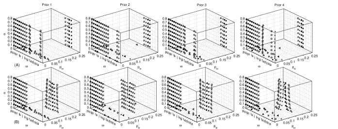
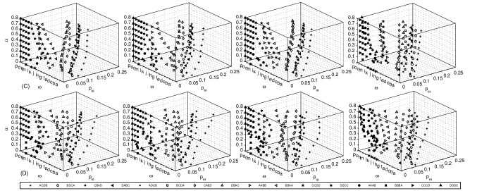
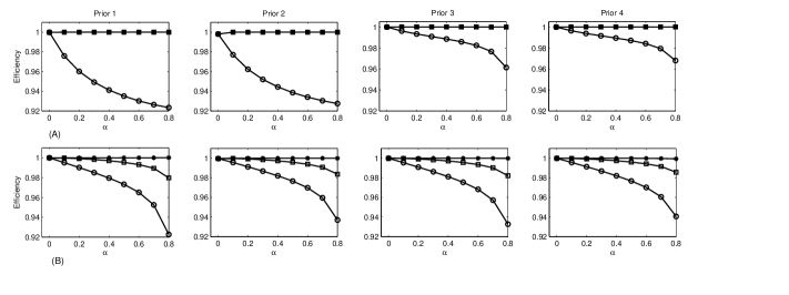
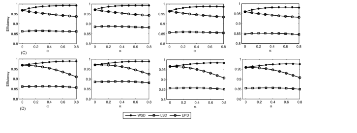
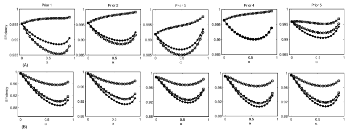
The Bayesian $D_{A}$-optimal design is obtained under three correlation structures, independent ($\alpha=0$), compound symmetric (CS) and AR(1). The proportions assigned to each treatment sequence by $D^{B}$ for varying $\alpha$ are plotted in Figure 1. It is noted (see Figure 1(A)) that under the independent correlation structure (i.e., $\alpha$ = 0), $D^{B}$ utilizes all the 16 sequences for priors 1, 3 and 4. In the case of prior 2 and $\alpha=0$, the sequences $\{BDCA,CBAD,BCDA,DBAC,AAAB,BBBA\}$ are left unused. As $\alpha$ increases for the CS structure, $D^{B}$ utilizes the sequences forming a LSD ($ADCB,BCDA,DABC,CBAD$) with almost 100% weightage and equal proportions to each. Under the AR(1) structure, $D^{B}$ uses only the first eight sequences (see Figure 1(B)). The efficiencies of the LSD, WSD and EPD with respect to $D^{B}$ are presented in Figure 2 (A). Note that under CS structure both LSD and WSD designs are as good as $D^{B}$, while EPD has lower efficiency, especially for priors 1 and 2. Efficiencies of LSD and WSD are constant with respect to $\alpha$ and also overlap. Under the AR(1) structure (see Figure 2 (B)), WSD is more efficient followed by LSD, and EPD performs worst. Note that performance of EPD also worsens as $\alpha$ increases. Efficiency comparisons are not much affected by the choice of the priors in the AR(1) case.

5.1.2 Full model: With carryover effect

It is observed from Figures 1 (C) and (D), for $\alpha=0$, under priors 2 and 3, $D^{B}$ utilizes all sequences except $\{BBBA\}$. For $\alpha=0$, prior 1: sequences $\{BBBA,CCDD,DDCC\}$ and prior 4: $\{BBBA,CCDD,DDCC,AABB\}$, are left unused , respectively. Under the CS and AR(1) structure, $D^{B}$ utilizes the first eight sequences with more than 70% of weight (see Figure 1 (C) and (D)), and as $\alpha$ increases the first eight sequences get more than 80% weight. It can be observed from Figure 2 (C) and (D) that WSD is most efficient as compared to LSD and EPD under all correlation structures. Also contrary to the reduced model, here the LSD performs worse (with about $85\%$ efficiency) than EPD. Efficiency comparisons are not much affected by the choice of the priors. Equation (14) in Theorem 1 in the appendix has been used to confirm the $D_{A}$-optimality of all Bayesian designs obtained for both reduced and full models.

Figure 1: Weights ($p_{\omega}$) versus the treatment sequences for different $\alpha$ values using priors 1-4 for the model parameters in Example 1. Treatment sequences labeled as $\{a,b,...,p\}$ correspond to the treatment sequences given in the design space $\Omega$ in Example 1 (Section 5.1). (A): Model with no carry over effect and correlation structure is CS (B): Model with no carry over effect and correlation structure is AR(1) (C): Model with carry over effect and correlation structure is CS (D): Model with carry over effect and correlation structure is AR(1)

Figure 2: Efficiencies of WSD, LSD and EPD compared with $D^{B}$ using priors 1-4 for the model parameters in Example 1, (A): Model with no carry over effect and correlation structure is CS (B): Model with no carry over effect and correlation structure is AR(1) (C): Model with carry over effect and correlation structure is CS (D): Model with carry over effect and correlation structure is AR(1)

5.2 Example 2: Two periods two treatments Poisson response trial

A crossover trial with two drugs given in two periods for controlling angina in 20 patients is considered. The count of attacks suffered by the patients is assumed to be a Poisson random variable. Treatment sequences $AB$ and $BA$ are used in the trial. However, we should note that this design does not permit the unbiased estimation of the treatment contrast under carryover effect (Jones and Kenward (2014)), though the estimates and corresponding confidence intervals may still be used to choose the prior distributions.

Reparametrizing the linear predictor $\eta_{ij}$ for this $2\times 2$ crossover design as done by Laska and Meisner (1985),

$$\eta_{ij}=\nu+\beta^{*}P+\tau^{*}T+\gamma^{*}C.$$

Here, $\tau^{*}=(\tau_{A}-\tau_{B})/2$, $\gamma^{*}=(\gamma_{A}-\gamma_{B})/2$, $\beta_{1}=0$ and $\beta_{2}=\beta^{*}$. The variables $P$ is coded 1 for period $2$ and zero otherwise, while $T,C=1$ for treatment $A$ and $-1$ for treatment $B$. It is assumed that carryover effect is zero in the first period. For a $2\times 2$ cross-over trial compound symmetric and AR(1) correlation structures are equal. Estimation of the parameters is again done by using PROC GENMOD in SAS software (SAS Institute Inc. (2003)). Point estimates and their 95% confidence intervals are listed in Table 2. Estimate of the correlation coefficient is $\alpha=0.0798$.

Table 2: Point estimates and confidence intervals for both reduced and full models for Poisson data in Example 2.

Parameter	Point estimate [95% Confidence interval]
	no carryover effect	with carryover effect
$\nu$	0.0493 [-0.4457  0.5444]	-0.0541 [-1.0405  0.9324]
$\beta^{*}$	-0.0011 [-0.4256  0.4234]	0.0541 [-0.4519  0.5600]
$\tau^{*}$	0.5664 [0.1006 1.0322]	0.6419 [-0.1036  1.3873]
$\gamma^{*}$	-	0.1494 [-0.8566  1.1553]

For a $2\times 2$ crossover design, the set of all possible treatment sequences is taken to be $\Omega=$ {$AB,BA,AA,BB$}. The Bayesian design with the $D_{A}$-optimal allocation of subjects to the treatment sequences {$AB,BA,AA,BB$} is denoted by $D^{B}$. The performance of $D^{B}$ is compared to $D_{I}=\{AB,BA,AA,BB\}$ and $D_{II}=$ {$AB,BA$}. Both $D_{I}$ and $D_{II}$ assigns equal allocation to each of their treatment sequences.

Following prior distributions for the model parameters were chosen:

• Cartesian product of 95% confidence intervals of parameters given in Table 2.

• Cartesian product of the nonnegative part of 95% confidence intervals of parameters given in Table 2.

• and 4: Independent multivariate normal distribution with mean vector as the point estimates of the parameters given in Table 2 and (for prior 3) the variance is 0.25, (for prior 4) the variance is 0.50.

5.2.1 Reduced model: No carryover effects

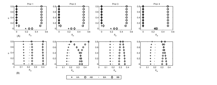
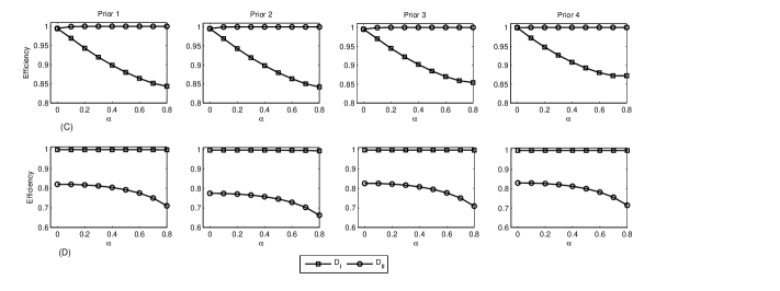
By observing Figure 3 (A), it is concluded that for $\alpha=0$, $D^{B}$ utilizes all sequences, for all priors. For $\alpha>0$, the Bayesian crossover design $D^{B}$ for the reduced model consists of sequences {$AB$, $BA$} with approximately equal weightage to each sequence, thus $D_{II}$ and $D^{B}$ are very similar under the reduced model. From Figure 3 (C) we see that $D_{II}$ is more efficient than $D_{I}$ and also the performance of $D_{I}$ worsens as $\alpha$ increases. Choices of the prior distributions do not effect the results. Also, the results matches with those for the normal response model for a $2\times 2$ crossover design (Laska and Meisner (1985)).

5.2.2 Full model: With carryover effects

Introducing crossover effects in the model, however changes the results completely except for the $\alpha=0$ case. The Bayesian crossover design $D^{B}$ for the full model now utilizes the sequences {$AA$, $AB$} and its dual. Proportions assigned to the treatment sequences are sensitive to the choice of the prior distribution as noted from Figure 3 (B). Figure 3 (D) shows that the design $D_{I}$ has efficiency values close to 1 and performs better than $D_{II}$. Also, $D_{II}$ is affected by increasing $\alpha$ (see Figure 3 (D)). For normal responses in case of a full model, similar results are noted by (Laska and Meisner (1985)). All designs obtained for the Poisson response here are verified to be $D_{A}$-optimal using Theorem 1 given in the Appendix.

Figure 3: Weights ($p_{\omega}$) assigned to each of the treatment sequences for different $\alpha$ values using priors 1-4 for the model parameters in Example 1 in (A): Model with no carry over effect (B): Model with carry over effect. Efficiency plots of designs $D_{I}$ and $D_{II}$ in (C): Model with no carry over effect (D): Model with carry over effect

5.3 Example 3: Three periods two treatment Gamma response trial

We consider a hypothetical gamma response trial with two treatments, $A$ and $B$ applied in three periods. For the $3\times 2$ crossover design the set of all possible treatment sequences is taken to be $\Omega=\{AAA,AAB,ABB,ABA,BBA,BAA,BAB,BBB\}$. The response is length of hospital stay which is assumed to follow a Gamma distribution. The Bayesian crossover design $D^{B}$ is determined by searching over $\Omega$. The linear predictor is again reparametrized as in Example 2, using $\tau^{*}=(\tau_{A}-\tau_{B})/2$, $\gamma^{*}=(\gamma_{A}-\gamma_{B})/2$, $\beta_{1}=0$, $\beta_{i}=\beta^{*}_{i-1},\,i=2,3$, and $T,C=1$ for treatment $A$ and $-1$ for treatment $B$,

$$\eta_{ij}=\nu+\beta_{1}^{*}P_{1}+\beta_{2}^{*}P_{2}+\tau^{*}T+\gamma^{*}C,$$

it is assumed that carryover effect is zero in the first period.

The data sets are simulated using the parameter values $(\nu,\beta_{1}^{*},\beta_{2}^{*},\tau^{*})=(0.50,0.15,0.20,0.25)$ for a reduced model and $(\nu,\beta_{1}^{*},\beta_{2}^{*},\tau^{*},\gamma^{*})=(0.50,0.20,0.30,0.25,0.15)$ for a full model. We have considered the treatment sequences $ABB$ and $BAA$ with the assignment of 10 subjects each to generate the data. Observations are assumed to be independent within the periods. The link function used is the reciprocal link and the shape parameter $\kappa$ is fixed at 2.0. Point estimates and corresponding confidence intervals of the parameters are calculated using PROC GENMOD procedure in SAS software (SAS Institute Inc. (2003)).

Following prior distributions for the model parameters are used to obtain the Bayesian optimal designs:

• Cartesian product of 95% confidence intervals of parameters given in Table 3.

• Cartesian product of the nonnegative part of 95% confidence intervals of parameters given in Table 3.

• $(\nu,\beta_{1}^{*},\beta_{2}^{*},\tau^{*},\gamma^{*})\in[-100,\;100]\times[-100,\;100]\times[-100,\;100]\times[-100,\;100]\times[-100,\;100]$.

• and 5: Independent multivariate normal distribution with mean vector as the point estimates of the parameters given in Table 3 and (for prior 4) the variance is 0.25, (for prior 5) the variance is 0.50.

For the reciprocal link function, we use the restriction $\eta_{ij}>0,i=1,\cdots,p,j=1,\cdots,n$. Prior 3 is a new prior considered here. Priors similar to prior 3 were not used in Examples 1 and 2, since such large values of parameters may have introduced singularity in the asymptotic variance covariance matrix of the parameter estimates.

The Bayesian design $D^{B}$ has been compared with the following designs:

• = $ABB,BAA,AAB,BBA$ with equal allocation to each treatment sequence.

• = $ABB,BAA$ with equal allocation to each treatment sequence.

• = $ABA,BAB,ABB,BAA$ with equal allocation to each treatment sequence.

Table 3: Point estimates and confidence intervals for both reduced and full models for Gamma response in Example 3.

Parameter	Point estimate [95% Confidence interval]
	no carryover effect	with carryover effect
$\nu$	0.5846 [ 0.3137  0.8556]	0.4653 [ 0.2671  0.6635]
$\beta_{1}^{*}$	0.1842 [ -0.0906  0.4591]	0.1360 [ -0.1814  0.4535]
$\beta_{2}^{*}$	0.2422 [ -0.0873  0.5717]	0.3661 [ 0.0818  0.6503]
$\tau^{*}$	0.2310 [ 0.0446   0.4173]	0.2830 [ -0.0150  0.5810]
$\gamma^{*}$	-	0.1178 [ -0.3020  0.5377]

5.3.1 Reduced model: No carryover effects

For log link function, asymptotic variance covariance matrix of parameter estimates does not depend on the model parameters, $\boldsymbol{\theta}$, as observed from the information matrix given in section 3.4 under the log link function. Thus results are similar to those in the normal response case. Under the CS structure, design {ABB, BAA} with equal proportions is the optimal design for direct treatment effect. Under AR(1) structure, optimal design utilizes the sequences $ABA$ and $BAB$ with equal proportions.

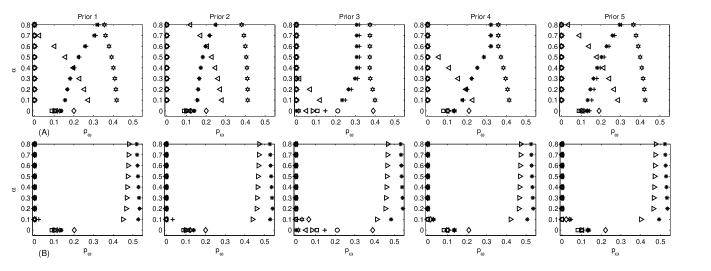
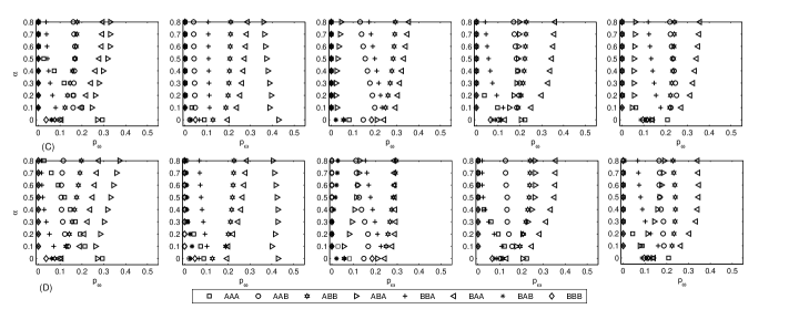
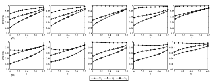
For reciprocal link function (see Figure 4 (A)), it is seen that for $\alpha=0$, all 8 sequences are utilized by $D^{B}$ except in the case of prior 3 (sequences $BAB,ABB$ are not used). For most of the positive $\alpha$ values and priors 1, 2 and 5, for the CS structure $D^{B}$ utilizes the sequences $\{BBA,BAB,BAA,ABB\}$. For priors 3 and 4 the sequence $BAA$ is left unused for high $\alpha$ values. Under each prior approximately 40% weightage is given to sequence $ABB$. With an increase in $\alpha$, weights on $BBA$ and $BAB$ also increase however weights on $BAA$ decrease. We also note that the weights on $BAA$ is sensitive to the prior used. From Figure 5 (A), it is noted that $D_{b}$ is most efficient, this is also true for normal responses.

Under AR(1) structure, $D^{B}$ utilizes the sequences $\{ABA,BAB\}$ with approximately 45% and 55% weightage, respectively, for each priors. These proportions are not affected by increasing $\alpha$ values (see Figure 4 (B)). From the efficiency plots (see Figure 5 (B)) design $D_{c}$ turns out to be the most efficient as compared to $D_{a}$ and $D_{b}$.

5.3.2 Full model: With carryover effects

For log link function again the results are similar to those in the normal response case. Under CS structure, $\{ABB,BAA\}$ is the optimal design and for AR(1) structure, optimal design is $\{ABB,AAB,BAA,BBA\}$ with more than 90% weightage given to the sequence $AAB$ and its dual.

For reciprocal link function, when $\alpha=0$, $D^{B}$ uses all sequences. Under both CS and AR(1) structures, $D^{B}$ uses the sequences $\{AAB,BAA,ABB,BAA,ABA\}$ (see Figure 4 (C) and (D)). It is observed that for smaller values of $\alpha$, the treatment sequence $AAA$ is included in the design. In Prior 1, the treatment sequence $AAA$ has approximate 30% weight for $\alpha=0$ and weightage decreases as $\alpha$ increases. From the efficiency plots (Figure 5 (C) and (D)), observe that design $D_{a}$ is the most efficient for CS correlation structures. Under the AR(1) structure, again $D_{a}$ performs well compared to other designs. Under prior 1 and 2, design $D_{c}$ has approximate equal efficiency as $D_{a}$ for $\alpha>0.4$. Note that, design $D_{a}$ is the optimal design for normal responses under AR(1) as noted in Laska and Meisner (1985).

Note again all designs obtained in this section are verified to be optimal using Theorem 1 given in the Appendix.

Figure 4: Weights ($p_{\omega}$) assigned to each treatment sequence for different $\alpha$ values using priors 1-5 for the model parameters in Example 3, (A): Model with no carry over effect and correlation structure is CS (B): Model with no carry over effect and correlation structure is AR(1) (C): Model with carry over effect and correlation structure is CS (D): Model with carry over effect and correlation structure is AR(1)

Figure 5: Efficiencies of designs $D_{a}$, $D_{b}$ and $D_{c}$ compared with $D^{B}$ using priors 1-5 for the model parameters in Example 3, (A): Model with no carry over effect and correlation structure is CS (B): Model with no carry over effect and correlation structure is AR(1) (C): Model with carry over effect and correlation structure is CS (D): Model with carry over effect and correlation structure is AR(1)

6 Sensitivity of designs to the assumed correlation structure

Till now in all our computations we assume that the working correlation (WC) matrix is equal to the true correlation (TC) matrix as defined in equation (7). In this section we investigate the effect of misspecifying the correlation on performance of designs. For illustration, Example 1 is used. There are two cases considered: Case (1): the working correlation structure is compound symmetric but the true correlation structure is AR(1), Case (2): the working correlation structure is AR(1) but the true correlation structure is compound symmetric. Prior 1 used before in Example 1 is assigned to the regression parameters.

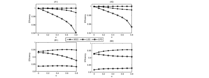
First we consider a model without the carryover effect. The Bayesian $D_{A}$-optimal design, $D^{B}$, is found using equation (6) in equation (10). $D^{B}$ utilizes the sequences forming a LSD under both cases 1 and 2. Under misspecification, performance of WSD is affected very slightly (see Figure 6 (A1) and (A2)), EPD performs the worst and its performance worsens with $\alpha$.. However, for the TC=WC case, we had noted earlier that both LSD and WSD are equally efficient. Thus, misspecification under the reduced model case, has a slight adverse effect on the performance of the WSD but not the LSD.

For the model with carryover effect, for both cases 1 and 2, $D^{B}$ utilizes the first 8 sequences with more than 70% weights (this is consistent with results obtained under TC = WC). Though the performance of WSD is affected it is still the most efficient compared to EPD and LSD (see Figure 6 (B1) and (B2)), while LSD is the worst.

Figure 6: Efficiency plots of WSD, LSD and EPD compared to $D^{B}$ when true correlation (TC) and working correlation (WC) are not equal (A1) Model without carryover effect and WC = compound symmetric (CS), TC = autoregressive (AR(1)), (A2) Model without carryover effect and WC = AR(1), TC = CS, (B1) Model with carryover effect and WC = CS, TC = AR(1), (B2) Model without carryover effect and WC = AR(1), TC = CS

7 Prior distributions on $\alpha$ and its effect on design performances

Designs obtained so far are based on some fixed values of $\alpha$. In this section, we validate the performance of the optimal designs using priors on $\alpha$. For illustration purpose, we consider the two periods two treatments Poisson response model with carry over effect from Example 2. Prior 1 of Example 2 is chosen for the parameters involved in the linear predictor. The estimate of $\alpha$ using the data given in Example 2 is 0.0798. Based on this information we use the following set of priors covering the value 0.0789.

• (i) Uniform(0, 0.2) (ii) Uniform(0, 0.5) (iii) Uniform(0, 0.8) (iv) Uniform(0, 1)

• (i) Beta(2, 38) (ii) Beta(4, 12) (iii) Beta(6, 10) (iv) Beta(5, 5).

The first four uniform and beta priors (i-iv) are chosen such that they have similar ranges, i.e., the range of uniform (i) is similar to beta prior (i) and so on. They are also chosen to look at the effect of increasing uncertainty of the prior information on the designs. Uniform and Beta priors have been used before by Spiegelhalter (2001) and Singh and Mukhopadhyay (2016) for the correlation parameter of cluster randomized trials.

The ${D_{A}}$-optimal Bayesian criterion defined in equation (10) changes to the design which minimizes

$$\Psi(\mathfrak{B^{*}},\zeta)=\int_{\mathfrak{B^{*}}}\Lambda(\zeta,\boldsymbol{\theta},\alpha)\,dF(\boldsymbol{\theta},\alpha),$$ (13)

where $\mathfrak{B^{*}}\subset\mathbb{R}^{m}\times[0,1]$ is the parameter space of parameter vector $(\boldsymbol{\theta},\alpha)$ and $F(\boldsymbol{\theta},\alpha)$ is a proper prior distribution for $(\boldsymbol{\theta},\alpha)$. Optimal proportions of $D^{B}$ using the above criterion for different priors of $\alpha$ are given in Table 4. As noted before in Example 2, design $D_{I}=\{AA,AB,BA,BB\}$ with equal proportions performs well as compared to the Bayesian $D_{A}$-optimal design with efficiency values approximately equal to 1. From Table 4, it is observed that optimal proportions are slightly sensitive to the choice of priors. For example see the optimal allocations corresponding to Uniform(0, 0.2) and Beta(5, 5) priors. Overall, we may conclude that there is not much change in the results when we use a prior for $\alpha$ instead of some fixed values.

Table 4: Optimal allocation of $D^{B}$ under different priors for $\alpha$ and efficiency values of $D_{I}$ (Section 7).

	$p_{\omega}$
Prior	AA	AB	BA	BB	Efficiency
Uni(0, 0.2)	0.1520	0.2700	0.2133	0.3647	0.988
Uni(0, 0.5)	0.1506	0.2716	0.2161	0.3617	0.988
Uni(0, 0.8)	0.1503	0.2744	0.2167	0.3586	0.988
Uni(0, 1.0)	0.1515	0.2766	0.2124	0.3595	0.988
Beta(2, 38)	0.2000	0.2000	0.3000	0.3000	0.996
Beta(4, 12)	0.1997	0.1992	0.3005	0.3006	0.995
Beta(6, 10)	0.2060	0.1986	0.2908	0.3047	0.991
Beta(5, 5)	0.1843	0.1841	0.2876	0.3440	0.989

8 Computer programs used to obtain the optimal designs and estimate the parameters

Approximation of the multidimensional integrals of the objective functions in equations (10) and (13) to obtain the optimal designs is done with Latin Hypercube Sampling (LHS). For uniform priors, we use the average of (10) and (13) across 100-point discrete samples using LHS as the approximate solution of (10) and (13), respectively. When $\boldsymbol{\theta}$ has a Gaussian distribution, Latin Hypercube Sampling from Gaussian fields is used (for more details see Stein (1987)). A MATLAB function lhsdesign is used to sample points from the parameter space. To obtain the optimal proportions of subjects ($p_{\omega}$) assigned to treatment ($\omega$), fmincon function in MATLAB is used. The fmincon algorithm finds a minimum of a constrained nonlinear multivariable function, and by default is based on the Sequential Quadratic Programming algorithm. For more details please see the link http://in.mathworks.com/help/optim/ug/fmincon.html$\#$description. A genetic algorithm (GA function in MATLAB) verifies the results obtained from the fmincon. The estimation and the estimated confidence intervals of model parameters are done using GENMOD procedure in SAS (SAS Institute Inc. (2003)).

Note: All MATLAB and SAS programs are available to the readers upon request from the first author of this article.

9 Concluding Remarks

Crossover designs are popular as designs of choice in many clinical and pharmaceutical trials for comparing treatments. However, very often in these situations the response does not follow the usual assumptions of normality, and generalized linear models have to be used to model the data. In this article, we address the designing of such crossover trials when a GLM is fitted. Since the designs are dependent on the model parameters, Bayesian designs are proposed. Comparing our main results based on GLMs with those of normal response models, we see that they are quite similar in many cases.

The main results on the estimation of direct treatment effects using the proposed $D_{A}$-optimal Bayesian designs ($D^{B}$) are summarized below.

• For $t=p=4$ when the response is binary : Williams design is as efficient as $D^{B}$ and is seen to perform the best under both CS and AR(1) correlation structures for a reduced as well as a full model.

• For $p=t=2$ when the response is Poisson distributed: Design {$AB,BA$} has the highest efficiency in a reduced model framework while for a full model, design {$AB,BA,AA,BB$} is most efficient. Both designs have equivalent efficiency as $D^{B}$ for the respective models.

• For $p=3,t=2$ when the response is Gamma distributed: Under log link function, $D_{A}$-optimal Bayesian designs are same as in case of normal responses.

  For reciprocal link function, under reduced model, design $D_{b}$ (treatment sequences $\{ABB$, $BAA\}$ with equal proportions), perform as well as $D^{B}$ under the CS correlation structure, while for AR(1) correlation structure, design $D_{c}$ (treatment sequences $\{ABA,BAB,$ $ABB,BAA\}$ with equal proportions) has the equal efficiency as $D^{B}$.

  In case of full model, design $D_{a}$ (treatment sequences $\{ABB,BAA,AAB,BBA\}$ with equal proportions) is equally efficient as $D^{B}$, and performs better than $D_{b}$ and $D_{c}$.

In many biological experiments while studying the effect of drugs, the response measured may not be binary in nature but say ordinal. As an example consider a $3\times 3$ crossover trial (cited by Jones and Kenward (2014)) where the effect of three treatments on the amount of patient relief is studied. The response obtained is categorized as none, moderate or complete, making it ordinal in nature with three categories. Thus, there is a need to address optimal crossover deigns not just for binary models but also for multi categorical responses. In these cases, instead of the logit link, a generalized logit or a proportional odds model may be used. Also, other than the correlation between measurements from the same subject we would have to consider the relation between response categories. Jones and Kenward (2014) discusses modeling of ordinal data using the GEE approach. In future, we are interested to study D-optimal Bayesian designs for such multicategorical models.

Appendix

Consider a finitely supported approximate crossover design with $k$ treatment sequences. The design can be expressed in the form of a probability measure as follows:

$$\zeta=\begin{Bmatrix}\omega_{1}&\omega_{2}&\dots&\omega_{k}\\ p_{\omega_{1}}&p_{\omega_{2}}&\dots&p_{\omega_{k}}\end{Bmatrix},$$

where $\omega_{i}\in\Omega$ (set of all treatment sequences considered) and $p_{\omega_{i}}$ is the proportion of subjects assign to treatment sequence $\omega_{i}$ such that $p_{\omega_{i}}\geq 0$ and $\sum_{i=1}^{k}p_{\omega_{i}}=1$, for $i=1,\cdots,k$. Let $M=M(\zeta,\boldsymbol{\theta})$ denotes the asymptotic information matrix of estimates of the parameter vector $\boldsymbol{\theta}$. This in turn is the reciprocal of the variance-covariance matrix defined in equation (7). If the interest is in the estimation of a linear combination of the parameters of the form $\lambda=W^{\prime}\boldsymbol{\theta}$, where $W$ is a $m\times s$ matrix with rank $s\leq m$. The information matrix of $\lambda$ for a design $\zeta$ is given by $C=C(\zeta,\lambda)=(W^{\prime}M^{-1}W)^{-1}$. Next theorem insures the optimality of designs obtain for the estimation of $\lambda$ under the prior distribution of $\boldsymbol{\theta}$.

Theorem 1

Under the GEE model considered for the linear predictor, link function and working correlation, the following conditions for a continuous design $\zeta^{*}$ are equivalent:

• $\zeta^{*}$ minimizes $\Psi(\mathfrak{B},\zeta,\alpha)$ defined in equation (10), $\forall$  $\zeta\in\chi$, where $\chi$ is the set of all possible designs.

• $\zeta^{*}$ satisfies the following condition:

  $$E_{F}\left[\mbox{tr}\left(M(\zeta^{*},\boldsymbol{\theta})^{-1}WCW^{\prime}M(\zeta^{*},\boldsymbol{\theta})^{-1}\right)M(\zeta_{\omega},\boldsymbol{\theta})\right]\leq s\;\forall\;\omega\in\Omega,$$ (14)

  where $F$ is the prior distribution of $\boldsymbol{\theta}$ and $M(\zeta_{\omega},\boldsymbol{\theta})$ is the information matrix with respect to the design $\zeta_{\omega}$ having unit mass at single treatment sequence $\omega$. Equality in equation (14) is achieved if any $\omega$ in the Bayesian $D_{A}$-optimal design is inserted.

Proof of this theorem follows directly from Theorem 3.1 of Pettersson (2005). These optimal designs are known as average $D_{A}$-optimal designs. A similar equivalence theorem is proved and used by Woods and Van de Ven (2011) to show the optimality of blocked designs with non-normal responses. Expressions of matrix $W$, $\boldsymbol{\theta}$ and respective ranks for examples used in this article are:

• Example 1

  $$W^{\prime}=\begin{bmatrix}0&0&0&0&1&0&0&0&0&0\\ 0&0&0&0&0&1&0&0&0&0\\ 0&0&0&0&0&0&1&0&0&0\end{bmatrix}$$

  $\boldsymbol{\theta}=(\nu,\beta_{1}^{*},\beta_{2}^{*},\beta_{3}^{*},\tau_{1}^{*},\tau_{2}^{*},\tau_{3}^{*},\gamma_{1}^{*},\gamma_{2}^{*},\gamma_{3}^{*})^{\prime}$ and $s$ = 3.

• Example 2

  $$W^{\prime}=\begin{bmatrix}0&0&1&0\end{bmatrix}$$

  $\boldsymbol{\theta}=(\nu,\beta^{*},\tau^{*},\gamma^{*})^{\prime}$ and $s$ = 1.

• Example 3

  $$W^{\prime}=\begin{bmatrix}0&0&0&1&0\end{bmatrix}$$

  $\boldsymbol{\theta}=(\nu,\beta_{1}^{*},\beta_{2}^{*},\tau^{*},\gamma^{*})^{\prime}$ and $s$ = 1.

Acknowledgement: Mr. Satya Prakash Singh wishes to thank University Grant Commission (UGC), India, for the award of a research fellowship. The work of Siuli Mukhopadhyay was supported by the IRCC seed funding under the health care consortium [Grant Number: 15IRSGHC004]. These supports are gratefully acknowledged.

References

- Atkinson et al. (2007) Atkinson, A. C., Donev, A. N., Tobias, R. D., 2007. Optimum Experimental Designs, With SAS. Oxford University Press, Oxford.
- Baily and Kunert (2006) Baily, R. A., Kunert, J., 2006. On optimal crossover designs when carryover effects are proportional to direct effects. Biometrika 93 (3), 613–625.
- Bandyopadhyay et al. (2009) Bandyopadhyay, U., Biswas, A., Mukherjee, S., 2009. Adaptive two-treatment two-period crossover design for binary treatment responses incorporating carry-over effects. Statistical Methods and Applications 18 (1), 13–33.
- Bose and Dey (2009) Bose, M., Dey, A., 2009. Optimal Crossover Designs. World Scientific, Singapore.
- Bose and Dey (2013) Bose, M., Dey, A., 2013. Developments in crossover designs. http://www.isid.ac.in/ statmath/2013/isid201307.pdf.
- Carriere and Huang (2000) Carriere, K. C., Huang, R., 2000. Crossover designs for two-treatment clinical trials. Journal of Statistical Planning and Inference 87, 125–134.
- Carrire and Reinsel (1993) Carrire, K. C., Reinsel, G. C., 1993. Optimal two-period repeated measurement designs with two or more treatments. Biometrika 80 (4), 924–929.
- Chaloner and Larntz (1989) Chaloner, K., Larntz, K., 1989. Optimal bayesian design applied to logistic regression experiments. Journal of Statistical Planning and Inference 21, 191–208.
- Cheng and Wu (1980) Cheng, C. S., Wu, C. F., 1980. Balanced repeated measurements designs. Annals of Statistics 8 (6), 1272–1283.
- Cochran (1939) Cochran, W. G., 1939. Long-term agricultural experiments. Journal of the Royal Statistical Society 6 (2), 104–148.
- Dette and Sperlich (1994) Dette, H., Sperlich, S., 1994. A note on bayesian -optimal designs for a generalization of the exponential growth model. South African Statistical Journal 28, 103–117.
- Dror and Steinberg (2006) Dror, H. A., Steinberg, D. M., 2006. Robust experimental design for multivariate generalized linear models. Technometrics 48 (4), 520–529.
- Faddy et al. (2009) Faddy, M., Graves, N., Pettitt, A., 2009. Modeling length of stay in hospital and other right skewed data: Comparison of phase-type, gamma and log-noraml distributions. Value in Health 12 (2), 309–314.
- Forster (1992) Forster, J. J., 1992. A bayesian approach to the analysis of binary crossover data. Journal of the Royal Statistical Society. Series D (The Statistician) 43 (1), 13–29.
- Hedayat and Afsarinejad (1975) Hedayat, A., Afsarinejad, K., 1975. Repeated measurements designs, I. In A Survey of Statistical Designs and Linear Models, J. N. srivastava Edition. Chapman and Hall, Amsterdam: North-Holland, pp. 229-242.
- Hedayat and Afsarinejad (1978) Hedayat, A., Afsarinejad, K., 1978. Repeated measurements designs, II. Annals of Statistics 6 (3), 619–628.
- Jones and Kenward (2014) Jones, B., Kenward, M., 2014. Design and Analysis of Cross-over Trials, 3rd Edition. CRC Press, London.
- Kempton et al. (2001) Kempton, R. A., Ferris, S. J., David, O., 2001. Optimal change-over designs when carry-over effects are proportional to direct effects of treatments. Biometrika 88 (2), 391–399.
- Kenward and Jones (1992) Kenward, M. G., Jones, B., 1992. Alternative approaches to the analysis of binary and categorical repeated measurements. Journal of Biopharmaceutical Statistics 2 (2), 137–170.
- Kushner (1997) Kushner, H. B., 1997. Optimal repeated measurements designs: The linear optimality equations. The Annals of Statistics 25 (6), 2328–2344.
- Kushner (1998) Kushner, H. B., 1998. Optimal and efficient repeated-measurements designs for uncorrelated observations. Journal of the American Statistical Association 93 (443), 1176–1187.
- Laska et al. (1983) Laska, E., Meisner, M., Kushner, H. B., 1983. Optimal crossover designs in the presence of carryover effects. Biometrics 39 (4), 1087–1091.
- Laska and Meisner (1985) Laska, E. M., Meisner, M., 1985. A variational approach to optimal two-treatment crossover designs: Application to carryover-effect models. Journal of the American Statistical Association 80 (391), 704–710.
- Lawson (2014) Lawson, J., 2014. Design and Analysis of Experiments with R. Chapman and Hall, CRC Press.
- Layard and Arvesen (1978) Layard, M. W. J., Arvesen, J. N., 1978. Analysis of Poisson data in crossover experimental designs. Biometrics 34 (3), 421–428.
- Li et al. (2015) Li, K., Zheng, W., Mingyao, A., 2015. Optimal designs for the proportional interference model. The Annals of Statistics 43 (4), 1596–1616.
- Liang and Zeger (1986) Liang, K. Y., Zeger, S. L., 1986. Longitudinal data analysis using generalized linear models. Biometrika 73 (1), 13–22.
- Mylona et al. (2014) Mylona, K., Goos, P., Jones, B., 2014. Optimal design of blocked and split-plot experiments for fixed effects and variance component estimation. Technometrics 56 (2), 132–144.
- Patterson and Lucas (1959) Patterson, H. D., Lucas, H. L., 1959. Extra-period change-over designs. Biometrics 15 (1), 116–132.
- Pettersson (2005) Pettersson, H., 2005. Optimal design in average for inference in generalized linear models. Statistical Papers 46, 79–100.
- SAS Institute Inc. (2003) SAS Institute Inc., 2003. SAS/STAT Software, Version 9.2. Cary, NC.
- Senn (2002) Senn, S., 2002. Cross-Over Trials in Clinical Research, 2nd Edition. Wiley, New York.
- Singh and Mukhopadhyay (2016) Singh, S. P., Mukhopadhyay, S., 2016. Bayesian optimal cluster designs. Statistical Methodology 32, 36–52.
- Spiegelhalter (2001) Spiegelhalter, D. J., 2001. Bayesian methods for cluster randomized trials with continuous responses. Statistics in Medicine 20, 435–452.
- Stein (1987) Stein, M., 1987. Large sample properties of simulations using latin hypercube sampling. Technometrics 29 (2), 143–151.
- Stufken (1991) Stufken, J., 1991. Some families of optimal and efficient repeated measurements designs. Journal of Statistical Planning and Inference 27 (1), 75–83.
- Waterhouse et al. (2006) Waterhouse, T. H., Eccleston, J. A., Duffull, S. B., 2006. Optimal crossover designs for logistic regression models in pharmacodynamics. Journal of Biopharmaceutical Statistics 16, 881–894.
- Williams (1949) Williams, E. J., 1949. Experimental designs balanced for the estimation of residual effects of treatments. Australian Journal of Scientific Research 2 (3), 149–168.
- Woods et al. (2006) Woods, D. C., Lewisa, S. M., Eccleston, J. A., Russell, K. G., 2006. Designs for generalized linear models with several variables and model uncertainty. Technometrics 48 (2), 284–292.
- Woods and Van de Ven (2011) Woods, D. C., Van de Ven, P. M., 2011. Blocked designs for experiments with correlated non-normal response. Technometrics 53, 173–182.
- Zeger et al. (1988) Zeger, S. L., Liang, K. Y., Albert, P. S., 1988. Models for longitudinal data: A generalized estimating equation approach. Journal of the American Statistical Association 44 (4), 1049–1060.
- Zheng (2013) Zheng, W., 2013. Optimal crossover designs for the proportional model. The Annals of Statistics 41 (4), 2218–2235.