What do we know about cosmography

Abstract

In the present paper, we investigate the cosmographic problem using the bias-variance tradeoff. We find that both the $z$-redshift and $y=z/(1+z)$-redshift can present a small bias estimation. It means that the cosmography can describe the supernova data more accurately. Minimizing risk, it suggests that cosmography up to the 2 order is the best approximation. Forecasting the constraint from future measurements, we find that future supernova and redshift drift can significantly improve the constraint, thus having a potential to solve the cosmographic problem. We also exploit the values of cosmography on the deceleration parameter and equation of state of dark energy $w(z)$. We find that supernova cosmography cannot give stable estimations on them. However, many useful information were obtained, such as that the cosmography favors a complicated dark energy with varying $w(z)$, and the derivative $\textmd{d}w/\textmd{d}z<0$ for low redshift. The cosmography is helpful to model the dark energy.

I Introduction

Cosmic accelerating expansion is a landmark cosmological discovery in recent decades. Till now, a number of dynamical mechanisms have been proposed to explain this mysterious cosmological phenomenon. However, its natural essence is still not known to us. The theoretical attempts include dark energy, or modified gravity, or violation of cosmological principle. Thereinto, the first paradigm believes that an exotic cosmic component called dark energy probably exists in a form of the cosmological constant Carroll et al. (1992), or scalar field Caldwell et al. (2003); Feng et al. (2005) and possesses a negative pressure to drive the cosmic acceleration. The modified gravities do not need an exotic component but a modification to the general relativity theory Barrow and Cotsakis (1988); Dvali et al. (2000). While violation of cosmological principle is usually in form of the inhomogeneous Lemaître-Tolman-Bondi void model Lemaître (1933); Tolman (1934); Bondi (1947).

Different from above dynamical templates, cosmic kinematics is a more moderate approach in understanding this acceleration. It only highlights a homogeneous and isotropic universe at the large scale. In this family, kinematic parameters independent of the cosmic dynamical models become very essential. For example, the scale factor $a(t)$ directly describes how the universe evolves over time. The deceleration factor can immediately map the decelerating or accelerating expansion of the universe. Collecting some kinematic parameters, the authors in Refs. Chiba and Nakamura (1998); Visser (2004) created the cosmography via Taylor expansion of the luminosity distance over the redshift $z$. Mathematically, this expansion should be performed near a small quantity, i.e. the low redshift. Using the standard complex variable theory, Cattoën and Visser Cattoën and Visser (2007) demonstrated that convergence radius of Taylor expansion over redshift $z$ is at most $|z|=1$. For high redshift $z>1$, it fails to convergence. Nevertheless, many observations focus on the high redshift region. For example, the supernova in joint light-curve analysis (JLA) compilation can span the redshift region up to 1.3; the cosmic microwave background (CMB) even can retrospect to the very early universe at $z\sim 1100$. To legitimate the expansion at high redshift, they introduced an improved redshift parametrization $y=z/(1+z)$ Cattoën and Visser (2007). Thus, cosmography in the $y-$based expansion is mathematically safe and useful, because of $0<y<1$, even for the high redshift. Later, some other fashions of redshift were also proposed Aviles et al. (2012).

When confronting with observational data, the cosmography study encounter some difficulties. Initially, the SNIa data were used to fit with the cosmography Cattoën and Visser (2008); Capozziello et al. (2011). Then some auxiliary data sets Xia et al. (2012) were also considered. The output indicated that fewer series truncation lead to smaller errors but worse estimation; and more terms lead to more accurate approximation but bigger errors. That is, cosmography is in the dilemma between accuracy and precision. The crisis naturally turns to the question of where is the “sweet spot”, i.e., the most optimized series truncation. In previous work Cattoën and Visser (2008); Vitagliano et al. (2010); Xia et al. (2012), they found that estimation up to the snap term is meaningless in the light of F-test. For the $y$-redshift, it presents bigger errors of the parameters Cattoën and Visser (2008). In spite of different observational data sets were used, most of the results were consistent. Recent work Lazkoz et al. (2013) investigated the cosmography using the baryon acoustic oscillations (BAO) only. From the simulated Euclid-like BAO survey, they found that future BAO observation also favored a best cosmography with a jerk term. Because it only requires the homogeneity and isotropy of the universe, cosmography was frequently used to deduce or test the cosmological models. Recently, it was used to test the $\Lambda$CDM model Busti et al. (2015), but it turned out that the parameter $j_{0}\neq 1$ is ambiguous for different orders of expansion, which is not enough to test it. Reconstructing dark energy in $f(R)$ gravities, they found that there exists extra free parameters, which cannot be constrained by the cosmography. The analysis was based on the mock data generated by a unified error of magnitude $\sigma_{\mu}=0.15$. In the following text, we will test the constraint of these mock data with flat errors. Following the work in Ref. Busti et al. (2015), these mock data were generated assuming the same redshift distribution as the Union 2.1 catalogue Suzuki et al. (2012), but under the fiducial model from the best-fit ones by JLA data.

Although the cosmography has been widely investigated, there still left a lot of questions. On the one hand, we do not present a repetitive work using more data, but numerically excavate more detailed information about the accuracy and precision in convergence problem. The new approach we use is the bias-variance tradeoff. Moreover, we will try to investigate whether future measurement can solve the serious convergence issue. On the other hand, before the use of cosmography, we should make certain what information it can provide and what it cannot provide.

Although many types of observational data were used to fit the cosmography, our goal in this paper is to understand the convergence problem from another side, i.e., the geometric or dynamical measurement. Future surveys with high-precision may present a different constraint. To understand above questions, we need the help of future WFIRST-like supernova observation and a dynamical survey redshift drift. Different from the geometric measurement, the redshift drift is desired to measure the secular variation of $\dot{a}(t)$ Sandage (1962). In contrast, geometric observation usually measure an integral of $\dot{a}(t)$. Interestingly, this concept is also independent of any cosmological model, requiring only the Friedmann-Robertson-Walker universe. Taking advantage of the capacity of E-ELT Liske et al. (2008a, b); Corasaniti et al. (2007), numerous works agreed that this future probe could provide excellent contribution to understand the cosmic dynamics, such as the dark energy Zhang and Liu (2014); Geng et al. (2015) or modified gravity models Li et al. (2013). More importantly, it can be extended to test the fundamental Copernican principle Uzan et al. (2008) and the cosmic acceleration Yu et al. (2014). However, study of the redshift drift on kinematics has been scarce.

This paper is organized as follows: In Section II, we introduce the cosmography. And in Section III we present the observational data. According to the goals introduced above, we analyze the problem of cosmography in Section IV, and explore its values in Section V. Finally, in Section VI conclusion and discussion are drawn.

II Cosmography

Cosmography is an artful combination of kinematic parameters via the Taylor expansion with a hypothesis of large-scale homogeneity and isotropy. In this framework, introduction of the interested cosmographic parameters is appropriate.

Hubble parameter

$$H(t)=+\frac{1}{a}\frac{da}{dt}$$ (1)

accurately connects the cosmological models with observational data.

Deceleration parameter

$$q(t)=-\frac{1}{a}\frac{d^{2}a}{dt^{2}}\left[\frac{1}{a}\frac{da}{dt}\right]^{-2}$$ (2)

directly represents the decelerating or accelerating expansion of the universe.

Jerk parameter

$$j(t)=+\frac{1}{a}\frac{d^{3}a}{dt^{3}}\left[\frac{1}{a}\frac{da}{dt}\right]^{-3}$$ (3)

and snap parameter

$$s(t)=+\frac{1}{a}\frac{d^{4}a}{dt^{4}}\left[\frac{1}{a}\frac{da}{dt}\right]^{-4}$$ (4)

are often used as a geometrical diagnostic of dark energy models Sahni et al. (2003); Alam et al. (2003). An important feature should be announced is that jerk has being a traditional tool to test the spatially flat cosmological constant dark energy model in which $j(z)=1$ all time.

Lerk parameter

$$l(t)=+\frac{1}{a}\frac{d^{5}a}{dt^{5}}\left[\frac{1}{a}\frac{da}{dt}\right]^{-5}$$ (5)

is an higher order parameter to indicate the cosmic expansion.

With above preparation, Hubble parameter in the cosmography can be expressed as Chiba and Nakamura (1998); Capozziello et al. (2011)

$$H(z) = H_{0}+\frac{dH}{dz}\Big{|}_{z=0}z+\frac{1}{2!}\frac{d^{2}H}{dz^{2}}\Big{|}_{z=0}z^{2}+\frac{1}{3!}\frac{d^{3}H}{dz^{3}}\Big{|}_{z=0}z^{3}+\cdots$$ (6)

$$= H_{0}\Big{[}1+(1+q_{0})z+\frac{1}{2}(-q_{0}^{2}+j_{0})z^{2}$$

$$+ \frac{1}{6}(3q_{0}^{2}+3q_{0}^{3}-4q_{0}j_{0}-3j_{0}-s_{0})z^{3}$$

$$+ \frac{1}{24}(-12q_{0}^{2}-24q_{0}^{3}-15q_{0}^{4}+32q_{0}j_{0}+25q_{0}^{2}j_{0}$$

$$+ 7q_{0}s_{0}+12j_{0}-4j_{0}^{2}+8s_{0}+l_{0})z^{4}\Big{]}+\cdots$$

where the subscript “0” indicates cosmographic parameters evaluated at the present epoch. According to the differential relations with Hubble parameter, luminosity distance in the cosmography study can be conveniently expressed as Cattoën and Visser (2007); Capozziello et al. (2011)

$$d_{L}^{\textmd{cos}}(z)=z+\mathcal{C}_{1}z^{2}+\mathcal{C}_{2}z^{3}+\mathcal{C}_{3}z^{4}+\mathcal{C}_{4}z^{5},$$ (7)

where

$$\mathcal{C}_{1} = \frac{1}{2}(1-q_{0})$$

$$\mathcal{C}_{2} = -\frac{1}{6}(1-q_{0}-3q_{0}^{2}+j_{0})$$

$$\mathcal{C}_{3} = \frac{1}{24}(2-2q_{0}-15q_{0}^{2}-15q_{0}^{3}+5j_{0}+10q_{0}j_{0}+s_{0})$$

$$\mathcal{C}_{4} = \frac{1}{120}(-6+6q_{0}+81q_{0}^{2}+165q_{0}^{3}+105q_{0}^{4}$$ (8)

$$+ 10j_{0}^{2}-27j_{0}-110q_{0}j_{0}-105q_{0}^{2}j_{0}-15q_{0}s_{0}$$

$$- 11s_{0}-l_{0}),$$

As introduced above, cosmography at high redshift $z>1$ fails to converge. To solve this trouble, a $y$-redshift hence introduced Cattoën and Visser (2007)

$$y=\frac{z}{1+z}.$$ (9)

For the new redshift, we can simplify it as $y=1-a(t)$. Obviously, it is $0<y<1$ for the current observational data. One benefit from the $y$-redshift is that it can extend the expansion to high redshift region. This is important for the cosmography study. The reason is that cosmography in Eq. (7) is theoretically valid for redshift $z<1$. While with the import of $y$-redshift, many observational data such as supernova with higher redshift and even CMB, can be used to fit and study the cosmography. For example, it is reduced to $y=0.56$ for the supernova at max redshift $z=1.3$ in JLA compilation. Moreover, its value is $y=0.999$ which guarantees the safe use of the early CMB data. As described in Ref. Cattoën and Visser (2007), it even can extrapolate back to the big bang. The other physical significance is $y$ redshift also can back to the future universe, but breaks down at $y=-1$. In the $y$-redshift space, the luminosity distance is

$$d_{L}^{\textmd{cos}}(y)=y+\mathcal{C}_{1}y^{2}+\mathcal{C}_{2}y^{3}+\mathcal{C}_{3}y^{4}+\mathcal{C}_{4}y^{5},$$ (10)

with

$$\mathcal{C}_{1} = \frac{1}{2}(3-q_{0})$$

$$\mathcal{C}_{2} = \frac{1}{6}(11-5q_{0}+3q_{0}^{2}-j_{0})$$

$$\mathcal{C}_{3} = \frac{1}{24}(50-26q_{0}+21q_{0}^{2}-15q_{0}^{3}-7j_{0}+10q_{0}j_{0}+s_{0})$$

$$\mathcal{C}_{4} = \frac{1}{120}(274-154q_{0}+141q_{0}^{2}-135q_{0}^{3}+105q_{0}^{4}$$ (11)

$$+ 10j_{0}^{2}-47j_{0}+90q_{0}j_{0}-105q_{0}^{2}j_{0}-15q_{0}s_{0}$$

$$+ 9s_{0}-l_{0}).$$

In following analysis, one we should do is to test the improvement of $y$-redshift.

In our cosmographic study, we need the help of dynamical redshift drift. The story should start from the redshift.

In an expanding universe, we observe at time $t_{0}$ a signal emitted by a source at $t_{\mathrm{em}}$. The source’s redshift can be represented through the cosmic scale factor

$$z(t_{0})=\frac{a(t_{0})}{a(t_{\mathrm{em}})}-1.$$ (12)

Over the observer’s time interval $\Delta t_{0}$, the source’s redshift becomes

$$z(t_{0}+\Delta t_{0})=\frac{a(t_{0}+\Delta t_{0})}{a(t_{\mathrm{em}}+\Delta t_{\mathrm{em}})}-1,$$ (13)

where $\Delta t_{\mathrm{em}}$ is the time interval-scale for the source to emit another signal. It should satisfy $\Delta t_{\mathrm{em}}=\Delta t_{0}/(1+z)$. As a consequence, the observed redshift variation of the source is

$$\Delta z=\frac{a(t_{0}+\Delta t_{0})}{a(t_{\mathrm{em}}+\Delta t_{\mathrm{em}})}-\frac{a(t_{0})}{a(t_{\mathrm{em}})}.$$ (14)

Taking the first order approximation to Eq. (14), physical interpretation of redshift drift can be exposed in

$$\Delta z\approx\left[\frac{\dot{a}(t_{0})-\dot{a}(t_{\mathrm{em}})}{a(t_{\mathrm{em}})}\right]\Delta t_{0},$$ (15)

where dot denotes the derivative with respect to cosmic time. Obviously, we should note that the secular redshift drift monitor a variation of $\dot{a}$ during the evolution of the universe. For the distance measurement, it commonly extracts information content via the integral of a variant of $\dot{a}$. Theoretically, the Hubble parameter, a function of $\dot{a}$ may be more effective to probe the cosmic expansion information. However, its acquisition in observational cosmology currently is indirect from the differential ages of galaxies Jimenez and Loeb (2008); Simon et al. (2005); Stern et al. (2010), from the BAO peaks in the galaxy power spectrum Gaztanaga et al. (2009); Moresco et al. (2012), or from the BAO peaks using the Ly$\alpha$ forest of quasar (QSO) Busca et al. (2013). For the redshift drift, we note that it is a direct measurement to the cosmic expansion and can be come true via multiple methods Loeb (1998).

In terms of the Hubble parameter $H(z)=\dot{a}(t_{\mathrm{em}})/a(t_{\mathrm{em}})$, we simplify Eq. (15) as

$$\frac{\Delta z}{\Delta t_{0}}=(1+z)H_{0}-H(z).$$ (16)

What we should highlight is its independence of any prior and dark energy model. For this unique advantage, many analysis have demonstrated that the redshift drift is not only able to provide much stronger constraints on the dynamical cosmological models Martinelli et al. (2012); Li et al. (2013), but also to solve some crucial cosmological problems Moraes and Polarski (2011); Zhang et al. (2014), even allows us to test the Copernican principle Uzan et al. (2008). Observationally, it is convenient to probe the spectroscopic velocity drift

$$\frac{\Delta\upsilon}{\Delta t_{0}}=\frac{c}{1+z}\frac{\Delta z}{\Delta t_{0}},$$ (17)

which is of an order of several cm s^-1yr^-1. The signal is naturally accumulated with an increase of observational time $\Delta t_{0}$.

Taylor expansion tells us that the redshift drift should be

$$\frac{\Delta\upsilon}{\Delta t_{0}}=\frac{\Delta\upsilon}{\Delta t_{0}}\Big{|}_{z=0}+\frac{d}{dz}\left(\frac{\Delta\upsilon}{\Delta t_{0}}\right)\Big{|}_{z=0}z+\frac{1}{2!}\frac{d^{2}}{dz^{2}}\left(\frac{\Delta\upsilon}{\Delta t_{0}}\right)\Big{|}_{z=0}z^{2}+\cdots$$ (18)

Using the Taylor series of Hubble parameter in Eq. (6), we can put the Eq. (18) into practice

$$\frac{\Delta\upsilon}{\Delta t_{0}}(z) = cH_{0}\Big{[}-q_{0}z+\frac{1}{2}(2q_{0}+q_{0}^{2}-j_{0})z^{2}$$ (19)

$$+ \frac{1}{6}(-6q_{0}-6q_{0}^{2}-3q_{0}^{3}+4q_{0}j_{0}+6j_{0}+s_{0})z^{3}$$

$$+ \frac{1}{24}(24q_{0}+36q_{0}^{2}+36q_{0}^{3}+15q_{0}^{4}-48q_{0}j_{0}-25q_{0}^{2}j_{0}$$

$$- 7q_{0}s_{0}-36j_{0}+4j_{0}^{2}-12s_{0}-l_{0})z^{4}\Big{]}.$$

For the $y$-redshift, it is simplified as

$$\frac{\Delta\upsilon}{\Delta t_{0}}(y) = cH_{0}\Big{[}-q_{0}y+\frac{1}{2}(q_{0}^{2}-j_{0})y^{2}$$ (20)

$$+ \frac{1}{6}(-3q_{0}^{3}+4q_{0}j_{0}+s_{0})y^{3}$$

$$+ \frac{1}{24}(15q_{0}^{4}-25q_{0}^{2}j_{0}+4j_{0}^{2}-7q_{0}s_{0}-l_{0})y^{4}\Big{]}.$$

Recently, Taylor expansion of the redshift drift was also provided in the varying speed of light cosmology Balcerzak and Dabrowski (2014). One can reduce it from the non-mainstream scenario to classical case. In this paper, we mainly use it to provide a numerical constraint on the cosmography, to test its constraint power on the cosmic kinematics.

III Observational data

In this section, we introduce the related data in our calculation. Current data we use are the canonical distance modulus from JLA compilation. In order to test whether future SNIa observation can alleviate or terminate the tiresome convergence problem, we produce some mock data by the Wide-Field InfraRed Survey Telescope-Astrophysics Focused Telescope Assets (WFIRST-AFTA) . The dynamical redshift drift is forecasted by the E-ELT. The parameters can be estimated through a Markov chain Monte Carlo method, by modifying the publicly available code CosmoMC Lewis and Bridle (2002). As introduced in Section II, the cosmography is independent of dynamical models. Therefore, we fix the background variables, and relax the cosmographic parameters as free parameters in our calculation.

III.1 Current supernova

One important reason of why the supernova data were widely used is its extremely plentiful resource. In this paper, we use the latest supernova JLA compilation of 740 dataset from the SDSS and SNLS Betoule et al. (2014). The data are usually presented as tabulated distance modulus with errors. In this catalog, the redshift spans $z<1.3$, and about 98.9% samples are in the redshift region $z<1$. In our calculation, we also consider all the covariance matrix.

III.2 Future supernova

In cosmology study, forecasting the constraint of future observations on the cosmological model is quite useful for theory research. Estimation to the uncertainty of the observational variable is a core matter. In previous cosmography study, one usually makes several mock data from a conceptual telescope or satellite Xia et al. (2012), or extrapolation from current observational data Bochner et al. (2015). To be more reliable, in the present paper, we plan to use a living program. The WFIRST-2.4 not only stores tremendous potential on some key scientific program, but also enables a survey with more supernova in a more uniform redshift distribution. One of its science drivers is to measure the cosmic expansion history. According to the updated report by Science Definition Team Spergel et al. (2015), we obtain 2725 SNIa over the region $0.1<z<1.7$ with a bin $\Delta z=0.1$ of the redshift.

The photometric measurement error per supernova is $\sigma_{\textmd{meas}}=0.08$ magnitudes. The intrinsic dispersion in luminosity is assumed as $\sigma_{\textmd{int}}=0.09$ magnitudes (after correction/matching for light curve shape and spectral properties). The other contribution to statistical errors is gravitational lensing magnification, $\sigma_{\textmd{lens}}=0.07\times z$ mags. The overall statistical error in each redshift bin is then

$$\sigma_{\textmd{stat}}=\left[(\sigma_{\textmd{meas}})^{2}+(\sigma_{\textmd{int}})^{2}+(\sigma_{\textmd{lens}})^{2}\right]^{1/2}/\sqrt{N_{i}},$$ (21)

where $N_{i}$ is the number of supernova in the $i$-th redshift bin. According to the estimation, a systematic error per bin is

$$\sigma_{\textmd{sys}}=0.01(1+z)/1.8.$$ (22)

Therefore, the total error per redshift bin is

$$\sigma_{\textmd{tot}}=\left[(\sigma_{\textmd{stat}})^{2}+(\sigma_{\textmd{sys}})^{2}\right]^{1/2}.$$ (23)

In our simulation, the fiducial models are taken from the best-fit values by current supernova on the cosmographic models. We should note that although we have considered the various error sources, it is still difficult to provide the total covariance matrix of future WFIRST like current supernova data. It may inevitably underestimate the errors of cosmographic parameters. However, this forecast is helpful for us to study whether future observation can improve the convergence problem.

III.3 Redshift drift

As suggested by Loeb Loeb (1998), the redshift drift probe can come true via the wavelength shift of the QSO Ly$\alpha$ absorption lines, emission spectra of galaxies, and some other radio techniques. Thereinto, the ground-based largest optical/near-infrared telescope E-ELT will prefer to provide continuous monitor from the Ly$\alpha$ forest in the spectra of high-redshift QSOs Pasquini et al. (2006). These spectra are not only immune from the noise of the peculiar motions relative to the Hubble flow, but also have a large number of lines in a single spectrum Pasquini et al. (2005). According to the capability of E-ELT, the uncertainties of velocity drift can be modelled as Pasquini et al. (2005); Liske et al. (2008a)

$$\sigma_{\Delta\upsilon}=1.35\left(\frac{\textrm{S/N}}{2370}\right)^{-1}\left(\frac{N_{\scriptsize\textrm{QSO}}}{30}\right)^{-1/2}\left(\frac{1+z_{\scriptsize\textrm{QSO}}}{5}\right)^{q}\mathrm{cm/s},$$ (24)

with $q=-1.7$ for $2<z<4$, or $q=-0.9$ for $z>4$, where the signal-to-noise ratio S/N is assumed as 3000, the number of QSOs $N_{\scriptsize\textrm{QSO}}=30$ and $z_{\scriptsize\textrm{QSO}}$ is the redshift at $2<z<5$. Following previous works Corasaniti et al. (2007); Martinelli et al. (2012); Li et al. (2013); Zhang and Liu (2014), we can obtain the mock data assumed to be uniformly distributed among the redshift bins: $z_{\scriptsize\textrm{QSO}}=[2.0,\>2.8,\>3.5,\>4.2,\>5.0]$ under the fiducial model from the best-fit ones by JLA data. With no specific declaration, the observational time is set as ten years.

IV Problem of the cosmography

Convergence problem has always been a top priority in the cosmography study. According to the requirement of Taylor expansion, we will respectively perform related calculation for data at $z<1$ and $y<1$. In this section, we will analyze the convergence issue in current observational data, and forecast the constraint of future measurement. To ensure the physical meaning of constraint, we should apply a prior on the Hubble parameter

$$H(z)>0$$

in our calculation for both the $z$-redshift and $y$-redshift.

IV.1 Convergence issue in current data

Figure 1: Constraints on cosmographic parameters in the 4 order from the JLA compilation for redshift $z<1$.

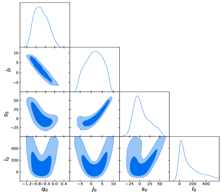
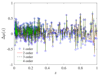
Using the JLA compilation, we obtain the cosmographic parameters up to the fourth order. We show the corresponding results in Figs. 1, 2, 3 and Table 1.

For the $z$-redshift, we can roughly distinguish the data and cosmographic models by residuals in Fig. 3. On the one hand, most of the data locate at the low redshift, and fit well with the models. On the other hand, some of the data at high redshift present a little bigger residual with the cosmographic models. Thus, more low-$z$ data make the cosmography study more precise. From the constraints in Table 1, we note that all of the constraints on parameter $q_{0}$ in $1\sigma$ confidence level are negative, which shows a recent accelerating expansion. However, some recent work try to find out a slowing down of the acceleration. Moreover, this novel phenomenon has attracted much attention Shafieloo et al. (2009); Cárdenas et al. (2013); Li et al. (2011); Lin et al. (2013); Magaña et al. (2014); Wang et al. (2016), including the recent work Magaña et al. (2017). Using the dark energy parameterizations, they found that the cosmic acceleration may has already peaked, and the expansion may be slowing down from the deceleration parameter $q_{0}>0$. In recent work Seikel et al. (2012); Zhang and Xia (2016), a model-independent analysis on this interesting subject was presented, using the powerful Gaussian processes technique. It was found that no slowing down is detected within $2\sigma$ C.L. from current data. Moreover, we analyzed the inconsistency in Ref.Zhang and Xia (2016). We further deduced what physical condition should be satisfied by the observational data Zhang and Xia (2017). These results are consistent with the cosmographic constraint from JLA data.

Figure 2: Constraints on cosmographic parameters in the 4 order from the JLA compilation for $y$-redshift.

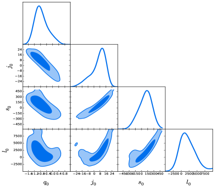
Comparison between Fig. 1 and 2 shows that degeneracies among the parameters in the $y$-redshift are similar as the $z$-redshift. The difference is that it provides much bigger errors on some parameters. Taking the parameter $l_{0}$ as an example, we find that its absolute value behaves an increasing trend. Moreover, its relative error in the $y$-redshift 2478.44/2056.97 is also bigger than that of the $z$-redshift 158.08/149.54. This is consistent with the result in previous work, namely, $y$-redshift brings worse constraints.

Figure 3: Residuals between the cosmographic distance modulus with different orders and the observational SNIa data. The vertical coordinates $\Delta\mu(z)=\mu^{\textmd{cos}}(z)-\mu^{\textmd{obs}}(z)$ denotes the residuals.

Table 1: Constrained cosmographic parameters by the JLA compilation and mock data within $1\sigma$ confidence level.

$\begin{array}[]{c c r@{ }l c r@{ }l c r@{ }l c r@{ }l}\hline\cr\hline\cr\hbox{\multirowsetup data}&\lx@intercol\hfil q_{0}\hfil\lx@intercol&\lx@intercol\hfil j_{0}\hfil\lx@intercol&\lx@intercol\hfil s_{0}\hfil\lx@intercol&\lx@intercol\hfil l_{0}\hfil\lx@intercol\\ &\lx@intercol\hfil\textmd{best fit}\hfil\lx@intercol&\lx@intercol\hfil\textmd{mean}\hfil\lx@intercol&\lx@intercol\hfil\textmd{best fit}\hfil\lx@intercol&\lx@intercol\hfil\textmd{mean}\hfil\lx@intercol&\lx@intercol\hfil\textmd{best fit}\hfil\lx@intercol&\lx@intercol\hfil\textmd{mean}\hfil\lx@intercol&\lx@intercol\hfil\textmd{best fit}\hfil\lx@intercol&\lx@intercol\hfil\textmd{mean}\hfil\lx@intercol\\ \hline\cr\lx@intercol\texttt{model}:z-\texttt{redshift}\hfil\lx@intercol\\ \textmd{JLA}&-0.46&-0.46&\pm 0.04&&&&&&&&&\\ &-0.45&-0.44&\pm 0.09&0.41&0.42&\pm 0.24&&&&&&\\ &-0.62&-0.50&\pm 0.09&1.93&1.06&\pm 0.56&1.77&0.50&\pm 1.15&&&\\ &-0.67&-0.58&\pm 0.29&2.54&1.45&\pm 3.82&3.98&4.97&\pm 20.35&19.90&149.54&\pm 158.08\\ \hline\cr\lx@intercol\texttt{model}:y-\texttt{redshift}\hfil\lx@intercol\\ \textmd{JLA}&-0.72&-0.71&\pm 0.07&&&&&&&&&\\ &-0.42&-0.45&\pm 0.20&-0.15&0.14&\pm 1.82&&&&&&\\ &-0.86&-0.88&\pm 0.44&7.71&8.64&\pm 7.92&81.72&114.83&\pm 113.52&&&\\ &-0.78&-0.74&\pm 0.45&6.36&6.16&\pm 10.06&69.69&89.06&\pm 160.80&851.04&2056.97&\pm 2478.44\\ \textmd{WFIRST}&&\sigma_{q_{0}}&=0.15&&\sigma_{j_{0}}&=4.11&&\sigma_{s_{0}}&=69.52&&\sigma_{l_{0}}&=1146.30\\ \textmd{redshift drift}&&\sigma_{q_{0}}&=0.51&&\sigma_{j_{0}}&=4.75&&\sigma_{s_{0}}&=242.11&&\sigma_{l_{0}}&=1299.17\\ \hline\cr\hline\cr\end{array}$

In recent years, many work focus on the question of which series truncation fits the data best. In previous work Cattoën and Visser (2008); Vitagliano et al. (2010); Xia et al. (2012), one introduced the F-test to find this answer, by favoring one model, and assessing the other alternative model. Although it showed that expansion up to the jerk term is a better description for observational luminosity distance, the cosmographic problem is still vague. It is difficult for us to escape from the maze of cosmography in the accuracy and precision. We should underline that small error does not mean a credible description, and big error is not necessarily a bad thing. For further analysis upon this issue, we recommend the bias-variance tradeoff Wasserman (2006)

risk $$= \textmd{bias}^{2}+\textmd{variance}$$ (25)

$$= \sum_{i=1}^{N}[\mu^{\textmd{cos}}(z_{i})-\tilde{\mu}(z_{i})]^{2}+\sum_{i=1}^{N}\sigma^{2}(\mu^{\textmd{cos}}(z_{i}))$$

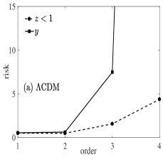
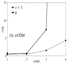
where $\mu^{\textmd{cos}}(z_{i})$ is the reconstructed cosmographic distance modulus in different series truncations, $\tilde{\mu}(z_{i})$ is the fiducial value, $\sigma(\mu^{\textmd{cos}}(z_{i}))$ is the uncertainty of reconstruction. Obviously, the bias-variance tradeoff can reveal more detailed information. The term bias² describes its accuracy (about the deviation from the true values), the variance conveys the precision (about the errors) of the constraint. Theoretically, minimizing risk corresponds to a balance between bias and variance. In cosmology, this promising approach has been widely utilized to find an effective way of obtaining information about the dark energy equation of state $w(z)$ Huterer and Starkman (2003); Zheng et al. (2014). In order to investigate the influence from fiducial model on the risk, we respectively consider the fiducial $\Lambda$CDM model with $\Omega_{m}=0.305$ and $w$CDM model with $w=-1.027$ in the combination of JLA and complementary probes Betoule et al. (2014).

IV.1.1 Accuracy

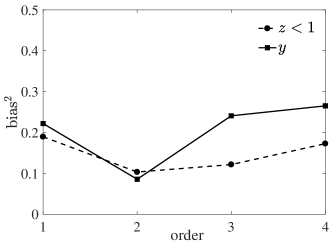
Accuracy is a deviation from the true value, which can be expressed by the bias square. In Fig. 4 we show the bias² of current data at the basis of fiducial $\Lambda$CDM model. First, we find that all of the bias are small, which indicates that the cosmographic models fit well with the JLA data. It implies that the cosmography is enough accurate to describe the observational JLA data. This is not difficult to understand, because about 99% of the JLA data are at low redshift. Thus, application of the JLA data in cosmology would be a very useful strategy. Second, we see that bias square slightly increases for higher order. Last but important, we obtain that the $z$-redshift and $y$-redshift both favor the 2 order, which indicates that expansion up to the jerk term is in the best agreement with the true values.

IV.1.2 Precision

Figure 4: Bias square in the $z$-redshift and $y$-redshift of the JLA compilation with different cosmographic series truncations at the basis of fiducial $\Lambda$CDM model.

Figure 5: Variance in the $z$-redshift and $y$-redshift of the JLA compilation with different cosmographic series truncations.

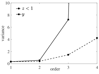
Precision is usually statistic, and represents the errors. Variance, the set of error, is independent of the fiducial model. In Fig. 5, we plot the variance of cosmographic model in $z$-redshift and $y$-redshift. First, variances at low order in these two redshift spaces are both small, almost zero. It indicates that current observational data can present a precise measurement on the parameters $q_{0}$ and $j_{0}$. Second, we note that variance at the 3 order starts to increase rapidly, especially for the $y$-redshift, which means that current data cannot give physical measurement on the $s_{0}$ term, even higher orders. However, it has enough information for us to infer that the universe will be to continue accelerate or slow down. Third, we should admit that variance in the $y$-redshift space at the 4 order is larger than that of the $z$-redshift.

IV.1.3 Risk

Risk is used to balance the bias square and variance, and to find which series truncation is the best description of the observational data. Due to the model-dependence of bias square, in this section we also investigate the influence of different fiducial models on the final risk analysis. In Fig. 6, we plot the risk for fiducial $\Lambda$CDM model and $w$CDM model. From the comparison between two panels, we first find that risk affected by the fiducial model is so little. They both favor that cosmography up to the $j_{0}$ term is a better choice to describe current JLA data. This consequence is consistent with our previous work via the F-test Xia et al. (2012). It also proves that the risk analysis is a stable and scientific tool to analyze the convergence problem.

From the bias-variance tradeoff, we conclude that the JLA data is so precise that the cosmographic model at $z$-redshift and $y$-redshift both can present an estimation with high accuracy. Of course, the introduction of $y$-redshift can improve the cosmography study to higher redshift region, even to the early epoch. With its help, past universe can be understood more objective. Meanwhile, the risk analysis is also stable. Effect by the redshift parameter and fiducial model is not significant.

Figure 6: Risk with different cosmographic series truncations in diverse fiducial models. The panel (a) is for the $\Lambda$CDM model, and the panel (b) is for $w$CDM model.

Figure 7: Variance for different cosmographic series truncations in the $y$-redshift by current and future observations.

IV.2 Forecasting

Figure 8: Cosmographic distance modulus, Hubble parameter and deceleration parameter with different orders in the $y$-redshift.

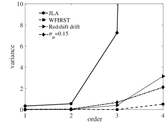
Above analysis shows that cosmography at high order suffers unphysical estimation, i.e., large variance. We anticipate that future observation is able to give tighter constraints on the cosmography, with the improvement of observational precision, thus leading to a relaxation of the convergence problem. In this section, we forecast the constraint from future WFIRST and redshift drift on cosmography. In order to test the constraint from mock distance modulus with flat errors $\sigma_{\mu}=0.15$, we also generate some data following the work in Ref. Busti et al. (2015). Comparison in Table 1 shows that future measurement can improve the constraints. For example, compared with $\sigma_{l_{0}}=2478.44$ from the JLA sample, the redshift drift gives a more robust constraint on the parameters, e.g., $\sigma_{l_{0}}=1299.17$, almost improving by double than current JLA data. Due to future measurements mainly focus on the high redshift region, we make a comparison on variance for the $y$-redshift in Fig. 7. On the one hand, we find that all the future observations can improve the constraints at low order with high significant. Especially, the redshift drift can present an error $\sigma_{q_{0}}\sim 10^{-5}$ for the 1 order. On the other hand, the future observations, including the mock data with $\sigma_{\mu}=0.15$ all improve the constraint at high order dramatically. Variances in these cases are much smaller than current data. Thus, we can see that the bias-trade off is effective to estimate the cosmographic problem. The future observations also have the potential to solve the cosmographic problem.

V Values of the cosmography

Figure 9: Cosmographic EoS for different orders with matter density $\Omega_{m}=$0.25, 0.30 and 0.35, respectively.

Figure 10: Derivative of dark energy EoS $\textmd{d}w/\textmd{d}z$ for different cosmographic orders with varying parameter $\Omega_{m}$ from 0.25 to 0.35.

In previous work, cosmography has been widely used to reconstruct some special cosmological parameters, because of its model-independence. In this section, we are interested in investigating its values to report what information we can obtain from the cosmography, and what we cannot get.

V.1 Deceleration parameter

Deceleration parameter is important for its sharp sense on the cosmic expansion. Especially, its negative (positive) sign immediately indicates the accelerating (decelerating) expansion. However, it is not an observable quantity temporarily. Most studies were performed in multiform parameterized $q(z)$. Therefore, a model-independent analysis is appreciated.

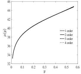
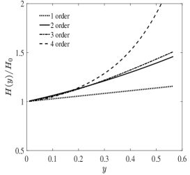
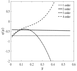
In the right panel of Fig. 8, we plot the reconstructed deceleration factor over $y$-redshift using the best-fit values of supernova data. We find that $q(y)$ in various series truncations are quite different. It strongly depends on the order of Taylor expansion. Therefore, it is difficult to obtain a model-independent and stable estimation on the deceleration parameter via cosmography.

In order to find the reason why we cannot obtain a stable estimation on deceleration parameter, we also compare the cosmographic distance modulus and Hubble parameter for different orders. For the distance modulus, they are almost indistinguishable at all redshift, which indicates that cosmography fit well with the observational data. However, for the Hubble parameter, we can only obtain a relatively stable estimation at low redshift $y<0.2$. For high redshift, they gradually deviate from each other. When we extract the information of deceleration parameter, we only can obtain a similar estimation at redshift $y\approx 0.1$. This comparison tells us that despite the cosmographic models fit well with the data, their contradiction become more and more prominent, with our increasing requirement on cosmic expansion study. Therefore, it is difficult to obtain a more detailed expansion history via cosmography.

In fact, Fig. 8 implies that a dynamical measurement may be useful to solve this contradiction. In our previous work Xia et al. (2012), we found that inclusion of Hubble parameter data can lead to stronger constraints on cosmographic parameters. In Ref. Neben and Turner (2013), the authors also showed that the distance indicator cannot directly measure $q_{0}$ with both accuracy and precision. However, the redshift drift may be possible to do it. Therefore, it is reasonable for us to anticipate that inclusion of the dynamical redshift drift could present a much more stable evaluation on cosmic expansion history.

V.2 Dark energy equation of state

In previous work, cosmography was often used to reconstruct the dynamical cosmological model. For example, with two cosmographic parameters $(q_{0},j_{0})$, one can derive the constant equation of state (EoS) dark energy model Demianski et al. (2012)

$$\Omega_{m}(q_{0},j_{0}) = \frac{2(j_{0}-q_{0}-2q_{0}^{2})}{1+2j_{0}-6q_{0}},$$

$$w_{0}(q_{0},j_{0}) = \frac{1+2j_{0}-6q_{0}}{-3+6q_{0}}.$$ (26)

However, it needs a background model. In order to get an undamaged map of dark energy, our study is in the normal cosmological model

$$H^{2}(z)=H_{0}^{2}\left[\Omega_{m}(1+z)^{3}+(1-\Omega_{m})\exp\Big{[}3\int_{0}^{z}\frac{1+w(z)}{1+z}\Big{]}dz\right].$$ (27)

In our analysis, we do not impose any style of dark energy, but the common $w(z)$. Solving the Eq. (27), we obtain

$$1+w(z)=\frac{1}{3}\frac{[H^{2}(z)-H^{2}_{0}\Omega_{m}(1+z)^{3}]^{\prime}(1+z)}{H^{2}(z)-H^{2}_{0}\Omega_{m}(1+z)^{3}},$$ (28)

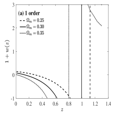
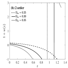
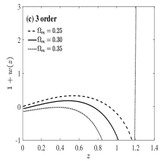
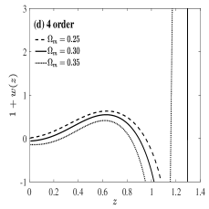
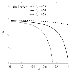
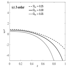
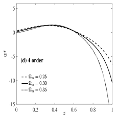
where the prime denotes the derivative with respect to redshift $z$. For the Eq. (28), we note that the denominator may be zero for $H(z)^{2}=H_{0}^{2}\Omega_{m}(1+z)^{3}$. This case may leads to a singularity in the EoS reconstruction. In Fig. 9, we plot the reconstruction of dark energy with different cosmographic series. In order to investigate the influence of matter density parameter, we relax parameter $\Omega_{m}$ from 0.25 to 0.35. On the one hand, we find that cosmography all favor a cosmological constant EoS at recently. On the other hand, however, a reliable estimation on $w(z)$ is difficult to obtain. In addition, we find that $w(z)$ at redshift $z\sim 0.8$ has a sharp change, independent of the matter density parameter.

Usually, it is difficult to determine the EoS constant or varying model independently. A model-independent analysis of the derivative of EoS can be studied using the cosmography

$$w^{\prime}=\frac{\textmd{d}w}{\textmd{d}z}.$$ (29)

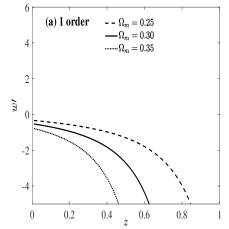
In Fig. 10, we plot the derivative $w^{\prime}(z)$ by cosmography with different series. We also consider the parameter $\Omega_{m}$ in a wide region. At first, we find that $w^{\prime}(z=0)$ is not zero in different cosmographic models. This indicates that a constant EoS dark energy model may be inappropriate. Moreover, $w^{\prime}(z)$ at low redshift are generally negative. Thus, the cosmography may suggest a varying EoS and more complicated dark energy candidate. Linear EoS like $w(z)=w_{0}+w_{a}z$ may be improper. According to above picture, we infer that cosmography may favor a dark energy with $w(z)=-1+w_{a}z+w_{b}z^{2}+\cdots$, where $w_{a}<0$ and $w_{b}\neq 0$. However, an accurate determination on the derivative $w^{\prime}(z)$ need more data to join in, because it also strongly depends on the cosmographic series truncation.

VI Conclusion and discussion

In the present paper, we analyse the problem of cosmography using the bias-variance tradeoff, and investigate its values.

To solve the convergence issue in cosmography, an improved redshift $y=z/(1+z)$ was introduced. Using the bias-variance tradeoff, we find that the $y$-redshift produces bigger variances at high orders. For the low cosmographic order (i.e., 1 order and 2 order), $y$-redshift does not bring bigger errors, but a nearly identical variance as $z$-redshift. For the JLA data, we find that most of them distribute in low redshift region with high precision. So that, the $z$-redshift is enough accurate to describe the data. Although the $y$-redshift does not present a smaller bias than $z$-redshift for the JLA data, it still can ensure the correctness of cosmography at high redshift.

Minimizing risk, it suggests that expansion up to the $j_{0}$ term is the best choice for current supernova data, regardless of the $z$-redshift or $y$-redshift. We also test the influence of fiducial model on risk analysis. The comparison demonstrates that it is trivial. Although previous F-test also obtained a similar result, our paper is not a repeated work using more data. Our analysis finds out deeper reason of the convergence issue. First, it not only can tell us the convergence problem is in the accuracy or the precision, but also can provide us more objective information about how serious the divergence problem is. Because if the crux lies on the accuracy, the convergence problem maybe still cannot be solved even thought more data were included. Second, in previous work, most focus were on the pursuit of “sweet spot”, which has masked the physical meaning of $y$-redshift. In our study, we not only find it is influenced by the distribution of data, but also forecast whether future observations can solve the convergence problem. Our analysis in Fig. 8 and Section V.1 also indicates that the dynamical measurement is a potential clue to solve this problem.

Our forecast finds that future WFIRST and redshift drift can significantly improve the constraints. Therefore, inclusion of dynamical measurement such as Hubble parameter data, redshift drift, etc. may be able to improve the constraint in accuracy and precision with high significance. As studied in our previous work Xia et al. (2012), inclusion of the $H(z)$ data can lead to stronger constraints on the cosmographic parameters. This discovery is helpful to understand or solve the convergence issue of supernova data. This is because dynamical probe like the canonical redshift drift can provide direct measurement to the cosmic expansion history. While distance measurement is geometric. As studied in Ref. Maor et al. (2001), the luminosity distance determines the EoS $w$ through a multiple integral relation that smears out much information. For the redshift drift, it not only directly measures the change of Hubble parameter, but also can be realized via multiple wavebands and methods Loeb (1998); Darling (2012). Moreover, it is immune from extra systematic errors, and does not need photometric calibration etc. Recently, a test in German Vacuum Tower Telescope demonstrates that the Laser Frequency Combs also have an advantage with long-term calibration precision, accuracy to realize the redshift drift experiment Steinmetz et al. (2008).

Our investigation also promotes the study of the values of cosmography. In previous work, most attention were focus on a special model. However, our analysis presents a almost undamaged map of dark energy. It breaks the limitation of extrapolation to other models. Setting the dark energy $w(z)$ as free, we find that cosmography cannot give reliable estimations on $q(z)$ and $w(z)$. However, we find that it does not favor a constant EoS, but a complicated $w(z)$, such as $w(z)=-1+w_{a}z+w_{b}z^{2}+\cdots$, where $w_{a}<0$ and $w_{b}\neq 0$. These estimations are useful for modelling the dark energy.

Cosmography has been an useful tool with great potential to study the cosmology. For the dark energy, it was usually reconstructed by parametrization, such as the Chevallier-Polarski-Linder Chevallier and Polarski (2001); Linder (2003), Jassal-Bagla-Padmanabhan Jassal et al. (2005); or the non-parameterization, such as the Gaussian processes Seikel et al. (2012); Nair et al. (2014), principal component analysis Crittenden et al. (2012); Zheng et al. (2014). Cosmography is another model-independent method to assess dark energy models. Moreover, cosmography has also been widely used in another fields, such as to test the power of supernova data Ma and Corasaniti (2016). Therefore, we have to say that cosmography is an important method to study the cosmology. Our study provides a straightforward and scientific reference. Of course, we will also devote ourselves to improving the cosmography study in our future work. We would like to study the influence of the inclusion of BAO and CMB data on cosmography. Throughout previous work, we find that many different observational data or combinations favor the best cosmography with 2 order. In our future work, we are also interested in exploring their subtle relations to further understand the cosmography. Moreover, we also has an interest to improve the cosmographic problem by proposing some other physical redshift.

References

- Carroll et al. (1992) S. M. Carroll, W. H. Press, and E. L. Turner, Annu. Rev. Astron. Astrophys. 30, 499 (1992).
- Caldwell et al. (2003) R. R. Caldwell, M. Kamionkowski, and N. N. Weinberg, Phys. Rev. Lett. 91, 071301 (2003).
- Feng et al. (2005) B. Feng, X. Wang, and X. Zhang, Phys. Lett., B 607, 35 (2005).
- Barrow and Cotsakis (1988) J. D. Barrow and S. Cotsakis, Phys. Lett. B 214, 515 (1988).
- Dvali et al. (2000) G. Dvali, G. Gabadadze, and M. Porrati, Phys. Lett. B 485, 208 (2000).
- Lemaître (1933) G. Lemaître, Annales de la Societe Scietifique de Bruxelles 53, 51 (1933).
- Tolman (1934) R. C. Tolman, Proceedings of the national academy of sciences of the United States of America 20, 169 (1934).
- Bondi (1947) H. Bondi, Mon. Not. R. Astron. Soc. 107, 410 (1947).
- Chiba and Nakamura (1998) T. Chiba and T. Nakamura, Progress of theoretical physics 100, 1077 (1998).
- Visser (2004) M. Visser, Classical and Quantum Gravity 21, 2603 (2004).
- Cattoën and Visser (2007) C. Cattoën and M. Visser, Classical and Quantum Gravity 24, 5985 (2007).
- Aviles et al. (2012) A. Aviles, C. Gruber, O. Luongo, and H. Quevedo, Physical Review D 86, 123516 (2012).
- Cattoën and Visser (2008) C. Cattoën and M. Visser, Phys. Rev. D 78, 063501 (2008).
- Capozziello et al. (2011) S. Capozziello, R. Lazkoz, and V. Salzano, Physical Review D 84, 124061 (2011).
- Xia et al. (2012) J.-Q. Xia, V. Vitagliano, S. Liberati, and M. Viel, Phys. Rev. D 85, 043520 (2012).
- Vitagliano et al. (2010) V. Vitagliano, J.-Q. Xia, S. Liberati, and M. Viel, Journal of Cosmology and Astroparticle Physics 2010, 005 (2010).
- Lazkoz et al. (2013) R. Lazkoz, J. Alcaniz, C. Escamilla-Rivera, V. Salzano, and I. Sendra, Journal of Cosmology and Astroparticle Physics 12, 005 (2013).
- Busti et al. (2015) V. C. Busti, Á. de la Cruz-Dombriz, P. K. S. Dunsby, and D. Sáez-Gómez, Physical Review D 92, 123512 (2015).
- Suzuki et al. (2012) N. Suzuki, D. Rubin, C. Lidman, et al., Astrophys. J. 746, 85 (2012).
- Sandage (1962) A. Sandage, Astrophys. J. 136, 319 (1962).
- Liske et al. (2008a) J. Liske, A. Grazian, E. Vanzella, et al., Mon. Not. R. Astron. Soc. 386, 1192 (2008a).
- Liske et al. (2008b) J. Liske, A. Grazian, E. Vanzella, et al., The Messenger 133, 10 (2008b).
- Corasaniti et al. (2007) P.-S. Corasaniti, D. Huterer, and A. Melchiorri, Physical Review D 75, 062001 (2007).
- Zhang and Liu (2014) M.-J. Zhang and W.-B. Liu, The European Physical Journal C 74, 1 (2014).
- Geng et al. (2015) J.-J. Geng, Y.-H. Li, J.-F. Zhang, and X. Zhang, The European Physical Journal C 75, 1 (2015).
- Li et al. (2013) Z. Li, K. Liao, P. Wu, H. Yu, and Z.-H. Zhu, Phys. Rev. D 88, 023003 (2013).
- Uzan et al. (2008) J.-P. Uzan, C. Clarkson, and G. F. R. Ellis, Physical Review Letters 100, 191303 (2008).
- Yu et al. (2014) H.-R. Yu, T.-J. Zhang, and U.-L. Pen, Physical Review Letters 113, 041303 (2014).
- Sahni et al. (2003) V. Sahni, T. D. Saini, A. A. Starobinsky, and U. Alam, Journal of Experimental and Theoretical Physics Letters 77, 201 (2003).
- Alam et al. (2003) U. Alam, V. Sahni, T. D. Saini, and A. Starobinsky, Monthly Notices of the Royal Astronomical Society 344, 1057 (2003).
- Jimenez and Loeb (2008) R. Jimenez and A. Loeb, The Astrophysical Journal 573, 37 (2008).
- Simon et al. (2005) J. Simon, L. Verde, and R. Jimenez, Phys. Rev. D 71, 123001 (2005).
- Stern et al. (2010) D. Stern, R. Jimenez, L. Verde, M. Kamionkowski, and S. A. Stanford, Journal of Cosmology and Astroparticle Physics 2010, 008 (2010).
- Gaztanaga et al. (2009) E. Gaztanaga, A. Cabre, and L. Hui, Monthly Notices of the Royal Astronomical Society 399, 1663 (2009).
- Moresco et al. (2012) M. Moresco, A. Cimatti, R. Jimenez, et al., Journal of Cosmology and Astroparticle Physics 08, 006 (2012).
- Busca et al. (2013) N. G. Busca, T. Delubac, J. Rich, et al., Astronomy and Astrophysics 552, A96 (2013), eprint 1211.2616.
- Loeb (1998) A. Loeb, Astrophys. J. Letters 499, L111 (1998).
- Martinelli et al. (2012) M. Martinelli, S. Pandolfi, C. J. A. P. Martins, and P. E. Vielzeuf, Phys. Rev. D 86, 123001 (2012).
- Moraes and Polarski (2011) B. Moraes and D. Polarski, Phys. Rev. D 84, 104003 (2011).
- Zhang et al. (2014) M.-J. Zhang, J.-Z. Qi, and W.-B. Liu, International Journal of Theoretical Physics 54, 2456 (2014).
- Balcerzak and Dabrowski (2014) A. Balcerzak and M. P. Dabrowski, Physics Letters B 728, 15 (2014).
- Lewis and Bridle (2002) A. Lewis and S. Bridle, Physical Review D 66, 103511 (2002).
- Betoule et al. (2014) M. Betoule, R. Kessler, J. Guy, et al., Astronomy & Astrophysics 568, A22 (2014).
- Bochner et al. (2015) B. Bochner, D. Pappas, and M. Dong, The Astrophysical Journal 814, 7 (2015), eprint 1308.6050.
- Spergel et al. (2015) D. Spergel, N. Gehrels, C. Baltay, D. Bennett, J. Breckinridge, M. Donahue, A. Dressler, B. Gaudi, T. Greene, O. Guyon, et al., arXiv:1503.03757 (2015).
- Pasquini et al. (2006) L. Pasquini, S. Cristiani, H. Dekker, et al., Scientific Requirements for Extremely Large Telescopes 232, 193 (2006).
- Pasquini et al. (2005) L. Pasquini, S. Cristiani, H. Dekker, et al., The Messenger 122, 10 (2005).
- Shafieloo et al. (2009) A. Shafieloo, V. Sahni, and A. A. Starobinsky, Phys. Rev. D 80, 101301 (2009).
- Cárdenas et al. (2013) V. H. Cárdenas, C. Bernal, and A. Bonilla, Mon. Not. R. Astron. Soc. 433, 3534 (2013).
- Li et al. (2011) Z. Li, P. Wu, and H. Yu, Phys. Lett. B 695, 1 (2011).
- Lin et al. (2013) J. Lin, P. Wu, and H. Yu, Phys. Rev. D 87, 043502 (2013).
- Magaña et al. (2014) J. Magaña, V. H. Cárdenas, and V. Motta, Journal of Cosmology and Astroparticle Physics 10, 017 (2014).
- Wang et al. (2016) S. Wang, Y. Hu, M. Li, and N. Li, Astrophys. J. 821, 60 (2016), eprint 1509.03461.
- Magaña et al. (2017) J. Magaña, V. Motta, V. H. Cárdenas, and G. Foëx, Mon. Not. R. Astron. Soc. 469, 47 (2017), eprint 1703.08521.
- Seikel et al. (2012) M. Seikel, C. Clarkson, and M. Smith, Journal of Cosmology and Astroparticle Physics 2012, 036 (2012).
- Zhang and Xia (2016) M.-J. Zhang and J.-Q. Xia, Journal of Cosmology and Astroparticle Physics 12, 005 (2016).
- Zhang and Xia (2017) M.-J. Zhang and J.-Q. Xia, arXiv:1701.04973 (2017).
- Wasserman (2006) L. Wasserman, All of Nonparametric Statistics (Springer Science & Business Media, 2006).
- Huterer and Starkman (2003) D. Huterer and G. Starkman, Phys. Rev. Lett. 90, 031301 (2003).
- Zheng et al. (2014) W. Zheng, S.-Y. Li, H. Li, J.-Q. Xia, M. Li, and T. Lu, Journal of Cosmology and Astroparticle Physics 2014, 030 (2014).
- Neben and Turner (2013) A. R. Neben and M. S. Turner, Astrophys. J. 769, 133 (2013).
- Demianski et al. (2012) M. Demianski, E. Piedipalumbo, C. Rubano, and P. Scudellaro, Monthly Notices of the Royal Astronomical Society 426, 1396 (2012).
- Maor et al. (2001) I. Maor, R. Brustein, and P. J. Steinhardt, Physical Review Letters 86, 6 (2001).
- Darling (2012) J. Darling, Astrophys. J. Letters 761, L26 (2012).
- Steinmetz et al. (2008) T. Steinmetz, T. Wilken, C. Araujo-Hauck, R. Holzwarth, T. W. Hänsch, L. Pasquini, A. Manescau, S. D’Odorico, M. T. Murphy, T. Kentischer, et al., Science 321, 1335 (2008).
- Chevallier and Polarski (2001) M. Chevallier and D. Polarski, International Journal of Modern Physics D 10, 213 (2001).
- Linder (2003) E. V. Linder, Physical Review Letters 90, 091301 (2003).
- Jassal et al. (2005) H. K. Jassal, J. S. Bagla, and T. Padmanabhan, Mon. Not. R. Astron. Soc. 356, L11 (2005), eprint astro-ph/0404378.
- Nair et al. (2014) R. Nair, S. Jhingan, and D. Jain, Journal of Cosmology and Astro-Particle Physics 1, 005 (2014).
- Crittenden et al. (2012) R. G. Crittenden, G.-B. Zhao, L. Pogosian, L. Samushia, and X. Zhang, Journal of Cosmology and Astroparticle Physics 2012, 048 (2012).
- Ma and Corasaniti (2016) C. Ma and P.-S. Corasaniti, arXiv:1604.04631 (2016).