Diffusive Boltzmann equation, its fluid dynamics, Couette flow and Knudsen layers

Abstract.

In the current work we construct a multimolecule random process which leads to the Boltzmann equation in the appropriate limit, and which is different from the deterministic real gas dynamics process. We approximate the statistical difference between the two processes via a suitable diffusion process, which is obtained in the multiscale homogenization limit. The resulting Boltzmann equation acquires a new spatially diffusive term, which subsequently manifests in the corresponding fluid dynamics equations. We test the Navier-Stokes and Grad closures of the diffusive fluid dynamics equations in the numerical experiments with the Couette flow for argon and nitrogen, and compare the results with the corresponding Direct Simulation Monte Carlo (DSMC) computations. We discover that the full-fledged Knudsen velocity boundary layers develop with all tested closures when the viscosity and diffusivity are appropriately scaled in the vicinity of the walls. Additionally, we find that the component of the heat flux parallel to the direction of the flow is comparable in magnitude to its transversal component near the walls, and that the nonequilibrium Grad closure approximates this parallel heat flux with good accuracy.

1. Introduction

In the kinetic theory, the processes in gases are described by the Boltzmann equation [9, 10, 11, 12], which models the evolution of the density $f(t,\boldsymbol{x},\boldsymbol{v})$ of a probability distribution of a single gas molecule in the space of coordinate $\boldsymbol{x}$ and velocity $\boldsymbol{v}$ at time $t$, under the assumption that all gas molecules are independently and identically distributed, and that no more than two molecules collide at once. The Boltzmann equation is given by

(1.1) $$\frac{\partial f}{\partial t}+\boldsymbol{v}\cdot\nabla_{\boldsymbol{x}}f=\mathcal{C}(f),$$

where $\mathcal{C}(f)$ is the collision term (also called the collision operator [33, 21]), specified by

(1.2) $$\mathcal{C}(f)=\int B(|(\boldsymbol{w}-\boldsymbol{v})\cdot\boldsymbol{n}|)\big{(}f(\boldsymbol{v}^{\prime})f(\boldsymbol{w}^{\prime})-f(\boldsymbol{v})f(\boldsymbol{w})\big{)}\,\mathrm{d}\boldsymbol{n}\,\mathrm{d}\boldsymbol{w}.$$

Above, $\boldsymbol{n}$ is a unit vector, the integration in $\,\mathrm{d}\boldsymbol{n}$ is over a unit sphere, $B$ is the collision kernel, and $\boldsymbol{v}^{\prime}$, $\boldsymbol{w}^{\prime}$ are defined by the energy and momentum conservation relations

(1.3) $$\boldsymbol{v}^{\prime}=\boldsymbol{v}+((\boldsymbol{w}-\boldsymbol{v})\cdot\boldsymbol{n})\boldsymbol{n},\qquad\boldsymbol{w}^{\prime}=\boldsymbol{w}+((\boldsymbol{v}-\boldsymbol{w})\cdot\boldsymbol{n})\boldsymbol{n}.$$

Integrating the Boltzmann equation over various powers of the velocity variable yields the hierarchy of the fluid dynamics equations (also called the moment equations in kinetic theory), of which the lowest-order closure is provided by the well known Euler equations [3], while the next-order closure is given by the Grad equations [22, 23].

The Boltzmann equation and its corresponding hierarchy of the moment fluid dynamics equations are of the first order in space, which makes them poorly suitable for boundary value problems. However, various formulations of boundary conditions are rather ubiquitous in the applied problems for realistic flows (for example, the Couette and Poiseuille flows). For the fluid dynamics equations, the second order in space is usually achieved via the Chapman-Enskog perturbation expansion [13, 21, 33], which, when applied to the Euler closure, leads to the famous Navier-Stokes equations [3], for which boundary value problems are usually well posed.

Recently, there appeared a number of works on the extended Boltzmann equation and the corresponding fluid dynamics [6, 7, 8, 15, 18, 16, 29, 38], where a spatial diffusion term was introduced in addition to the collision operator or viscous terms. Some of these works [6, 7, 8] were based on the idea of introducing the concept of the “volume velocity”, which differs from the usual mass velocity by a small flux term derived from Fick’s law. Others [18, 16] introduced similar additional terms to model the self-diffusion of mass. Among those listed above, the works [15, 29, 38] appear to employ the closest conceptual approach to what we suggest here, namely, in [15, 29, 38] an ad hoc diffusion term was introduced directly into the Boltzmann equation (1.1) via the assumption of an additional empirical stochasticity of the molecular motion to complement the already present inter-molecule collisions. However, the main conceptual drawback of such an approach is its seeming absence of a fundamental justification. In particular, it was noted in [15] that there did not seem to be a thermodynamically valid reason to introduce an additional diffusion term into a continuum gas model.

In the current work, we identify the difference between the actual dynamics of a real gas, and the dynamics which are described by the Boltzmann equation in (1.1). More specifically, we construct the precise multimolecular dynamical system which leads directly to the Boltzmann equation in the appropriate limit, and this system turns out to be fundamentally different from the realistic gas dynamics. While the real gas dynamics is fully deterministic with the molecular trajectories prescribed exactly via the initial conditions, the multimolecular system we introduce is a random jump process (more precisely, a Lévy-type Feller process [2]), whose stochasticity is inherent. Then, we approximate the difference between the two dynamics via a multscale formalism in the homogenization time limit [27, 28, 36, 44, 45], which equips the Boltzmann equation and the corresponding fluid dynamics equations with an additional spatially diffusive term.

The manuscript is organized as follows. In Section 2 we consider the multimolecular motion of a realistic gas where the intermolecular interactions are governed by a repelling potential, and arrive at the conclusion that the deterministic multimolecular Liouville equation cannot be directly simplified into the Boltzmann equation without an appropriate stochastic modification. In Section 3 we construct the aforementioned multimolecular random jump process, whose Kolmogorov equation naturally reduces to the Boltzmann equation in the appropriate limit. In Section 4 we approximate the difference between the two multimolecular systems in the multiscale homogenization time limit, which leads to an Itô diffusion process. In Section 5 we augment the multimolecular random jump process with the corrective Itô diffusion process, such that the resulting Boltzmann equation acquires a spatial diffusion term, which corresponds to the diffusion of mass. In Section 6 we derive the diffusive Euler, Navier-Stokes, Grad [22, 23] and regularized Grad [39, 40, 42] equations, which also inherit the spatial diffusion terms. In Section 7 we carry out the numerical simulations for argon and nitrogen in the simple Couette flow setting, and compare them against the DSMC computations [4, 37]. We discover that if the viscosity and diffusivity are appropriately scaled in the vicinity of the walls [1], then all studied moment closures develop the full-fledged Knudsen velocity boundary layers in agreement with the DSMC computations. We also find that the diffusive Navier-Stokes equations produce a better temperature prediction than the conventional Navier-Stokes equations. We observe that the DSMC computations produce a substantial component of the heat flux parallel to the direction of the flow, which the Fourier law approximation of the Navier-Stokes equations fails to capture. On the other hand, both the diffusive and regularized diffusive Grad closures approximate the parallel heat flux, the latter with particularly good accuracy. The summary is given in Section 8.

2. The microscopic dynamics of a realistic gas

Here we consider a system of $K$ identical gas molecules, which move in an $N$-dimensional Euclidean space. For a realistic gas, the components $i=1,2,3$ of the space are translational, while $i=4,\ldots,N$ are rotational, and thus naturally periodic. Also, the way real gas molecules interact depends differently on the translational and rotational coordinates; clearly, the translational coordinates of a pair of molecules have to be similar for them to interact, while the alignment of their rotational coordinates weakly affect the occurrence or non-occurrence of a collision (but not its outcome, obviously).

For convenience, below we will treat all coordinates equivalently, as both translational, as far as the molecular interaction is concerned, and rotational, as we assume that the full coordinate space is Euclidean and periodic in each coordinate. In this sense, any gas we consider below is, in a way, “monatomic”, except that its phase space can be more than three-dimensional. While such an approach does not rigorously address the issues of collision between polyatomic gas molecules, below we will show that it is not needed for our purposes – we will fully decouple the rotational coordinates from the macroscopic equations of the gas dynamics. Besides, the collision of polyatomic molecules is a separate and rather complex subject in itself, and often phenomenological models (such as the Borgnakke-Larsen collision model [5]) are used to describe such collisions in practice.

In order to define a multimolecular dynamical system in a concise manner, we concatenate all coordinates $\boldsymbol{x}_{i}$ and velocities $\boldsymbol{v}_{i}$ of the individual molecules into the two vectors $\boldsymbol{X}$ and $\boldsymbol{V}$ as follows:

$$\boldsymbol{X}=\left(\boldsymbol{x}_{1},\boldsymbol{x}_{2},\ldots,\boldsymbol{x}_{K}\right),\qquad\boldsymbol{V}=\left(\boldsymbol{v}_{1},\boldsymbol{v}_{2},\ldots,\boldsymbol{v}_{K}\right).$$

Apparently, $\boldsymbol{X}$ and $\boldsymbol{V}$ have the dimension $KN$, since each $\boldsymbol{x}_{i}$ or $\boldsymbol{v}_{i}$ is $N$-dimensional.

We assume that the molecules interact with each other via a potential function $H(\boldsymbol{X})$, so that the equations of motion for the realistic gas molecules are given by

(2.1) $$\frac{\,\mathrm{d}\boldsymbol{X}}{\,\mathrm{d}t}=\boldsymbol{V},\qquad\frac{\,\mathrm{d}\boldsymbol{V}}{\,\mathrm{d}t}=-\nabla_{\boldsymbol{X}}H(\boldsymbol{X}).$$

In what follows, we will assume that the potential $H$ has the form of the sum of pairwise interactions between all molecules in the system:

(2.2) $$H(\boldsymbol{X})=\sum_{\genfrac{}{}{0.0pt}{}{i=1\ldots K-1}{j=i+1\ldots K}}\phi(\|\boldsymbol{x}_{i}-\boldsymbol{x}_{j}\|),$$

where $\phi(\|\boldsymbol{x}\|)$ is the potential of an individual molecule (for example, the Lennard-Jones potential [32]). It is easy to see that such a choice of $H$ ensures the conservation of the total momentum $\boldsymbol{m}$ and energy $E$ of the system,

(2.3) $$\boldsymbol{m}=\sum_{i=1\ldots K}\boldsymbol{v}_{i},\qquad E=\frac{1}{2}\|\boldsymbol{V}\|^{2}+H(\boldsymbol{X}).$$

Let $F(t,\boldsymbol{X},\boldsymbol{V})$ be the density distribution function of $\boldsymbol{X}$ and $\boldsymbol{V}$. Then, the evolution equation for $F$ is given by the corresponding Liouville equation (which is also the special case of the forward Kolmogorov equation [20] for a deterministic system) for the real gas:

(2.4) $$\frac{\partial F}{\partial t}+\boldsymbol{V}\cdot\nabla_{\boldsymbol{X}}F=\nabla_{\boldsymbol{X}}H\cdot\nabla_{\boldsymbol{V}}F.$$

The Liouville equation in (2.4) admits a special class of solutions in the form of the product of identical probability densities $f$ for each molecule,

(2.5) $$F(t,\boldsymbol{X},\boldsymbol{V})=\prod_{i=1\ldots K}f(t,\boldsymbol{x}_{i},\boldsymbol{v}_{i}).$$

Indeed, substituting (2.5) into (2.4), we obtain, for the different terms of (2.4),

(2.6a) $$\frac{\partial F}{\partial t}=\sum_{i=1}^{K}\left(\prod_{j\neq i}f(t,\boldsymbol{x}_{j},\boldsymbol{v}_{j})\right)\frac{\partial}{\partial t}f(t,\boldsymbol{x}_{i},\boldsymbol{v}_{i}),$$

(2.6b) $$\boldsymbol{V}\cdot\nabla_{\boldsymbol{X}}F=\sum_{i=1}^{K}\left(\prod_{j\neq i}f(t,\boldsymbol{x}_{j},\boldsymbol{v}_{j})\right)\boldsymbol{v}_{i}\cdot\nabla_{\boldsymbol{x}}f(t,\boldsymbol{x}_{i},\boldsymbol{v}_{i}),$$

(2.6c) $$\nabla H(\boldsymbol{X})\cdot\nabla_{\boldsymbol{V}}F=\sum_{i=1}^{K}\sum_{j\neq i}\bigg{(}\prod_{\genfrac{}{}{0.0pt}{}{k\neq i}{k\neq j}}f(t,\boldsymbol{x}_{k},\boldsymbol{v}_{k})\bigg{)}f(t,\boldsymbol{x}_{j},\boldsymbol{v}_{j})\nabla_{\boldsymbol{x}_{i}}\phi(\|\boldsymbol{x}_{i}-\boldsymbol{x}_{j}\|)\cdot\nabla_{\boldsymbol{v}}f(t,\boldsymbol{x}_{i},\boldsymbol{v}_{i}).$$

Substituting (2.6) into (2.4) and integrating over $\boldsymbol{x}_{i}$, $\boldsymbol{v}_{i}$, $i>1$, under the assumption that all $\boldsymbol{x}_{i}$- and $\boldsymbol{v}_{i}$-derivatives integrate out to zero we arrive at an equation for the distribution $f(t,\boldsymbol{x},\boldsymbol{v})$ of a single molecule in the closed form, known as the Vlasov equation:

(2.7) $$\frac{\partial f}{\partial t}+\boldsymbol{v}\cdot\nabla_{\boldsymbol{x}}f=\nabla_{\boldsymbol{x}}h\cdot\nabla_{\boldsymbol{v}}f,$$

where $h(\boldsymbol{x})$ is the combined potential of the remaining $(K-1)$ identical molecules:

(2.8) $$h(\boldsymbol{x})=(K-1)\int\phi(\|\boldsymbol{x}-\boldsymbol{y}\|)f(\boldsymbol{y},\boldsymbol{w})\,\mathrm{d}\boldsymbol{y}\,\mathrm{d}\boldsymbol{w}.$$

Thus, clearly, if $f(t,\boldsymbol{x},\boldsymbol{v})$ is a solution of (2.7), then the product (2.5) is a solution of (2.4).

Observe that in the limit as $K$ becomes large, $h(\boldsymbol{x})$ grows in an unbounded fashion. This happens because the finite volume of the periodic $N$-dimensional Euclidean space for the molecular coordinates $\boldsymbol{x}$ is fixed while more molecules are added into it, thus decreasing the mean distance between the molecules. To counter this effect, one can appropriately rescale the range of the interaction potential $\phi$ to fix the ratio of the mean intermolecular distance to the interaction range, which is known as the Boltzmann-Grad limit [22, 23].

Observe that the right-hand side of the Vlasov equation in (2.7) contains the derivative of $f$ with respect to the velocity $\boldsymbol{v}$, whereas the right-hand side of the Boltzmann equation in (1.1) contains, on the contrary, the integrals of $f$ with respect to the velocity (which are a manifestation of randomness in the dynamical process). Below we introduce the exact multimolecular random dynamical process, which is different from (2.1) and leads to the Boltzmann equation in (1.1), rather than the Vlasov equation in (2.7).

3. A stochastic modification of the Liouville equation which leads to the Boltzmann equation

In what follows, we replace the deterministic intermolecular interaction term in the Liouville equation (2.4) with the stochastic interaction term of our choice. We then show that the same procedure which leads from (2.4) to (2.7), results in the Boltzmann equation for the newly introduced random dynamics.

Observe that the interaction in the right-hand side of Liouville equation in (2.4) can be written in the form

(3.1) $$\nabla_{\boldsymbol{X}}H\cdot\nabla_{\boldsymbol{V}}F(t,\boldsymbol{X},\boldsymbol{V})=\left.\frac{\partial}{\partial s}F(t,\boldsymbol{X},\boldsymbol{V}+s\nabla_{\boldsymbol{X}}H)\right|_{s=0}=\\ =\lim_{s\to 0}\frac{1}{s}\left[F(t,\boldsymbol{X},\boldsymbol{V}+s\nabla_{\boldsymbol{X}}H)-F(t,\boldsymbol{X},\boldsymbol{V})\right]=\\ =\lim_{s\to 0}\frac{1}{s}\left[\int G_{s}(\boldsymbol{X};\boldsymbol{V}^{\prime}|\boldsymbol{V})F(t,\boldsymbol{X},\boldsymbol{V}^{\prime})\,\mathrm{d}\boldsymbol{V}^{\prime}-F(t,\boldsymbol{X},\boldsymbol{V})\right]=\\ =\lim_{s\to 0}\frac{1}{s}\int G_{s}(\boldsymbol{X};\boldsymbol{V}^{\prime}|\boldsymbol{V})\left[F(t,\boldsymbol{X},\boldsymbol{V}^{\prime})-F(t,\boldsymbol{X},\boldsymbol{V})\right]\,\mathrm{d}\boldsymbol{V}^{\prime}.$$

Above, the formally introduced conditional probability density $G_{s}(\boldsymbol{X};\boldsymbol{V}^{\prime}|\boldsymbol{V})$ is completely deterministic and merely specifies that $\boldsymbol{V}^{\prime}=s\nabla_{\boldsymbol{X}}H+\boldsymbol{V}$:

(3.2) $$G_{s}(\boldsymbol{X};\boldsymbol{V}^{\prime}|\boldsymbol{V})=\delta(s\nabla_{\boldsymbol{X}}H+\boldsymbol{V}-\boldsymbol{V}^{\prime}),$$

where “$\delta$” is Dirac’s delta-function. In order to arrive at the Boltzmann equation, we will replace the deterministic conditional probability density $G_{s}$ in (3.2) with a stochastic alternative $G_{s}^{B}$ (where “$B$” stands for “Boltzmann”) of our choosing. However, observe that we do not need $G_{s}^{B}$ directly; instead, specifying its $s$-derivative at $s=0$ will suffice. Following the structure of the potential $H$ in (2.2), we choose the new conditional density to be the sum of all pairwise conditional molecular interactions, depending on the molecule coordinates:

(3.3) $$\left.\frac{\partial}{\partial s}G_{s}^{B}(\boldsymbol{X};\boldsymbol{V}^{\prime}|\boldsymbol{V})\right|_{s=0}\stackrel{{\scriptstyle\text{def}}}{{=}}G^{B}(\boldsymbol{X};\boldsymbol{V}^{\prime}|\boldsymbol{V})=\\ =\sum_{\genfrac{}{}{0.0pt}{}{i=1\ldots K-1}{j=i+1\ldots K}}\bigg{(}g(\boldsymbol{v}_{i}^{\prime},\boldsymbol{v}_{j}^{\prime}|\boldsymbol{v}_{i},\boldsymbol{v}_{j})\chi_{d}\left(\|\boldsymbol{x}_{i}-\boldsymbol{x}_{j}\|\right)\prod_{\genfrac{}{}{0.0pt}{}{k\neq i}{k\neq j}}\delta(\boldsymbol{v}_{k}^{\prime}-\boldsymbol{v}_{k})\bigg{)}.$$

Above, $\chi_{d}$ is the indicator function of a ball of diameter $d$, which is the size of a gas molecule (so that $\chi_{d}(\|\boldsymbol{x}_{i}-\boldsymbol{x}_{j}\|)=1$ whenever $\|\boldsymbol{x}_{i}-\boldsymbol{x}_{j}\|\leq d$, and zero otherwise). Observe that $G^{B}$ is not normalized to one; instead, its norm (also called “activity”) controls the overall time rate of change of $F$.

With help of the Boltzmann collision kernel $B$ from (1.2), we define the two-molecule conditional density $g$ as

(3.4) $$g(\boldsymbol{v}^{\prime},\boldsymbol{w}^{\prime}|\boldsymbol{v},\boldsymbol{w})=\frac{1}{V_{N}(d)K}B\big{(}\|\boldsymbol{v}^{\prime}-\boldsymbol{w}^{\prime}+\boldsymbol{w}-\boldsymbol{v}\|/2\big{)}\times\\ \times\delta(\boldsymbol{v}^{\prime}+\boldsymbol{w}^{\prime}-\boldsymbol{v}-\boldsymbol{w})\delta\left(\|\boldsymbol{v}^{\prime}\|^{2}+\|\boldsymbol{w}^{\prime}\|^{2}-\|\boldsymbol{v}\|^{2}-\|\boldsymbol{w}\|^{2}\right),$$

where $V_{N}(d)$ is the volume of an $N$-dimensional ball of diameter $d$. The coefficient $(V_{N}(d)K)^{-1}$ in front of $B$ above in (3.4) ensures the correct scaling of the activity of $g$ in the Boltzmann-Grad limit [22, 23], where the ratio of the mean distance between the molecules to the molecular diameter has to be fixed in the limit as the number of molecules $K\to\infty$. We imply that the molecular diameter $d$ is adjusted accordingly with increasing $K$, so that the product $V_{N}(d)K$ approaches a finite value as $K\to\infty$.

The modified Liouville equation in (2.4) thus becomes the forward Kolmogorov equation in the form

(3.5) $$\frac{\partial F}{\partial t}+\boldsymbol{V}\cdot\nabla_{\boldsymbol{X}}F=\int G^{B}(\boldsymbol{X};\boldsymbol{V}^{\prime}|\boldsymbol{V})\left[F(t,\boldsymbol{X},\boldsymbol{V}^{\prime})-F(t,\boldsymbol{X},\boldsymbol{V})\right]\,\mathrm{d}\boldsymbol{V}^{\prime}.$$

Just as with the Liouville equation (2.4), one can choose a solution $F$ of (3.5) in the factored form (2.5). However, in this case the single-molecule density $f(t,\boldsymbol{x},\boldsymbol{v})$ satisfies the Boltzmann equation (1.1) in the Boltzmann-Grad limit. Indeed, let us substitute (2.5) into (3.5), obtaining the same relations as in (2.6), with the exception of the right-hand side of (3.5), which is given by

$$\int G^{B}(\boldsymbol{X};\boldsymbol{V}^{\prime}|\boldsymbol{V})\left[F(t,\boldsymbol{X},\boldsymbol{V}^{\prime})-F(t,\boldsymbol{X},\boldsymbol{V})\right]\,\mathrm{d}\boldsymbol{V}^{\prime}=\\ =\sum_{\genfrac{}{}{0.0pt}{}{i=1\ldots K-1}{j=i+1\ldots K}}\bigg{(}\prod_{\genfrac{}{}{0.0pt}{}{k\neq i}{k\neq j}}f(t,\boldsymbol{x}_{k},\boldsymbol{v}_{k})\bigg{)}\int g(\boldsymbol{v}_{i}^{\prime},\boldsymbol{v}_{j}^{\prime}|\boldsymbol{v}_{i},\boldsymbol{v}_{j})\chi_{d}\left(\|\boldsymbol{x}_{i}-\boldsymbol{x}_{j}\|\right)\times\\ \times\left(f(t,\boldsymbol{x}_{i},\boldsymbol{v}_{i}^{\prime})f(t,\boldsymbol{x}_{j},\boldsymbol{v}_{j}^{\prime})-f(t,\boldsymbol{x}_{i},\boldsymbol{v}_{i})f(t,\boldsymbol{x}_{j},\boldsymbol{v}_{j})\right)\,\mathrm{d}\boldsymbol{v}_{i}^{\prime}\,\mathrm{d}\boldsymbol{v}_{j}^{\prime}.$$

As for the Vlasov equation in (2.7), integrating over $\boldsymbol{x}_{i}$, $\boldsymbol{v}_{i}$, $i>1$, we arrive at the equation for $f$ in the closed form:

$$\frac{\partial}{\partial t}f(t,\boldsymbol{x},\boldsymbol{v})+\boldsymbol{v}\cdot\nabla_{\boldsymbol{x}}f(t,\boldsymbol{x},\boldsymbol{v})=(K-1)\int g(\boldsymbol{v}^{\prime},\boldsymbol{w}^{\prime}|\boldsymbol{v},\boldsymbol{w})\chi_{d}\left(\|\boldsymbol{x}-\boldsymbol{y}\|\right)\times\\ \times\left(f(t,\boldsymbol{x},\boldsymbol{v}^{\prime})f(t,\boldsymbol{y},\boldsymbol{w}^{\prime})-f(t,\boldsymbol{x},\boldsymbol{v})f(t,\boldsymbol{y},\boldsymbol{w})\right)\,\mathrm{d}\boldsymbol{v}^{\prime}\,\mathrm{d}\boldsymbol{w}^{\prime}\,\mathrm{d}\boldsymbol{y}\,\mathrm{d}\boldsymbol{w}.$$

Now we assume that the molecular diameter $d$ is small enough (which means that the number of molecules $K$ is large enough), so that the integration over $\chi_{d}(\|\boldsymbol{x}-\boldsymbol{y}\|)\,\mathrm{d}\boldsymbol{y}$ can be replaced with setting $\boldsymbol{y}=\boldsymbol{x}$ and multiplying by $V_{N}(d)$. This further yields

$$\frac{\partial}{\partial t}f(t,\boldsymbol{x},\boldsymbol{v})+\boldsymbol{v}\cdot\nabla_{\boldsymbol{x}}f(t,\boldsymbol{x},\boldsymbol{v})=V_{N}(d)(K-1)\int g(\boldsymbol{v}^{\prime},\boldsymbol{w}^{\prime}|\boldsymbol{v},\boldsymbol{w})\times\\ \times\left(f(t,\boldsymbol{x},\boldsymbol{v}^{\prime})f(t,\boldsymbol{x},\boldsymbol{w}^{\prime})-f(t,\boldsymbol{x},\boldsymbol{v})f(t,\boldsymbol{x},\boldsymbol{w})\right)\,\mathrm{d}\boldsymbol{v}^{\prime}\,\mathrm{d}\boldsymbol{w}^{\prime}\,\mathrm{d}\boldsymbol{w}.$$

Finally, substituting $g$ from (3.4) and observing that $(K-1)/K\approx 1$, we obtain the Boltzmann equation in (1.1).

It remains to determine the underlying dynamics equation which produces the forward Kolmogorov equation in (3.5). One can verify that it is the Langevin equation [30] in a generalized sense, given by

(3.6) $$\frac{\,\mathrm{d}\boldsymbol{X}}{\,\mathrm{d}t}=\boldsymbol{V},\qquad\,\mathrm{d}\boldsymbol{V}=\,\mathrm{d}\boldsymbol{\mathcal{N}}(t).$$

Above, $\boldsymbol{\mathcal{N}}(t)$ is a random jump process whose generator is given, for a suitable function $\psi(\boldsymbol{V})$, by

$$\frac{\partial}{\partial t}\mathbb{E}\psi=\int\big{(}\psi(\boldsymbol{V}^{\prime})-\psi(\boldsymbol{V})\big{)}G^{B}(\boldsymbol{X};\boldsymbol{V}^{\prime}|\boldsymbol{V})\,\mathrm{d}\boldsymbol{V}^{\prime},$$

as verified via integration by parts. Recalling Courrège’s theorem [14], we conclude that the full process $(\boldsymbol{X}(t),\boldsymbol{V}(t))$ is a Lévy-type Feller process [2]. The random dynamics in (3.6) preserve the momentum and kinetic energy, given by

(3.7) $$\boldsymbol{m}=\sum_{i=1}^{K}\boldsymbol{v}_{i},\qquad E=\frac{1}{2}\|\boldsymbol{V}\|^{2}.$$

Microcanonical and canonical Gibbs ensembles

From (3.7), it follows that the process $\boldsymbol{V}(t)$ lives on the $((K-1)N-1)$-dimensional sphere of constant momentum $\boldsymbol{m}$ and kinetic energy $E$, given by (3.7), and, in particular, has a stationary distribution which is uniform on this sphere. Such a solution is known as the microcanonical Gibbs ensemble [19]. On the other hand, the product representation in (2.5) cannot be chosen to be such a microcanonical distribution because it cannot be supported on a closed $((K-1)N-1)$-dimensional sphere and nowhere else due to its structure. Instead, we know from the theory for the Boltzmann equation [9, 12, 21], that its stationary solution is a Gaussian distribution with variance $\theta$ (also known as the temperature), and thus the corresponding product (2.5) of the stationary Boltzmann distributions is given by

(3.8) $$F=C\exp(-E/\theta),$$

where $C$ is an appropriate normalization coefficient. This type of solution of (3.5) is known as the canonical Gibbs ensemble. Note that the microcanonical and canonical Gibbs states are completely different solutions of (3.5).

However, observe that, for large $K$, the two-molecule marginal of a uniform distribution on the $((K-1)N-1)$-dimensional constant momentum/energy sphere becomes the product of two independent and identical Gaussian distributions. Indeed, let us fix the velocities of two first molecules $\boldsymbol{v}_{1}$ and $\boldsymbol{v}_{2}$. Then, the surface area of the sphere occupied by the rest of the molecules is proportional to

$$S\sim\left(KN\theta-(\|\boldsymbol{v}_{1}\|^{2}+\|\boldsymbol{v}_{2}\|^{2})\right)^{((K-3)N-1)/2}\sim\left(1-\frac{\|\boldsymbol{v}_{1}\|^{2}+\|\boldsymbol{v}_{2}\|^{2}}{KN\theta}\right)^{((K-3)N-1)/2}=\\ =\left(1-\frac{2}{KN}\frac{\|\boldsymbol{v}_{1}\|^{2}+\|\boldsymbol{v}_{2}\|^{2}}{2\theta}\right)^{KN/2-(3N+1)/2}\sim\exp\left(-\frac{\|\boldsymbol{v}_{1}\|^{2}}{2\theta}\right)\exp\left(-\frac{\|\boldsymbol{v}_{2}\|^{2}}{2\theta}\right),$$

that is, we arrive at the product of two independent Gaussian distributions for $\boldsymbol{v}_{1}$ and $\boldsymbol{v}_{2}$ with the identical temperature $\theta$ as $K\to\infty$. Thus, the marginal distributions of the microcanonical and canonical Gibbs ensembles at statistical equilibrium are equivalent for large $K$.

Now, let $F$ be a microcanonical ensemble solution of (3.5) where the molecules are statistically indistinguishable (that is, $F$ is invariant under arbitrary renumbering of the molecules), and let $f^{(1)}$ and $f^{(2)}$ denote its single- and two-molecule marginals, respectively. Then, as before, integrating (3.5) over $\boldsymbol{x}_{i}$, $\boldsymbol{v}_{i}$, $i>1$, we arrive at

$$\frac{\partial}{\partial t}f^{(1)}(t,\boldsymbol{x},\boldsymbol{v})+\boldsymbol{v}\cdot\nabla_{\boldsymbol{x}}f^{(1)}(t,\boldsymbol{x},\boldsymbol{v})=(K-1)\int g(\boldsymbol{v}^{\prime},\boldsymbol{w}^{\prime}|\boldsymbol{v},\boldsymbol{w})\chi_{d}\left(\|\boldsymbol{x}-\boldsymbol{y}\|\right)\times\\ \times\left(f^{(2)}(t,\boldsymbol{x},\boldsymbol{y},\boldsymbol{v}^{\prime},\boldsymbol{w}^{\prime})-f^{(2)}(t,\boldsymbol{x},\boldsymbol{y},\boldsymbol{v},\boldsymbol{w})\right)\,\mathrm{d}\boldsymbol{v}^{\prime}\,\mathrm{d}\boldsymbol{w}^{\prime}\,\mathrm{d}\boldsymbol{y}\,\mathrm{d}\boldsymbol{w},$$

and, assuming that $f^{(2)}$ separates into the product of two single-molecule marginals $f^{(1)}$ as above with good accuracy, we again arrive at the Boltzmann equation (1.1) in the Boltzmann-Grad limit.

Thus, in what follows, we will assume that the solution of the Boltzmann equation in (1.1) is a valid approximation of the single-molecule marginal of a microcanonical solution of (3.5) in the Boltzmann-Grad limit, and the main difference between the statistical behavior of the realistic gas system in (2.1) and the solution of the Boltzmann equation in (1.1) comes from the statistical difference in the dynamics of (2.1) and (3.6) (or, equivalently, from the difference in the corresponding microcanonical solutions of the Liouville equation in (2.4) and the Kolmogorov equation in (3.5)).

4. The long-term behavior of a gas

Observe that the random jump process in (3.6) is a completely different dynamical system from the realistic gas process in (2.1). First, the collision is not guaranteed to happen even if the two molecules are within the interaction range, since the random jump event in $\boldsymbol{\mathcal{N}}(t)$ may not necessarily arrive during that time (which implies that (3.6) “misses” some collisions which occur in (2.1)). Second, when the collision occurs, the velocity vectors of deflected molecules are determined at random (as opposed to the deterministic deflections in (2.1)), albeit under the momentum and energy conservation constraints. In what follows, we suggest a statistical correction to (3.6) (and, therefore (3.5)) to better match the dynamics in (2.1) in the long-term limit. This correction is based on the multiscale analysis of the difference dynamics between the two systems, and manifests in the form of an additional spatial diffusion term in the Boltzmann equation (1.1).

Let $\boldsymbol{Y}(t)$ and $\boldsymbol{W}(t)$ denote, respectively,

(4.1) $$\boldsymbol{Y}(t)=\boldsymbol{X}_{\eqref{eq:dyn_sys_alt}}(t)-\boldsymbol{X}_{\eqref{eq:dyn_sys_real}}(t),\qquad\boldsymbol{W}(t)=\boldsymbol{V}_{\eqref{eq:dyn_sys_alt}}(t)-\boldsymbol{V}_{\eqref{eq:dyn_sys_real}}(t),$$

and satisfy, respectively,

(4.2) $$\frac{\,\mathrm{d}\boldsymbol{Y}}{\,\mathrm{d}t}=\boldsymbol{W},\qquad\,\mathrm{d}\boldsymbol{W}=\nabla H(\boldsymbol{X})\,\mathrm{d}t+\,\mathrm{d}\boldsymbol{\mathcal{N}}(t),$$

where (4.2) is coupled to (2.1). We will assume that the momentum and energy of (2.1) and (3.6) are identical, which, in particular, implies that the momentum of $\boldsymbol{W}$ is zero.

Our goal here is to obtain an approximate equation for the process $\boldsymbol{Y}(t)$ alone in a suitable “closed” form, that is, the one that does not involve the processes $\boldsymbol{X}(t)$, $\boldsymbol{V}(t)$, and $\boldsymbol{W}(t)$. For that, we split $\boldsymbol{Y}(t)$ into two processes – the “macroscale” process, and the “microscale” process. Observe that, in general, we can distinguish between two spatial scales in the evolution of a gas system – the microscale, on which the molecules move and interact with each other, and the macroscale, on which the statistical properties of a gas, such as the temperature, vary. For example, at standard conditions (sea level pressure, room temperature), the microscale of evolution of a gas is about 60-70 nanometers (the length of the mean free path between molecular collisions), while significant variations of the temperature are typically observed on a much larger scale.

Next, following [36], we introduce the additional macroscale process $\boldsymbol{Z}(t)=-\varepsilon\boldsymbol{Y}(t)$ (the importance of the opposite sign will manifest later), which is coupled to the difference process in (4.2) (which, in turn, is coupled to the realistic gas system in (2.1)) without a feedback coupling. As $\boldsymbol{Z}(t)$ obviously varies slower than $\boldsymbol{Y}(t)$ due to scaling, we also rescale the time variable $t$ as $\varepsilon^{2}t$ to obtain $\boldsymbol{Z}(t)$ in the homogenization limit [36, 44]. The resulting system is given by

(4.3a) $$\frac{\,\mathrm{d}\boldsymbol{Z}}{\,\mathrm{d}t}=-\frac{1}{\varepsilon}\boldsymbol{W},\qquad\frac{\,\mathrm{d}\boldsymbol{Y}}{\,\mathrm{d}t}=\frac{1}{\varepsilon^{2}}\boldsymbol{W},\qquad\,\mathrm{d}\boldsymbol{W}=\frac{1}{\varepsilon^{2}}\nabla H(\boldsymbol{X})\,\mathrm{d}t+\,\mathrm{d}\boldsymbol{\mathcal{N}}(t/\varepsilon^{2}),$$

(4.3b) $$\frac{\,\mathrm{d}\boldsymbol{X}}{\,\mathrm{d}t}=\frac{1}{\varepsilon^{2}}\boldsymbol{V},\qquad\frac{\,\mathrm{d}\boldsymbol{V}}{\,\mathrm{d}t}=-\frac{1}{\varepsilon^{2}}\nabla H(\boldsymbol{X}).$$

Observe that the system above is the one in (2.1)+(4.2), with the additional macroscale process $\boldsymbol{Z}(t)$, and with the time variable rescaled by $\varepsilon^{2}$. Even though $\boldsymbol{Z}(t)$ is not coupled back to the fast variables $\boldsymbol{X}(t)$, $\boldsymbol{V}(t)$, $\boldsymbol{Y}(t)$ or $\boldsymbol{W}(t)$ above in (4.3), we assume that the statistical properties of the fast variables depend on $\boldsymbol{Z}(t)$ in the homogenization limit.

Before we proceed with the multiscale formalism, we make the following assumptions about the joint process (2.1)+(4.2): first we will assume that it is ergodic and strongly mixing with rapid decay of time autocorrelation functions, and, second, that all the components of $\boldsymbol{X}(t)$, $\boldsymbol{V}(t)$, $\boldsymbol{Y}(t)$ and $\boldsymbol{W}(t)$ are statistically identical at equilibrium. The latter assumption, combined with the zero $\boldsymbol{W}$-momentum assumption, implies that the statistical equilibrium average of $\boldsymbol{W}(t)$ is zero (so-called centering condition [36]).

We are now going to use the multiscale formalism [36, 45, 44, 28, 27] to obtain the approximate closed dynamics in the long-term limit for $\boldsymbol{Z}(t)$. The corresponding extended Kolmogorov equation for (4.3) is given by

(4.4) $$\frac{\partial F^{ext}}{\partial t}-\frac{1}{\varepsilon}\boldsymbol{W}\cdot\nabla_{\boldsymbol{Z}}F^{ext}=\frac{1}{\varepsilon^{2}}\mathcal{L}^{*}F^{ext},$$

where $\mathcal{L}$ is the standalone generator of the difference process in (4.2), coupled to (2.1):

(4.5) $$\mathcal{L}^{*}F^{ext}=\int G^{B}(\boldsymbol{X}+\boldsymbol{Y};\boldsymbol{W}^{\prime}|\boldsymbol{W})(F^{ext}(\boldsymbol{W}^{\prime})-F^{ext}(\boldsymbol{W}))\,\mathrm{d}\boldsymbol{W}^{\prime}-\\ -\boldsymbol{W}\cdot\nabla_{\boldsymbol{Y}}F^{ext}-\nabla H(\boldsymbol{X})\cdot\nabla_{\boldsymbol{W}}F^{ext}+\nabla H(\boldsymbol{X})\cdot\nabla_{\boldsymbol{V}}F^{ext}-\boldsymbol{V}\cdot\nabla_{\boldsymbol{X}}F^{ext}.$$

To obtain a solution for (4.4), we expand $F^{ext}$ as

$$F^{ext}=F^{ext}_{0}+\varepsilon F^{ext}_{1}+\varepsilon^{2}F^{ext}_{2}+\ldots,$$

where $F^{ext}_{0}$ has the same normalization as $F^{ext}$, while $F^{ext}_{i}$, $i>0$ are normalized to zero. Substituting the expansion above into (4.4), we obtain, in the consecutive orders of $\varepsilon$,

(4.6a) $$\mathcal{L}^{*}F^{ext}_{0}=0,$$

(4.6b) $$\mathcal{L}^{*}F^{ext}_{1}=-\boldsymbol{W}\cdot\nabla_{\boldsymbol{Z}}F^{ext}_{0},$$

(4.6c) $$\frac{\partial F^{ext}_{0}}{\partial t}-\boldsymbol{W}\cdot\nabla_{\boldsymbol{Z}}F^{ext}_{1}=\mathcal{L}^{*}F^{ext}_{2}.$$

From (4.6a) it follows that $F^{ext}_{0}$, suitably normalized, is an invariant measure for (4.2), coupled to (2.1). In particular, let $\bar{F}$ denote the marginal

(4.7) $$\bar{F}=\int F^{ext}\,\mathrm{d}\boldsymbol{X}\,\mathrm{d}\boldsymbol{V}\,\mathrm{d}\boldsymbol{Y}\,\mathrm{d}\boldsymbol{W},$$

then, for an arbitrary $F^{ext}$-measurable function $\psi$,

(4.8) $$\int\psi F^{ext}_{0}\,\mathrm{d}\boldsymbol{X}\,\mathrm{d}\boldsymbol{V}\,\mathrm{d}\boldsymbol{Y}\,\mathrm{d}\boldsymbol{W}=\bar{F}_{0}\int\psi\,\mathrm{d}\nu,$$

where $\nu$ is the ergodic invariant measure for the joint system (2.1)+(4.2).

Now, we integrate (4.6c) with respect to $\,\mathrm{d}\boldsymbol{X}\,\mathrm{d}\boldsymbol{V}\,\mathrm{d}\boldsymbol{Y}\,\mathrm{d}\boldsymbol{W}$ and find

(4.9) $$\frac{\partial\bar{F}_{0}}{\partial t}=\mathrm{div}_{\boldsymbol{Z}}\int\boldsymbol{W}F^{ext}_{1}\,\mathrm{d}\boldsymbol{X}\,\mathrm{d}\boldsymbol{V}\,\mathrm{d}\boldsymbol{Y}\,\mathrm{d}\boldsymbol{W},$$

as the integral of the term in the right-hand side of (4.6c) is zero. To evaluate the integral in (4.9) above, let us denote

(4.10) $$\Phi(t,\boldsymbol{V})=\int_{0}^{t}\mathbb{E}\boldsymbol{W}(s)\,\mathrm{d}s,\qquad\boldsymbol{W}(0)=\boldsymbol{W},$$

where the expectation $\mathbb{E}\boldsymbol{W}(t)$ is taken over all realizations of the random jump process $\boldsymbol{\mathcal{N}}(t)$. Then, it can be shown (see, for example, Lemma 3.2.2 in [2]) that

$$\mathcal{L}\Phi(t,\boldsymbol{W})=\mathbb{E}\boldsymbol{W}(t)-\boldsymbol{W},$$

and, therefore,

(4.11) $$\frac{\partial\bar{F}_{0}}{\partial t}=\mathrm{div}_{\boldsymbol{Z}}\int(\mathbb{E}\boldsymbol{W}(s)-\mathcal{L}\Phi(s,\boldsymbol{W}))F^{ext}_{1}\,\mathrm{d}\boldsymbol{X}\,\mathrm{d}\boldsymbol{V}\,\mathrm{d}\boldsymbol{Y}\,\mathrm{d}\boldsymbol{W}=\\ =\mathrm{div}_{\boldsymbol{Z}}\left(\int\mathbb{E}\boldsymbol{W}(s)F^{ext}_{1}\,\mathrm{d}\boldsymbol{X}\,\mathrm{d}\boldsymbol{V}\,\mathrm{d}\boldsymbol{Y}\,\mathrm{d}\boldsymbol{W}-\int\Phi(s,\boldsymbol{W})\mathcal{L}^{*}F^{ext}_{1}\,\mathrm{d}\boldsymbol{X}\,\mathrm{d}\boldsymbol{V}\,\mathrm{d}\boldsymbol{Y}\,\mathrm{d}\boldsymbol{W}\right)=\\ =\mathrm{div}_{\boldsymbol{Z}}\left(\int\mathbb{E}\boldsymbol{W}(s)F^{ext}_{1}\,\mathrm{d}\boldsymbol{X}\,\mathrm{d}\boldsymbol{V}\,\mathrm{d}\boldsymbol{Y}\,\mathrm{d}\boldsymbol{W}+\int\Phi(s,\boldsymbol{W})(\boldsymbol{W}\cdot\nabla_{\boldsymbol{Z}}F^{ext}_{0})\,\mathrm{d}\boldsymbol{X}\,\mathrm{d}\boldsymbol{V}\,\mathrm{d}\boldsymbol{Y}\,\mathrm{d}\boldsymbol{W}\right),$$

where in the last line we used (4.6b), and the parameter $s>0$ is for now unspecified. For the first term in the last line of (4.11), observe that

$$\int\mathbb{E}\boldsymbol{W}(s)F^{ext}_{1}\,\mathrm{d}\boldsymbol{X}\,\mathrm{d}\boldsymbol{V}\,\mathrm{d}\boldsymbol{Y}\,\mathrm{d}\boldsymbol{W}=\int\mathbb{E}\boldsymbol{W}(s)(F^{ext}_{0}+F^{ext}_{1})\,\mathrm{d}\boldsymbol{X}\,\mathrm{d}\boldsymbol{V}\,\mathrm{d}\boldsymbol{Y}\,\mathrm{d}\boldsymbol{W}-\\ -\int\mathbb{E}\boldsymbol{W}(s)F^{ext}_{0}\,\mathrm{d}\boldsymbol{X}\,\mathrm{d}\boldsymbol{V}\,\mathrm{d}\boldsymbol{Y}\,\mathrm{d}\boldsymbol{W}=\int\mathbb{E}\boldsymbol{W}(s)(F^{ext}_{0}+F^{ext}_{1})\,\mathrm{d}\boldsymbol{X}\,\mathrm{d}\boldsymbol{V}\,\mathrm{d}\boldsymbol{Y}\,\mathrm{d}\boldsymbol{W},$$

where the last identity is due to (4.6a) and the centering condition. Now observe that $F^{ext}_{0}+F^{ext}_{1}$ is a probability density by itself (as it satisfies the normalization requirement), which can be viewed as a perturbation from the invariant state $F^{ext}_{0}$. Then, as $s\to\infty$, we can assume that a statistical ensemble of (2.1)+(4.2), initially distributed according to $F^{ext}_{0}+F^{ext}_{1}$, becomes distributed according to $F^{ext}_{0}$:

$$\lim_{s\to\infty}\int\mathbb{E}\boldsymbol{W}(s)(F^{ext}_{0}+F^{ext}_{1})\,\mathrm{d}\boldsymbol{X}\,\mathrm{d}\boldsymbol{V}\,\mathrm{d}\boldsymbol{Y}\,\mathrm{d}\boldsymbol{W}=\int\boldsymbol{W}F^{ext}_{0}\,\mathrm{d}\boldsymbol{X}\,\mathrm{d}\boldsymbol{V}\,\mathrm{d}\boldsymbol{Y}\,\mathrm{d}\boldsymbol{W}=0.$$

Thus, we arrive at

(4.12) $$\frac{\partial\bar{F}_{0}}{\partial t}=\mathrm{div}_{\boldsymbol{Z}}\left(\lim_{s\to\infty}\int\Phi(s,\boldsymbol{W})(\boldsymbol{W}\cdot\nabla_{\boldsymbol{Z}}F^{ext}_{0})\,\mathrm{d}\boldsymbol{X}\,\mathrm{d}\boldsymbol{V}\,\mathrm{d}\boldsymbol{Y}\,\mathrm{d}\boldsymbol{W}\right),$$

as long as the limit in the right-hand side is finite. For this, observe that the expression in brackets in the right-hand side of (4.12) can be written as the integral of a time autocorrelation function:

$$\lim_{s\to\infty}\int\Phi(s,\boldsymbol{W})(\boldsymbol{W}\cdot\nabla_{\boldsymbol{Z}}F^{ext}_{0})\,\mathrm{d}\boldsymbol{X}\,\mathrm{d}\boldsymbol{V}\,\mathrm{d}\boldsymbol{Y}\,\mathrm{d}\boldsymbol{W}=\\ =\lim_{r\to\infty}\int_{0}^{r}\,\mathrm{d}s\int\mathbb{E}\boldsymbol{W}(s)(\boldsymbol{W}\cdot\nabla_{\boldsymbol{Z}}F^{ext}_{0})\,\mathrm{d}\boldsymbol{X}\,\mathrm{d}\boldsymbol{V}\,\mathrm{d}\boldsymbol{Y}\,\mathrm{d}\boldsymbol{W}.$$

The finiteness of the above expression requires that the time autocorrelation function decays to zero sufficiently rapidly; the decay to zero can be shown via the mixing and centering conditions for (2.1)+(4.2):

$$\lim_{s\to\infty}\int\mathbb{E}\boldsymbol{W}(s)(\boldsymbol{W}\cdot\nabla_{\boldsymbol{Z}}F^{ext}_{0})\,\mathrm{d}\boldsymbol{X}\,\mathrm{d}\boldsymbol{V}\,\mathrm{d}\boldsymbol{Y}\,\mathrm{d}\boldsymbol{W}=\\ =\int\boldsymbol{W}F^{ext}_{0}\,\mathrm{d}\boldsymbol{X}\,\mathrm{d}\boldsymbol{V}\,\mathrm{d}\boldsymbol{Y}\,\mathrm{d}\boldsymbol{W}\cdot\int\boldsymbol{W}\cdot\nabla_{\boldsymbol{Z}}F^{ext}_{0}\,\mathrm{d}\boldsymbol{X}\,\mathrm{d}\boldsymbol{V}\,\mathrm{d}\boldsymbol{Y}\,\mathrm{d}\boldsymbol{W}=0.$$

Thus, we finally arrive at

(4.13) $$\frac{\partial\bar{F}_{0}}{\partial t}=\mathrm{div}_{\boldsymbol{Z}}\left(\int_{0}^{\infty}\,\mathrm{d}s\int\mathbb{E}\boldsymbol{W}(s)(\boldsymbol{W}\cdot\nabla_{\boldsymbol{Z}}F^{ext}_{0})\,\mathrm{d}\boldsymbol{X}\,\mathrm{d}\boldsymbol{V}\,\mathrm{d}\boldsymbol{Y}\,\mathrm{d}\boldsymbol{W}\right).$$

4.1. Simplified relations for the long-term behavior of a gas

Above, the expectation $\mathbb{E}\boldsymbol{W}(s)$ is generally a function of the initial conditions $\boldsymbol{X}$, $\boldsymbol{V}$, $\boldsymbol{Y}$ and $\boldsymbol{W}$ for the joint process (2.1)+(4.2). Apparently, there is no tractable way to compute $\mathbb{E}\boldsymbol{W}(s)$ exactly, so we need a simple enough approximation for it. In what follows, we will introduce various simplifications into the right-hand side of (4.13), based on the assumption that the statistical properties of the gas molecule behavior are sufficiently similar, in certain aspects, to those of some exactly solvable models of the Brownian motion.

We start by decomposing the invariant probability measure $\nu$ of (2.1)+(4.2) into the product of the marginal measure $\nu_{1}(\boldsymbol{W})$ and the conditional measure $\nu_{2}(\boldsymbol{X},\boldsymbol{V},\boldsymbol{Y}|\boldsymbol{W})$, such that, for a $\nu$-measurable function $\psi$,

$$\int\psi\,\mathrm{d}\nu=\int\psi\,\mathrm{d}\nu_{2}\,\mathrm{d}\nu_{1}.$$

With the decomposition above, first, we assume that $\mathbb{E}\boldsymbol{W}(s)$ is independent of the rest of the integrand above in (4.13) in $\nu_{2}$, that is,

(4.14) $$\int\mathbb{E}\boldsymbol{W}(s)(\boldsymbol{W}\cdot\nabla_{\boldsymbol{Z}}F^{ext}_{0})\,\mathrm{d}\boldsymbol{X}\,\mathrm{d}\boldsymbol{V}\,\mathrm{d}\boldsymbol{Y}\,\mathrm{d}\boldsymbol{W}=\\ =\int\left(\int\mathbb{E}\boldsymbol{W}(s)\,\mathrm{d}\nu_{2}\right)(\boldsymbol{W}\cdot\nabla_{\boldsymbol{Z}}F^{ext}_{0})\,\mathrm{d}\boldsymbol{X}\,\mathrm{d}\boldsymbol{V}\,\mathrm{d}\boldsymbol{Y}\,\mathrm{d}\boldsymbol{W}.$$

Clearly, the approximation above is valid for sufficiently small $s$ (where $\mathbb{E}\boldsymbol{W}(s)\approx\boldsymbol{W}$), and for sufficiently large $s$ due to strong mixing. We assume that this approximation is good enough for the whole range of $s$.

Next, we assume that the conditional expectation of $\boldsymbol{W}(s)$ in $\nu_{2}$ behaves as the one for a Gaussian random process (such as, for example, the Ornstein-Uhlenbeck process [43]):

(4.15) $$\int\mathbb{E}\boldsymbol{W}(s)\,\mathrm{d}\nu_{2}=\mathsfbi C(s)\mathsfbi C^{-1}(0)\boldsymbol{W},\qquad\mathsfbi C(s)=\int\mathbb{E}\boldsymbol{W}(s)\otimes\boldsymbol{W}\,\mathrm{d}\nu.$$

With (4.14) and (4.15), (4.13) becomes

(4.16) $$\frac{\partial\bar{F}_{0}}{\partial t}=\mathrm{div}_{\boldsymbol{Z}}\left[\left(\int_{0}^{\infty}\mathsfbi C(s)\,\mathrm{d}s\right)\mathsfbi C^{-1}(0)\int(\boldsymbol{W}\otimes\boldsymbol{W})\nabla_{\boldsymbol{Z}}F^{ext}_{0}\,\mathrm{d}\boldsymbol{X}\,\mathrm{d}\boldsymbol{V}\,\mathrm{d}\boldsymbol{Y}\,\mathrm{d}\boldsymbol{W}\right].$$

The second integral in the right-hand side of (4.16) can be expressed as

$$\int(\boldsymbol{W}\otimes\boldsymbol{W})\nabla_{\boldsymbol{Z}}F^{ext}_{0}\,\mathrm{d}\boldsymbol{X}\,\mathrm{d}\boldsymbol{V}\,\mathrm{d}\boldsymbol{Y}\,\mathrm{d}\boldsymbol{W}=\mathrm{div}_{\boldsymbol{Z}}\int(\boldsymbol{W}\otimes\boldsymbol{W})F^{ext}_{0}\,\mathrm{d}\boldsymbol{X}\,\mathrm{d}\boldsymbol{V}\,\mathrm{d}\boldsymbol{Y}\,\mathrm{d}\boldsymbol{W}=\\ =\mathrm{div}_{\boldsymbol{Z}}\left(\bar{F}_{0}\int\boldsymbol{W}\otimes\boldsymbol{W}\,\mathrm{d}\nu\right)=\mathrm{div}_{\boldsymbol{Z}}(\bar{F}_{0}\mathsfbi C(0)),$$

which results in

(4.17) $$\frac{\partial\bar{F}_{0}}{\partial t}=\mathrm{div}_{\boldsymbol{Z}}\left[\left(\int_{0}^{\infty}\mathsfbi C(s)\,\mathrm{d}s\right)\mathsfbi C^{-1}(0)\mathrm{div}_{\boldsymbol{Z}}(\bar{F}_{0}\mathsfbi C(0))\right].$$

Above, $\mathsfbi C(s)$ is a $KN\times KN$ matrix (and so is its inverse), which is, again, practically intractable. Thus, we are further going to assume that $\mathsfbi C(0)$ and the integral of $\mathsfbi C(s)$ are diagonal,

$$\mathsfbi C(0)=\theta_{\boldsymbol{W}}\mathsfbi I,\qquad\int_{0}^{\infty}\mathsfbi C(s)\,\mathrm{d}s=\eta_{\boldsymbol{W}}\mathsfbi I,$$

where $\mathsfbi I$ is a $KN\times KN$ identity matrix. This assumption ultimately leads to the following closed form of the equation for $\bar{F}_{0}$:

(4.18) $$\frac{\partial\bar{F}_{0}}{\partial t}=\mathrm{div}_{\boldsymbol{Z}}\left(\frac{\eta_{\boldsymbol{W}}}{\theta_{\boldsymbol{W}}}\nabla_{\boldsymbol{Z}}(\theta_{\boldsymbol{W}}\bar{F}_{0})\right).$$

Above,

(4.19a) $$\theta_{\boldsymbol{W}}=\frac{1}{KN}\int\|\boldsymbol{W}\|^{2}\,\mathrm{d}\nu=\int w^{2}\,\mathrm{d}\nu,$$

(4.19b) $$\eta_{\boldsymbol{W}}=\frac{1}{KN}\int_{0}^{\infty}\,\mathrm{d}s\int\boldsymbol{W}(s)\cdot\boldsymbol{W}(0)\,\mathrm{d}\nu=\int_{0}^{\infty}\,\mathrm{d}s\int w(s)w(0)\,\mathrm{d}\nu,$$

where $w(t)$ is an arbitrary component of $\boldsymbol{W}(t)$. The latter identity is due to the assumption that all components of $\boldsymbol{W}(t)$ are distributed identically at statistical equilibrium.

From (4.18), the corresponding closed approximate equation for $\boldsymbol{Z}(t)$ in the homogenization time limit is given by the following Itô stochastic differential equation [25, 26]:

(4.20) $$\,\mathrm{d}\bar{\boldsymbol{Z}}=\theta_{\boldsymbol{W}}\nabla_{\boldsymbol{Z}}\left(\frac{\eta_{\boldsymbol{W}}}{\theta_{\boldsymbol{W}}}\right)\,\mathrm{d}t+\sqrt{2\eta_{\boldsymbol{W}}}\,\mathrm{d}\boldsymbol{\mathcal{W}}(t),$$

where $\boldsymbol{\mathcal{W}}(t)$ is a $KN$-dimensional Wiener process [20, 35].

Observe that the simplified closed dynamics for $\boldsymbol{Z}(t)$ in the homogenization time limit are controlled by two statistical quantities, $\theta_{\boldsymbol{W}}$ and $\eta_{\boldsymbol{W}}$, which, in turn, are given by (4.19). For the practical computation, we need to connect $\theta_{\boldsymbol{W}}$ and $\eta_{\boldsymbol{W}}$ to the appropriate statistical properties of (2.1) and (3.6).

For a simplified estimate of $\theta_{\boldsymbol{W}}$, let us neglect the influence of the potential energy in (2.1) (observing that the potential $H(\boldsymbol{X})$ has a very short range, compared to the average distance between the molecules), and assume that the velocity processes $\boldsymbol{V}(t)$ for both the realistic gas system in (2.1) and the random jump model in (3.6) are uniformly distributed on the $((K-1)N-1)$-dimensional constant momentum/energy sphere of the same radius. Therefore, $\theta_{\boldsymbol{W}}$ is the average square distance between two points on the same $((K-1)N-1)$-dimensional sphere, and can be related to the radius of the sphere via geometric arguments. Namely, let one of the points be at a pole of the sphere of radius 1, and let the other slide along a meridian. Let $x$ be the distance between the first point, and the projection of the second point onto the axis (such that $0\leq x\leq 2$). Then, the distance between the points is

$$\text{distance}=\sqrt{x^{2}+1-(x-1)^{2}}=\sqrt{2x}.$$

We also have to observe that the second point is uniformly distributed over a sphere of codimension 1 and radius $\sqrt{1-(x-1)^{2}}=\sqrt{2x-x^{2}}$, whose relative (to the full $((K-1)N-1)$-dimensional sphere of radius 1) surface area is given by

$$S_{(K-1)N-1}(1)=\frac{2\pi^{(K-1)N/2}}{\Gamma((K-1)N/2)},$$

$$S_{(K-1)N-2}(\sqrt{2x-x^{2}})=\frac{2\pi^{((K-1)N-1)/2}}{\Gamma(((K-1)N-1)/2)}(2x-x^{2})^{((K-1)N-2)/2},$$

$$\frac{S_{(K-1)N-2}}{S_{(K-1)N-1}}\approx\sqrt{\frac{(K-1)N-1}{2\pi}}(2x-x^{2})^{((K-1)N-2)/2},$$

where the approximation is valid in the limit as $KN\to\infty$. To compute the average square distance, we, therefore, need to integrate the squared distance against the ratio above, which results in

$$\int_{0}^{2}2x\frac{S_{(K-1)N-2}}{S_{(K-1)N-1}}\,\mathrm{d}x\approx 2\sqrt{\frac{(K-1)N-1}{2\pi}}\int_{0}^{2}(2x-x^{2})^{((K-1)N-2)/2}x\,\mathrm{d}x=\\ =2\sqrt{\frac{(K-1)N-1}{2\pi}}\int_{-1}^{1}(1-y^{2})^{((K-1)N-2)/2}\,\mathrm{d}y\approx\\ \approx 2\sqrt{\frac{(K-1)N-1}{2\pi}}\sqrt{\frac{2}{(K-1)N-2}}\int_{-\infty}^{\infty}e^{-z^{2}}\,\mathrm{d}z\approx 2,$$

as $KN\to\infty$. This means that if the squared radius of the constant energy sphere of the random jump model in (3.6) (or, equivalently, the realistic gas model in (2.1)) is given by $\theta_{0}$, then

(4.21) $$\theta_{\boldsymbol{W}}=2\theta_{0}.$$

The key observation here is that $\theta_{\boldsymbol{W}}$ is a constant multiple of $\theta_{0}$, regardless of what the value of the constant factor actually is. As a result, the equation for $\bar{F}_{0}$ in (4.18) becomes

(4.22) $$\frac{\partial\bar{F}_{0}}{\partial t}=\mathrm{div}_{\boldsymbol{Z}}\left(\frac{\eta_{\boldsymbol{W}}}{\theta_{0}}\nabla_{\boldsymbol{Z}}(\theta_{0}\bar{F}_{0})\right).$$

For $\eta_{\boldsymbol{W}}$, the situation is generally more complicated, as the time evolution of $\mathbb{E}\boldsymbol{W}(t)$ is governed by a different operator than those of either $\mathbb{E}\boldsymbol{V}(t)$ from (3.6) or $\boldsymbol{V}(t)$ from (2.1). Thus, the decay of the velocity time autocorrelation functions in (2.1), (3.6) and (4.2) can be quite different, and relating them to each other in a detailed fashion appears to be a rather complicated task. On the other hand, at this point we already found in (4.21) that $\theta_{\boldsymbol{W}}$ and $\theta_{0}$ are constant multiples of each other. Therefore, here we make a “physicist’s common sense” assumption that $\eta_{\boldsymbol{W}}$ and the corresponding integral of the velocity time autocorrelation function of (3.6), which we denote as $\eta_{0}$, are also related by an empirical constant $\alpha$, which can be estimated from the observations:

(4.23) $$\eta_{\boldsymbol{W}}=\alpha\eta_{0}.$$

As a result, we arrive at

(4.24) $$\frac{\partial\bar{F}_{0}}{\partial t}=\mathrm{div}_{\boldsymbol{Z}}\left(\frac{\alpha\eta_{0}}{\theta_{0}}\nabla_{\boldsymbol{Z}}(\theta_{0}\bar{F}_{0})\right).$$

5. The diffusive Boltzmann equation

Observe that the process $\boldsymbol{Z}(t)$ back in (4.3) was chosen as the negative of the difference coordinate process $\boldsymbol{Y}(t)$, which means that adding $\boldsymbol{Z}(t)$ to the solution of the random jump system in (3.6) yields the solution of the realistic gas system in (2.1). Therefore, here we propose to correct the random jump system in (3.6) towards the realistic gas system in (2.1) by adding the Itô diffusion process in (4.20) to (3.6), obtaining

(5.1) $$\,\mathrm{d}\boldsymbol{X}=\left(\boldsymbol{V}+\theta_{0}\nabla_{\boldsymbol{X}}\left(\frac{\alpha\eta_{0}}{\theta_{0}}\right)\right)\,\mathrm{d}t+\sqrt{2\alpha\eta_{0}}\,\mathrm{d}\boldsymbol{\mathcal{W}}(t),\qquad\,\mathrm{d}\boldsymbol{V}=\,\mathrm{d}\boldsymbol{\mathcal{N}}(t).$$

This is a somewhat different Feller process, whose forward Kolmogorov equation is given by

(5.2) $$\frac{\partial F}{\partial t}+\boldsymbol{V}\cdot\nabla_{\boldsymbol{X}}F=\int G^{B}(\boldsymbol{X};\boldsymbol{V}^{\prime}|\boldsymbol{V})\big{[}F(\boldsymbol{V}^{\prime})-F(\boldsymbol{V})\big{]}\,\mathrm{d}\boldsymbol{V}^{\prime}+\mathrm{div}_{\boldsymbol{X}}\left(\frac{\alpha\eta_{0}}{\theta_{0}}\nabla_{\boldsymbol{X}}(\theta_{0}F)\right).$$

Following the same steps as in Section 3, from the Kolmogorov equation in (5.2) we obtain the new diffusive Boltzmann equation

(5.3) $$\frac{\partial f}{\partial t}+\boldsymbol{v}\cdot\nabla_{\boldsymbol{x}}f=\mathcal{C}(f)+\mathrm{div}_{\boldsymbol{x}}\left(\frac{\alpha\eta_{0}}{\theta_{0}}\nabla_{\boldsymbol{x}}(\theta_{0}f)\right).$$

Observe that (5.2) has the same microcanonical Gibbs state as (3.5), while its corresponding diffusive Boltzmann equation in (5.3) has the same Gaussian steady solution as the original Boltzmann equation in (1.1). Thus, we are going to apply the same approximations between the microcanonical and canonical Gibbs states used above in Section 3.

Here observe that $\theta_{0}$ and $\eta_{0}$ are the corresponding velocity variance and integrated time autocorrelation function of the multimolecule random jump system in (3.6) at statistical equilibrium. However, if we are solving the diffusive Boltzmann equation in (5.3) in a practical situation, its solution $f$ is not necessarily at statistical equilibrium. For the lack of any better approximation, we will have to assume that $f$ yields sufficiently good approximations of $\theta_{0}$ and $\eta_{0}$ in practice.

Let us introduce a concise notation of an arbitrary statistical moment of the single-molecule distribution function $f$ from the diffusive Boltzmann equation in (5.3). Let $g(\boldsymbol{v})$ be an integrable (with respect to $f$) function of $\boldsymbol{v}$. We then denote

(5.4) $$\langle g\rangle_{f}(t,\boldsymbol{x})=\int gf\,\mathrm{d}\boldsymbol{v},\qquad\langle g\rangle_{\mathcal{C}(f)}(t,\boldsymbol{x})=\int g\,\mathcal{C}(f)\,\mathrm{d}\boldsymbol{v},$$

where $\mathcal{C}(f)$ is the Boltzmann collision operator. Now, we write the density $\rho$, flow velocity $\boldsymbol{u}$, energy $E$, temperature $\theta$ and pressure $p$ as

(5.5) $$\rho=\langle 1\rangle_{f},\quad\rho\boldsymbol{u}=\langle\boldsymbol{v}\rangle_{f},\quad 2\rho E=\langle\|\boldsymbol{v}\|^{2}\rangle_{f},\quad N\theta=2E-\|\boldsymbol{u}\|^{2},\quad p=\rho\theta.$$

We also introduce the mass diffusion coefficient $D$ and its empirically $\alpha$-scaled version $D_{\alpha}$ as

(5.6) $$D=\int_{0}^{\infty}\langle(v(s)-u)(v(0)-u)\rangle_{f}\,\mathrm{d}s,\qquad D_{\alpha}=\alpha D,$$

where $v(s)$ is the time series of an arbitrary component of $\boldsymbol{V}(s)$ of the random jump system (3.6), and $u$ is the corresponding mean velocity component.

So, our approximations for $\theta_{0}$ and $\eta_{0}$ here are quite straightforward:

(5.7) $$\theta_{0}\approx\theta,\qquad\alpha\rho\eta_{0}\approx D_{\alpha}.$$

As a result, we write the diffusive Boltzmann equation in (5.3) as

(5.8) $$\frac{\partial f}{\partial t}+\boldsymbol{v}\cdot\nabla_{\boldsymbol{x}}f=\mathcal{C}(f)+\mathrm{div}_{\boldsymbol{x}}\left(\frac{D_{\alpha}}{p}\nabla_{\boldsymbol{x}}(\theta f)\right).$$

6. The diffusive fluid dynamics equations

Here we integrate the diffusive Boltzmann equation against different powers of the velocity $\boldsymbol{v}$, obtaining the equations for different velocity moments of the distribution density $f$. This is a standard procedure, which, for the usual Boltzmann equation in (1.1), leads to the conventional equations of gas dynamics, such as the Euler and Grad equations [3, 33, 21, 22].

Integrating the diffusive Boltzmann equation in (5.8) against a moment $g(\boldsymbol{v})$ in $\boldsymbol{v}$, and using the notations from the previous section, we obtain

(6.1) $$\frac{\partial\langle g\rangle_{f}}{\partial t}+\mathrm{div}\langle g\boldsymbol{v}\rangle_{f}=\langle g\rangle_{\mathcal{C}(f)}+\mathrm{div}\left(\frac{D_{\alpha}}{p}\nabla(\theta\langle g\rangle_{f})\right),$$

where we drop the subscript “$\boldsymbol{x}$” from the differentiation operators, since the $\boldsymbol{v}$-variable is no longer in the equation. It is interesting that the additional term in the right-hand side can be separated into the diffusion and transport terms as

(6.2) $$\mathrm{div}\left(\frac{D_{\alpha}}{p}\nabla(\theta\langle g\rangle_{f})\right)=\mathrm{div}\left(\frac{D_{\alpha}}{p}\langle g\rangle_{f}\nabla\theta\right)+\mathrm{div}\left(\frac{D_{\alpha}}{\rho}\nabla\langle g\rangle_{f}\right),$$

which, together, constitute a simple linearized thermophoretic transport-diffusion process with the Soret coefficient [17] set to $\theta^{-1}$. In the earlier works on the extended fluid dynamics [6, 7, 8, 15], the transport terms due to the temperature gradient are not present. Surprisingly, in [18, 16] the temperature gradient transport terms are present, however, they appear to be of a form different from the one above.

Observe that the moment equation above in (6.1) is not automatically closed with respect to $\langle g\rangle_{f}$, as there is a higher order term $\langle g\boldsymbol{v}\rangle_{f}$ present. Different closures of the moment equations lead to different hierarchies of the corresponding fluid dynamics equations. Below, we re-derive the Euler, Navier-Stokes [3, 21, 33], Grad [22, 23] and regularized Grad [39, 40, 42] equations from the diffusive Boltzmann equation in a standard way.

6.1. The diffusive Euler equations

It is well known (see, for example, [9, 21, 22, 33]) that the collision moments of the density, momentum and energy are zeros, due to the mass, momentum, and energy conservation during the collisions of the molecules:

(6.3) $$\langle 1\rangle_{\mathcal{C}(f)}=0,\qquad\langle\boldsymbol{v}\rangle_{\mathcal{C}(f)}=\boldsymbol{0},\qquad\langle\|\boldsymbol{v}\|^{2}\rangle_{\mathcal{C}(f)}=0.$$

Thus, the transport equations for these moments read

(6.4a) $$\frac{\partial\rho}{\partial t}+\mathrm{div}\langle\boldsymbol{v}\rangle_{f}=\mathrm{div}\left(\frac{D_{\alpha}}{p}\nabla p\right),$$

(6.4b) $$\frac{\partial(\rho\boldsymbol{u})}{\partial t}+\mathrm{div}\langle\boldsymbol{v}\otimes\boldsymbol{v}\rangle_{f}=\mathrm{div}\left(\frac{D_{\alpha}}{p}\Big{(}\nabla\otimes(p\boldsymbol{u})\Big{)}\right),$$

(6.4c) $$\frac{\partial(\rho E)}{\partial t}+\frac{1}{2}\mathrm{div}\langle\|\boldsymbol{v}\|^{2}\boldsymbol{v}\rangle_{f}=\mathrm{div}\left(\frac{D_{\alpha}}{p}\nabla(pE)\right),$$

where the divergence of a tensor contracts over its first index. Let the $N\times N$-dimensional temperature matrix $\mathsfbi T$ and the $N$-dimensional heat flux vector $\boldsymbol{q}$ via the relations

(6.5) $$\rho\mathsfbi T=\langle(\boldsymbol{v}-\boldsymbol{u})\otimes(\boldsymbol{v}-\boldsymbol{u})\rangle_{f},\qquad\rho\boldsymbol{q}=\frac{1}{2}\langle\|\boldsymbol{v}-\boldsymbol{u}\|^{2}(\boldsymbol{v}-\boldsymbol{u})\rangle_{f}.$$

Note that here we choose to normalize the heat flux $\boldsymbol{q}$ by the density $\rho$ for convenience. This is unlike the conventional notation in, for example, [22], where the heat flux is given by the corresponding unnormalized moment. However, here we prefer the notations in (6.5) due to the fact that they are analogous to the velocity $\boldsymbol{u}$ and temperature $\theta$, and thus are more suitable for defining the boundary conditions for gas flows. Indeed, observe that it is the velocity $\boldsymbol{u}$ and temperature $\theta$ which are typically specified at the boundaries, as opposed to the momentum $\rho\boldsymbol{u}$ and pressure $p$.

One then can verify directly that $\mathsfbi T$ and $\boldsymbol{q}$ satisfy the relations

(6.6) $$\rho(\boldsymbol{u}\otimes\boldsymbol{u}+\mathsfbi T)=\langle\boldsymbol{v}\otimes\boldsymbol{v}\rangle_{f},\qquad\rho\left(E\boldsymbol{u}+\mathsfbi T\boldsymbol{u}+\boldsymbol{q}\right)=\frac{1}{2}\langle\|\boldsymbol{v}\|^{2}\boldsymbol{v}\rangle_{f}.$$

Clearly, the equations in (6.4) above are closed with respect to $\rho$, $\boldsymbol{u}$ and $\theta$, but not with respect to $\mathsfbi T$ or $\boldsymbol{q}$. The Euler closure for (6.4) is achieved under the assumption that the molecule velocity distribution $f$ is equal to the Maxwell-Boltzmann statistical equilibrium [33, 21], given in the form

(6.7) $$f_{MB}=\frac{\rho}{(2\pi\theta)^{N/2}}\exp\left(-\frac{\|\boldsymbol{v}-\boldsymbol{u}\|^{2}}{2\theta}\right),$$

which sets the temperature matrix to $\mathsfbi T=\theta\mathsfbi I$, and the heat flux $\boldsymbol{q}$ to zero. As a result, the moment transport equations in (6.4) become

(6.8a) $$\frac{\partial\rho}{\partial t}+\mathrm{div}(\rho\boldsymbol{u})=\mathrm{div}\left(\frac{D_{\alpha}}{p}\nabla p\right),$$

(6.8b) $$\frac{\partial(\rho\boldsymbol{u})}{\partial t}+\mathrm{div}\left(\rho\boldsymbol{u}\otimes\boldsymbol{u}\right)+\nabla p=\mathrm{div}\left(\frac{D_{\alpha}}{p}\Big{(}\nabla\otimes(p\boldsymbol{u})\Big{)}\right),$$

(6.8c) $$\frac{\partial}{\partial t}\left(\rho E\right)+\mathrm{div}\left(\rho\left(E+\theta\right)\boldsymbol{u}\right)=\mathrm{div}\left(\frac{D_{\alpha}}{p}\nabla\left(pE\right)\right).$$

The equations in (6.8) above are the diffusive analogs of the well-known Euler equations [3, 21, 33]. Observe that the new diffusion term from (5.8) manifests itself in all moment equations.

Above, the $\boldsymbol{x}$-differentiation is formally done for each degree of freedom of a gas molecule (that is, 3 translational degrees, and $(N-3)$ rotational degrees). However, in practical situations it is assumed that the moment averages are distributed uniformly along the rotational degrees (that is, the orientation angles of molecules), and thus only the translational $\boldsymbol{x}$-differentiations are often taken into account. Also, it is usually assumed that the rotational components of the momentum $\langle\boldsymbol{v}\rangle_{f}$ are zero, and thus the equations above are entirely closed with respect to the density $\rho$, the temperature $\theta$, and the translational components of the velocity $\boldsymbol{u}$ as functions of the translational coordinates of $\boldsymbol{x}$.

One can also write the separate equation for the pressure $p$. For that, observe that

(6.9a) $$\frac{1}{2}\frac{\partial}{\partial t}\left(\rho\|\boldsymbol{u}\|^{2}\right)=\boldsymbol{u}\cdot\frac{\partial}{\partial t}(\rho\boldsymbol{u})-\frac{1}{2}\|\boldsymbol{u}\|^{2}\frac{\partial\rho}{\partial t},$$

(6.9b) $$\frac{1}{2}\mathrm{div}\left(\rho\|\boldsymbol{u}\|^{2}\boldsymbol{u}\right)=\boldsymbol{u}\cdot\mathrm{div}(\rho\boldsymbol{u}\otimes\boldsymbol{u})-\frac{1}{2}\|\boldsymbol{u}\|^{2}\mathrm{div}(\rho\boldsymbol{u}),$$

(6.9c) $$\frac{1}{2}\mathrm{div}\left(\frac{D_{\alpha}}{p}\nabla(p\|\boldsymbol{u}\|^{2})\right)=\boldsymbol{u}\cdot\mathrm{div}\left(\frac{D_{\alpha}}{p}\Big{(}\nabla\otimes(p\boldsymbol{u})\Big{)}\right)-\\ -\frac{1}{2}\|\boldsymbol{u}\|^{2}\mathrm{div}\left(\frac{D_{\alpha}}{p}\nabla p\right)+D_{\alpha}\|\nabla\otimes\boldsymbol{u}\|^{2},$$

and thus, subtracting the appropriate multiples of the density and momentum equations, we obtain

(6.10) $$\frac{\partial p}{\partial t}+\mathrm{div}(p\boldsymbol{u})+(\gamma-1)p\,\mathrm{div}\boldsymbol{u}=\mathrm{div}\left(\frac{D_{\alpha}}{p}\nabla(p\theta)\right)+(\gamma-1)D_{\alpha}\|\nabla\otimes\boldsymbol{u}\|^{2},$$

where we introduced the adiabatic exponent

(6.11) $$\gamma=1+\frac{2}{N},$$

and $\|\nabla\otimes\boldsymbol{u}\|^{2}$ is given by

(6.12) $$\|\nabla\otimes\boldsymbol{u}\|^{2}=(\nabla\otimes\boldsymbol{u}):(\nabla\otimes\boldsymbol{u}),$$

where “$:$” denotes the Frobenius product of two matrices. Observe that the diffusive Euler equations above are of the second order in $\boldsymbol{x}$, and thus are more suitable for boundary value problems, than the conventional Euler equations (which are of the first order in $\boldsymbol{x}$).

6.2. The diffusive Navier-Stokes equations

The conventional Navier-Stokes equations [3, 33, 21] are obtained as an “upgrade” from the conventional Euler equations as follows. First, it is no longer assumed that $\mathsfbi T=\theta\mathsfbi I$, and $\boldsymbol{q}=\boldsymbol{0}$, and the deviator “stress” matrix $\mathsfbi S$ between $\mathsfbi T$ and $\theta\mathsfbi I$ is introduced:

(6.13) $$\mathsfbi S=\mathsfbi T-\theta\mathsfbi I.$$

Note that here the stress $\mathsfbi S$ is normalized by the density in the same way as the heat flux $\boldsymbol{q}$ above.

Second, the translational components of the stress $\mathsfbi S$ and heat flux $\boldsymbol{q}$ are approximated via the Newton and Fourier laws, under the assumption that the dynamics of the stress and heat flux manifests itself on a much faster time scale and is thus “slaved” to the slower dynamics of the density, momentum and energy. The Newton law for the stress $\mathsfbi S$ and the Fourier law for the heat flux $\boldsymbol{q}$ are given, respectively, by

(6.14a) $$\rho\mathsfbi S_{Newton}=-\mu\left(\nabla\otimes\boldsymbol{u}+(\nabla\otimes\boldsymbol{u})^{T}+(1-\gamma)(\mathrm{div}\boldsymbol{u})\mathsfbi I\right),$$

(6.14b) $$\rho\boldsymbol{q}_{Fourier}=-\frac{\gamma}{\gamma-1}\frac{\mu}{\mbox{{Pr}}}\nabla\theta,$$

where $\mu$ is the dynamic viscosity and Pr is the Prandtl number. For the rotational components of $\mathsfbi S$ and $\boldsymbol{q}$ (just like for the rotational components of $\boldsymbol{u}$ above), it is assumed that they are uniformly distributed in the corresponding rotational coordinates, so that their divergences in rotational coordinates are zero. Thus, the rotational components of $\mathsfbi S$ and $\boldsymbol{q}$ are decoupled from the translational motion and no approximation for them is necessary.

Here we obtain the diffusive Navier-Stokes equations from the diffusive Euler equations in (6.8) in exactly the same manner, by substituting the Newton and Fourier laws in (6.14) into the moment expressions in (6.6) and (6.13):

(6.15a) $$\frac{\partial\rho}{\partial t}+\mathrm{div}(\rho\boldsymbol{u})=\mathrm{div}\left(\frac{D_{\alpha}}{p}\nabla p\right),$$

(6.15b) $$\frac{\partial(\rho\boldsymbol{u})}{\partial t}+\mathrm{div}(\rho\boldsymbol{u}\otimes\boldsymbol{u})+\nabla p=\mathrm{div}\left(\frac{D_{\alpha}}{p}\Big{(}\nabla\otimes(p\boldsymbol{u})\Big{)}\right)+\\ +\mathrm{div}\left(\mu\left(\nabla\otimes\boldsymbol{u}+(\nabla\otimes\boldsymbol{u})^{T}\right)\right)+(1-\gamma)\nabla(\mu\,\mathrm{div}\boldsymbol{u}),$$

(6.15c) $$\frac{\partial p}{\partial t}+\mathrm{div}(p\boldsymbol{u})+(\gamma-1)p\,\mathrm{div}\boldsymbol{u}=\mathrm{div}\left(\frac{D_{\alpha}}{p}\nabla(p\theta)\right)+\frac{\gamma}{\mbox{{Pr}}}\mathrm{div}(\mu\nabla\theta)+\\ +(\gamma-1)\left((D_{\alpha}+\mu)\|\nabla\otimes\boldsymbol{u}\|^{2}+\mu\left((\nabla\otimes\boldsymbol{u}):(\nabla\otimes\boldsymbol{u})^{T}+(1-\gamma)(\mathrm{div}\boldsymbol{u})^{2}\right)\right).$$

The diffusive Navier-Stokes equations above are somewhat similar to those in the works on the extended fluid dynamics [6, 7, 8, 15, 18, 16].

6.3. The diffusive Grad equations

For the diffusive Grad equations, we augment the existing transport equations in (6.4) with the new transport equations for the stress and heat flux moments, given by

(6.16a) $$\frac{\partial\langle\boldsymbol{v}\otimes\boldsymbol{v}\rangle_{f}}{\partial t}+\mathrm{div}\langle\boldsymbol{v}\otimes\boldsymbol{v}\otimes\boldsymbol{v}\rangle_{f}=\langle\boldsymbol{v}\otimes\boldsymbol{v}\rangle_{\mathcal{C}(f)}+\mathrm{div}\left(\frac{D_{\alpha}}{\rho\theta}\Big{(}\nabla\otimes(\theta\langle\boldsymbol{v}\otimes\boldsymbol{v}\rangle_{f})\Big{)}\right),$$

(6.16b) $$\frac{1}{2}\frac{\partial\langle\|\boldsymbol{v}\|^{2}\boldsymbol{v}\rangle_{f}}{\partial t}+\frac{1}{2}\mathrm{div}\langle\|\boldsymbol{v}\|^{2}\boldsymbol{v}\otimes\boldsymbol{v}\rangle_{f}=\\ =\frac{1}{2}\langle\|\boldsymbol{v}\|^{2}\boldsymbol{v}\rangle_{\mathcal{C}(f)}+\frac{1}{2}\mathrm{div}\left(\frac{D_{\alpha}}{\rho\theta}\Big{(}\nabla\otimes(\theta\langle\|\boldsymbol{v}\|^{2}\boldsymbol{v}\rangle_{f})\Big{)}\right).$$

Observe that the collision terms are nonzero for the stress $\mathsfbi S$ and heat flux $\boldsymbol{q}$ (as opposed to the density, momentum and energy). Also, the new equations include the unknown higher-order moments $\langle\boldsymbol{v}\otimes\boldsymbol{v}\otimes\boldsymbol{v}\rangle_{f}$ and $\langle\|\boldsymbol{v}\|^{2}\boldsymbol{v}\otimes\boldsymbol{v}\rangle_{f}$. For these higher-order moments, we introduce the corresponding centered moments

(6.17) $$\mathsfbi Q=\frac{1}{\rho}\langle(\boldsymbol{v}-\boldsymbol{u})\otimes(\boldsymbol{v}-\boldsymbol{u})\otimes(\boldsymbol{v}-\boldsymbol{u})\rangle_{f},\qquad\mathsfbi R=\frac{1}{2\rho}\langle\|\boldsymbol{v}-\boldsymbol{u}\|^{2}(\boldsymbol{v}-\boldsymbol{u})\otimes(\boldsymbol{v}-\boldsymbol{u})\rangle_{f},$$

with $\mathsfbi Q$ being the $N\times N\times N$ 3-rank tensor, and $\mathsfbi R$ being the $N\times N$ matrix. One can verify that $\mathsfbi Q$ and $\mathsfbi R$ satisfy the identities

(6.18a) $$\frac{1}{\rho}\langle\boldsymbol{v}\otimes\boldsymbol{v}\otimes\boldsymbol{v}\rangle_{f}=\boldsymbol{u}\otimes\boldsymbol{u}\otimes\boldsymbol{u}+\mathsfbi T\otimes\boldsymbol{u}+(\mathsfbi T\otimes\boldsymbol{u})^{T}+(\mathsfbi T\otimes\boldsymbol{u})^{TT}+\mathsfbi Q,$$

(6.18b) $$\frac{1}{2\rho}\langle\|\boldsymbol{v}\|^{2}\boldsymbol{v}\otimes\boldsymbol{v}\rangle_{f}=E\boldsymbol{u}\otimes\boldsymbol{u}+\frac{1}{2}\|\boldsymbol{u}\|^{2}\mathsfbi T+(\mathsfbi T\boldsymbol{u}+\boldsymbol{q})\otimes\boldsymbol{u}+\boldsymbol{u}\otimes(\mathsfbi T\boldsymbol{u}+\boldsymbol{q})+\mathsfbi Q\boldsymbol{u}+\mathsfbi R,$$

where “$TT$” denotes the double transposition of a 3-rank tensor. In order to approximate the higher-order centered moments $\mathsfbi Q$ and $\mathsfbi R$, we use the Grad distribution [22]

(6.19) $$f_{Grad}=f_{MB}\left(1+\frac{1}{2\theta^{2}}(\boldsymbol{v}-\boldsymbol{u})^{T}\mathsfbi S(\boldsymbol{v}-\boldsymbol{u})+\frac{1}{\theta^{2}}\left(\frac{\gamma-1}{2\gamma\theta}\left\|\boldsymbol{v}-\boldsymbol{u}\right\|^{2}-1\right)\boldsymbol{q}\cdot(\boldsymbol{v}-\boldsymbol{u})\right),$$

which is chosen so as to satisfy the prescribed $\rho$, $\boldsymbol{u}$, $\theta$, $\mathsfbi S$ and $\boldsymbol{q}$. For the derivation of $f_{Grad}$ for a polyatomic gas molecule, see, for example, [34]. For the higher-order moments $\mathsfbi Q$ and $\mathsfbi R$ we use their Grad approximations, provided by $f_{Grad}$:

(6.20a) $$\mathsfbi Q_{Grad}=\frac{\gamma-1}{\gamma}\left(\mathsfbi I\otimes\boldsymbol{q}+(\mathsfbi I\otimes\boldsymbol{q})^{T}+(\mathsfbi I\otimes\boldsymbol{q})^{TT}\right),$$

(6.20b) $$\mathsfbi R_{Grad}=\frac{\gamma}{\gamma-1}\theta\mathsfbi T+\theta\mathsfbi S.$$

Substituting the approximations above into the moment relations, we obtain

(6.21a) $$\frac{1}{\rho}\langle\boldsymbol{v}\otimes\boldsymbol{v}\otimes\boldsymbol{v}\rangle_{f_{Grad}}=\boldsymbol{u}\otimes\boldsymbol{u}\otimes\boldsymbol{u}+\mathsfbi T\otimes\boldsymbol{u}+(\mathsfbi T\otimes\boldsymbol{u})^{T}+\\ +(\mathsfbi T\otimes\boldsymbol{u})^{TT}+\frac{\gamma-1}{\gamma}\left(\mathsfbi I\otimes\boldsymbol{q}+(\mathsfbi I\otimes\boldsymbol{q})^{T}+(\mathsfbi I\otimes\boldsymbol{q})^{TT}\right),$$

(6.21b) $$\frac{1}{2\rho}\langle\|\boldsymbol{v}\|^{2}\boldsymbol{v}\otimes\boldsymbol{v}\rangle_{f_{Grad}}=E\boldsymbol{u}\otimes\boldsymbol{u}+(E+\theta)\mathsfbi T+\theta\mathsfbi S+\frac{\gamma-1}{\gamma}(\boldsymbol{q}\cdot\boldsymbol{u})\mathsfbi I+\\ +\left(\mathsfbi T\boldsymbol{u}+\frac{2\gamma-1}{\gamma}\boldsymbol{q}\right)\otimes\boldsymbol{u}+\boldsymbol{u}\otimes\left(\mathsfbi T\boldsymbol{u}+\frac{2\gamma-1}{\gamma}\boldsymbol{q}\right).$$

As in [22], we approximate the moment collision terms via the linear damping:

(6.22) $$\langle\boldsymbol{v}\otimes\boldsymbol{v}\rangle_{\mathcal{C}(f)}=-\frac{\rho^{2}\theta}{\mu}\mathsfbi S,\qquad\frac{1}{2}\langle\|\boldsymbol{v}\|^{2}\boldsymbol{v}\rangle_{\mathcal{C}(f)}=-\frac{\rho^{2}\theta}{\mu}(\mathsfbi S\boldsymbol{u}+\mbox{{Pr}}\,\boldsymbol{q}).$$

As a result, the diffusive Grad equations in (6.4) and (6.16) become closed with respect to the variables $\rho$, $\boldsymbol{u}$, $\theta$, $\mathsfbi S$ and $\boldsymbol{q}$, via (5.5), (6.6), (6.13), (6.21) and (6.22). Observe that the diffusive Grad equations in (6.4) and (6.16) are of the second order in $\boldsymbol{x}$, and thus are usually well posed for a variety of boundary value problems (unlike the original Grad equations [22, 23]).

For the reduction of the phase space to the translational components of the velocity $\boldsymbol{u}$, stress $\mathsfbi S$ and heat flux $\boldsymbol{q}$ above in the diffusive Grad equations (6.4) and (6.16) one has to assume that the rotational components of the velocity $\boldsymbol{u}$ heat flux $\boldsymbol{q}$ are zero, and that the spatial derivatives in the rotational directions are zero. No assumptions need to be made about the rotational components of the stress matrix, since they become decoupled from the translational transport equations. Also, observe that if no rotational components of the phase space are present (for example, if the gas is monatomic, and the physical space is fully three-dimensional), then one of the diagonal stress transport equations becomes redundant, due to the fact that the trace of $\mathsfbi S$ is, by construction, zero.

6.4. The diffusive regularized Grad equations

Similar to the Navier-Stokes modification (6.15) of the Euler equations (6.8) via the Newton and Fourier laws (6.14), the higher-order regularization of the Grad equations in (6.4) and (6.16) was suggested in [39, 40, 42] for a monatomic gas. Here we extend the regularization of the Grad equations onto the polyatomic case and the diffusive setting, by following the same approach as in [39, 40, 42]. We present the regularization formulas for the polyatomic Grad equations while omitting their derivation, due to the excessive complexity and lengthiness of the latter.

The diffusive regularized Grad equations for a polyatomic gas are obtained directly from the diffusive Grad equations in (6.4) and (6.16) by replacing the Grad approximations for the third- and fourth-order moments $\mathsfbi Q_{Grad}$ and $\mathsfbi R_{Grad}$ with the regularized approximations. The expressions for the third order moment $\mathsfbi Q$ and the fourth order moment $\mathsfbi R$ in the regularized Grad equations are given by

(6.23a) $$\mathsfbi Q_{Reg.Grad}=\mathsfbi Q_{Grad}+\widetilde{\!\mathsfbi Q}+\widetilde{\!\mathsfbi Q}^{T}+\widetilde{\!\mathsfbi Q}^{TT},$$

(6.23b) $$\mathsfbi R_{Reg.Grad}=\mathsfbi R_{Grad}+\widetilde{\!\mathsfbi R}+\widetilde{\!\mathsfbi R}^{T}+\Big{(}\widetilde{R}+(1-\gamma)\mathrm{tr}(\widetilde{\!\mathsfbi R})\Big{)}\mathsfbi I,$$

where the corrections $\widetilde{\!\mathsfbi Q}$, $\widetilde{R}$ and $\widetilde{\!\mathsfbi R}$ read

(6.24a) $$\widetilde{\!\mathsfbi Q}=-\frac{1}{\mbox{{Pr}}_{\widetilde{\!\mathsfbi Q}}}\frac{\mu}{\rho}\bigg{[}\nabla\otimes\mathsfbi S-\frac{\gamma-1}{\gamma}\mathsfbi I\otimes\mathrm{div}\mathsfbi S-\frac{1}{\rho\theta}\left(\mathsfbi S\otimes\mathrm{div}(\rho\mathsfbi S)-\frac{\gamma-1}{\gamma}\mathsfbi I\otimes\mathsfbi S\,\mathrm{div}(\rho\mathsfbi S)\right)+\\ +\frac{\gamma-1}{\gamma\theta}\bigg{(}\boldsymbol{q}\otimes\left(\nabla\otimes\boldsymbol{u}+(\nabla\otimes\boldsymbol{u})^{T}\right)-\frac{\gamma-1}{\gamma}\mathsfbi I\otimes\left(\nabla\otimes\boldsymbol{u}+(\nabla\otimes\boldsymbol{u})^{T}+(\mathrm{div}\boldsymbol{u})\mathsfbi I\right)\boldsymbol{q}\bigg{)}\bigg{]},$$

(6.24b) $$\widetilde{R}=-\frac{2}{\mbox{{Pr}}_{\widetilde{R}}}\frac{\mu}{\rho}\left[\frac{\gamma}{\theta}\mathrm{div}(\theta\boldsymbol{q})-\mathrm{div}\boldsymbol{q}+(\gamma-1)\left(\mathsfbi S:(\nabla\otimes\boldsymbol{u})-\frac{1}{\rho\theta}\boldsymbol{q}\cdot\mathrm{div}(\rho\mathsfbi S)\right)\right],$$

(6.24c) $$\widetilde{\!\mathsfbi R}=-\frac{1}{\mbox{{Pr}}_{\widetilde{\!\mathsfbi R}}}\frac{\mu}{\rho}\bigg{[}\mathsfbi S\left(\nabla\otimes\boldsymbol{u}+(\nabla\otimes\boldsymbol{u})^{T}\right)+\frac{2\gamma-1}{\gamma\theta}\left(\nabla\otimes(\theta\boldsymbol{q})-\frac{1}{\rho}\boldsymbol{q}\otimes\mathrm{div}(\rho\mathsfbi S)\right)-\\ -\left((\gamma-1)\mathrm{div}\boldsymbol{u}+\frac{2\gamma-1}{2\theta}\left(\frac{1}{\rho}\mathrm{div}(\rho\boldsymbol{q})+\mathsfbi S:(\nabla\otimes\boldsymbol{u})\right)\right)\mathsfbi S\bigg{]}.$$

Above, the constants $\mbox{{Pr}}_{\widetilde{\!\mathsfbi Q}}$, $\mbox{{Pr}}_{\widetilde{R}}$ and $\mbox{{Pr}}_{\widetilde{\!\mathsfbi R}}$ are the third- and fourth-moment Prandtl numbers, which equal $3/2$, $2/3$ and $7/6$, respectively, for an ideal monatomic gas [39, 40, 42]. Unfortunately, it does not seem to be possible to compute the exact values for $\mbox{{Pr}}_{\widetilde{\!\mathsfbi Q}}$, $\mbox{{Pr}}_{\widetilde{R}}$ and $\mbox{{Pr}}_{\widetilde{\!\mathsfbi R}}$ for a polyatomic gas in general, since the collision between polyatomic gas molecules is a complex process which depends on the fine structure of a gas molecule. It might be possible, however, to measure the values of $\mbox{{Pr}}_{\widetilde{\!\mathsfbi Q}}$, $\mbox{{Pr}}_{\widetilde{R}}$ and $\mbox{{Pr}}_{\widetilde{\!\mathsfbi R}}$ experimentally for common polyatomic gases. In the current work, we leave the values of $\mbox{{Pr}}_{\widetilde{\!\mathsfbi Q}}$, $\mbox{{Pr}}_{\widetilde{R}}$ and $\mbox{{Pr}}_{\widetilde{\!\mathsfbi R}}$ for nitrogen at the same values as for an ideal monatomic gas, since the experimental Prandtl number of nitrogen ($\sim 0.69$) is not much different from the one of an ideal monatomic gas ($2/3$). As we find below, the computational results do not seem to be affected much by such a crude approximation.

7. A simple computational test: the Couette flow

The Couette flow is a simplest form of a two-dimensional gas flow between two infinite moving parallel walls. It is assumed that the gas “sticks” to the walls to some extent, such that the velocity $\boldsymbol{u}$ of the flow assumes different values at the boundaries (due to the walls moving with different speeds relative to each other). Despite its simplicity, the Couette flow problem is not well-posed for the conventional Euler or Grad equations, since both are the first-order differential equations in the space variable $\boldsymbol{x}$, and thus become overdetermined in the case of different Dirichlet boundary conditions at different walls. Instead, conventionally the Couette flow problem is solved via the famous Navier-Stokes equations [3, 33, 21], which, in our case, can be obtained directly from the diffusive Navier-Stokes equations in (6.15) by setting the scaled mass diffusivity $D_{\alpha}=0$. Conventionally, the Navier-Stokes equations are obtained from the hierarchy of the moment transport equations by the Chapman-Enskog perturbation expansion [13, 21, 33], with the Newton and Fourier laws used to express the stress and heat flux. Observe that the Navier-Stokes equations in (6.15) are of the second order in the momentum and energy, even if the scaled mass diffusivity $D_{\alpha}$ is set to zero. This allows to specify the velocity and temperature at both walls without making the problem overdetermined.

On the other hand, the diffusive Boltzmann equation in (5.8) is already of the second order in $\boldsymbol{x}$, and so become all its moment equations, including the diffusive Euler (6.8) and Grad (6.4), (6.16) equations. This makes these equations naturally suitable for a variety of boundary value problems, and, in particular, the Couette flow, without having to resort to the the Fourier and Newton laws for the stress and heat flux. In this work, we compute the Couette flow for the conventional Navier-Stokes, diffusive Navier-Stokes, diffusive Grad and regularized diffusive Grad equations, and compare the results to the Direct Simulation Monte Carlo method [4].

7.1. The DSMC method

The Direct Simulation Monte Carlo (DSMC) method [4] is a “brute force” approach to simulate a gas flow by computing the motion and collisions of the actual gas molecules (thus the title of the method). We must note, however, that the DSMC method does not precisely simulate the exact molecular dynamics in (2.1), and, in fact, the DSMC algorithm quite closely resembles a coarse-grained version of the random jump process in (3.6). Indeed, in the DSMC algorithm the domain is divided into the number of cells, and the collisions between the molecules in a given cell are determined at random, based on their number, size of the cell, the total collision cross-section, and the molecular velocity. The outcomes of collisions are also generated at random under the momentum and energy conservation constraints.

What makes the DSMC method somewhat more realistic than the random jump process in (3.6), is the presence of a collision selection algorithm. In the random jump process, a collision occurs whenever a random event arrives and the two molecules are within a certain distance, whereas the DSMC method additionally takes into account the velocities of molecules when computing the probabilities of collisions. Thus, the DSMC method can be considered as a “middle of the road” process between the realistic gas dynamics in (2.1) and the random jump process in (3.6). For this reason, the numerical simulations below should be interpreted as a testing of the general sanity of the proposed diffusive gas flow approximation; it is quite likely that the empirical value of the scaled mass diffusivity $D_{\alpha}$, which we use below, is specific to the DSMC solution, and may not necessarily be suitable for a realistic gas flow.

Due to the detailed molecule interpretation of the gas, the DSMC method allows great versatility of the molecule collision dynamics, including the ability to simulate the collisions of polyatomic gas molecules, and also the mixtures of different gases. The main practical downside of the DSMC method is its tremendous computational expense, as opposed to the fluid dynamics approach. For the DSMC simulation, we test two different implementations of the DSMC method: one is the DS1V [4], and another is the dsmcFoam [37]. We modified both the DS1V and dsmcFoam software implementations to output the stress and heat flux inside the domain, in addition to the density, velocity and temperature. Below we demonstrate that the output of DS1V and dsmcFoam is nearly identical for the cases we considered.

7.2. Computation of the viscosity and mass diffusivity

Away from the walls, for all fluid dynamics equations we used the following expressions for the viscosity $\mu$ and the scaled mass diffusivity $D_{\alpha}$:

(7.1) $$\mu=\mu^{*}\sqrt{\frac{M\theta}{RT^{*}}},\qquad D_{\alpha}=D_{\alpha}^{*}\sqrt{\frac{M\theta}{RT^{*}}},$$

where $R=8.314$ kg m²/(mol K sec²) is the universal gas constant, $M$ is the molar mass of the gas, $T^{*}$ is a constant reference temperature specified in Kelvin units, and $\mu^{*}$ and $D_{\alpha}^{*}$ are the reference values of the viscosity and scaled mass diffusivity for $T^{*}$. Thus, rather than specifying the value of the empirical scaling coefficient $\alpha$ from (4.24), we instead specify the reference value $D_{\alpha}^{*}$ of the scaled diffusion coefficient (which is, of course, also empirical).

Observe that both the viscosity $\mu$ and mass diffusivity $D$ (and, therefore, its empirically scaled version $D_{\alpha}$) are proportional to the mean free path of a gas molecule between collisions [13]. Previously in [1], we computed the exact scaling for the mean free path (and, therefore, viscosity) near a wall under the assumption that the intermolecular collisions can be modeled by a Poisson process, and subsequently found that the Knudsen boundary layer appears in the Navier-Stokes velocity solution as a result of the viscosity scaling. Here we use the same scaling for both the viscosity $\mu$ and scaled mass diffusivity $D_{\alpha}$ near a wall:

(7.2) $$\frac{\mu^{\text{near wall}}}{\mu}=\frac{D_{\alpha}^{\text{near wall}}}{D_{\alpha}}=1+\frac{1}{2}\left(\frac{x}{\lambda}E_{1}(x/\lambda)-e^{-x/\lambda}\right),$$

where $x$ is the distance to the wall, $\lambda$ is the length of the standard mean free path away from the wall, and $E_{1}(x)$ is the exponential integral:

(7.3) $$E_{1}(x)=\int_{x}^{\infty}\frac{e^{-y}}{y}\,\mathrm{d}y.$$

Observe that the scaling in (7.2) sets the second derivatives of the velocity and temperature to infinity at the wall [1], that is, the gas flow is formally always turbulent at the wall. For the computation of $E_{1}(x)$ we use the approximation proposed in [41]. To estimate the mean free path $\lambda$ from the thermodynamic quantities, we use the approximate formula given in [10], Chapter 5, eq. (1.3):

(7.4) $$\lambda=\frac{\mu}{p}\sqrt{\frac{\pi\theta}{2}}.$$

7.3. The Couette flow for argon

Figure 1. The density, velocity and temperature of the Couette flow for argon. The dsmcFoam compared to the DS1V.

Figure 2. The cross-stress, normal heat flux, and parallel heat flux for the Couette flow for argon. The dsmcFoam compared to the DS1V.

Figure 3. The density, velocity and temperature of the Couette flow for argon. The boundary parallel heat flux $q_{y}$ for the diffusive Grad and regularized diffusive Grad equations is set to zero.

Figure 4. The cross-stress and heat flux for the Couette flow for argon. The boundary parallel heat flux $q_{y}$ for the diffusive Grad and regularized diffusive Grad equations is set to zero.

Figure 5. The density, velocity and temperature of the Couette flow for argon. Zero vs actual boundary heat flux $q_{y}$ for the diffusive Grad and regularized diffusive Grad equations.

Figure 6. The cross-stress and heat flux for the Couette flow for argon. Zero vs actual boundary heat flux $q_{y}$ for the diffusive Grad and regularized diffusive Grad equations.

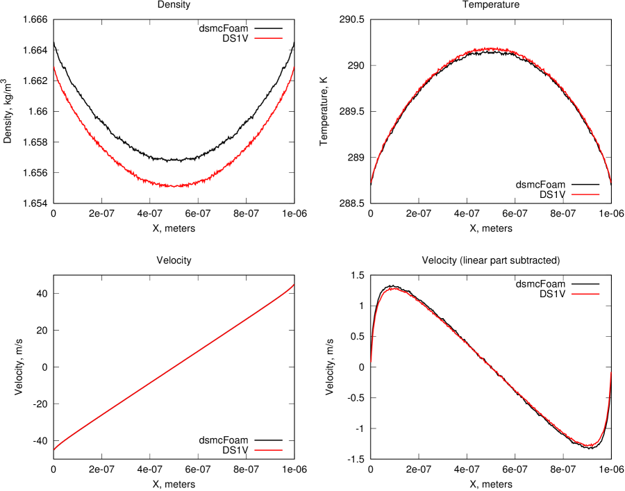
Argon is a monatomic gas, with observed kinetic behavior very close to the ideal gas theory predictions ($\gamma=5/3$, $\mbox{{Pr}}=2/3$). The DSMC computational set-up for the Couette flow for argon was as follows:

• Distance between the walls: $10^{-6}$ meters;

• Difference in wall velocities: 100 meters per second (the coordinate system is chosen so that the left wall moves at $-50$ m/s, while the right wall moves at $50$ m/s);

• Temperature of each wall: 288.15 K (15^∘ Celsius);

• Average number density of argon: $2.5\cdot 10^{25}$ molecules per cubic meter, which corresponds to the argon density $\rho\approx 1.66$ kilogram per cubic meter. This number density is chosen so that the number of molecules is similar to that in the Earth atmosphere at sea level.

Due to slipping, the actual values of the thermodynamic quantities at the boundaries were the following:

• Actual difference in the parallel velocity of the flow at the boundaries: 90.5 meters per second (which set the velocity of the gas flow at the boundaries at $\pm 45.25$ m/s);

• Actual temperature of the flow at each boundary: 288.7 K.

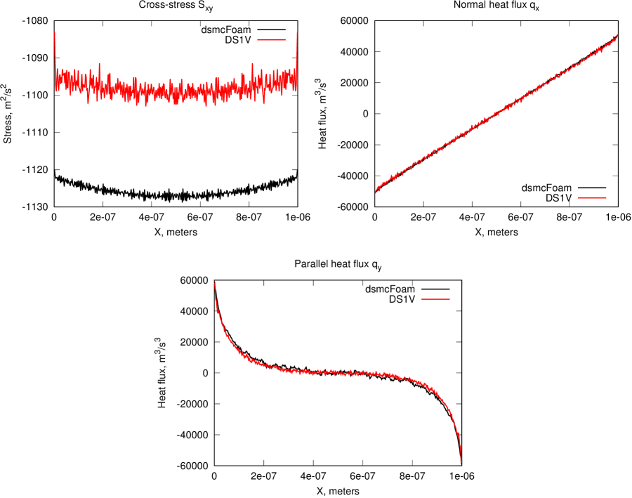
The results of comparison of DS1V and dsmcFoam are shown in Figure 1 for the density, velocity and temperature, and in Figure 2 for the stress and heat flux. Observe that the density, velocity and temperature profiles in Figure 1 are nearly identical (the slight difference in density is likely due to the fact that slightly different numbers of molecules were simulated by DS1V and dsmcFoam). The normal and parallel heat fluxes, shown in Figure 2, are also nearly identical. The discrepancy in the cross-component of the stress in Figure 2 is about 2.5%. Below we use the dsmcFoam as a benchmark for comparison against the fluid dynamics simulations.

For all fluid dynamics equations we used the following parameters for the viscosity and scaled mass diffusivity in (7.1): the molar mass $M$ was set to $3.995\cdot 10^{-2}$ kg/mol for argon, $T^{*}=288.15$ K (that is, 15^∘ C), while the reference constants $\mu^{*}$ and $D_{\alpha}^{*}$ were chosen as follows:

• The reference viscosity $\mu^{*}$ was set to $2.2\cdot 10^{-5}$ kg/(m sec) at 15${}^{\circ}C$ for argon [24, 31].

• The reference mass diffusion coefficient $D_{\alpha}^{*}$ was chosen so that the diffusive Navier-Stokes equations for the Couette flow produced a good correspondence with the DSMC simulation (we found via a few trials that $D_{\alpha}^{*}=4\cdot 10^{-6}$ kg/(m sec) produces a good match).

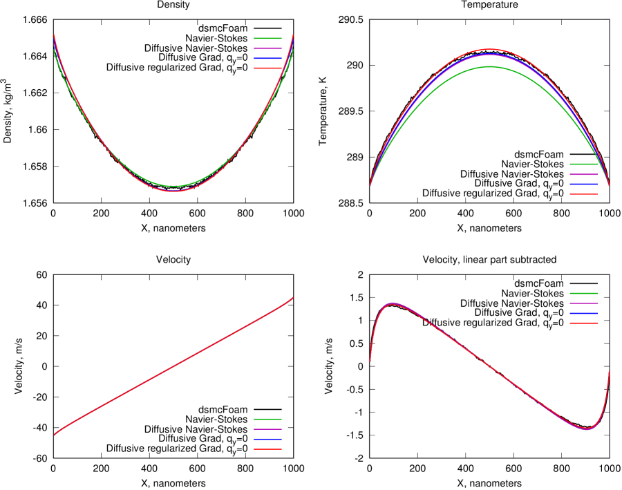
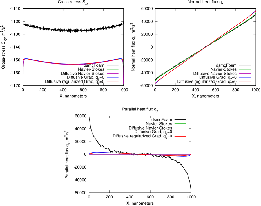
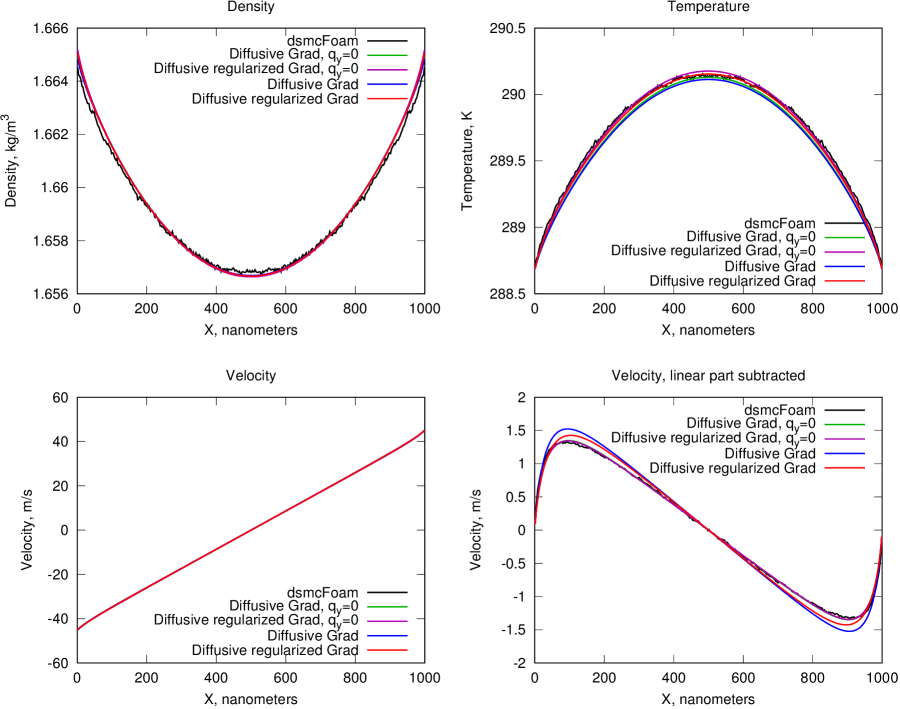
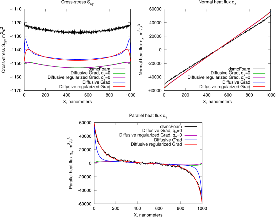
We then carried out the numerical simulations with both the conventional and diffusive Navier-Stokes equations until a steady solution was reached, which we found to occur in about $1.5\cdot 10^{-7}$ seconds. The density, temperature and $y$-velocity profiles, corresponding to both the conventional and diffusive Navier-Stokes equations are compared with the corresponding DSMC profiles in Figure 3. Observe that the density and velocity profiles are captured rather well by both the conventional and diffusive Navier-Stokes equation (note that the velocity exhibits the Knudsen boundary layer thanks to the scaling in (7.2)). However, the temperature is consistently underestimated by the conventional Navier-Stokes equations, while the diffusive Navier-Stokes equations are more accurate in this respect. We can see in Figure 4 that the Newton and Fourier law approximations of the Navier-Stokes equations for the cross-stress and normal heat flux develop irregularities near the walls, which is likely due to the numerical finite difference approximations of the derivatives in the presence of the near-wall mean free path scaling. The parallel heat flux of both the conventional and diffusive Navier-Stokes equations is zero, due to the fact that the problem is translationally invariant along the direction of the flow. Coincidentally, the underestimated temperature of the conventional Navier-Stokes equations produces a better Fourier law approximation to the normal heat flux of the DSMC solution, as also shown in Figure 4. Of course, one has to remember that the DSMC method does not model the exact molecular dynamics in (2.1), and thus the comparisons with an actual measured gas flow need to be done for more definite conclusions.

For the diffusive Grad and regularized diffusive Grad equations, observe that the stress and heat flux boundary conditions need to be provided additionally. We found that setting these additional boundary conditions directly to the values of the corresponding DSMC solution leads to artificial boundary effects, possibly due to the fact that the DSMC computation is not a solution of a partial differential equation, and thus its boundary values are likely inconsistent with the Grad equations. At the same time, the parallel heat flux from the DSMC solution (which is identically zero for the conventional and diffusive Navier-Stokes solutions) cannot simply be ignored.

To investigate this issue, we complete two sets of simulations. First, we compute the solutions of the diffusive Grad and regularized diffusive Grad equations with the boundary conditions for the stress and heat flux chosen so that the corresponding Grad solution matches the one of the diffusive Navier-Stokes equations, to verify that both the diffusive Grad and regularized diffusive Grad equations indeed approximate the diffusive Navier-Stokes equations for this regime. We plot these solutions together with the Navier-Stokes solutions in Figures 3 and 4. Second, we compute the solutions of the diffusive Grad and regularized diffusive Grad equations with the parallel heat flux set to the DSMC value at the boundary, and the rest of the boundary conditions left as described above, to observe the effect of the nonzero parallel heat flux has on the solution. These solutions are plotted in Figures 5 and 6, and compared against the zero parallel heat flux Grad solutions.

Figure 7. The density, velocity and temperature of the Couette flow for nitrogen. The dsmcFoam compared to the DS1V.

Figure 8. The cross-stress, normal heat flux, and parallel heat flux for the Couette flow for argon. The dsmcFoam compared to the DS1V.

Observe that the zero parallel heat flux Grad solutions in Figures 3 and 4 are indeed very good approximations to the diffusive Navier-Stokes equations away from the walls, as all the computed variables are nearly identical. This also suggests that the nonzero parallel heat flux in the DSMC computation is strictly a boundary layer effect (unlike, for example, the normal heat flux or cross-stress), which cannot be reproduced by the Newton and Fourier approximations in (6.14). On the other hand, setting the boundary value of the parallel heat flux to what was computed by the DSMC results in somewhat different behavior between the diffusive Grad and regularized diffusive Grad equations, which we show in Figures 5 and 6. While the diffusive regularized Grad equations approximate the DSMC parallel heat flux rather well, the diffusive Grad equations without the regularization exhibit steeper fall-off of the parallel heat flux (see Figure 6). There is also a very slight “improvement” in the cross-stress component, however, note that it is smaller than the difference between the DS1V and dsmcFoam computations, and thus likely cannot be trusted with certainty. Also, while there is no visibly discernible effect on the temperature or density, the velocity Knudsen boundary layer is slightly “de-tuned”, compared to the DSMC solution, in both the diffusive Grad and regularized diffusive Grad solutions (shown in Figure 5). Given the tiny magnitude of the change, it is, however, unclear whether the Knudsen layer becomes less or more accurate – first, the formula in (7.4) does not necessarily output the exact value of the free mean path, and, second, there is no guarantee that the Knudsen layer of the actual measured gas flow is exactly the same as the one in the DSMC computation.

Figure 9. The density, velocity and temperature of the Couette flow for nitrogen. The boundary parallel heat flux $q_{y}$ for the diffusive Grad and regularized diffusive Grad equations is set to zero.

Figure 10. The cross-stress and heat flux for the Couette flow for nitrogen. The boundary parallel heat flux $q_{y}$ for the diffusive Grad and regularized diffusive Grad equations is set to zero.

Figure 11. The density, velocity and temperature of the Couette flow for nitrogen. Zero vs actual boundary heat flux $q_{y}$ for the diffusive Grad and regularized diffusive Grad equations.

Figure 12. The cross-stress and heat flux for the Couette flow for nitrogen. Zero vs actual boundary heat flux $q_{y}$ for the diffusive Grad and regularized diffusive Grad equations.

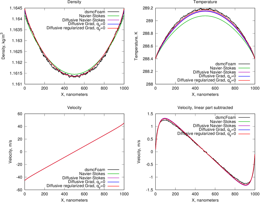
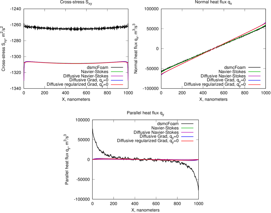
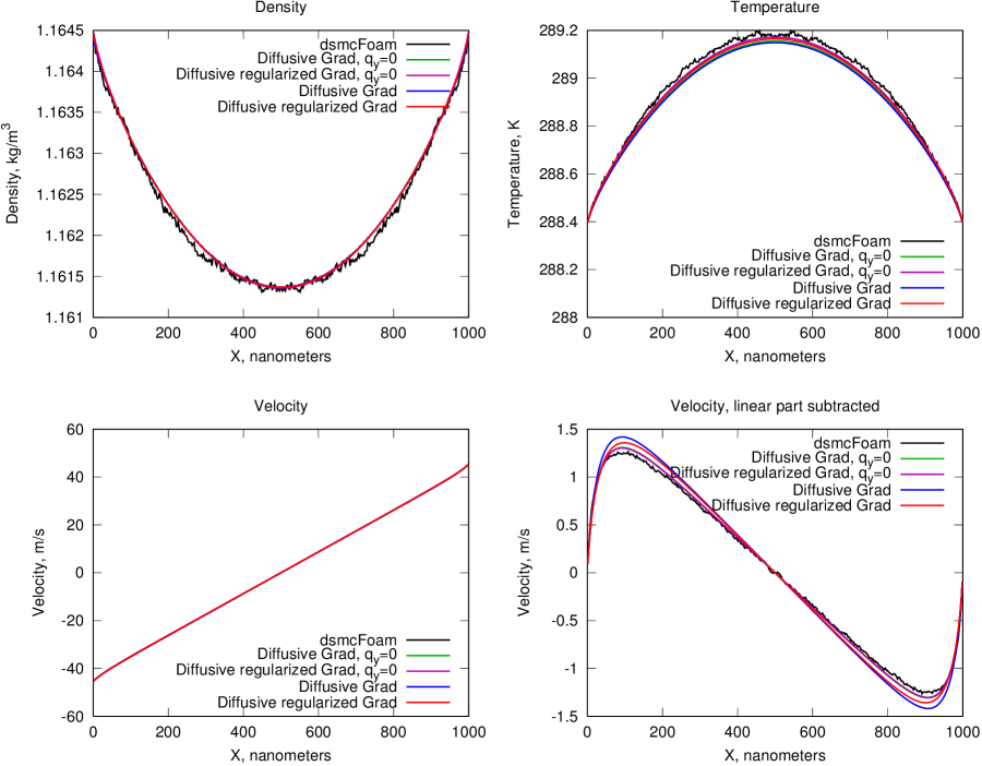
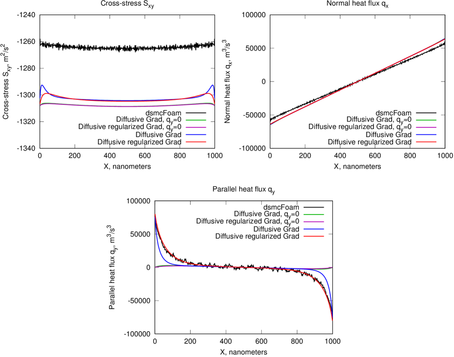
Generally, we conclude from Figures 3–6 that if one does not require the accuracy of the parallel heat flux near the walls, then the diffusive Navier-Stokes equations are already quite accurate for all the other variables, and there is no need to upgrade the model to the nonequilibrium Grad closure. If, however, one requires an accurate approximation for the parallel heat flux, then the regularized diffusive Grad equations should be used, as the diffusive Grad equations without regularization produce the parallel heat flux with a significantly steeper fall-off away from the wall. It appears that the main practical strength of the diffusive and regularized diffusive Grad equations could manifest in situations where significant external heat fluxes are present in the system (for example, modeling the Earth atmosphere with the external surface heat flux appears to be such an application).

7.4. The Couette flow for nitrogen

The DSMC computational set-up for the Couette flow for nitrogen was largely the same as previously for argon:

• Distance between the walls: $10^{-6}$ meters;

• Difference in wall velocities: 100 meters per second;

• Temperature of each wall: 288.15 K (15^∘ Celsius);

• Average number density of nitrogen: $2.5\cdot 10^{25}$ molecules per cubic meter (which corresponds to the nitrogen density $\rho=1.16$ kilogram per cubic meter).

Due to slipping, the actual values of the thermodynamic quantities at the boundaries were the following:

• Actual difference in the parallel velocity of the flow at the boundaries: 90.9 meters per second;

• Actual temperature of the flow at each boundary: 288.4 K.

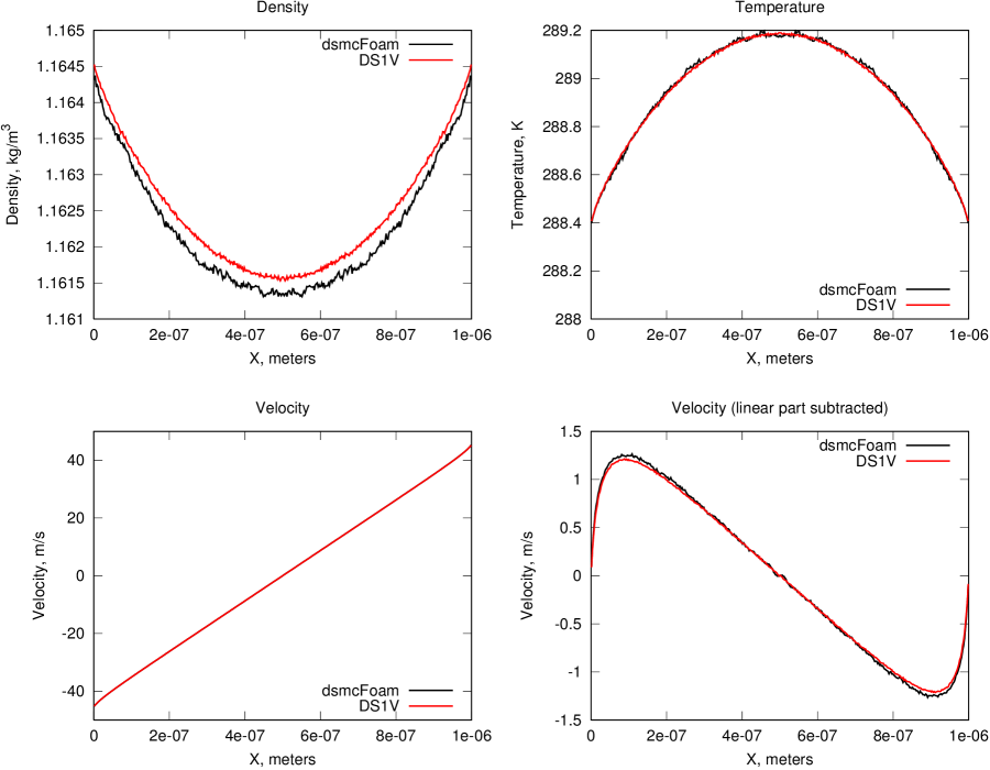
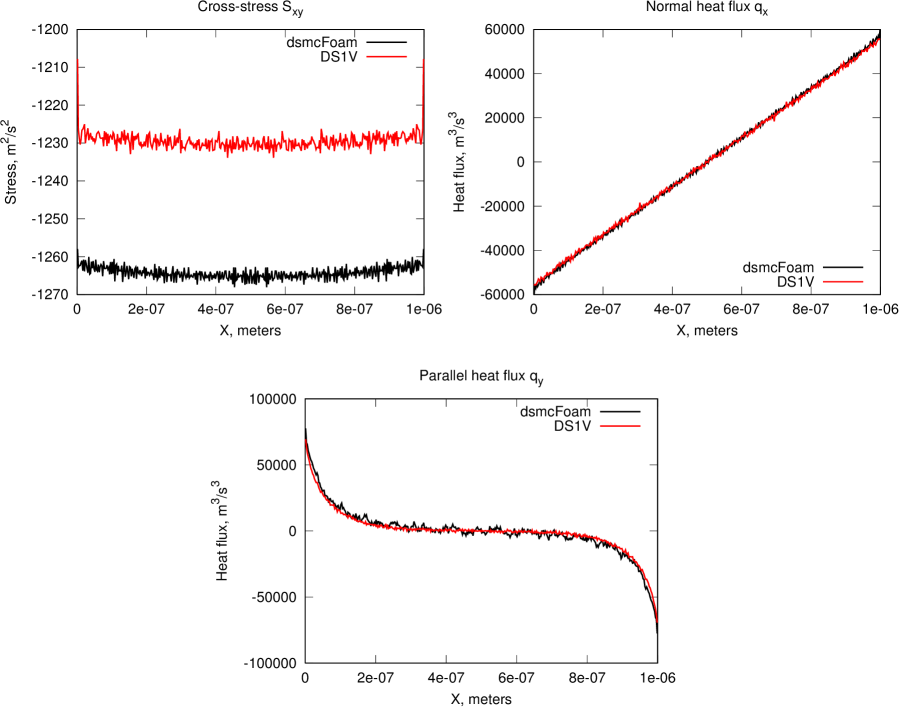
The results of comparison of DS1V and dsmcFoam are shown in Figure 7 for the density, velocity and temperature, and in Figure 8 for the stress and heat flux. Just like previously for argon, here observe that the density, velocity and temperature profiles in Figure 1 are nearly identical (the slight difference in density is likely due to the fact that slightly different numbers of molecules were simulated by DS1V and dsmcFoam). The normal and parallel heat fluxes, shown in Figure 2, are also nearly identical. The discrepancy in the cross-component of the stress in Figure 2 is about 2.5%. As previously for argon, here we use the dsmcFoam as a benchmark for comparison against the fluid dynamics computations.

For both the conventional and diffusive the Navier-Stokes equations we used the same expressions for the viscosity $\mu$ and the scaled mass diffusivity coefficient $D_{\alpha}$ as in (7.1) with the same reference diffusivity constant $D_{\alpha}^{*}=4\cdot 10^{-6}$ kg/(m sec), however, the molar mass $M$ was replaced with that of nitrogen (that is, $2.801\cdot 10^{-2}$ kg/mol) and the reference viscosity constant was set to $1.74\cdot 10^{-5}$ kg/(m sec), which is a standard value for nitrogen at $15^{\circ}$ C [24, 31]. The Prandtl number was set to $\mbox{{Pr}}=0.69$ (also a standard value for nitrogen at 15^∘ C). We then carried out numerical simulations with both the conventional and diffusive Navier-Stokes equations until a steady solution was reached (also about $1.5\cdot 10^{-7}$ seconds). The density, temperature and $y$-velocity profiles, corresponding to both the conventional and diffusive Navier-Stokes equations, are compared with the DSMC profiles on Figure 9. Observe that, just as above for argon, the density and velocity profiles are captured rather well by both the conventional and diffusive Navier-Stokes equations, including the Knudsen boundary layers for the velocity. However, the temperature is consistently underestimated by the conventional Navier-Stokes equations, while the diffusive Navier-Stokes equations are somewhat more accurate. Again, coincidentally, the underestimated temperature of the conventional Navier-Stokes equations produces a better approximation to the normal heat flux of the DSMC solution, as shown in Figure 10. The parallel heat flux of both the conventional and diffusive Navier-Stokes equations is zero, while both the cross-stress and normal heat flux develop irregularities near the walls, likely due to finite difference approximations as above for argon.

For the diffusive Grad and regularized diffusive Grad equations, we complete the two sets of simulations just as above for argon, first one with the boundary values for the stress and heat flux to match the solution of the diffusive Navier-Stokes equations (shown in Figures 9 and 10), and the second one with the parallel heat flux set to the DSMC value at the boundary (shown in Figures 11 and 12). Just as for argon, the zero parallel heat flux Grad solutions shown in Figures 9 and 10 accurately match the solution of the diffusive Navier-Stokes equations away from the walls. However, when the boundary value of the parallel heat flux is set to what was computed by the DSMC, the diffusive regularized Grad equations approximate the DSMC parallel heat flux rather well, while the diffusive Grad equations without the regularization exhibit steeper fall-off of the parallel heat flux (see Figure 12), just as for argon above. The velocity Knudsen boundary layer is again slightly changed, as compared to the DSMC solution, in both the diffusive Grad and regularized diffusive Grad solutions (shown in Figure 11).

Generally, the results in Figures 9–12 match those for argon in Figures 3–6, despite the fact that nitrogen is a gas with a qualitatively different behavior than argon (diatomic, the trace of the stress matrix is nonzero and thus requires a fourteenth equation in the Grad closure). Given the fact that we also re-used the argon values of the higher-order Prandtl numbers for the third and fourth moments in the Grad regularization expressions in (6.23) and (6.24) for nitrogen, the accuracy of the results for nitrogen is quite surprising. It remains to be seen whether the regularized diffusive Grad equations could potentially be used in the modeling of Earth atmosphere in the presence of strong external heat fluxes.

8. Summary

In this work we develop a spatially diffusive analog of the Boltzmann equation, based on the difference between the realistic gas dynamics and the random motion which is modeled by the Boltzmann equation. For that, we first construct a precise multimolecular random process which, in the appropriate limit, leads to the Boltzmann equation. Next, we apply the standard multiscale expansion formalism to the difference dynamics between the realistic gas and the constructed random jump process, and compute the long-term homogenization dynamics for the difference coordinate of a molecule in the form of a diffusion process. We adjust the constructed multimolecular random jump process with this diffusion process, which leads to the Boltzmann equation with an additional spatial diffusion term. We then obtain the hierarchy of the diffusive moment equations from the Boltzmann equation in a standard way, and carry out a computational study of the both the conventional and diffusive Navier-Stokes equations, as well as diffusive and regularized diffusive Grad closures of the moment equations in a simple Couette flow setting with argon and nitrogen. We compare the results with the Direct Simulation Monte Carlo computations. We find that all studied moment closures develop the full-fledged Knudsen velocity boundary layers near the walls, closely matching the results of the DSMC computations. We also note that the conventional Navier-Stokes equations tend to underestimate the temperature away from the walls, while the diffusive Navier-Stokes and Grad closures are more accurate in this respect. Additionally, we find that the component of the heat flux parallel to the flow, produced by the DSMC computations, is captured quite well by the diffusive regularized Grad equations.

For the future study, the natural step forward is to investigate the behavior of the new equations in capillary gas flows under normal conditions, as well as rarefied gas flows, in more advanced spatial configurations. One of the advantages of the new equations is that they combine the ability to model the flows of polyatomic gases (which are ubiquitous in nature) with the higher-order Grad closure, since, to our knowledge, thus far the Grad closure dynamics, where used, were confined to a monatomic set-up. From the kinetic theory perspective, an interesting problem is to estimate the value of the empirical coefficient $\alpha$ in the diffusive scaling (5.6) from the basic principles.

Also, we plan to investigate whether the new equations can be used for modeling turbulent flows in the presence of strong external heat fluxes, such the large scale atmospheric circulation. It is likely that the major benefits of the regularized diffusive Grad approximation should manifest in situations where the heat fluxes are important, since we observed above that the Grad closure demonstrates the ability of capturing both normal and parallel heat fluxes (unlike the Navier-Stokes closures, which can only capture the normal heat flux in the studied set-up). An attractive feature of the diffusive Grad closure is that it allows to prescribe the stress and heat flux at the boundaries explicitly, which could lead to a more detailed model of the energy exchange between the atmosphere and the surface of Earth.

Acknowledgment

The author thanks Ibrahim Fatkullin for interesting discussions, and Jasmine Otto for the help with the OpenFOAM and dsmcFoam software. The work was supported by the Office of Naval Research grant N00014-15-1-2036.

References

- [1] R.V. Abramov. Gas near a wall: a shortened mean free path, reduced viscosity, and the manifestation of a turbulent Knudsen layer in the Navier-Stokes solution of a shear flow. Preprint, 2017, arXiv:1701.02276.
- [2] D. Applebaum. Lévy Processes and Stochastic Calculus. Number 116 in Cambridge Studies in Advanced Mathematics. Cambridge University Press, 2nd edition, 2009.
- [3] G.K. Batchelor. An Introduction to Fluid Dynamics. Cambridge University Press, New York, 2000.
- [4] G.A. Bird. Molecular Gas Dynamics and the Direct Simulation of Gas Flows. Clarendon, Oxford, 1994.
- [5] C. Borgnakke and P.S. Larsen. Statistical collision model for Monte Carlo simulation of polyatomic gas mixture. J. Comput. Phys., 18:405–420, 1975.
- [6] H. Brenner. Kinematics of volume transport. Physica A, 349:11–59, 2005.
- [7] H. Brenner. Navier-Stokes revisited. Physica A, 349:60–132, 2005.
- [8] H. Brenner. Fluid mechanics revisited. Physica A, 370:190–224, 2006.
- [9] C. Cercignani. Theory and Application of the Boltzmann Equation. Elsevier Science, New York, 1975.
- [10] C. Cercignani. The Boltzmann equation and its applications. In Applied Mathematical Sciences, volume 67. Springer, New York, 1988.
- [11] C. Cercignani. Rarefied gas dynamics: From basic concepts to actual calculations. In Cambridge Texts in Applied Mathematics. Cambridge University Press, Cambridge, UK, 2000.
- [12] C. Cercignani, R. Illner, and M. Pulvirenti. The mathematical theory of dilute gases. In Applied Mathematical Sciences, volume 106. Springer-Verlag, 1994.
- [13] S. Chapman and T.G. Cowling. The Mathematical Theory of Non-Uniform Gases. Cambridge Mathematical Library. Cambridge University Press, 3rd edition, 1991.
- [14] P. Courrège. Sur la forme intégro-différentielle des opérateurs de dans satisfaisant au principe du maximum. Séminaire Brelot-Choquet-Deny. Théorie du potentiel, 10(1):1–38, 1965/66.
- [15] S.K. Dadzie and J.M. Reese. Spatial stochasticity and non-continuum effects in gas flows. Phys. Lett. A, 376:967–972, 2012.
- [16] N. Dongari, R. Sambasivam, and F. Durst. Extended Navier-Stokes equations and treatments of micro-channel gas flows. J. Fluid Sci. Tech., 4(2):454–467, 2009.
- [17] S. Duhr and D. Braun. Why molecules move along a temperature gradient. Proc. Natl. Acad. Sci., 103(52):19678–19682, 2006.
- [18] F. Durst, J. Gomes, and R. Sambasivam. Thermofluiddynamics: Do we solve the right kind of equations? In Proceedings of the International Symposium on Turbulence, Heat and Mass Transfer, pages 3–18, Dubrovnik, Croatia, 2006.
- [19] J.W. Gibbs. Elementary Principles in Statistical Mechanics. Charles Scribner’s Sons, New York, 1902.
- [20] I.I. Gikhman and A.V. Skorokhod. Introduction to the Theory of Random Processes. Courier Dover Publications, 1969.
- [21] F. Golse. Evolutionary Equations, volume 2 of Handbook of Differential Equations, chapter The Boltzmann Equation and its Hydrodynamic Limits. Elsevier, 2006.
- [22] H. Grad. On the kinetic theory of rarefied gases. Comm. Pure. Appl. Math., 2(4):331–407, 1949.
- [23] H. Grad. Principles of the kinetic theory of gases. In S. Flügge, editor, Handbuch der Physik, volume 12. Springer, Berlin, 1958.
- [24] J.O. Hirschfelder, C.F. Curtiss, and R.B. Bird. The Molecular Theory of Gases and Liquids. Wiley, 1964.
- [25] K. Itô. Stochastic integral. Proc. Imperial Acad. Tokyo, 20:519–524, 1944.
- [26] K. Itô. On stochastic differential equations. Mem. Amer. Math. Soc., 4:1–51, 1951.
- [27] D. Kelly and I. Melbourne. Deterministic homogenization for fast-slow systems with chaotic noise. Preprint, 2014, arXiv:1409.5748.
- [28] Y. Kifer. L2 diffusion approximation for slow motion in averaging. Stoch. Dyn., 3(2):213–246, 2003.
- [29] Yu.L. Klimontovich. The unified description of kinetic and hydrodynamic processes in gases and plasmas. Phys. Lett. A, 170:434–438, 1992.
- [30] P. Langevin. Sur la théorie du mouvement Brownien. C. R. Acad. Sci. (Paris), 146:530–533, 1908.
- [31] E.W. Lemmon and R.T. Jacobsen. Viscosity and thermal conductivity equations for nitrogen, oxygen, argon, and air. Int. J. Thermophys., 25(1), 2004.
- [32] J.E. Lennard-Jones. On the determination of molecular fields. – II. From the equation of state of a gas. Proc. R. Soc. Lond. A, 106(738):463–477, 1924.
- [33] C.D. Levermore. Moment closure hierarchies for kinetic theories. J. Stat. Phys., 83:1021–1065, 1996.
- [34] F. Mallinger. Generalization of the Grad theory to polyatomic gases. Research Report 3581, Institut National de Recherche en Informatique et en Automatique, 1998. E-print: INRIA-00073100.
- [35] B. Øksendal. Stochastic Differential Equations: An Introduction with Applications. Universitext. Springer, 6th edition, 2010.
- [36] G. Pavliotis and A. Stuart. Multiscale Methods: Averaging and Homogenization. Springer, 2008.
- [37] T.J. Scanlon, E. Roohi, C. White, M. Darbandi, and J.M. Reese. An open source, parallel DSMC code for rarefied gas flows in arbitrary geometries. Comput. Fluids, 39(10):2078–2089, 2010.
- [38] Yu.V. Sheretov. On a regularization of the Boltzmann equation consistent with integral conservation laws. In Application of functional analysis in approximation theory, volume 23, pages 77–92. Tver’ University Press, 2002.
- [39] H. Struchtrup. Grad’s moment equations for microscale flows. AIP Conf. Proc., 663:792–799, 2003.
- [40] H. Struchtrup and M. Torrilhon. Regularization of Grad’s 13-moment equations: Derivation and linear analysis. Phys. Fluids, 15:2668–2680, 2003.
- [41] P.K. Swamee and C.S.P. Ojha. Pump test analysis of confined aquifer. J. Irrig. Drain. Eng., 116(1):99–106, 1990.
- [42] M. Torrilhon and H. Struchtrup. Regularized 13-moment equations: Shock structure calculations and comparison to Burnett models. J. Fluid Mech., 513:171–198, 2004.
- [43] G. Uhlenbeck and L. Ornstein. On the theory of the Brownian motion. Phys. Rev., 36:823–841, 1930.
- [44] E. Vanden-Eijnden. Numerical techniques for multiscale dynamical systems with stochastic effects. Comm. Math. Sci., 1:385–391, 2003.
- [45] V.M. Volosov. Averaging in systems of ordinary differential equations. Russian Math. Surveys, 17:1–126, 1962.