Lattice models for granular-like velocity fields: Hydrodynamic limit

Abstract

A recently introduced model describing -on a 1d lattice- the velocity field of a granular fluid is discussed in detail. The dynamics of the velocity field occurs through next-neighbours inelastic collisions which conserve momentum but dissipate energy. The dynamics can be described by a stochastic equation in full phase space, or through the corresponding Master Equation for the time evolution of the probability distribution. In the hydrodynamic limit, equations for the average velocity and temperature fields with fluctuating currents are derived, which are analogous to those of granular fluids when restricted to the shear modes. Therefore, the homogeneous cooling state, with its linear instability, and other relevant regimes such as the uniform shear flow and the Couette flow states are described. The evolution in time and space of the single particle probability distribution, in all those regimes, is also discussed, showing that the local equilibrium is not valid in general. The noise for the momentum and energy currents, which are correlated, are white and Gaussian. The same is true for the noise of the energy sink, which is usually negligible.

1 Introduction

A fluidised granular material jaeger96 , also referred to as granular fluid, is a substance made of a number of macroscopic particles, or “grains” (e.g. spheres with a diameter of $\sim\!1$mm) which is enclosed in a container and rapidly shaken: the amount of available space and the intensity of the shaking determine the regime of fluidisation puglbook . If the interactions are dominated by two-particles instantaneous (hard-core-like) collisions, one usually speaks of a “granular gas”: in experiments this regime is typically achieved when the peak acceleration is of order of many times the gravity acceleration, and the packing fraction is of order $\sim\!1\%$ or less. The gas regime has played a crucial role in the development of granular kinetic theory: in the dilute limit, one may retrace the classical molecular kinetic theory after having relaxed the constraint of energy conservation BP04 . Granular collisions are, in fact, inelastic: this occurs because each grain is approximated as a rigid body and the collisional internal dynamics is replaced by an effective energy loss (mainly macroscopic kinetic energy cascades into deformations which are finally released as heat).

Granular kinetic theory rests upon many variants of a unique essential model, that of inelastic hard spheres. Important variants include roughness (and rotation), as well velocity-dependent inelastic coefficient, but the smooth-inelastic-hard-sphere model with constant inelasticity is sufficient to explain the basic features of granular gases. The Boltzmann equation for inelastic hard spheres, with numerical solutions and analytical approximations, constitutes the foundation of many investigations in the realm of granular phenomena ne98 . Several procedures have been also proposed to build a granular hydrodynamics, inspired by the idea that a granular fluid can exhibit, in appropriate experimental conditions, a separation between fast microscopic scales and slow macroscopic ones lun84 ; bdks98 . The limits of the granular scale separation hypothesis are more narrow than in the case of molecular gases, for two main reasons: because of the spontaneous tendency of granular gases to develop strong inhomogeneities even at the scale of a few mean free paths and because of the typical small size of a granular system, which is usually constituted by a few thousands of grains goldhirsch ; kadanoff99 . It should be stressed that the latter limitation cannot be easily relaxed even in theoretical studies: stability analysis demonstrated that spatially homogeneous states are unstable for too large sizes ne00 .

The intrinsic size limit of granular gases points out another fundamental requirement for granular kinetic theory: an adequate and consistent description of fluctuations, which are always important in a small system eins ; onsager ; landau . Unfortunately, a general theory for mesoscopic fluctuations in an inherently out-of-equilibrium statistical system does not exist. Important steps in the deduction of a consistent fluctuating hydrodynamics starting from the Boltzmann equation for inelastic hard spheres have been recently taken BMG09 . The framework of Macroscopic Fluctuation Theory Bertini (MFT) is not general enough to address this problem, because it does not include, in its present form, macroscopic equations with advection terms and momentum conservation, such as those in the Navier-Stokes equations that inevitably appear in granular hydrodynamics.

In the last decades, initially outside of the granular realm, lattice models have proved to be a flexible tool to isolate the essential steps in a rigorous approach to the hydrodynamic limit kl ; kmp and its fluctuating version Bertini . Fluctuating hydrodynamics in linear and nonlinear lattice diffusive models have been extensively studied in recent years, both in the conservative Pablo ; Pablo2 ; Pablo3 ; HyK11 and in the dissipative cases for the energy field PLyH12a ; PLyH11a ; PLyH13 . More recently, we have proposed a lattice model for the velocity field of a granular gas, in order to take into account, apart from inelasticity, momentum conservation noi . Momentum conservation appears to be a fundamental ingredient leading to interesting internal structures in the form of long-range correlations grinstein ; correlations . The aim of the present paper is to discuss all the technical details in the derivation of the hydrodynamic equations and the corresponding current fluctuations for that model. Moreover, we report a rich comparison between analytical predictions (from hydrodynamics) and numerical simulations. We also discuss the analogies and the differences between the hydrodynamics of this lattice model and the usual Chapman-Enskog procedure for the Boltzmann equation.

We conclude this introduction by mentioning that the phenomenology of pattern formation in granular gases (such as vortex formation and cluster instability) is reminiscent of swarming and motility induced phase separation in active matter active , which includes complex fluids such as colonies of bacteria or bird flocks. Interestingly, active and granular matter are often associated activegranular ; baskaran . Also in active fluids, the spectacular emergence of spatial patterns, particularly in vectorial fields such as momentum or orientation, is typically understood in terms of hydrodynamic equations active2 . Furthermore, a relevant role is played by fluctuations, as an inevitable consequence of the relative small number of their elementary constituents cgm ; active3 ; rama .

We briefly summarise the organisation of the paper. In the final part of this introduction, section 1.1, we quickly overview some typical regimes observed in the dilute simulations and in the hydrodynamic theory of inelastic hard spheres: such a summary is useful for the uninformed reader, in order to better understand and appreciate the results of our lattice model. In section 2, we introduce the general lattice model, defining it both in terms of stochastic equations and through its Master Equation equivalent description. We also derive a kinetic-like evolution equation for the one-particle distribution function and provide a physical interpretation for the model. In section 3 the balance equations and their hydrodynamic limit are discussed, together with the evolution of the one-particle distribution function in this limit. Section 4 is devoted to the analysis of some relevant physical situations, namely the so-called Homogeneous Cooling, Uniform Shear Flow and Couette flow states. In section 5, we define the current fluctuations and derive the correlations of current noises. The results of numerical simulations of the lattice model are presented and compared with the predictions of our hydrodynamic theory in section 6. Finally, conclusions and perspectives are drawn in section 7. Some technical details, which we omit in the main text, are given in the Appendix.

1.1 Granular hydrodynamics

Full granular hydrodynamics, as derived for instance in bdks98 ; bc01 from the Boltzmann equation for inelastic hard spheres, through a Chapman-Enskog procedure closed at the Navier-Stokes order, consists in the equations for the evolution of three “slow” fields in space coordinates $\vec{r}$ and time $t$: density $n(\vec{r},t)$, velocity $\vec{u}(\vec{r},t)$ and granular temperature $T(\vec{r},t)$. These equations take in generic dimension $d$ the following form

$$\partial_{t}{n}+\nabla\cdot(n\vec{u}) =0,$$ (1a)

$$\partial_{t}{\vec{u}}+\vec{u}\cdot\nabla\vec{u}+(nm)^{-1}\nabla\cdot\mathcal{P} =0,$$ (1b)

$$\partial_{t}{T}+\vec{u}\cdot\nabla T+\frac{2}{dn}\left[\mathcal{P}:(\nabla\vec{u})+\nabla\vec{q}\right]+\zeta T =0,$$ (1c)

with $m$ being the mass of the particles. The “currents” are $\mathcal{P}(\vec{r},t)$ (the pressure tensor) and $\vec{q}(\vec{r},t)$ (the heat flow), reading

$$\mathcal{P}_{ij} =p\delta_{ij}-\eta\left(\nabla_{i}u_{j}+\nabla_{j}u_{i}-\frac{2}{d}\delta_{ij}\nabla\cdot\vec{u}\right),$$ (2a)

$$\vec{q} =-\kappa\nabla T-\mu\nabla n,$$ (2b)

while $\zeta(\vec{r},t)$ (the energy dissipation rate, being $\zeta\to 0$ in the elastic limit), $p$ (the bulk pressure), $\eta$ (the shear viscosity), $\kappa$ (the heat-temperature conductivity) and $\mu$ (the heat-density conductivity) are given by constitutive relations that can be found for instance in bc01 .

We do not intend to describe the many applications of granular hydrodynamics and exhaust the rich catalogue of possible stationary and non-stationary regimes it embraces BP04 ; puglbook . Our aim, here, is just to highlight three essential aspects which constitute the contact points with the model discussed in the rest of the paper: 1) the existence of a spatially homogeneous non-stationary solution, that is, the “Homogeneous Cooling state”, 2) the instability of such a state with respect to shear waves, 3) the existence of the so-called Uniform Shear Flow and Couette flow stationary states. All such aspects descend from a crucial difference with respect to the hydrodynamics of molecular fluids, that is, the presence of the energy sink term $\zeta T$.

When the granular fluid is prepared spatially homogeneous, for instance with periodic boundary conditions, with $n(\vec{r},t)=n$, $u(\vec{r},t)=0$ and $T(\vec{r},t)=T(0)$, (1) are reduced to

$$\dot{T}(t)=-\zeta(t)T(t).$$ (3)

For hard-spheres one has $\zeta(t)\propto T(t)^{1/2}$, which leads to the well known Haff’s law haff

$$T_{\text{\tiny HCS}}(t)=\frac{T(0)}{(1+\frac{\zeta(0)t}{2})^{2}}.$$ (4)

A different collisional model that is often used to simplify the kinetic theory approach is the so-called gas of pseudo-Maxwell molecules ernst81 : its peculiarity is that $\zeta(t)=\zeta(0)$ is constant and therefore the Haff’s law simplifies to an exponential

$$T_{\text{\tiny HCS}}(t)=T(0)\exp[-\zeta(0)t].$$ (5)

The spatially homogeneous solution, with decaying temperature, is generally called “Homogeneous Cooling State” (HCS) and of course can be predicted already from the more fundamental and general level of the Boltzmann breyruiz or even Liouvillebrey_scaling_2007 equation.

The HCS is not stable: when the system is large enough, spatial perturbations of the velocity and density fields can be amplified ne00 . A linear stability analysis shows that the fastest amplification occurs for shear modes, that correspond to a transverse perturbation of the velocity field, for instance a non-zero $y$ component of $\vec{u}$ modulated along the $x$ direction, i.e. $u_{y}(x,t)$. The marginal wave-length $L_{c}$ separating the stable from the unstable regime depends upon the restitution coefficient $\alpha$ as $L_{c}\propto 1/\sqrt{1-\alpha^{2}}$. Notice that the velocity perturbations are not really amplified, because the amplitude of their fluctuations (temperature) always decay: the instability takes place if the rescaled velocity field $u(\vec{r},t)/\sqrt{T_{\text{\tiny HCS}}(t)}$ is considered, i.e. the velocity is divided by the Haff solution. Perturbations in the other fields (density, longitudinal velocity and temperature), which are coupled, are also amplified, but with a slower rate and for larger wavelengths.

There is a range of sizes of the system such as the only linearly unstable mode is the shear mode BP04 : this implies that the velocity field is incompressible and density does not evolve from its initial uniform configuration. Such a regime may be observed for a certain amount of time (longer and longer as the elastic limit is approached). In two dimensions, (1) is obeyed with constant density and, for instance, $u_{x}=0$ whereas the hydrodynamic fields $u_{y}$ and $T$ only depend on $x$, leading to

$$\partial_{t}{u_{y}(x,t)} =(nm)^{-1}\partial_{x}\eta\partial_{x}u_{y}(x,t),$$ (6a)

$$\partial_{t}{T}(x,t) =\frac{1}{n}\eta[\partial_{x}u_{y}(x,t)]^{2}+\frac{1}{n}\partial_{x}\kappa\partial_{x}T(x,t)-\zeta T.$$ (6b)

In section 3 we will see that our lattice model is well described, in the hydrodynamic limit, by the same equations.

It is interesting to put in evidence that (6) sustains also particular stationary solutions. Seeking time-independent solutions thereof, one finds

$$\partial_{x}\eta\partial_{x}u_{y}^{(s)}(x)=0,$$ (7a)

$$\eta[\partial_{x}u_{y}^{(s)}(x)]^{2}=-\partial_{x}\kappa\partial_{x}T^{(s)}(x)+n\zeta T^{(s)}(x).$$ (7b)

The general situation is that both the average velocity and temperature profiles are inhomogeneous: this is the so-called Couette flow state, which also exists in molecular fluids. Yet, in granular fluids, there appears a new steady state in which the temperature is homogeneous throughout the system, $T^{(s)}(x)=T$, and the average velocity has a constant gradient, $\partial_{x}u=a$: this is the Uniform Shear Flow (USF) state, characterised by the equations

$$\partial_{x}^{2}u_{y}^{(s)}(x)=0,$$ (8a)

$$\eta[\partial_{x}u_{y}^{(s)}(x)]^{2}=n\zeta T^{(s)}.$$ (8b)

Such a steady state is peculiar of granular gases where the viscous heating term is locally compensated by the energy sink term. In a molecular fluid, this compensation is lacking and viscous heating must be balanced by a continuous heat flow toward the boundaries, which entails a gradient in the temperature field, typical of the Couette flow.

2 Definition of the model

The model we study here has been introduced in noi and it is inspired by two previous granular models on the lattice, i.e. those in Balbet and PLyH11a . The new model is different from these two previous proposals in a few crucial aspects. In Balbet , the velocity field evolved under the enforcement of the so-called kinematic constraint (see below), which is disregarded here. In PLyH11a , only the energy field was considered, therefore momentum conservation was absent.

2.1 Lattice model in discrete time

The model is, for simplicity, defined on a 1d lattice with $N$ sites, but its generalisation to higher dimension is straightforward. At a given time $p\geq 0$ (time is discrete, i.e. $p\in\mathbb{N}$), each site $l\in[1,N]$ possesses a velocity $v_{l,p}\in$ $\mathbb{R}$.

We start by sketching an informal description of the (Markovian) stochastic dynamics, by introducing how one individual trajectory thereof is built. In each microscopic time step, with a probability discussed below, a pair of nearest neighbours $\left(l,l+1\right)$ collides inelastically and evolves following the rule

$$v_{l,p+1} =v_{l,p}-(1+\alpha)\Delta_{l,p}/2$$ (9a)

$$v_{l+1,p+1} =v_{l+1,p}+(1+\alpha)\Delta_{l,p}/2,$$ (9b)

having defined $\Delta_{l,p}=v_{l,p}-v_{l+1,p}$ and with $0<\alpha\leq 1$. Momentum is always conserved,

$$v_{l,p}+v_{l+1,p}=v_{l,p+1}+v_{l+1,p+1},$$ (10)

while energy, if $\alpha\neq 1$, is not:

$$v^{2}_{l,p+1}+v^{2}_{l+1,p+1}-v^{2}_{l,p}-v^{2}_{l+1,p}=(\alpha^{2}-1)\Delta_{l,p}^{2}/2<0.$$ (11)

The collision rule in (9) is valid for bulk sites, and must be complemented with the suitable boundary conditions for the physical situation of interest. The simplest case is that of periodic boundary conditions, such that if the colliding pair $(N,N+1)$ is chosen, it is equivalent to the pair $(N,1)$. Different boundary conditions, such as thermostats at the boundaries can be easily implemented, of course without any influence for the bulk hydrodynamics. More invasive thermostats can also be conceived, such as the so-called stochastic thermostat that acts on each particle, see puglisi98 ; NETP99 , but we do not consider this possibility here.

Note that (9) is nothing but the particularisation to the one-dimensional case of the simplest collision rule used in granular fluids. More specifically, it corresponds to the model of instantaneous (hard-core) interaction with a constant restitution coefficient, independent of the relative velocity of the particles involved PyL01 .

The evolution equation for the velocities reads

$$v_{l,p+1}-v_{l,p}=-j_{l,p}+j_{l-1,p},$$ (12)

which is a discrete continuity equation for the momentum. The momentum current, that is, the flux of momentum from site $l$ to site $l+1$ at the $p$-th time step reads

$$j_{l,p}=\frac{1+\alpha}{2}\Delta_{l,p}\delta_{y_{p},l}.$$ (13)

Here $\delta_{y_{p},l}$ is Kronecker’s $\delta$ and $y_{p}\in[1,L]$ is a random integer which selects the colliding pair. The number of colliding pairs $L$ is different depending on the choice of boundary conditions. More specifically, for periodic boundary conditions, $L=N$, whereas for thermostatted boundaries $L=N+1$: aside from the $N-1$ “bulk” pairs, end-particles $1$ and $N$ may collide with the boundary particles $0$ and $N+1$, the velocities of which are extracted from a Maxwellian distribution with the corresponding boundary temperature. The variable $y_{p}$ takes the value $l$ with a probability $P_{l,p}$ which basically represents the probability that in the time-step $p$ the nearest-neighbours pair at sites $(l,l+1)$ collides. In our model such a probability is chosen to be of the form

$$P_{l,p}\propto|\Delta_{l,p}|^{\beta},\quad\overline{\delta_{y_{p},l}}=P_{l,p},$$ (14)

with $\beta\geq 0$ a parameter of the model that makes it possible to choose the collision rate. Here, $\overline{\delta_{y_{p},l}}$ denotes an average over all the realisations of the stochastic process compatible with the given values of the velocities. For $\beta=0$, the collision rate is independent of the relative velocity, similarly to the case of pseudo-Maxwell molecules for the inelastic Boltzmann equation Balbet , while $\beta=1$ and $\beta=2$ are analogous to the hard core breyruiz and “very hard-core” ernst81 ; ernst collisions, respectively.

In conclusion, after initial conditions are setup, a given realisation of the random variable $y_{p}$ determines a given realisation of the stochastic process $\vec{v}_{p}\equiv\{v_{1,p},...,v_{N,p}\}$, which is the phase space vector.

For what follows, it is useful to study the corresponding equation for the energy, obtained by squaring (12), with the result

$$v^{2}_{l,p+1}-v^{2}_{l,p}=-J_{l,p}+J_{l-1,p}+d_{l,p}.$$ (15)

Again, we have defined an energy current from site $l$ to site $l+1$ as

$$J_{l,p}=(v_{l,p}+v_{l+1,p})j_{l,p}.$$ (16)

In addition, the energy dissipation at site $l$ is

$$d_{l,p}=(\alpha^{2}-1)[\delta_{y_{p},l}\Delta_{l,p}^{2}+\delta_{y_{p},l-1}\Delta_{l-1,p}^{2}]/4<0.$$ (17)

The total energy of the system at time $p$ is $e_{p}=\sum_{l=1}^{N}v_{l,p}^{2}$.

2.2 Master equation

The stochastic model defined in section 2.1 is a Markov jump process in a continuous phase space $\vec{v}_{p}\in\mathbb{R}^{N}$ with discretised time $p\in\{0,1,2...\}$. A continuous time description may be introduced by assigning a stochastic time increment to the step $p\to p+1$: over each trajectory of the stochastic process, time is increased at the $p$-th step by an amount

$$\delta\tau_{p}=-\frac{\ln\chi}{\Omega_{p}(L)},\quad\Omega_{p}(L)=\omega\sum_{l=1}^{L}|\Delta_{l,p}|^{\beta},$$ (18)

in which $\chi$ is a stochastic variable homogeneously distributed in the interval $(0,1)$ and $\omega$ is a constant frequency that determines the time scale. The physical meaning of the choice (18) is clear: $\Omega_{p}(L)$ is the total exit rate from the state of the system, as given by its velocity configuration $\vec{v}$, at time $p$, and the time increment $\delta\tau$ follows from a Poisson distribution, $P(\delta\tau)=\Omega_{p}(L)\exp[-\Omega_{p}(L)\delta\tau]$.

In order to simplify the writing of the master equation, it is convenient to introduce some definitions. First, analogously to what we did when writing (9), we define $\Delta_{l}$ as

$$\Delta_{l}=v_{l}-v_{l+1},$$ (19)

Second, we introduce the operator $\hat{b}_{l}$, which evolves the vector $\vec{v}$ by colliding the pair $(l,l+1)$, i.e.

$$\hat{b}_{l}(v_{1},...,v_{l},v_{l+1},...,v_{N})=\left(v_{1},...,v_{l}-\frac{1+\alpha}{2}\Delta_{l},v_{l+1}+\frac{1+\alpha}{2}\Delta_{l},...,v_{N}\right).$$ (20)

Also, note of that for a generic function of the velocities $f(\vec{v})$ one has

$$\int d\vec{v}^{\prime}|v^{\prime}_{l}-v^{\prime}_{l+1}|^{\beta}\delta(\vec{v}-\hat{b}_{l}\vec{v}^{\prime})f(\vec{v}^{\prime})=\frac{|\Delta_{l}|^{\beta}}{\alpha^{\beta+1}}f(\hat{b}_{l}^{-1}\vec{v}).$$ (21)

The operator $\hat{b}_{l}^{-1}$ is the inverse of $\hat{b}_{l}$, that is, it changes the post-collisional velocities into the pre-collisional ones when the colliding pair is $(l,l+1)$.

The continuous time Markov process is fully described by the two-time conditional probability $P_{N}(\vec{v},\tau|\vec{v}_{0},\tau_{0})$ with $\tau\geq\tau_{0}$, which evolves according to the following forward Master Equation,

$$\partial_{\tau}P_{N}(\vec{v},\tau|\vec{v}_{0},\tau_{0})=\!\!\int\!d\vec{v}^{\prime}W(\vec{v}|\vec{v}^{\prime})P_{N}(\vec{v}^{\prime},\tau|\vec{v}_{0},\tau_{0})-\Omega(\vec{v})P_{N}(\vec{v},\tau|\vec{v}_{0},\tau_{0}),$$ (22)

in which

$$W(\vec{v}^{\prime}|\vec{v})=\omega\sum_{l=1}^{N}|\Delta_{l}|^{\beta}\delta(\vec{v}^{\prime}-\hat{b}_{l}\vec{v}).$$ (23)

and

$$\Omega(\vec{v})=\int d\vec{v}^{\prime}W(\vec{v}^{\prime}|\vec{v})=\omega\sum_{l=1}^{N}|\Delta_{l}|^{\beta}.$$ (24)

The master equation can be simplified by making use of (21), with the final result

$$\partial_{\tau}P_{N}(\vec{v},\tau|\vec{v}_{0},\tau_{0})=\omega\sum_{l=1}^{L}|\Delta_{l}|^{\beta}\left[\frac{P_{N}(\hat{b}_{l}^{-1}\vec{v},\tau|\vec{v}_{0},\tau_{0})}{\alpha^{\beta+1}}-P_{N}(\vec{v},\tau|\vec{v}_{0},\tau_{0})\right].$$ (25)

The conditional probability distribution $P_{N}(\vec{v},\tau|\vec{v}_{0},\tau_{0})$ is the solution of the above equation with the initial condition $P_{N}(\vec{v},\tau_{0}|\vec{v}_{0},\tau_{0})=\delta(\vec{v}-\vec{v}_{0})$. On the other hand, the one-time probability distribution $P_{N}(\vec{v},\tau)$ verifies the same equation but with an arbitrary (normalised) initial condition $P_{N}(\vec{v},0)$.

Residence time algorithms that give a numerical integration of the master equation in the limit of infinite trajectories bortz_new_1975 ; prados_dynamical_1997 , show that either (22) or (25) is the Master equation for a continuous time jump Markov process consisting in the following chain of events:

1. at time $\tau$, a random “free time” $\tau_{f}\geq 0$ is extracted with a probability density $\Omega(\vec{v}){\exp[-\Omega(\vec{v})\tau_{f}]}$ which depends upon the state of the system $\vec{v}$;

2. time is advanced by such a free time $\tau\to\tau+\tau_{f}$;

3. the pair $(l,l+1)$ is chosen to collide with probability $\omega|\Delta_{l}|^{\beta}/\Omega(\vec{v})$;

4. the process is repeated from step 1.

The connection between the discrete-time stochastic trajectories in  2.1 and the continuous-time master equation here is straightforward, since the former are nothing but the trajectories that integrate the latter in the residence time algorithm.

The Master equation derived above can be considered our “Liouville equation”, that is, it evolves the probability in full phase-space. It is tempting, from such equation, to derive a Lyapunov (or “H”) functional which is minimised by the dynamics, as it is customary for Markov processes vank . However, in the general case our system does not admit an asymptotic steady state, apart from the trivial zero, and therefore the usual H function (which relies upon the existence of the steady state) cannot be built. However, this programme can be carried on in the presence of appropriate boundary conditions, e.g. thermostats, which allow the system to reach a steady state hfun1 ; hfun2 .

2.3 Evolution equation for the one-particle distribution

Here, we apply the usual procedure of kinetic theory and map the Master equation into a BBGKY hierarchy. In particular, we focus on the evolution equation for the one-particle distribution function at site $l$ and at time $\tau$, which we denote by $P_{1}(v;l,\tau)$. By definition,

$$P_{1}(v;l,\tau)=\int d\vec{v}P_{N}(\vec{v},\tau)\delta(v_{l}-v).$$ (26)

It is easy to show that none of the terms in the sum (25) contribute to the time evolution of $P_{1}$ except those corresponding to $l-1$ and $l$, because the collisions involving the pairs $(l-1,l)$ and $(l,l+1)$ are the only ones which change the velocity at site $l$. Therefore,

$$\partial_{\tau}P_{1}(v;l,\tau)=\omega\times$$

$$\left\{\int_{-\infty}^{+\infty}\!\!dv_{l-1}|\Delta_{l-1}|^{\beta}\left[\frac{P_{2}(\hat{b}_{l-1}^{-1}\{v_{l-1},v\};l-1,l,\tau)}{\alpha^{\beta+1}}-P_{2}(v_{l-1},v;l-1,l,\tau)\right]\right.$$

$$\left.\;+\int_{-\infty}^{+\infty}\!\!dv_{l+1}|\Delta_{l}|^{\beta}\left[\frac{P_{2}(\hat{b}_{l}^{-1}\{v,v_{l+1}\};l,l+1,\tau)}{\alpha^{\beta+1}}-P_{2}(v,v_{l+1};l,l+1,\tau)\right]\right\},$$

where, for the sake of simplicity, we also denote by $\hat{b}_{l}^{-1}$ the backward collisional operator which acts on only the velocities of the colliding particles. In the equation above, we have the two-particle probability distribution $P_{2}(v,v^{\prime};l,l+1,\tau)$ for finding the particles at the $l$-th and $(l+1)$-th sites with velocities $v$ and $v^{\prime}$, respectively. For the special case $\beta=0$, the evolution equation for $P_{1}$ can be further simplified, because the terms on the rhs of (2.3) coming from the loss (negative) terms of the master equation can be integrated. We get

$$\partial_{\tau}P_{1}(v;l,\tau)=\omega\left[-2P_{1}(v;l,\tau)+\frac{1}{\alpha}\int_{-\infty}^{+\infty}dv_{l-1}P_{2}(\hat{b}_{l-1}^{-1}\{v_{l-1},v\};l-1,l,\tau)\right.\\ +\left.\frac{1}{\alpha}\int_{-\infty}^{+\infty}dv_{l+1}P_{2}(\hat{b}_{l}^{-1}\{v,v_{l+1}\};l,l+1,\tau)\right].$$ (28)

The equation for $P_{1}$, either (2.3) for a generic $\beta$ or (28) for $\beta=0$, could be converted to a closed equation for $P_{1}$ by introducing the Molecular Chaos assumption, which in our present context means that

$$P_{2}(v,v^{\prime};l,l+1,\tau)=P_{1}(v;l,\tau)P_{1}(v^{\prime};l+1,\tau)+O(L^{-1}).$$ (29)

By neglecting the $O(L^{-1})$ terms in (29), we obtain a pseudo-Boltzmann or kinetic equation for $P_{1}$, which determines the evolution of the one-time and one-particle averages under the assumption of $O(L^{-1})$ correlations. Note that since $L/N\to 1$ for a large system, independently of the boundary conditions, orders of inverse powers of $N$ and $L$ are utterly equivalent.

The structure of the kinetic equation for $P_{1}$ is thus much simpler for the MM case. In particular, we see along the next sections that the evolution equations for the moments are closed under the molecular chaos assumption, without further knowledge of the probability distribution $P_{1}$. This is the reason why, in the remainder of the paper, we restrict ourselves to the MM case $\beta=0$, since the mathematical treatment needed for the $\beta\neq 0$ case is much more complicated and then is deferred to a later paper.

2.4 Physical interpretation

The model, if taken literally, implies that there is no mass transport, particles are at fixed positions and they only exchange momentum and kinetic energy. As discussed in section 1.1, this can be a valid assumption in an incompressible regime which is expected when the velocity field is divergence free, for instance during the first stage of the development of the shear instability, or in the so-called Uniform Shear Flow. We are also disregarding the so-called kinematic constraint, which is fully considered in Balbet : indeed a colliding pair is chosen independently of the sign of its relative velocity, while in a real collision only approaching particles can collide.

Even without the kinematic constraint, our model has a straightforward physical interpretation: the dynamics occurs inside an elongated 2d or 3d channel, the lattice sites represent positions on the long axis, while the transverse (shorter) directions are ignored; the velocity of the particles do not represent their motion along the lattice axis but rather along a perpendicular one. One may easily imagine that the (hidden) component along the lattice axis is of the order of the perpendicular component, but in random direction. On the one hand, this justifies the choice of disregarding the kinematic constraint, while on the other, the collision rate may still be considered proportional to some power $\beta$ of the velocity difference (in absolute value). A fair confirmation of this interpretation comes from the average hydrodynamics equations derived in section 3, which, as anticipated in section 1.1, replicate the transport equations (6) for granular gases in $d>1$ restricted to the shear (transverse) velocity field.

3 Hydrodynamics

In the following section, we derive the hydrodynamic behaviour for $\beta=0$, in which the evolution equations for the averages are closed. Moreover, the MM case makes it possible to grasp the essential points. Nevertheless, in some situations, we also present results for a generic value of $\beta$.

3.1 Microscopic balance equations

We start from the discrete time picture, by considering the stochastic dynamics introduced in section 2.1. Since we are afterwards going to the continuous time limit, one may wonder why not start from the master equation description in section 2.2 or from the kinetic equation for the one-particle distribution in section 2.3. The reason behind this approach is that, apart from being enlightening from a physical point of view, it turns out to be useful for calculating later the properties of the noises appearing in the fluctuating hydrodynamics description, see section 5.

We start by defining, as relevant fields for hydrodynamics, the following local averages over initial conditions and noise realisations:

$$u_{l,p}= \langle v_{l,p}\rangle,$$ (30a)

$$E_{l,p}= \langle v_{l,p}^{2}\rangle,$$ (30b)

$$T_{l,p}= E_{l,p}-u_{l,p}^{2}.$$ (30c)

A few words should be spent for commenting the choice of the relevant fields: in the usual conservative kinetic theory, the velocity and energy fields are naturally “slow” because of their global conservation (recall that there is no density transport in our model, as discussed before in section 2.4). For a granular gas, energy is not necessarily slow: however, when $\alpha$ approaches $1$, as it is in many physical situations, the total energy evolves quite slowly and can be thought of as a quasi-slow variable. In the following, we show that the hydrodynamic limit requires $\alpha\to 1$ if dissipation of energy and diffusion take place over the same time scale. It is important to realise, however, that such an elastic limit is singular here: in $1d$, when $\alpha=1$ the dynamics corresponds to a pure relabelling without mixing or ergodicity.

The microscopic equations for the evolution of averages at time $p$ at site $l$ are obtained by averaging equations (12) and (15):

$$u_{l,p+1}-u_{l,p}=-\langle j_{l,p}\rangle+\langle j_{l-1,p}\rangle,$$ (31)

$$E_{l,p+1}-E_{l,p}=-\langle J_{l,p}\rangle+\langle J_{l-1,p}\rangle+\langle d_{l,p}\rangle.$$ (32)

Introducing the collision probability $P_{l,p}$ defined in (14), for the case of MM we have that $\langle\delta_{y_{p},l}f(\mathbf{v}_{p})\rangle=L^{-1}\langle f(\mathbf{v}_{p})\rangle$ we can write the averages as

$$\langle j_{l,p}\rangle =\frac{1+\alpha}{2L}\langle\Delta_{l,p}\rangle,$$ (33a)

$$\langle J_{l,p}\rangle =\frac{1+\alpha}{2L}\langle\Delta_{l,p}(v_{l,p}+v_{l+1,p})\rangle,$$ (33b)

$$\langle d_{l,p}\rangle =\frac{\alpha^{2}-1}{4L}\langle\Delta_{l,p}^{2}+\Delta_{l-1,p}^{2}\rangle.$$ (33c)

From these equations, it is readily obtained that

$$\langle j_{l,p}\rangle = \frac{1+\alpha}{2L}\left(u_{l,p}-u_{l+1,p}\right)$$ (34a)

$$\langle J_{l,p}\rangle = \frac{1+\alpha}{2L}\left(T_{l,p}-T_{l+1,p}+u_{l,p}^{2}-u_{l+1,p}^{2}\right)$$ (34b)

$$\langle d_{l,p}\rangle = \frac{\alpha^{2}-1}{4L}\Big{[}2T_{l,p}+T_{l+1,p}+T_{l-1,p}$$ (34c)

$$+2\left(u_{l,p}-\frac{u_{l+1,p}+u_{l-1,p}}{2}\right)^{2}+\frac{1}{2}(u_{l+1,p}-u_{l-1,p})^{2}\Big{]}.$$

In order to write the average dissipation, we have neglected $O(L^{-1})$ terms, since we have made use of the molecular chaos approximation, more specifically of the equality $\langle v_{l,p}v_{l\pm 1,p}\rangle=u_{l,p}u_{l\pm 1,p}+O(L^{-1})$.

Had we considered $\beta\neq 0$, we would have had an extra factor $|\Delta_{l,p}|^{\beta}$ in the averages on the rhs of (33). This extra factor would have made it necessary, apart from the “molecular chaos” hypothesis, to use further assumptions about the one-particle distribution function. More specifically, we would have needed to know its shape, at least in some approximation scheme, to calculate the moments in the average currents and dissipation in terms of the hydrodynamic fields $u$ and $T$, that is, the so-called constitutive relations.

3.2 Balance equations in the hydrodynamic limit

Now we assume that $u_{l,p}$ and $E_{l,p}$ are smooth functions of space and time and introduce a continuum, “hydrodynamic”, limit (HL). First, the macroscopic space-time scales $(x,t)$ are defined which are related to the microscopic ones $(l,p)$ through size-dependent factors:

$$x=l/L,\quad t=\omega\tau/L^{2}=p/L^{3}.$$ (35)

Note that both $x$ and $t$ are dimensionless variables. With the identification $f_{l,p}=f(l/L,p/L^{3})$, we say that $f(x,t)$ is a “smooth” function $f(x,t)$ if

$$f_{l\pm 1,p}-f_{l,p}=\pm L^{-1}\partial_{x}f(x,t)+O\left(L^{-2}\right),$$ (36)

$$f_{l,p\pm 1}-f_{l,p}=\pm L^{-3}\partial_{t}f(x,t)+O\left(L^{-6}\right).$$ (37)

It is natural, on the scales defined by the HL, to define the mesoscopic fields $u(x,t)$, $E(x,t)$ and $T(x,t)$ such that

$$u_{l,p} =u(l/L,p/L^{3}),$$ (38a)

$$E_{l,p} =E(l/L,p/L^{3}),$$ (38b)

$$T_{l,p} =T(l/L,p/L^{3}).$$ (38c)

and assume them to be smooth.

Using these definitions and the smoothness assumption, one finds that each discrete spatial derivative in (31) and (32) introduces a $L^{-1}$ leading factor. Then, the difference between the current terms in the balance equations is of the order of $L^{-3}$, because the average currents $\langle j_{l,p}\rangle$ and $\langle J_{l,p}\rangle$ are of the order of $L^{-2}$, as we have discrete derivatives of the currents therein. Those terms, therefore, perfectly balance the $1/L^{3}$ dominant scaling on the left-hand side, i.e. the time-derivative. Since $\langle d_{l,p}\rangle$ is of the order of $(1-\alpha^{2})/L$, to match the scaling $1/L^{3}$ of the other terms, we define the macroscopic inelasticity

$$\nu=(1-\alpha^{2})L^{2},$$ (39)

and assume it to be order $1$ when the limit is taken. This choice automatically implies that when $L\to\infty$ one has $\alpha\to 1$, that is, microscopic collisions are quasi-elastic.

It must be stressed that, from a mathematical point of view, the following results for the average hydrodynamic behaviour become exact in the double limit $\alpha\to 1$, $L\to\infty$ but finite $\nu=(1-\alpha^{2})L^{2}$, provided that the initial conditions are smooth in the sense given by (36). Nonetheless, for a large-size system, the following results will hold over a certain time window, which is expected to increase as its size $L$ increases. A detailed analysis of the conditions for the validity of our hydrodynamic equations is carried out in section 4.4.

By defining the average mesoscopic currents

$$j_{\text{av}}(x,t)=\lim_{L\to\infty}L^{2}\langle j_{l,p}\rangle,\quad J_{\text{av}}(x,t)=\lim_{L\to\infty}L^{2}\langle J_{l,p}\rangle$$ (40)

and the average mesoscopic dissipation of energy

$$d_{\text{av}}(x,t)=\lim_{L\to\infty}L^{3}\langle d_{l,p}\rangle,$$ (41)

one gets the HL of (31) and (32), which are

$$\partial_{t}u(x,t) =-\partial_{x}j_{\text{av}}(x,t),$$ (42a)

$$\partial_{t}E(x,t) =-\partial_{x}J_{\text{av}}(x,t)+d_{\text{av}}(x,t).$$ (42b)

Therein, the average currents and dissipation follow from (40), (41) and (34), with the result

$$j_{\text{av}}(x,t)=-\partial_{x}u(x,t),$$ (43a)

$$J_{\text{av}}(x,t)=-\partial_{x}\left[u^{2}(x,t)+T(x,t)\right],$$ (43b)

$$d_{\text{av}}(x,t)=-\nu T.$$ (43c)

Note that (i) we have replaced $1+\alpha$ by $2$, because $\alpha^{2}=1-\nu L^{-2}$, and we have already neglected $L^{-1}$ terms and (ii) $J_{\text{av}}(x,t)=-\partial_{x}E(x,t)$, with $E(x,t)=u^{2}(x,t)+T(x,t)$, consistently with (30).

Taking into account the above expressions, the following average hydrodynamic equations are obtained,

$$\partial_{t}u(x,t) =\partial_{xx}u(x,t),$$ (44a)

$$\partial_{t}T(x,t) =-\nu T(x,t)+\partial_{xx}T(x,t)+2\left[\partial_{x}u(x,t)\right]^{2}.$$ (44b)

These equations must be supplemented with appropriate boundary conditions for the physical situation of interest. The identification with the granular Navier-Stokes hydrodynamic equations (6) in the shear mode regime is immediate, particularised for the case of constant (time and space-independent) $\kappa$ and $\eta$.

3.3 One-particle distribution in the hydrodynamic limit

In the hydrodynamic limit defined before, the evolution equation for the one-particle distribution function (2.3) can be written in a simpler form. The main idea is the quasi-elasticity of the microscopic dynamics, which stems from (39) or, equivalently, $\alpha=1-L^{-2}\nu/2+O(L^{-4})$ . Then,

$$P_{2}(\hat{b}^{-1}_{l-1}\{v_{l-1},v\};l-1,l,\tau)=P_{2}(v-\frac{\nu}{4L^{2}}\Delta_{l-1},v_{l-1}+\frac{\nu}{4L^{2}}\Delta_{l-1};l-1,l,\tau)$$

$$=\left[1+\frac{\nu}{4L^{2}}\Delta_{l-1}(\partial_{v_{l-1}}-\partial_{v})\right]P_{2}(v,v_{l-1};l-1,l,\tau)+O(L^{-4}).$$ (45)

Moreover, we make use of the molecular chaos assumption (29) and identify

$$P_{1}(v;l,\tau)=P_{1}(v;x=l/L,t=\omega\tau/L^{2}),$$ (46)

that is, we consider $P_{1}$ to be a smooth function of the hydrodynamic space and time variables $x$ and $t$.

Under the hypotheses outlined above, a lengthy but straightforward calculation gives for arbitrary $\beta$ that

$$\partial_{t}P_{1}(v;x,t) = \partial_{x}\int_{-\infty}^{+\infty}dv^{\prime}|v^{\prime}-v|^{\beta}\left[P_{1}(v^{\prime};x,t)\partial_{x}P_{1}(v;x,t)-\right.$$ (47)

$$\qquad\qquad\qquad\qquad\qquad\left.P_{1}(v;x,t)\partial_{x}P_{1}(v^{\prime};x,t)\right]$$

$$-\frac{\nu}{2}\partial_{v}\int_{-\infty}^{+\infty}dv^{\prime}(v^{\prime}-v)|v^{\prime}-v|^{\beta}P_{1}(v^{\prime};x,t)P_{1}(v;x,t).$$

The most important corrections to this equation emanate from finite size effects that give rise to non-zero correlations, i.e. the corrections to the molecular chaos assumption that are expected to be of the order of $L^{-1}$ second . Of course, this equation must be supplemented with suitable boundary conditions depending on the physical state under scrutiny.

If we took moments in (47), we would obtain the hydrodynamic equations for a generic value of $\beta$. It is clear, from the structure of this equation, that these hydrodynamic equations would be not closed and constitutive relations for the momentum and energy currents and the dissipation fields would be needed, as already stated in section 3.1.

Again, for the case $\beta=0$, the equation for $P_{1}$ in the hydrodynamic limit can be simplified,

$$\partial_{t}P_{1}(v;x,t)=\partial_{xx}P_{1}(v;x,t)+\frac{\nu}{2}\partial_{v}\left[(v-u(x,t))P_{1}(v;x,t)\right]$$ (48)

The above equation is not linear for $P_{1}$, since the average momentum is a functional thereof, $u(x,t)=\int_{-\infty}^{+\infty}dv\,vP_{1}(v;x,t)$. Note that, consistently, by taking moments in (48), the average hydrodynamic equations (44) are reobtained. Additionally, the time evolution of higher central moments of the one-particle distribution function, such as

$$\mu_{3}=\langle(v-u)^{3}\rangle,\quad\mu_{4}=\langle(v-u)^{4}\rangle,$$ (49)

can be derived. These moments are particularly relevant to check deviations from the Gaussian behaviour, since for a Gaussian distribution with variance $T$ one has that $\mu_{3}=0$ and $\mu_{4}=3T^{2}$. Their evolution equations are

$$\partial_{t}{\mu}_{3} = -\frac{3}{2}\nu\mu_{3}+\partial_{xx}\mu_{3}+6\,\partial_{x}u\,\partial_{x}T,$$ (50a)

$$\partial_{t}{\mu}_{4} = -2\,\nu\mu_{4}+\partial_{xx}\mu_{4}+8\,\partial_{x}\mu_{3}\,\partial_{x}u+12T(\partial_{x}u)^{2}.$$ (50b)

Again, these evolution equations must be supplemented with appropriate boundary conditions, which depend on the physical situation of interest.

Note that an appealing physical picture for $P_{1}(v;x,t)$ arises in the continuum limit. In fact,

$$P_{1}(v;x,t)\,dv\,dx = \sum_{l=1}^{N}P_{1}(v;l,t)\,dv\,\Delta x\,\Theta(L^{-1}l-x)\Theta(x+dx-L^{-1}l)$$

$$= L^{-1}\sum_{l=1}^{N}P_{1}(v;l,t)\,dv\,\Theta(L^{-1}l-x)\Theta(x+dx-L^{-1}l),$$

in which $\Theta(x)$ is Heaviside step function. The product of Heaviside functions selects the range of $l$’s corresponding to the interval $(x,x+dx)$. Thus, $P_{1}(v;x,t)dv\,dx$ can be interpreted as the fraction of the total number of particles with velocities in the interval $(v,v+dv)$ and positions in the interval $(x,x+dx)$, which makes it neater the connection with the usual kinetic approach. The density of particles may be obtained by integrating $P_{1}(v;x,t)$ with respect to all the velocities, with the result

$$n(x;t)=\int_{-\infty}^{+\infty}dv\,P_{1}(v;x,t)=1,$$ (52)

which reflects nothing but the fact that the particle density in our system is fixed.

4 Physically relevant states

In this section, we analyse some physically relevant states that are typical of dissipative systems such as granular fluids. Specifically, we investigate the Homogeneous Cooling State (HCS), the Uniform Shear Flow (USF) state and the Couette Flow state. The theoretical results obtained throughout are compared to numerical results in section 6.

4.1 The Homogeneous Cooling State

We now focus our attention on the case of spatial periodic boundary conditions, with an initial “thermal condition”: $v_{l,0}$ is a random Gaussian variable with zero average and unit variance, that is, $T_{l,0}\equiv T(x,0)=1$. Starting from this condition, the system typically falls into the so-called Homogeneous Cooling State (HCS), where the total energy decays in time and the velocity and temperature fields remain spatially uniform. In this case, the solution of the average hydrodynamic equations (44) read

$$u(x,t)=0,\qquad T_{\text{\tiny HCS}}(x,t)=T(t=0)e^{-\nu t}.$$ (53)

The exponential decrease of the granular temperature is typical of MM, where the collision frequency is velocity-independent. It replaces the so-called Haff’s law which was originally derived in the HS case, where $T_{\text{\tiny HCS}}\sim t^{-2}$ because $\dot{T}\propto-T^{3/2}$ haff .

The HCS is known to be unstable: it breaks down in too large or too inelastic systems MN93 . In our model and in the hydrodynamic limit, this condition is expected to be replaced by a condition of large $\nu$. The stability is studied by introducing rescaled fields

$$\tilde{u}(x,t)=u(x,t)/v_{\text{th}}(t),\qquad\tilde{T}(x,t)=T(x,t)/T_{\text{\tiny HCS}}(t),$$ (54)

where we have introduced the thermal velocity

$$v_{\text{th}}(t)=\sqrt{T_{\text{\tiny HCS}}(t)},$$ (55)

and linearising them near the HCS, i.e.

$$\tilde{u}(x,t)=\delta\tilde{u}(x,t),\qquad\tilde{T}(x,t)=1+\delta\tilde{T}(x,t).$$ (56)

The analysis of linear equations becomes straightforward by going to Fourier space,

$$\partial_{t}\delta\tilde{u}(k,t)=\frac{\nu-2k^{2}}{2}\delta\tilde{u}(k,t),\qquad\partial_{t}\delta\tilde{T}(k,t)=-k^{2}\delta\tilde{T}(k,t).$$ (57)

Therefore, $\delta\tilde{u}$ is unstable for wave numbers that verify $\nu-2k^{2}>0$. In the continuous variables we are using, the system size is $1$, so that the minimum available wavenumber is $k_{min}=2\pi$. Thus, there is no unstable mode for $\nu$ (lengths) below a certain threshold $\nu_{c}$ ($L_{c}$), with

$$\nu_{c}=8\pi^{2},\quad L_{c}=2\pi\sqrt{2}\left(1-\alpha^{2}\right)^{-1/2}.$$ (58)

On the contrary, for $\nu>\nu_{c}$ ($L>L_{c}$) the HCS is unstable and modes with wave numbers verifying $k<\sqrt{\nu/2}$ increase with time. This instability mechanisms is identical to the one found in granular gases for shear modes Noijeernst . It is important to stress that the amplification appears in the rescaled velocity $\tilde{u}(x,t)$ and not in the velocity $u(x,t)$.

Interestingly, the one-particle distribution function can be exactly calculated in the HCS. Taking into account the homogeneity of the state and the vanishing of the average velocity $u(x,t)$, (48) for $P(v;t)$ simplifies to

$$\partial_{t}P_{1}(v;t)=\frac{\nu}{2}\partial_{v}\left[vP_{1}(v;t)\right].$$ (59)

This equation can be integrated right away to give

$$P_{1}(v;t)=e^{\nu t/2}P_{1}(ve^{\nu t/2};t=0).$$ (60)

Now, we can define

$$\varphi(c;t)=v_{\text{th}}(t)P_{1}(v;t),\quad c=v/v_{\text{th}}(t),$$ (61)

which is the distribution function for the scaled velocity $c$. By combining (60) and (61), we find that this scaled one-particle distribution function does not evolve, i.e.

$$\varphi(c;t)=\sqrt{T(0)}P_{1}(c\sqrt{T(0)};t=0)=\varphi(c;0).$$ (62)

Therefore, the one-particle distribution function would remain Gaussian for all times if it were so initially, as is usually the case. In general, the shape of the initial distribution of velocities is not altered, and it only “shrinks” with the thermal velocity. A similar behaviour was found for elastic Maxwell molecules with annihilation starting from the Boltzmann equation Maynar-annihilation-I .

4.1.1 Perturbation of the HCS: Non-homogeneous cooling

The average hydrodynamic equations (44) are non-linear, but for the MM case we are considering they can be solved for general periodic initial conditions $u(x,0)$ and $T(x,0)$: the evolution of the velocity profile $u(x,t)$ is decoupled from the evolution of the temperature profile $T(x,t)$ and then $u(x,t)$ can be readily obtained. Afterwards, the evolution equation for $T(x,t)$ can be integrated, with the non-linear viscous heating term $(\partial_{x}u)^{2}$ playing the role of a inhomogeneity.

Going to Fourier space, it is easily shown that

$$u(x,t)=\sum_{n=-\infty}^{+\infty}e^{-n^{2}\nu_{c}t/2}e^{ik_{n}x}\hat{u}(k_{n},0),$$ (63)

being $\hat{u}(k,0)$ the Fourier-transform of the velocity at the initial time, and $k_{n}=2\pi n$. This general results shows that the damping coefficient of the $n$-th shear mode is $\nu_{c}n^{2}/2$; therefore, the slowest decaying mode is the first mode $n=1$, which yields the instability of the HCS for $\nu>\nu_{c}$. Note that $\hat{u}(k_{0},0)=0$, since in the center-of-mass frame we have that $\int_{0}^{1}dxu(x,0)=0$ and total momentum is conserved for periodic boundary conditions.

To be concrete, now we consider an initial perturbation that only excites one Fourier mode in the velocity field, whereas the temperature remains homogeneous. We derive the general solution for an arbitrary initial perturbation later in section 4.2. Thus,

$$u(x,0)=u_{0}\sin(2\pi m\,x),\qquad T(x,0)=T_{0}.$$ (64)

being $m$ an integer number. Then, on the one hand the velocity profile can be immediately written by making use of (63) and, on the other, the viscous heating term $(\partial_{x}u)^{2}$ gives rise to two Fourier modes in the evolution of the temperature, corresponding to $n=2m$ and $n=0$. Namely, we have

$$u(x,t) =e^{-m^{2}\nu_{c}t/2}u_{0}\sin(2\pi m\,x),$$ (65a)

$$\begin{split}T(x,t)&=T_{0}e^{-\nu t}+e^{-m^{2}\nu_{c}t}\frac{u_{0}^{2}}{2}m^{2}\nu_{c}\times\\ &\qquad\qquad\qquad\left[\frac{1-e^{-(\nu-m^{2}\nu_{c})t}}{\nu-m^{2}\nu_{c}}+\cos(4\pi m\,x)\frac{1-e^{-(\nu+m^{2}\nu_{c})t}}{\nu+m^{2}\nu_{c}}\right].\end{split}$$ (65b)

It is clearly seen that the presence of a velocity gradient induces the development of a non-homogeneous temperature profile, through the local mechanism of viscous heating.

4.2 The Uniform Shear Flow steady state

Here we consider that our system is sheared at the boundaries: we impose a velocity difference $a$ (shear rate) between the velocities at the left and right ends of the system. This is done by considering the Lees-Edwards boundary conditions Lees-Edwards

$$u(1,t)-u(0,t)=a,\;u^{\prime}(1,t)=u^{\prime}(0,t),\;T(0,t)=T(1,t),\;T^{\prime}(0,t)=T^{\prime}(1,t),$$ (66)

in which the prime stands for the spatial derivative $\partial_{x}$.

With the above conditions, there is a steady solution of the hydrodynamic equations (44) characterised by a linear velocity profile and a homogeneous temperature:

$$u_{s}(x)=a(x-1/2),\quad T_{s}=2a^{2}/\nu.$$ (67)

This steady state is called Uniform Shear Flow and it is peculiar of dissipative systems, in which the continuous energy loss in collisions may compensate the viscous heating. It is interesting to note, on the other hand, that in our system the rheological effects described by Garzó et al. USF-Maxwell ; USF-rheology are not present because the microscopic dynamics is quasi-elastic.

The USF state is expected to be globally stable, in the sense that the system tends to it from any initial condition compatible with the Lees-Edwards boundary conditions. This stems from the energy injection allowing the system to fully explore its phase space, which entails that the H-theorem for the master equation holds hfun1 ; hfun2 . Therefore, the N-particle distribution $P_{N}(\vec{v};x,t)$ approaches the steady solution of the master equation $P_{N}^{(s)}(\vec{v};x)$ corresponding to the USF monotonically as time increases.

For the USF state, the stationary solution of the one-particle distribution function can be solved: we seek a time-independent solution of (48) with the “scaling” form

$$P_{1}^{(s)}(v;x)=T_{s}^{-1/2}\varphi(c),\qquad c=\frac{v-u_{s}(x)}{T_{s}^{1/2}}.$$ (68)

By doing so, we ensure that the probability distribution verifies the appropriate boundary conditions for the USF state,

$$P_{1}(v;x=1,t)=P_{1}(v-a;x=0,t),\quad\partial_{x}P_{1}(v;x=1,t)=\partial_{x}P_{1}(v-a;x=0,t),$$ (69)

from which the Lees-Edwards conditions for the averages directly follow. The resulting equation for $\varphi(c)$ is quite simple, $\varphi^{\prime\prime}(c)+[c\varphi(c)]^{\prime}=0$, in which the prime stands for the derivative with respect to $c$. Thus, $\varphi(c)\propto\exp(-c^{2}/2)$ and the steady one-particle velocity distribution for the USF state reads

$$P_{1}^{(s)}(v;x)=(2\pi T_{s})^{-1/2}\exp\left\{-\frac{[v-u_{s}(x)]^{2}}{2T_{s}}\right\},$$ (70)

i.e. it is a Gaussian with average local velocity $u_{s}(x)$ and temperature $T_{s}$. Of course, the evolution equations for the higher order moments (50) are compatible with Gaussian steady values, $\mu_{3}^{(s)}=0$ and $\mu_{4}^{(s)}=3T_{s}^{2}$.

4.2.1 Transient evolution towards the USF

In this section, we consider the hydrodynamic equations (44) with the Lees-Edwards boundary conditions (66), and look for the general time-dependent solution thereof.

To start with, we consider the deviations of the average velocity and temperature with respect to their USF values, by introducing

$$\delta u(x,t)=u(x,t)-u_{s}(x),\quad\delta T(x,t)=T(x,t)-T_{s}.$$ (71)

The Lees-Edwards boundary conditions for $(u,T)$ are changed into periodic boundary conditions for $(\delta u,\delta T)$. The latter satisfy the equations

$$\partial_{t}{\delta}u=\partial_{xx}\delta u,\quad\partial_{t}{\delta}T=-\nu\delta T+\partial_{xx}\delta T+4a\partial_{x}\delta u+2(\partial_{x}\delta u)^{2}.$$ (72)

Since no linearisation has been done when deriving the above equations from (44), they exactly describe the approach of the system to the USF state. Note that if we set $a=0$ in (72), we reobtain the exact evolution equations for the deviations from the HCS. Therefore, the general solution for the hydrodynamic fields in the HCS correspond to putting $a=0$ in the expressions derived below.

Now, we go to Fourier space by defining

$$\delta u(x,t)=\sum_{n=-\infty}^{+\infty}\hat{u}(k_{n},t)e^{ik_{n}x},\quad\delta T(x,t)=\sum_{n=-\infty}^{+\infty}\hat{T}(k_{n},t)e^{ik_{n}x}.$$ (73)

The initial values for the Fourier components $(\hat{u},\hat{T})$ are given by

$$\hat{u}(k_{n},0)=\int_{0}^{1}dx\,\delta u(x,0)e^{-ik_{n}x},\quad\hat{T}(k_{n},0)=\int_{0}^{1}dx\,\delta T(x,0)e^{-ik_{n}x}.$$ (74)

Recall that (i) $k_{n}=2n\pi$ and (ii) $\hat{u}(k_{0},t)=0$ in the centre of mass frame.

The quadratic term in (72) that stems from viscous heating couples different Fourier modes. More specifically, the evolution equations in Fourier space read

$$\partial_{t}{\hat{u}(k_{n},t)} = -k_{n}^{2}\hat{u}(k_{n},t),$$ (75a)

$$\partial_{t}{\hat{T}(k_{n},t)} = -(\nu+k_{n}^{2})\hat{T}(k_{n},t)+4iak_{n}\hat{u}(k_{n},t)$$ (75b)

$$+\sum_{m=-\infty}^{+\infty}k_{m}(k_{m}-k_{n})\hat{u}(k_{m},t)\hat{u}^{*}(k_{m}-k_{n},t).$$

The solution of the equation for $\hat{u}(k_{n},t)$ can be written straight away; afterwards, this solution is inserted into the equation for $\hat{T}(k_{n},t)$ that is thus transformed into a closed non-homogeneous linear equation. In this way, we obtain that

$$\hat{u}(k_{n},t)=\hat{u}(k_{n},0)e^{-k_{n}^{2}t},$$ (76a)

$$\hat{T}(k_{n},t)=\hat{T}(k_{n},0)e^{-(\nu+k_{n}^{2})t}+4iak_{n}\hat{u}(k_{n},0)e^{-k_{n}^{2}t}\frac{1-e^{-\nu t}}{\nu}$$

$$\;+2e^{-k_{n}^{2}t}\sum_{m=-\infty}^{+\infty}k_{m}(k_{m}-k_{n})\hat{u}(k_{m},0)\hat{u}^{*}(k_{m}-k_{n},0)\frac{e^{-\nu t}-e^{-2k_{m}(k_{m}-k_{n})t}}{2k_{m}(k_{m}-k_{n})-\nu}.$$

Note that there are no unstable modes in the USF of our model: when the denominators in (76) are zero, the numerators also vanish and the corresponding fractions remain finite. This is consistent with the (linear) stability of the USF state of a dilute granular gas of hard spheres described by the Boltzmann equation with respect to perturbations in the velocity gradient (the only possible ones in our model) Garzo-stability-USF . Nevertheless, here the analysis is not restricted to small perturbations, at the level of the hydrodynamic equations the USF is globally stable.

In the transient behaviour described by the hydrodynamic solutions (76), the one-particle distribution is no longer a Gaussian, since a Gaussian with the local, both in space and time, average velocity and temperature does not solve the “kinetic” equation (48). However, on the basis of the $H$-theorem for the $N$-particle distribution $P_{N}(\vec{v};x,t)$, we expect that $P_{1}(v;x,t)$ would approach the Gaussian distribution in (70) as time increases, independently of the initial condition $P_{1}(v;x,0)$. This is consistent with the global stability of the USF state at the level of the hydrodynamic equations discussed above.

4.3 The Couette Flow steady state

As introduced in section 1.1, equation (44) yields a steady state solution when the system is coupled to reservoirs at its boundaries, e.g. when at sites $0$ ($L$) and $N+1$ ($R$) we have two particles with independent normal velocity distributions, with average $u_{L/R}$ and variance $T_{L/R}$. Thus the system is no longer periodic, there are $L=N+1$ colliding pairs and the boundary conditions for the mesoscopic fields read $u(0)=u_{L}$, $u(1)=u_{R}$, $T(0)=T_{L}$ and $T(1)=T_{R}$. It must be stressed that momentum is no longer conserved for this choice of boundary conditions, since in general $u^{\prime}(1,t)\neq u^{\prime}(0,t)$.

The stationary solution for hydrodynamic equations (44), setting symmetric conditions

$$T_{R}=T_{L}=T_{B},\qquad u_{R}=-u_{L}=a/2,$$ (77)

is

$$u(x) =a\left(x-\frac{1}{2}\right),$$ (78a)

$$T(x) =\frac{2a^{2}}{\nu}+\left(T_{B}-\frac{2a^{2}}{\nu}\right)\frac{\cosh\left[\sqrt{\nu}\left(x-1/2\right)\right]}{\cosh\left(\sqrt{\nu}/2\right)}.$$ (78b)

Here, we have put ourselves in the centre of mass frame by considering that $u_{R}=-u_{L}$, and we see that when $T_{B}=2a^{2}/\nu$ the USF state described in section 4.2 is recovered. On the other hand, when $T_{B}\neq 2a^{2}/\nu$, the average velocity profile remains linear but the temperature develops a gradient, because the viscous heating that stems from the velocity gradient is not locally compensated by the energy sink, which is proportional to the temperature. In other words, when $T_{B}=2a^{2}/\nu$, the velocity gradient $a$ is exactly the one needed to satisfy (44) with an homogeneous temperature throughout the system. Otherwise, if the velocity gradient is smaller, the bulk temperature will be lower than that at the boundaries, and vice versa when the velocity gradient is steeper.

These results satisfy the energy balance (42b) required to have a stationary state, namely

$$J_{\text{av}}(x=0)-J_{\text{av}}(x=1)=\nu\int^{1}_{0}dx\,T(x)$$ (79)

where the lhs is the energy flow entering the system at the boundaries and the rhs is the energy loss in collisions.

The one-particle distribution function is not Gaussian in this steady state, except in the case $T_{B}=2a^{2}/\nu$ for which we recover the USF. This can be readily seen by taking into account the time evolution of higher-order-than-two central moments of the velocity, the evolution of which is governed by (50). In the Couette case, we have Gaussian distributions at the boundaries and the appropriate boundary conditions are

$$\mu_{3}(0,t)=\mu_{3}(1,t)=0,\quad\mu_{4}(0,t)=\mu_{4}(1,t)=3T_{B}^{2}.$$ (80)

Equation (50a) shows clearly the point: if the term $\partial_{x}u\,\partial_{x}T\neq 0$, the third central moment $\mu_{3}$ cannot be identically zero in the steady state and the one-particle distribution is non-Gaussian. Therefore, the only steady state with a Gaussian probability distribution in the present model is the USF. We do not write down the theoretical expressions for $\mu_{3}$ and $\mu_{4}$ in Couette’s steady state because they are not particularly illuminating.

4.4 Validity of the hydrodynamic description

There are some analogies between our expansion in terms of $L^{-1}$ and the Chapman-Enskog expansion of the Boltzmann equation. In both cases, terms up to the second order in the gradients (of the order of $k^{2}$, being $k$ the wave vector, in Fourier space) are kept. On the one hand, and from a purely mathematical point of view, in our model (44) becomes exact in the limit $L\to\infty$, but $\nu=(1-\alpha^{2})L^{2}$ of the order of unity, as previously stated. On the other hand, on a physical basis, the hydrodynamic equations are approximately valid whenever the terms omitted upon writing them are negligible against the ones we have kept.

Following the discussion in the preceding paragraph, we must impose that $L\gg 1$. Moreover, we have also to impose that $t\ll L$ in order to have an approximate hydrodynamic description, which stems from the correlations $\langle v_{i}v_{i\pm 1}\rangle$ being of the order of $L^{-1}$ as compared to the granular temperature noi ; second . For example, in the elastic case at equilibrium, the correlations $\langle v_{i}v_{i+k}\rangle$ do not depend on the distance $k$, and therefore $\langle v_{i}v_{i+k}\rangle=-T(L-1)^{-1}$, $\forall k\neq 0$. More specifically, the term proportional to the correlations in the evolution equation for the granular temperature over the microscopic time scale $\tau$ is of the order of $(1-\alpha^{2})L^{-1}$, which must also be negligible against the second spatial derivative terms, of the order of $L^{-2}$. Then, $(1-\alpha^{2})L\ll 1$ must be further imposed when the correlations are neglected in Equations (44). This condition, although less restrictive that $1-\alpha^{2}=O(L^{-2})$, also implies that the microscopic dynamics is quasi-elastic. In a future paper second , we discuss how to relax these conditions and take into account spatial correlations in the system.

5 Fluctuating hydrodynamics

5.1 Definition of fluctuating currents

The size of granular systems is limited both in real experiments and in numerical or theoretical studies, as discussed before, particularly when the instability of the HCS was analysed in section 4.1. Therefore, it is important to investigate finite size effects and the first way to take into account such effects is to develop what is called the fluctuating hydrodynamic description: the microscopic currents are split in two terms, their “main” contribution that depends only on the hydrodynamic variables, and their corresponding “noises”, with zero average.

The main physical idea under the fluctuating hydrodynamics approach is to calculate the averages that lead from the microscopic dynamics to the hydrodynamic equations in two steps. First, the average over the “fast” variables (namely $y_{p}$) is taken, conditioned to given values of the hydrodynamic fields. This defines the “main” contribution to the current, which is still a function of the “slow” hydrodynamic variables. The difference between the microscopic current and its main contribution is the current noise, which by definition has zero average: it is clear that the average value of the microscopic current (both over the “fast” and “slow” variables) coincides with the average of the main contribution (only over the “slow” variables). Specifically, each physical magnitude is written as $x=\overline{x}+\xi^{(x)}$, where $\overline{x}$ is its main contribution and $\xi^{(x)}$ is its noise.

Following the above discussion, we start by splitting the microscopic currents in their main parts and their noises, namely

$$j_{l,p} =\overline{j}_{l,p}+\xi^{(j)}_{l,p},$$ (81a)

$$J_{l,p} =\overline{J}_{l,p}+\xi^{(J)}_{l,p},$$ (81b)

$$d_{l,p} =\overline{d}_{l,p}+\xi^{(d)}_{l,p}.$$ (81c)

As stated above, overlined variables correspond to partial averages over the fast variables $y_{l,p}$ conditioned to given values of the slow ones $v_{l,p}$. Consequently,

$$\overline{j}_{l,p} =\frac{1+\alpha}{2L}\Delta_{l,p},$$ (82a)

$$\overline{J}_{l,p} =\frac{1+\alpha}{2L}\Delta_{l,p}(v_{l,p}+v_{l+1,p})$$ (82b)

$$\overline{d}_{l,p} =\frac{\alpha^{2}-1}{4L}(\Delta_{l,p}^{2}+\Delta_{l-1,p}^{2}).$$ (82c)

It is clear that such choices guarantee that all noises $\xi^{(j)}$, $\xi^{(J)}$ and $\xi^{(d)}$ have zero average.

5.2 Noise correlations

5.2.1 Noise correlations: momentum current

We start by studying the properties of the current noise correlation function $\xi^{(j)}_{l,p}=j_{l,p}-\overline{j}_{l,p}$, namely the moment $\langle\xi^{(j)}_{l,p}\xi^{(j)}_{l^{\prime},p^{\prime}}\rangle$, which reads

$$\langle\xi_{l,p}^{(j)}\xi_{l^{\prime},p^{\prime}}^{(j)}\rangle=\langle j_{l,p}j_{l^{\prime},p^{\prime}}\rangle-\langle\overline{j}_{l,p}\overline{j}_{l^{\prime},p^{\prime}}\rangle.$$ (83)

In order to obtain the noise correlations, we exploit a series of conditions. First, it is straightforward that $\langle\xi^{(j)}_{l,p}\xi^{(j)}_{l^{\prime},p^{\prime}}\rangle=0$ for $p\neq p^{\prime}$, because $y_{p}$ and $y_{p^{\prime}}$ are independent random numbers. For equal times, $p=p^{\prime}$, the second term on the right hand of (83) is negligible because it is $O(L^{-2})$, while the leading behaviour of the first term will be shown to be $O(L^{-1})$. Using now the definition (13) of the microscopic momentum current, we get

$$j_{l,p}j_{l^{\prime},p^{\prime}}=\frac{(1+\alpha)^{2}}{4}\Delta_{l,p}\delta_{y_{p},l}\Delta_{l^{\prime},p^{\prime}}\delta_{y_{p}^{\prime},l^{\prime}}.$$ (84)

Second, we take into account that

$$\langle\delta_{y_{p},l}\delta_{y_{p},l^{\prime}}\rangle=\delta_{l,l^{\prime}}\langle\delta_{y_{p},l}\rangle=\frac{\delta_{l,l^{\prime}}}{L}.$$ (85)

Thus, for $p=p^{\prime}$, we have

$$\langle\xi_{l,p}^{(j)}\xi_{l^{\prime},p}^{(j)}\rangle=\frac{\left(1+\alpha\right)^{2}}{4L}\left\langle\Delta_{l,p}^{2}\right\rangle\delta_{l,l^{\prime}}+O(L^{-2}).$$ (86)

At this point, we can make use of (i) the quasi-elasticity of the microscopic dynamics to substitute $(1+\alpha)/2$ by $1$ (neglecting terms of order $L^{-2}$) and (ii) the molecular chaos assumption to obtain $\langle\Delta_{l,p}^{2}\rangle$, with the result

$$\langle\Delta_{l,p}^{2}\rangle=T_{l,p}+T_{l+1,p}+(u_{l,p}-u_{l+1,p})^{2}+O(L^{-1})\sim 2T_{l,p},$$ (87)

because both $u_{l+1,p}-u_{l,p}$ and $T_{l+1,p}-T_{l,p}$ are of the order of $L^{-1}$. Therefore,

$$\langle\xi_{l,p}^{(j)}\xi_{l^{\prime},p^{\prime}}^{(j)}\rangle\sim\frac{2}{L}T_{l,p}\,\delta_{l,l^{\prime}}\,\delta_{p,p^{\prime}}.$$ (88)

In the large size system, $j_{l,p}$ scales as $L^{-2}$, as given by (40) (an analogous scaling has been found in other simple dissipative models, see  PLyH12a ). Therefore, the mesoscopic noise of the momentum current is defined as

$$\xi^{(j)}(x,t)=\lim_{L\to\infty}L^{2}\xi_{l,p},\quad j(x,t)=\overline{j}(x,t)+\xi^{(j)}(x,t)$$ (89)

in which, again, $\overline{j}(x,t)=\lim_{L\to\infty}L^{2}\overline{j}_{l,p}$. Going to the continuous limit and remembering (35), which implies that

$$\delta_{l,l^{\prime}}/\Delta x\sim\delta(x-x^{\prime}),\quad\delta_{p,p^{\prime}}/\Delta t\sim\delta(t-t^{\prime}),$$ (90)

we derive the noise amplitude of the momentum current as

$$\langle\xi^{(j)}(x,t)\xi^{(j)}(x^{\prime},t^{\prime})\rangle\sim 2L^{-1}\,T(x,t)\,\delta(x-x^{\prime})\delta(t-t^{\prime}).$$ (91)

5.2.2 Noise correlations: energy current

As in the previous subsection, we start with (81b). Again in this case we are interested in the correlation properties of the noise $\xi^{(J)}_{l,p}=J_{l,p}-\overline{J}_{l,p}$

$$\langle\xi^{(J)}_{l,p}\xi^{(J)}_{l^{\prime},p^{\prime}}\rangle=\langle J_{l,p}J_{l^{\prime},p^{\prime}}\rangle-\langle\overline{J}_{l,p}\overline{J}_{l^{\prime},p^{\prime}}\rangle.$$ (92)

Similarly to the case of the current noise, we have that (i) $\langle\xi^{(J)}_{l,p}\xi^{(J)}_{l^{\prime},p^{\prime}}\rangle=0$ for $p\neq p^{\prime}$, (ii) the second term on the right-hand side is $O(L^{-2})$ and thus subdominant in the limit $L\rightarrow\infty$ and (iii) the noise correlation is dominated by the contribution that stems from the first term on the rhs. Therefore, making use of (16), one gets

$$\langle\xi^{(J)}_{l,p}\xi^{(J)}_{l^{\prime},p}\rangle\sim\langle\delta_{y_{p},l}\delta_{y_{p},l^{\prime}}(v_{l,p}^{2}-v_{l+1,p}^{2})(v_{l^{\prime},p}^{2}-v_{l^{\prime}+1,p}^{2})\rangle,$$ (93)

which will be shown to be of the order of $L^{-1}$. Using once more (85), we obtain

$$\langle\xi_{l,p}^{(J)}\xi_{l^{\prime},p^{\prime}}^{(J)}\rangle\sim\frac{1}{L}\left\langle\left(v_{l,p}^{2}-v_{l+1,p}^{2}\right)^{2}\right\rangle\delta_{l,l^{\prime}}\delta_{p,p^{\prime}}.$$ (94)

In general, the moment $\left\langle\left(v_{l,p}^{2}-v_{l+1,p}^{2}\right)^{2}\right\rangle$ is not a function of the hydrodynamic variables $u$ and $T$, unless the one-particle distribution is Gaussian.

In order to obtain a closed fluctuating hydrodynamic description, we need to write $\langle(v_{l,p}^{2}-v_{l+1,p}^{2})^{2}\rangle$ in terms of the hydrodynamic variables. In order to do so, on top of the molecular chaos assumption (factorisation of the moments involving several sites), we introduce the so-called local equilibrium approximation (LEA): the one-particle distribution function $P_{1}$ is assumed to be the equilibrium distribution corresponding to the local values of the hydrodynamic variables, which in our case corresponds to a Gaussian distribution of the velocities. In some dissipative models without momentum conservation PLyH11a ; PLyH12a ; PLyH13 , there is strong numerical evidence that the LEA gives a good quantitative description of the noise amplitudes, as a consequence of the quasi-elasticity of the underlying microscopic dynamics. In our model, we know that the LEA is not an approximation but an exact result for some physical states, such as the HCS Gaussian_HCS or the USF, but still remains an approximation for other states like the Couette flow.

In the large system size limit, $J_{l,p}$ scales as $L^{-2}$ and it is expected that the noise does too. Along the same lines as in the preceding section, after using the LEA and neglecting terms of the order of $L^{-2}$, we obtain the autocorrelation of the energy current noise,

$$\langle\xi^{(J)}(x,t)\xi^{(J)}(x^{\prime},t^{\prime})\rangle\sim 4L^{-1}T(x,t)[T(x,t)+2u^{2}(x,t)]\delta(x-x^{\prime})\delta(t-t^{\prime}).$$ (95)

Thus, the energy current noise is also white and its amplitude scales as $L^{-1}$ with the system size $L$, accordingly with the physical intuition.

5.2.3 Noise correlations: dissipation field

Now we deal with the third “current” in the system, the dissipation field $d_{l,p}$ by repeating the same procedure as before. We are interested in the correlation properties of the noise $\xi^{(d)}_{l,p}=d_{l,p}-\overline{d}_{l,p}$.

Once more, $\langle\xi^{(d)}_{l,p}\xi^{(d)}_{l^{\prime},p^{\prime}}\rangle=0$ for $p\neq p^{\prime}$ and the dominant contribution for $p=p^{\prime}$ comes from the dissipation correlation $\langle d_{l,p}d_{l^{\prime},p}\rangle$. Making use of the definition of (17),

$$\langle d_{l,p}d_{l^{\prime},p}\rangle = \frac{(\alpha^{2}-1)^{2}}{16L}\left[\delta_{l,l^{\prime}}\langle(v_{l,p}-v_{l+1,p})^{4}+(v_{l-1,p}-v_{l,p})^{4}\rangle+\right.$$ (96)

$$\qquad\left.\delta_{l,l^{\prime}-1}\langle(v_{l,p}-v_{l+1,p})^{4}\rangle+\delta_{l,l^{\prime}+1}\langle(v_{l-1,p}-v_{l,p})^{4}\rangle\right].$$

Therefore, by taking into account the LEA and neglecting $O(L^{-2})$ terms,

$$\langle\xi^{(d)}_{l,p}\xi^{(d)}_{l^{\prime},p^{\prime}}\rangle\sim\frac{3(\alpha^{2}-1)^{2}}{4L}T_{l,p}^{2}[2\delta_{l,l^{\prime}}+\delta_{l,l^{\prime}-1}+\delta_{l,l^{\prime}+1}]\delta_{p,p^{\prime}}.$$ (97)

In the large size system $d_{l,p}$ scales as $L^{-3}$ and we expect the same scaling for the noise. Going to the continuous limit, using again (90), we get

$$\langle\xi^{(d)}_{l,p}\xi^{(d)}_{l^{\prime},p^{\prime}}\rangle\sim L^{-3}\,3\nu^{2}T(x,t)^{2}\delta(x-x^{\prime})\delta(t-t^{\prime}).$$ (98)

In summary, the noise of the dissipation is subdominant with respect to the moment and energy currents, its amplitude being proportional to $L^{-3}$, and therefore it is usually negligible.

5.2.4 Cross-correlations of the noises and Gaussianity

Interestingly, being in the presence of two fluctuating fields, correlations between different noises appear. The cross correlations between different noises are straightforwardly obtained, along similar lines:

$$\langle\xi^{(j)}(x,t)\xi^{(J)}(x^{\prime},t^{\prime})\rangle = \frac{4T(x,t)u(x,t)}{L}\delta(x-x^{\prime})\delta(t-t^{\prime}),$$ (99a)

$$\langle\xi^{(j)}(x,t)\xi^{(d)}(x^{\prime},t^{\prime})\rangle = 0,$$ (99b)

$$\langle\xi^{(J)}(x,t)\xi^{(d)}(x^{\prime},t^{\prime})\rangle = 0,$$ (99c)

up to and including $O(L^{-1})$. Theoretical predictions for noise correlations, amplitudes and Gaussianity have been successfully tested in simulations, see section 6.

Gaussianity of these noises is demonstrated in the Appendix. The proof is similar to that presented in Ref. PLyH12a for a dissipative model with only one field and thus without moment conservation. Interestingly, this proof shows that the Gaussian character of the noises remains valid even if the “local equilibrium approximation” cannot be used to calculate the averages appearing in their amplitudes. Should it be the case, a more sophisticated theoretical approach will be needed to give these amplitudes in terms of the hydrodynamic fields but the noises will still be Gaussian.

6 Numerical results

6.1 General simulation strategy

Simulations have been made reproducing $M$ times the phase-space trajectory of a system of $N$ particles, each one carrying a velocity $v_{l}$ and being at a definite position $l=1,\ldots,L$, with $L=N$ for periodic or Lees-Edwards boundaries and $L=N+1$ for a thermostatted system. For each trajectory, the system starts with a random extraction of velocities $v_{l}$ normally distributed with $\left\langle v_{l}\right\rangle=0$ and $\left\langle v^{2}_{l}\right\rangle=T_{0}$, unless otherwise specified. Afterwards, we move to the centre of mass frame making the transformation $v_{l}\Rightarrow v^{\prime}_{l}=v_{l}-\frac{1}{L}\sum^{L}_{l=1}v_{l}$, so that the total momentum of the system is zero.

We carry out Monte Carlo simulation of the system time-evolution through the residence time algorithm described in section 2.2 bortz_new_1975 ; prados_dynamical_1997 . This procedure allows us to compute the time-evolution of our model for every collision rate $\beta$, although we focus here mainly on the case $\beta=0$ (MM).

Throughout this numerical section, we always plot the scaled one-particle distribution defined as

$$\varphi(c;x,t)=\sqrt{T(x,t)}P_{1}(v;x,t),\quad c=\frac{v-u(x,t)}{\sqrt{T(x,t)}},$$ (100)

in order to avoid visualising the much sharper distributions that arise in some situations as a consequence of the cooling. Note that this definition includes as particular cases (61) for the HCS, in which $u=0$, and (68) for the USF steady state.

6.2 Homogeneous cooling state

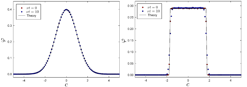
Figure 1: (Colour online) Time evolution of the scaled one-particle distribution function $\varphi(c)$, defined in (100), in the HCS. The shape of the distribution does not evolve with time, remaining unaltered as a function of the scaled velocity $c=v/v_{\text{th}}(t)$ defined in (61). The two panels correspond to two different initial shapes for $P_{1}(v;0)$: the left (right) panel shows the time evolution of a Gaussian (square) distribution. We have averaged over $10^{4}$ realisations, in a system with $N=500$ and $\nu=20$. Small finite-size deviations from the initial shape are observed, mainly for the square distribution.

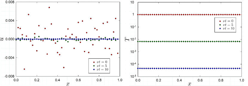
Figure 2: Left: (Colour online) Numerical results (points) and theoretical predictions (lines) for the average velocity profile $u(x,t)$ in the HCS, with $\nu=20<\nu_{c}$, $N=500$, $T_{0}=1$ for different times $\nu t=0$, $5$, $10$. The cooling of the system is clearly shown by the decreasing fluctuations. Right: Same plot for the temperature profile $T(x,t)$ of the system. Averages have been taken over $M=10^{5}$ trajectories.

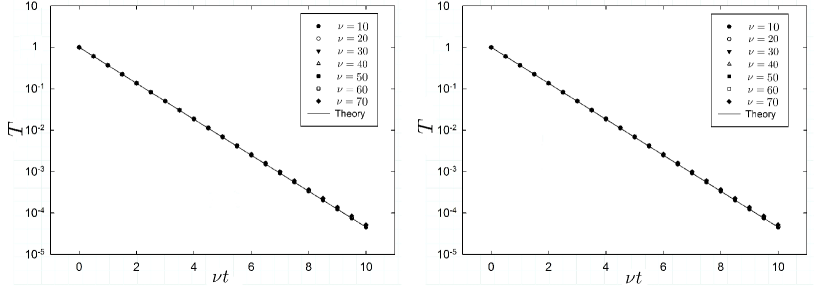
Figure 3: Average temperature versus time in the HCS for several $\nu$ with $N=500$ sites: comparison between numerical values (single points) and the theoretical prediction (53), $T(t)=T_{0}e^{-\nu t}$ (black line). The left panel corresponds to an initial “standard” state with a Gaussian distribution, whereas the right panel shows the plot for an initial square distribution. Averages in both panels correspond to $M=10^{4}$ trajectories.

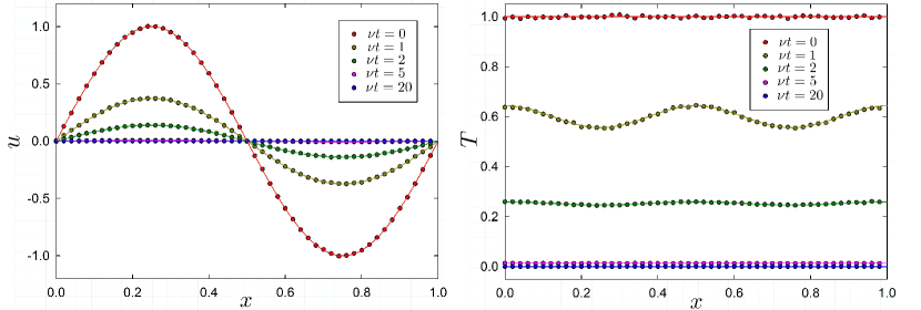
Figure 4: Left: (Colour online) Numerical results (points) and theoretical values (solid lines) for the average sinusoidal velocity profile $u(x,t)$, with $u_{0}=1$, $\nu=40$, $N=500$, $T_{0}=1$ and $m=1$ for $\nu t=0,1,2,5,20$. Right: Same plot for the temperature profile $T(x,t)$ of the system. Here, the averages have been taken over $M=10^{5}$ trajectories.

Following the above-mentioned procedure, we have simulated the homogeneous cooling state described in section 4.1 with periodic boundaries and starting from a flat velocity profile $u(x,0)\equiv 0$ with unit variance $T(x,0)\equiv T_{0}=1$. The comparison between numerical values and analytical expectation is excellent, especially for $\nu\approx 2\pi^{2}$. For this value ($\simeq 20$), it can be shown noi ; second that finite-size corrections stemming from correlations, as discussed in section 4.4, are almost negligible. We mainly consider the initial distribution function to be Gaussian, except for some clearly stated cases, in which the analysis starts from an initial square distribution

$$P_{1}(v;t=0)=\frac{1}{2v_{0}}\Theta(v_{0}-|v|),$$ (101)

being $\Theta(v)$ the Heaviside step function. The parameter $v_{0}$ is adjusted in order to have unit variance ($v_{0}=\sqrt{3}$).

For the HCS, we have shown that the one-particle distribution function $P_{1}(v;t)$ conserves its initial shape, as given by (62). We check numerically here this result, by considering two initial velocity distributions, Gaussian and square, for $\nu=20$. In figure 1, we compare this theoretical prediction with numerical results, finding excellent agreement except for very small finite-size corrections.

Figures 2 and 3 show the time evolution of the hydrodynamic variables $u$ and $T$. In figure 2, the profiles $u(x,t)$ and $T(x,t)$ are displayed for different times, as a function of the spatial coordinate $x$, again for $\nu=20$. It is clearly observed that the system remains spatially homogeneous while it cools. On the other hand, the Haff law is checked in figure 3 for different values of $\nu$ below the critical threshold $\nu_{c}=8\pi^{2}$: the agreement is excellent, whether the initial one-particle velocity distribution is Gaussian (left) or square (right).

Also, we have performed simulations of non-homogeneous cooling, starting as in section 4.1.1 from a sinusoidal periodic average velocity profile $u(x,0)=u_{0}\sin(2\pi mx)$, with $m$ integer, and a homogeneous temperature $T(x,0)=T_{0}=1$ as before. The simulations show the cooling of the system, as expected from (65), with the development of a temperature profile given by viscous heating. Comparisons between numerical results and theoretical predictions for the non-homogeneous case are displayed in figure 4.

6.2.1 Instability of the HCS

It is possible to observe numerically the instability of the HCS predicted in section 4.1 by simulating a weakly perturbed system and looking at the time behaviour of the rescaled average velocity $\tilde{u}(x,t)=u(x,t)/\sqrt{T_{\text{\tiny HCS}}(t)}$. We have obtained the trajectories of a system starting with the same sinusoidal profile as in (64) and observing the time-evolution of the maximum $u_{M}(t)=u(x_{M},t)$. From (65a), we have that $u_{M}\sim e^{-\nu_{c}t/2}$, yielding $\tilde{u}_{M}(t)=u_{0}e^{(\nu-\nu_{c})t/2}$. Hence, we should recover the instability of the homogeneous cooling state for $\nu>\nu_{c}=8\pi^{2}$. In this range of values of $\nu$, shear modes of the rescaled velocity begin to be amplified and thus the system develops inhomogeneities. In figure 5, we show numerical results for this rescaled average velocity, which confirm the existence of the threshold $\nu_{c}$.

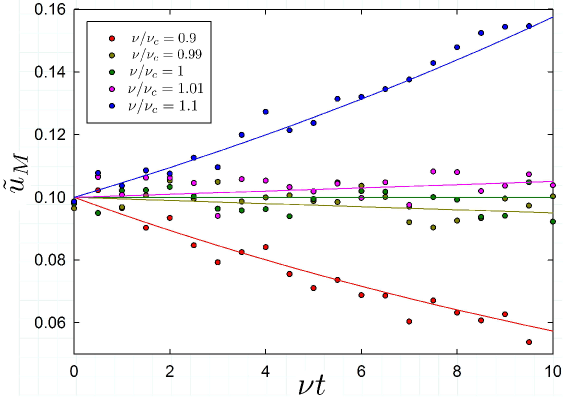
Figure 5: (Colour online) Rescaled velocity profile maximum $\tilde{u}_{M}=\tilde{u}(x_{M},t)$ as a function of time. Trajectories start from a sinusoidal average velocity profile $u(x,0)=u_{0}\sin(2\pi x)$, with $u_{0}=0.1$, which gives hydrodynamic predictions $\tilde{u}(x,t)=u_{0}\sin(2\pi x)e^{(\nu-\nu_{c})t/2}$ (then, $x_{M}=1/4$), drawn as solid lines. The system size is $N=500$ and we have averaged over $M=10^{5}$ trajectories.

6.3 Uniform Shear Flow state

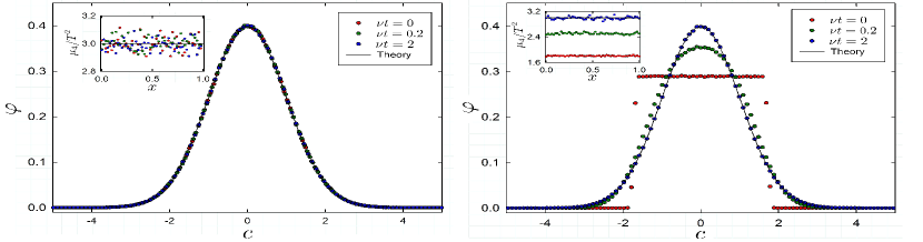
Figure 6: (Colour online) Evolution of the scaled one-particle velocity distribution, as given by (100), to the USF Gaussian steady distribution (70). In both panels, the initial velocity profile is the steady one $u_{s}(x)$ and the initial temperature is homogeneous, $T_{0}=1\neq T_{s}$, for a shear rate $a=5$ in a system with $N=500$ and $\nu=20$. The difference comes from the shape of the initial velocity distribution: Gaussian (left panel) vs. square (right panel). In the insets, we show the time evolution of the fourth central moment $\mu_{4}$ over $T^{2}$. Averages in both panels correspond to $M=10^{4}$ trajectories.

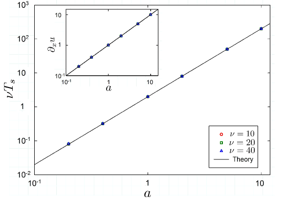
Figure 7: (Colour online) Steady temperature in the USF state as a function of the shear rate $a$. We consider three different values of $\nu$ in a system of size $N=500$, with averages over $M=10^{5}$ realisations. Specifically, we plot $\nu T_{s}$, the theoretical value of which is $2a^{2}$, as given by (67). In the inset, we show the numerical value of the velocity gradient $\partial_{x}u_{s}(x)$ as a function of the shear rate. Note the logarithmic scale in both axes.

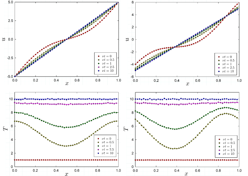
Figure 8: (Colour online) Transient evolution of the velocity (top) and the temperature (bottom) to their steady profiles in the USF state, for $a=10$. The numerical curves are plotted with points, whereas the solid lines correspond to the theoretical expression (76). The agreement between simulation and theory is excellent in both cases. The system size is $N=500$, the dissipation coefficient is $\nu=20$, and the number of trajectories is $M=10^{5}$.

The Uniform Shear Flow described in section 4.2 can be simulated by introducing appropriate boundary conditions in the simulations. When the pair $(1,N)$ is chosen to collide at time $p$, there are two separate collisions: particle $1$ ($N$) undergoes a collision with a particle with velocity $v_{N,p}-a$ ($v_{1,p}+a$). These boundary collision rules introduce a shear rate $a$ between the left and right ends of the system, and at the hydrodynamic level are represented by the Lees-Edwards conditions (66). This can be readily shown by considering the special evolution equations for $v_{1,p}$ and $v_{N,p}$ with the above boundary collision rules in the hydrodynamic limit.

Firstly, in figure 6, we check numerically the tendency of the system to approach the steady Gaussian one-particle velocity distribution of the USF state, given by (70). We do so in two cases: in the left panel, we start from a Gaussian distribution with the steady velocity profile but with an initial value of the temperature $T_{0}=1\neq T_{s}$. No time evolution is apparent in the scaled variables, since the distribution remains a Gaussian of unit variance for all times. In the right panel, our simulation starts from a square distribution. It is clearly observed that the Gaussian shape is approached as time increases. In the inset of both panels, we show the fourth central moment $\mu_{4}$ over $T^{2}$ for the same time instants, which also clearly show the tendency towards their Gaussian value.

For the longest time in figure 6, $\nu t=2$, the one-particle velocity distribution has already reached its predicted Gaussian shape. It is worth pointing out that this is so although the temperature is still $10$% below its steady value. This suggests the existence of a two-step approach to the steady state. In a first stage, the one-particle distribution function forgets its initial conditions and tends to a “normal” solution of the kinetic equation. Afterwards, it is moving over this “normal” solution that the system reaches the steady state. This resembles the so-called hydrodynamic $\beta$-state reported by Trizac et al. in a uniformly heated granular gas beta-state-1 ; beta-state-2 .

Secondly, we have tested our theoretical predictions in the USF state, given by (67), for the steady (i) profile of the average velocity and (ii) value of the temperature. We have done so in a system with $N=500$ and three different values of $\nu$, namely $\nu=10$, $20$ and $40$. As seen in figure 7, the agreement is excellent in all cases.

Finally, in figure 8, we check the tendency of the hydrodynamic variables $u$ and $T$ towards their USF values, whose theory was developed in section 4.2.1. In the left and right panels, we present the evolution of the velocity and temperature profiles towards its steady value from an initial state such that (i) $T(x,t=0)=T_{0}=1$ and (ii)

$$u(x,t=0)=u_{s}(x)+A\sin(2\pi x),\quad A=1,$$ (102)

$$u(x,t=0)=u_{s}(x)+A\sin(2\pi x)+B\cos(2\pi x),\quad A=B=1,$$ (103)

respectively. In both cases, there is only one Fourier mode: that corresponding to $n=1$. However, an important physical difference should be stressed: the temperature profile is always horizontal at the boundaries in the left panel, but it is not in the right one. Therefore, there is heat flux at the system boundaries in the latter case but not in the former. Anyhow, the agreement between simulation and theory is excellent in both situations.

6.4 The Couette flow state

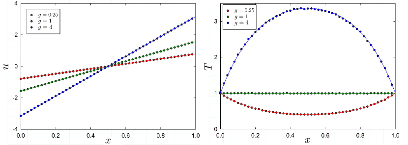
Figure 9: (Colour online) Numerical results (symbols) and theoretical values (solid lines) for the stationary velocity profile $u(x)$ (left) and the stationary temperature profile $T(x)$ (right) in the Couette state. The parameter values are $\nu=20$, $N=500$, $M=10^{5}$, and we have considered several values of $g$. The profiles have been plotted at the final time $\nu t=20$.

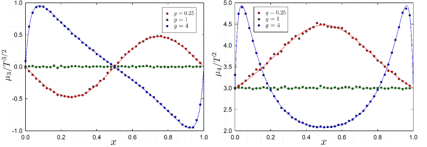
Figure 10: (Colour online) Third and fourth central moments $\mu_{3}$ and $\mu_{4}$ in the Couette steady state for the same simulation as in Fig. 9. Numerical results are shown with symbols whereas the lines stand for the theoretical prediction, i.e. the solutions of (50).

Now we consider a system coupled to two reservoirs at both ends, as described in section 4.3. In the simulations, two “extra” sites $0$ and $N+1$ are introduced, so that the number of colliding pairs is $L=N+1$. When the pair to collide involves one boundary particle (that is, pairs $(0,1)$ or $(N,N+1)$), the same collision rule for the bulk pairs $(1,2),\ldots,(N-1,N)$ is applied but the velocity of the “wall” particles is drawn from a Gaussian distribution with fixed average velocities $u_{L/R}$ and temperatures $T_{L/R}$. This is the only change in the simulations, which no longer correspond to periodic boundary conditions either in $u$ or $T$. In particular, the non-periodicity of $u^{\prime}$ implies that momentum is not conserved in the time evolution of the system, conversely to the case of the HCS and USF states.

In figure 9, we report the comparison between simulations and theoretical predictions from  (78), for different values of the parameter $g=2a^{2}/(\nu T_{B})$. The boundary conditions are chosen as $T_{L/R}=T_{B}=1$, $u_{R}=-u_{L}=a/2$. It should be recalled that $g=1$ corresponds to the case in which the Couette steady state coincides with the USF state and there is no heat current in the system. For $g>1$ ($g<1$), viscous heating is stronger (weaker) than that of the USF, and the steady temperature profile is concave (convex), that is, $T^{\prime\prime}<0$ ($T^{\prime\prime}>0$) and displays a maximum (minimum) at the centre of the system $x=1/2$. Simulations start from a non-stationary profile, initial particle velocities are drawn from a Gaussian distribution with local average velocity $u(x,0)=0$ and temperature $T(x,0)=1$. An excellent agreement is found in all the cases.

Figure 10 depicts the third and fourth central moments of the one-particle velocity distribution, scaled with their corresponding powers of the temperature, namely $\mu_{3}/T^{3/2}$ and $\mu_{4}/T^{2}$. Both moments display a non-trivial structure. In particular, the non-vanishing third moment clearly shows that the one-particle distribution is not symmetric with respect to the average velocity $u$. It is evident that the distribution is non-Gaussian, except for the case $T_{B}=2a^{2}/\nu$, which corresponds to the USF state.

6.5 Fluctuating currents

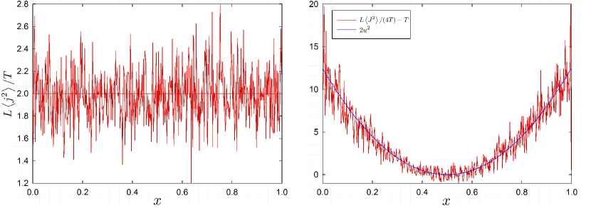
Figure 11: (Colour online) Left: Amplitude of the momentum current as a function of $x$ in the USF state. Specifically, we plot the rescaled amplitude $L\langle j^{2}(x,t)\rangle/T_{s}$ in the simulations (red line) and the theoretical value $2$ (black line). Right: Amplitude of the energy current as a function of $x$ in the USF state. Here, we plot $L\langle J^{2}(x,t)\rangle/4T(x,t)-T(x,t)$ as measured in the simulations (red line) and the numerical value of $2u_{s}^{2}(x)$ (blue line). All the simulations have been done in a system with $N=500$, $\nu=20$, $a=5$, and $M=10^{5}$.

A comparison for the amplitudes of noise for the velocity and energy currents is shown in Fig. 11. We carry it out in the USF state, in which the steady distribution is Gaussian but the average velocity is not homogeneous. This allows us to make a more exigent test of the theoretical result for the amplitude of the energy current, as given by (95), which contains a term proportional to $u^{2}$. The agreement is excellent for the amplitudes of both noises.

7 Conclusions

The $1d$ lattice model presented in this paper reproduces many of the physical states that are associated to the the shear mode of the velocity, i.e. the velocity component perpendicular to the gradient direction, of granular fluids. Specifically, we have been able to peruse the Homogeneous Cooling state together with its linear instability for large enough system sizes, and the stationary Uniform Shear Flow and Couette Flow states.

The simplicity of the model allows us to rigorously derive the hydrodynamic limit. Not only have we done this at the level of the evolution equation for the average velocity and temperature but also for the one-particle velocity distribution function. It must be noted that the energy dissipation at the hydrodynamic level is characterised by a finite cooling rate $\nu$, similarly to the case of granular gases. Though the underlying microscopic dynamics is quasi-elastic, the system is not “weakly dissipative” at the hydrodynamic level. Of course, a “weakly dissipative” regime may be considered by taking the limit $\nu\ll 1$, similarly to what was done in PLyH11a ; PLyH12a for a simpler model without momentum conservation. Also, we have also succeeded in writing down the fluctuating hydrodynamic description, for which the noises have been shown to be Gaussian and white.

The soundness of the hydrodynamic description developed in this paper is strongly supported by the numerical evidence. We have successfully compared our theoretical results with extensive Monte Carlo simulations of the model. In addition to the agreement found at the level of the average hydrodynamic variables, we have also obtained an excellent match at the level of the one-particle distribution function. The latter check has been done both directly, by computing the one-particle distribution in some physical situations, and indirectly, through higher moments thereof such as those appearing in the amplitude of the currents noises in the fluctuating hydrodynamics description.

An interesting result for our lattice model is the validity of the “Molecular Chaos” approximation, in the sense that the two-particle velocity distribution function factorise into the product of the corresponding one-particle distributions, apart from finite-size corrections. This is remarkable, since there is no mass transport in the system and particles always collide with their nearest neighbours, which on a physical basis seems to favour higher values of the correlations. In fact, the molecular chaos property is essential to have a closed hydrodynamic description, in which the evolution of the hydrodynamic fields, average velocity and temperature, are decoupled from that of the correlations over the hydrodynamic time scale.

Finite-size effects are expected to be important in granular gases. In many cases, we have minimised them in the present study by considering a specific value of the macroscopic cooling rate $\nu\simeq 2\pi^{2}$, for which we have previously shown noi that the finite-size effects coming from the nearest-neighbour correlation $\langle v_{i}v_{i+1}\rangle$ are as smallest as possible. Of course, finite-size effects are also relevant in the present model and, due to its simplicity, they can be investigated to a large extent. We defer this analysis to a later paper.

We have been able to derive analytically the shape of the one-particle distribution function for some physical states. Specifically, in both the HCS Gaussian_HCS and the USF state, the one-particle distribution function is Gaussian and therefore the amplitude of the current noises that appear in the fluctuating hydrodynamics description can be calculated. Interestingly, this paves the way for generalising Bertini’s et al. Macroscopic Fluctuation Theory to dissipative systems with conserved momentum and obtaining the large deviation function characterising the fluctuations of time-integrated quantities.

Our numerical simulations in the USF state suggest that the system approaches this steady state in a two-step process. First, initial conditions are forgotten and the one-particle distribution function reaches a “normal” solution. Second, the system approaches the steady state moving over this normal solution. This is utterly analogous to the existence of the so-called $\beta$-state in uniformly heated granular gases beta-state-1 ; beta-state-2 . Interestingly, the existence of this “normal” state is also related to the emergence of memory effects kovacs-granular-1 ; kovacs-granular-2 , which are worth investigating.

We have restricted ourselves throughout the paper to a velocity independent collision frequency ($\beta=0$), which is the analogous to the so-called Maxwell molecules model in kinetic theory. This is quite a natural choice in our case, since the velocities are perpendicular to the (possible) gradient direction. Nonetheless, other values of $\beta$ may be considered to tailor our model to fit the hydrodynamic equations for other relevant cases, such as hard-spheres. We have not analysed those in the present paper because the mathematical treatment is quite different and much more involved than that for MM. As is also the case in “real” granular gases when described starting from the Boltzmann equation, the hydrodynamic equations are not closed and constitutive equations are needed for the momentum and energy currents. Unfortunately, these constitutive equations cannot be inferred by using the local equilibrium approximation, which, unlike to the MM case, does not hold even for the simplest situations like the HCS and the USF states.

Our results differ from previous work in simple dissipative models in a remarkable point: contrarily to what was observed in PLyH12a ; PLyH13 , local equilibrium does not hold in general, even with the assumption of quasi-elastic microscopic dynamics considered in the hydrodynamic limit. Since the main physical difference between both models is the introduction here of a new conserved field (momentum), it is tempting to attribute this important difference to momentum conservation. Notwithstanding, we do not have a rigorous proof of this point, which indeed deserves further investigation.

Appendix: Gaussian character of the noises

In the large system size limit $L\gg 1$, the current noise introduced in the subsection (5.1) is white. We can introduce a new noise field $\tilde{\xi}(x,t)$ by

$$\xi^{(j)}(x,t)=L^{-1/2}\tilde{\xi}(x,t)$$ (104)

and $\tilde{\xi}(x,t)$ remains finite in the large system size limit $L\rightarrow\infty$,

$$\langle\tilde{\xi}(x,t)\rangle=0,\,\qquad\langle\tilde{\xi}(x,t)\tilde{\xi}(x^{\prime},t^{\prime})\rangle\sim 2\,T(x,t)\delta(x-x^{\prime})\delta(t-t^{\prime}).$$ (105)

Here we show that all the higher-order cumulants of $\tilde{\xi}(x,t)$ vanish in the thermodynamic limit as $L\rightarrow\infty$. Let us consider a cumulant of order $n$ of the microscopic noise $\xi_{l,p}$ that is equal to the $n$-th order moment of the $\xi$ plus a sum of nonlinear products of lower moments of $\xi$. A calculation analogous to the one carried out for the correlation $\langle\xi^{(j)}_{l,p}\xi^{(j)}_{l^{\prime},p^{\prime}}\rangle$ shows that the leading behaviour of any moment is of the order of $L^{-1}$, which is obtained when all the times are the same. Therefore, the moment $\langle j_{l,p}j_{l^{\prime},p^{\prime}}...j_{l^{(n)},p^{(n)}}\rangle$ gives the leading behaviour of the considered cumulant, which is thus of the order of $L^{-1}$ for $p=p^{\prime}=...=p^{(n)}$; any other contribution to the cumulant is at least of the order of $L^{-2}$. We have that

$$\langle j_{l,p}j_{l^{\prime},p^{\prime}}\cdots j_{l^{(n)},p^{(n)}}\rangle\sim L^{-1}\langle C_{l,p}\rangle\delta_{l,l^{\prime}}\delta_{l^{\prime},l^{\prime\prime}}\delta_{l^{(n-1)},l^{(n)}}\cdots\delta_{p,p^{\prime}}\delta_{p^{\prime},p^{\prime\prime}}\delta_{p^{(n-1)},p^{(n)}},$$ (106)

where $\langle C_{l,p}\rangle$ is certain average that remains finite in the large system size limit as $L\rightarrow\infty$. In the continuous limit, each current introduces a factor $L^{2}$ due to the scaling introduced in section 5. Moreover, we take into account the relationship (90) between Kronecker and Dirac $\delta$’s to write the cumulants $\langle\langle\cdots\rangle\rangle$ of the rescaled noise introduced in (104) as

$$\langle\langle\tilde{\xi}(x,t)\tilde{\xi}(x^{\prime},t^{\prime})\cdots\tilde{\xi}(x^{(n)},t^{(n)})\rangle\rangle\sim{L^{3\left(1-\frac{n}{2}\right)}}{\langle C(x,t)\rangle}\times$$

$$\qquad\delta(x-x^{\prime})\delta(x^{\prime}-x^{\prime\prime})\delta(x^{(n-1)}-x^{(n)})\cdots\delta(t-t^{\prime})\delta(t^{\prime}-t^{\prime\prime})\delta(t^{(n-1)}-t^{(n)}).$$

Thus, in the limit as $L\rightarrow\infty$,

$$\langle\tilde{\xi}(x,t)\tilde{\xi}(x^{\prime},t^{\prime})\cdots\tilde{\xi}(x^{(n)},t^{(n)})\rangle=0,\quad\textrm{for all $n>2$},$$ (108)

and the vanishing of all the cumulants for $n>2$ means that the momentum current noise is Gaussian in the infinite size limit.

The same procedure can be repeated for the energy current noise, by defining $\xi^{(J)}(x,t)=L^{-1/2}\tilde{\eta}(x,t)$), with the result

$$\langle\langle\tilde{\eta}(x,t)\tilde{\eta}(x^{\prime},t^{\prime})\cdots\tilde{\eta}(x^{(n)},t^{(n)})\rangle\rangle\sim{L^{3\left(1-\frac{n}{2}\right)}}{\langle D(x,t)\rangle}\times$$

$$\qquad\delta(x-x^{\prime})\delta(x^{\prime}-x^{\prime\prime})\delta(x^{(n-1)}-x^{(n)})\cdots\delta(t-t^{\prime})\delta(t^{\prime}-t^{\prime\prime})\delta(t^{(n-1)}-t^{(n)}).$$

In the equation above, $\langle D(x,t)\rangle$ is a certain average, different from $\langle C(x,t)\rangle$, but also finite in the large system size limit. Thus, we have that

$$\langle\tilde{\eta}(x,t)\tilde{\eta}(x^{\prime},t^{\prime})\cdots\tilde{\eta}(x^{n},t^{n})\rangle=0,\quad\textrm{for all $n>2$},$$ (110)

and the energy current noise also becomes Gaussian in the hydrodynamic limit.

Note that the Gaussianity of the noises is independent of the validity of the local equilibrium approximation, which is only needed to write $\langle C(x,t)\rangle$ and $\langle D(x,t)\rangle$ in terms of the hydrodynamic fields $u(x,t)$ and $T(x,t)$. Besides, a similar procedure for the dissipation noise gives that the corresponding scaled noise vanishes in the hydrodynamic limit, since the power of $L$ in the dominant contribution to the $n$-th order cumulant is $3-5n/2$ instead of $3-3n/2$. This means that the dissipation noise is subdominant as compared to the currents noises in the hydrodynamic limit, and can be neglected.

References

- (1) H. M. Jaeger, S. R. Nagel, and R. P. Behringer, “Granular solids, liquids, and gases,” Rev. Mod. Phys., vol. 68, no. 4, p. 1259, 1996.
- (2) A. Puglisi, Transport and fluctuations in granular fluids. Springer, Berlin, 2014.
- (3) N. Brilliantov and T. Pöschel, eds., Kinetic Theory of Granular Gases. Oxford University Press, 2004.
- (4) T. P. C. van Noije and M. H. Ernst, “Velocity distributions in homogeneous granular fluids: the free and the heated case,” Gran. Matt., vol. 1, p. 57, 1998.
- (5) C. K. K. Lun, S. B. Savage, D. J. Jeffrey, and N. Chepurniy, “Kinetic theories for granular flow: inelastic particles in couette flow and slightly inelastic particles in a general flowfield,” J. Fluid. Mech., vol. 140, p. 223, 1984.
- (6) J. J. Brey, J. W. Dufty, C. S. Kim, and A. Santos, “Hydrodynamics for granular flow at low density,” Phys. Rev. E, vol. 58, no. 4, p. 4638, 1998.
- (7) I. Goldhirsch, “Scales and kinetics of granular,” Chaos, vol. 9, p. 659, 1999.
- (8) L. P. Kadanoff, “Built upon sand: Theoretical ideas inspired by granular flows,” Rev. Mod. Phys., vol. 71, no. 1, pp. 435–444, 1999.
- (9) T. P. C. van Noije and M. H. Ernst, “Cahn-hilliard theory for unstable granular fluids,” Phys. Rev. E, vol. 61, p. 1765, 2000.
- (10) A. Einstein, “Zur allgemeinen molekularen theorie der wärme,” Ann. Phys., vol. 319, no. 7, pp. 354–362, 1904.
- (11) L. Onsager and S. Machlup, “Fluctuations and irreversible processes,” Phys. Rev., vol. 91, no. 6, p. 1505, 1953.
- (12) L. D. Landau and E. M. Lifshitz, Statistical Physics 3rd edition Course of Theoretical Physics Vol. 5. Pergamon Press. Oxford, 1980.
- (13) J. J. Brey, P. Maynar, and M. I. G. de Soria, “Fluctuating hydrodynamics for dilute granular gases,” Phys. Rev. E, vol. 79, p. 051305, 2009.
- (14) L. Bertini, A. De Sole, D. Gabrielli, G. Jona-Lasinio, and C. Landim, “Fluctuations in stationary nonequilibrium states of irreversible processes,” Phys. Rev. Lett., vol. 87, no. 4, p. 040601, 2001.
- (15) C. Kipnis and C. Landim, Scaling Limits of Interacting Particle Systems. Springer-Verlag, 1999.
- (16) C. Kipnis, C. Marchioro, and E. Presutti, “Heat flow in an exactly solvable model,” J. Stat. Phys., vol. 27, no. 1, pp. 65–74, 1982.
- (17) P. I. Hurtado and P. L. Garrido, “Test of the additivity principle for current fluctuations in a model of heat conduction,” Phys. Rev. Lett., vol. 102, no. 25, p. 250601, 2009.
- (18) P. I. Hurtado and P. L. Garrido, “Large fluctuations of the macroscopic current in diffusive systems: A numerical test of the additivity principle,” Phys. Rev. E, vol. 81, no. 4, p. 041102, 2010.
- (19) P. I. Hurtado and P. L. Garrido, “Current fluctuations and statistics during a large deviation event in an exactly solvable transport model,” J. Stat. Mech. (Theor. Exp.), vol. 2009, no. 02, p. P02032, 2009.
- (20) P. Hurtado and P. Krapivsky, “Compact waves in microscopic nonlinear diffusion,” Phys. Rev. E, vol. 85, no. 6, p. 060103, 2012.
- (21) A. Prados, A. Lasanta, and P. I. Hurtado, “Nonlinear driven diffusive systems with dissipation: Fluctuating hydrodynamics,” Phys. Rev. E, vol. 86, no. 3, p. 031134, 2012.
- (22) A. Prados, A. Lasanta, and P. I. Hurtado, “Large fluctuations in driven dissipative media,” Phys. Rev. Lett., vol. 107, no. 14, p. 140601, 2011.
- (23) P. I. Hurtado, A. Lasanta, and A. Prados, “Typical and rare fluctuations in nonlinear driven diffusive systems with dissipation,” Phys. Rev. E, vol. 88, no. 2, p. 022110, 2013.
- (24) A. Lasanta, A. Manacorda, A. Prados, and A. Puglisi, “Fluctuating hydrodynamics and mesoscopic effects of spatial correlations in dissipative systems with conserved momentum,” New J. Phys., vol. 17, p. 083039, 2015.
- (25) G. Grinstein, D.-H. Lee, and S. Sachdev, “Conservation laws, anisotropy, and “self-organized criticality”in noisy nonequilibrium systems,” Phys. Rev. Lett., vol. 64, no. 16, p. 1927, 1990.
- (26) P. L. Garrido, J. L. Lebowitz, C. Maes, and H. Spohn, “Long-range correlations for conservative dynamics,” Phys. Rev. A, vol. 42, no. 4, p. 1954, 1990.
- (27) S. Ramaswamy, “The mechanics and statistics of active matter,” Annu. Rev. Condens. Matter Phys., vol. 1, p. 323, 2010.
- (28) N. Kumar, H. Soni, S. Ramaswamy, and A. K. Sood, “Flocking at a distance in active granular matter,” Nature Communications, vol. 5, p. 4688, 2014.
- (29) A. Baskaran and M. C. Marchetti, “Enhanced diffusion and ordering of self-propelled rods,” Phys. Rev. Lett., vol. 101, p. 268101, 2008.
- (30) M. Marchetti, J. Joanny, S. Ramaswamy, T. Liverpool, J. Prost, M. Rao, and R. A. Simha, “Hydrodynamics of soft active matter,” Rev. Mod. Phys., vol. 85, no. 3, p. 1143, 2013.
- (31) H. Chaté, F. Ginelli, and R. Montagne, “Simple model for active nematics: Quasi-long-range order and giant fluctuations,” Phys. Rev. Lett., vol. 96, p. 180602, 2006.
- (32) J. R. Raymond and M. R. Evans, “Flocking regimes in a simple lattice model,” Phys. Rev. E, vol. 73, p. 036112, 2006.
- (33) R. A. Simha and S. Ramaswamy, “Hydrodynamic fluctuations and instabilities in ordered suspensions of self-propelled particles,” Phys. Rev. Lett., vol. 89, p. 058101, 2002.
- (34) J. J. Brey and D. Cubero, “Hydrodynamic transport coefficients of granular gases,” in Granular Gas (T. Pöschel and S. Luding, eds.), Springer (Berlin), 2001.
- (35) P. Haff, “Grain flow as a fluid-mechanical phenomenon,” J. Fluid Mech., vol. 134, pp. 401–430, 1983.
- (36) H. Ernst, “Nonlinear model-Boltzmann equations and exact solutions,” Phys. Rep., vol. 78, pp. 1–171, 1981.
- (37) J. J. Brey, M. Ruiz-Montero, and D. Cubero, “Homogeneous cooling state of a low-density granular flow,” Phys. Rev. E, vol. 54, no. 4, p. 3664, 1996.
- (38) J. J. Brey, A. Prados, M. G. de Soria, and P. Maynar, “Scaling and aging in the homogeneous cooling state of a granular fluid of hard particles,” Journal of Physics A: Mathematical and Theoretical, vol. 40, no. 48, p. 14331, 2007.
- (39) A. Baldassarri, U. M. B. Marconi, and A. Puglisi, “Influence of correlations on the velocity statistics of scalar granular gases,” EPL (Europhysics Letters), vol. 58, no. 1, p. 14, 2002.
- (40) A. Puglisi, V. Loreto, U. M. B. Marconi, and A. Vulpiani, “Clustering and non-gaussian behavior in granular matter,” Phys. Rev. Lett., vol. 81, p. 3848, 1998.
- (41) T. P. C. van Noije, M. H. Ernst, E. Trizac, and I. Pagonabarraga, “Randomly driven granular fluids: Large-scale structure,” Phys. Rev. E, vol. 59, p. 4326, 1999.
- (42) T. Pöschel and S. Luding, eds., Granular Gases. Lecture Notes in Physics vol. 564. Springer-Verlag, Berlin, 2001.
- (43) M. H. Ernst, E. Trizac, and A. Barrat, “The rich behavior of the boltzmann equation for dissipative gases,” Europhys. Lett., vol. 76, p. 56, 2006.
- (44) A. B. Bortz, M. H. Kalos, and J. L. Lebowitz, “A new algorithm for Monte Carlo simulation of Ising spin systems,” Journal of Computational Physics, vol. 17, no. 1, pp. 10–18, 1975.
- (45) A. Prados, J. J. Brey, and B. Sanchez-Rey, “A dynamical monte carlo algorithm for master equations with time-dependent transition rates,” Journal of statistical physics, vol. 89, no. 3-4, pp. 709–734, 1997.
- (46) N. G. V. Kampen, Stochastic Processes in Physics and Chemistry. Norht-Holland, Amsterdam, 1992.
- (47) U. M. B. Marconi, A. Puglisi, and A. Vulpiani, “About an h-theorem for systems with non-conservative interactions,” J. Stat. Mech., vol. 2013, p. P08003, 2013.
- (48) M. I. G. de Soria, P. Maynar, S. Mischler, C. Mouhot, T. Rey, and E. Trizac, “Towards an h-theorem for granular gases,” Journal of Statistical Mechanics: Theory and Experiment, vol. 2015, no. 11, p. P11009, 2015.
- (49) C. A. Plata, A. Manacorda, A. Lasanta, A. Puglisi, and A. Prados, “Lattice models for granular-like velocity fields: finite size effects.” (to be published).
- (50) S. McNamara, “Hydrodynamic modes of a uniform granular medium,” Physics of Fluids A, vol. 5, p. 3056, 1993.
- (51) T. P. C. van Noije, M. H. Ernst, R. Brito, and J. A. G. Orza, “Mesoscopic theory of granular fluids,” Phys. Rev. Lett., vol. 79, p. 411, 1997.
- (52) M. I. García de Soria, P. Maynar, G. Schehr, A. Barrat, and E. Trizac, “Dynamics of annihilation i. linearized boltzmann equation and hydrodynamics,” Phys. Rev. E, vol. 77, p. 051127, May 2008.
- (53) A. W. Lees and S. F. Edwards, “The computer study of transport processes under extreme conditions,” Journal of Physics C: Solid State Physics, vol. 5, no. 15, p. 1921, 1972.
- (54) A. Santos and V. Garzó, “Simple shear flow in inelastic maxwell models,” Journal of Statistical Mechanics: Theory and Experiment, vol. 2007, no. 08, p. P08021, 2007.
- (55) A. Santos, V. Garzó, and J. W. Dufty, “Inherent rheology of a granular fluid in uniform shear flow,” Phys. Rev. E, vol. 69, p. 061303, Jun 2004.
- (56) V. Garzó, “Transport coefficients for an inelastic gas around uniform shear flow: Linear stability analysis,” Phys. Rev. E, vol. 73, p. 021304, Feb 2006.
- (57) For the usual choice of an initial Gaussian distribution, see section 4.1.
- (58) M. I. García de Soria, P. Maynar, and E. Trizac, “Universal reference state in a driven homogeneous granular gas,” Phys. Rev. E, vol. 85, p. 051301, May 2012.
- (59) M. I. García de Soria, P. Maynar, and E. Trizac, “Linear hydrodynamics for driven granular gases,” Phys. Rev. E, vol. 87, p. 022201, Feb 2013.
- (60) A. Prados and E. Trizac, “Kovacs-like memory effect in driven granular gases,” Phys. Rev. Lett., vol. 112, p. 198001, May 2014.
- (61) E. Trizac and A. Prados, “Memory effect in uniformly heated granular gases,” Phys. Rev. E, vol. 90, p. 012204, Jul 2014.