Fully Computable Error Bounds for Eigenvalue Problem

Abstract

This paper is concerned with the computable error estimates for the eigenvalue problem which is solved by the general conforming finite element methods on the general meshes. Based on the computable error estimate, we can give an asymptotically lower bound of the general eigenvalues. Furthermore, we also give a guaranteed upper bound of the error estimates for the first eigenfunction approximation and a guaranteed lower bound of the first eigenvalue based on computable error estimator. Some numerical examples are presented to validate the theoretical results deduced in this paper.

Keywords. Eigenvalue problem, computable error estimate, guaranteed upper bound, guaranteed lower bound, complementary method.

AMS subject classifications. 65N30, 65N25, 65L15, 65B99.

1 Introduction

This paper is concerned with the computable error estimates for the eigenvalue problem by the finite element method. As we know, the priori error estimates can only give the asymptotic convergence order. The a posteriori error estimates are very important for the mesh adaption process. About the a posteriori error estimate for the partial differential equations by the finite element method, please refer to [2, 6, 7, 8, 26, 27, 31] and the references cited therein.

It is well known that the numerical approximations by the conforming finite element methods are upper bounds of the exact eigenvalues. Recently, how to obtain the lower bounds of the desired eigenvalues is a hot topic since it has many applications in some classical problems [3, 10, 11, 15, 17, 18, 21, 22, 23, 28, 34, 35]. So far, there have developed the nonconforming finite element methods, interpolation constant based methods and computational error estimate methods. The nonconforming finite element methods can only obtain the asymptotically lower bounds with the lowest order accuracy. The interpolation constant method can only obtain the efficient lowest order accuracy on the quasi-uniform meshes. The interesting computational error method need a condition that the numerical approximation is closer to the first eigenvalue than the second one. But the paper [28] gives a clue to us.

This paper is to give computable error estimates for the eigenpair approximations. We produce a guaranteed upper-bound error estimate for the first eigenfunction approximation and then a guaranteed lower bound of the first eigenvalue. The approach is based on complementary energy method from [14, 26, 27, 29, 30] coupled with the upper and lower bounds of the eigenvalues by the conforming and nonconforming finite element methods. The first eigenvalue is the key information in many practical applications such as Friedrichs, Poincaré, trace and similar inequalities (cf. [28]). Thus the two-sided bounds of the first eigenvalue of the partial differential operators are very important. Further, the proposed computable error estimates are asymptotically exact for the general eigenpair approximations which are obtained by the conforming finite element method. Based on this property, we can provide asymptotically lower bounds for general eigenvalues by the finite element method. The most important feature and contribution of this paper are that the method can also provide the reasonable accuracy even on the general regular meshes which is different from the existed methods.

An outline of the paper goes as follows. In Section 2, we introduce the finite element method for the eigenvalue problem and the corresponding basic error estimates. The computable error estimates for the eigenfunction approximations and the corresponding upper-bound properties are given in Section 3. In Section 4, lower bounds of eigenvalues are obtained based on the results in Section 3. Some numerical examples are presented to validate our theoretical analysis in Section 5. Some concluding remarks are given in the last section.

2 Finite element method for eigenvalue problem

This section is devoted to introducing some notation and the finite element method for eigenvalue problem. In this paper, the standard notation for Sobolev spaces $H^{s}(\Omega)$ and $H({\rm div};\Omega)$ and their associated norms and semi-norms [1] will be used. We denote $H_{0}^{1}(\Omega)=\{v\in H^{1}(\Omega):\ v|_{\partial\Omega}=0\}$, where $v|_{\partial\Omega}=0$ is in the sense of trace. The letter $C$ (with or without subscripts) denotes a generic positive constant which may be different at its different occurrences in the paper.

For simplicity, this paper is concerned with the following model problem: Find $(\lambda,u)$ such that

$$\left\{\begin{array}[]{rcl}-\Delta u+u&=&\lambda u,\quad{\rm in}\ \Omega,\\ u&=&0,\ \ \quad{\rm on}\ \partial\Omega,\end{array}\right.$$ (2.1)

where $\Omega\subset\mathcal{R}^{d}$ $(d=2,3)$ is a bounded domain with Lipschitz boundary $\partial\Omega$ and $\Delta$ denotes the Laplacian operator. We will find that the method in this paper can easily be extended to more general eigenvalue problems.

In order to use the finite element method to solve the eigenvalue problem (2.1), we need to define the corresponding variational form as follows: Find $(\lambda,u)\in\mathcal{R}\times V$ such that

$$a(u,v) = \lambda b(u,v),\quad\forall v\in V,$$ (2.2)

where $V:=H_{0}^{1}(\Omega)$ and

$$a(u,v)=\int_{\Omega}\big{(}\nabla u\cdot\nabla v+uv\big{)}d\Omega,\ \ \ \ \ \ b(u,v)=\int_{\Omega}uvd\Omega.$$ (2.3)

The norms $\|\cdot\|_{a}$ and $\|\cdot\|_{b}$ are defined by

$$\|v\|_{a}=\sqrt{a(v,v)}\ \ \ \ \ {\rm and}\ \ \ \ \ \|v\|_{b}=\sqrt{b(v,v)}.$$

It is well known that the eigenvalue problem (2.2) has an eigenvalue sequence $\{\lambda_{j}\}$ (cf. [5, 12]):

$$0<\lambda_{1}<\lambda_{2}\leq\cdots\leq\lambda_{k}\leq\cdots,\ \ \ \lim_{k\rightarrow\infty}\lambda_{k}=\infty,$$

and associated eigenfunctions

$$u_{1},u_{2},\cdots,u_{k},\cdots,$$

where $b(u_{i},u_{j})=0$ when $i\neq j$. The first eigenvalue $\lambda_{1}$ is simple and in the sequence $\{\lambda_{j}\}$, the $\lambda_{j}$ are repeated according to their geometric multiplicity.

Now, we introduce the finite element method for the eigenvalue problem (2.2). First we decompose the computing domain $\Omega\subset\mathcal{R}^{d}\ (d=2,3)$ into shape-regular triangles or rectangles for $d=2$ (tetrahedrons or hexahedrons for $d=3$) to produce the mesh $\mathcal{T}_{h}$ (cf. [8, 13]). In this paper, we use $\mathcal{E}_{h}$ to denote the set of interior faces (edges or sides) of $\mathcal{T}_{h}$. The diameter of a cell $K\in\mathcal{T}_{h}$ is denoted by $h_{K}$ and the mesh size $h$ describes the maximum diameter of all cells $K\in\mathcal{T}_{h}$. Based on the mesh $\mathcal{T}_{h}$, we can construct a finite element space denoted by $V_{h}\subset V$. For simplicity, we only consider the Lagrange type conforming finite element space which is defined as follows

$$V_{h}=\big{\{}v_{h}\in C(\Omega)\ \big{|}\ v_{h}|_{K}\in\mathcal{P}_{k},\ \ \forall K\in\mathcal{T}_{h}\big{\}}\cap H_{0}^{1}(\Omega),$$ (2.4)

where $\mathcal{P}_{k}$ denotes the space of polynomials of degree at most $k$.

We define the standard finite element scheme for the eigenvalue problem (2.2) as follows: Find $(\lambda_{h},u_{h})\in\mathcal{R}\times V_{h}$ such that $b(u_{h},u_{h})=1$ and

$$a(u_{h},v_{h}) = \lambda_{h}b(u_{h},v_{h}),\quad\ \ \ \forall v_{h}\in V_{h}.$$ (2.5)

From [4, 5, 12], the discrete eigenvalue problem (2.5) has eigenvalues:

$$0<\lambda_{1,h}<\lambda_{2,h}\leq\cdots\leq\lambda_{k,h}\leq\cdots\leq\lambda_{N_{h},h},$$

and corresponding eigenfunctions

$$u_{1,h},\cdots,u_{k,h},\cdots,u_{N_{h},h},$$

where $b(u_{i,h},u_{j,h})=\delta_{ij}$ ($\delta_{ij}$ denotes the Kronecker function), when $1\leq i,j\leq N_{h}$ ($N_{h}$ is the dimension of the finite element space $V_{h}$).

Let $M(\lambda_{i})$ denote the eigenspace corresponding to the eigenvalue $\lambda_{i}$ which is defined by

$$M(\lambda_{i}) = \big{\{}w\in H_{0}^{1}(\Omega):w\ {\rm is\ an\ eigenfunction\ of\ (\ref{weak_eigenvalue_problem})}$$

$$\ \ \ \ \ \ \ \ \ \ \ \ \ \ \ \ {\rm corresponding\ to}\ \lambda_{i}\big{\}},$$

and define

$$\delta_{h}(\lambda_{i})=\sup_{w\in M(\lambda_{i}),\|w\|_{b}=1}\inf_{v_{h}\in V_{h}}\|w-v_{h}\|_{a}.$$ (2.6)

We also define the following quantity:

$$\eta_{a}(h) = \sup_{f\in L^{2}(\Omega),\|f\|_{b}=1}\inf_{v_{h}\in V_{h}}\|Tf-v_{h}\|_{a},$$ (2.7)

where $T:L^{2}(\Omega)\rightarrow V$ is defined as

$$a(Tf,v)=b(f,v),\ \ \ \ \ \forall f\in L^{2}(\Omega)\ \ \ {\rm and}\ \ \ \forall v\in V.$$ (2.8)

Then the error estimates for the eigenpair approximations by the finite element method can be described as follows.

Lemma 2.1.

([4, Lemma 3.6, Theorem 4.4] and [12]) There exists the exact eigenpair $(\lambda_{i},u_{i})$ of (2.2) such that each eigenpair approximation $(\lambda_{i,h},u_{i,h})$ $(i=1,2,\cdots,N_{h})$ of (2.5) has the following error estimates

$$\|u_{i}-u_{i,h}\|_{a} \leq \big{(}1+C_{i}\eta_{a}(h)\big{)}\delta_{h}(\lambda_{i}),$$ (2.9)

$$\|u_{i}-u_{i,h}\|_{b} \leq C_{i}\eta_{a}(h)\|u_{i}-u_{i,h}\|_{a},$$ (2.10)

$$|\lambda_{i}-\lambda_{i,h}| \leq C_{i}\|u_{i}-u_{i,h}\|_{a}^{2}\leq C_{i}\eta_{a}(h)\|u_{i}-u_{i,h}\|_{a}.$$ (2.11)

Here and hereafter $C_{i}$ is some constant depending on $i$ but independent of the mesh size $h$.

3 Complementarity based error estimate

In this section, we derive a computable error estimate for the eigenfunction approximations based on complementarity approach. A guaranteed upper bound of the error estimate for the first eigenfunction approximation is designed based on the lower bounds of the second eigenvalue. We also produce an asymptotically upper bound error estimate for the general eigenfunction approximations which are obtained by solving the discrete eigenvalue problem (2.5).

First, we recall the following divergence theorem

$$\int_{\Omega}v{\rm div}\mathbf{z}d\Omega+\int_{\Omega}\mathbf{z}\cdot\nabla vd\Omega=\int_{\partial\Omega}v\mathbf{z}\cdot\nu ds,\ \ \ \forall v\in V,\ \forall\mathbf{z}\in\mathbf{W},$$ (3.1)

where $\mathbf{W}:=H({\rm div};\Omega)$ and $\nu$ denotes the unit outward normal to $\partial\Omega$.

We first give a guaranteed upper bound of the error estimate for the first eigenfunction approximation and the method used here is independent from the way to obtain the solution. We only consider the eigenfunction approximation $\widehat{u}_{1}\in V$ and estimate the error $e=u_{1}-\widehat{u}_{1}$ no matter how to obtain $\widehat{u}_{1}$. In this paper, we let $b(\widehat{u}_{1},\widehat{u}_{1})=1$ and the eigenvalue approximation $\widehat{\lambda}_{1}$ is determined as follows

$$\widehat{\lambda}_{1}=\frac{a(\widehat{u}_{1},\widehat{u}_{1})}{b(\widehat{u}_{1},\widehat{u}_{1})}=a(\widehat{u}_{1},\widehat{u}_{1}).$$

Theorem 3.1.

Assume we have an eigenpair approximation $(\widehat{\lambda}_{1},\widehat{u}_{1})\in\mathcal{R}\times V$ corresponding to the first eigenvalue $\lambda_{1}$ and a lower bound eigenvalue approximation $\lambda_{2}^{L}$ of the second eigenvalue $\lambda_{2}$ such that $\lambda_{1}\leq\widehat{\lambda}_{1}<\lambda_{2}^{L}\leq\lambda_{2}$. There exists an exact eigenfunction $u_{1}\in M(\lambda_{1})$ such that the error estimate for the first eigenfunction approximation $\widehat{u}_{1}\in V$ with $b(\widehat{u}_{1},\widehat{u}_{1})=1$ has the following guaranteed upper bound

$$\|u_{1}-\widehat{u}_{1}\|_{a} \leq \frac{\lambda_{2}^{L}}{\lambda_{2}^{L}-\widehat{\lambda}_{1}}\eta(\widehat{\lambda}_{1},\widehat{u}_{1},\mathbf{y}),\ \ \ \forall\mathbf{y}\in\mathbf{W},$$ (3.2)

where $\eta(\widehat{\lambda}_{1},\widehat{u}_{1},\mathbf{y})$ is defined as follows

$$\eta(\widehat{\lambda}_{1},\widehat{u}_{1},\mathbf{y}):=\big{(}\|\widehat{\lambda}_{1}\widehat{u}_{1}-\widehat{u}_{1}+{\rm div}\mathbf{y}\|_{0}^{2}+\|\mathbf{y}-\nabla\widehat{u}_{1}\|_{0}^{2}\big{)}^{1/2}.$$ (3.3)

Proof.

We can choose $u_{1}\in M(\lambda_{1})$ such that $b(v,u_{1}-\widehat{u}_{1})=0$ for any $v\in M(\lambda_{1})$. Now we set $w=u_{1}-\widehat{u}_{1}$ and the following estimates hold

$$a(u_{1}-\widehat{u}_{1},w)-\widehat{\lambda}_{1}b(u_{1}-\widehat{u}_{1},w)$$ (3.4)

$$= \int_{\Omega}\lambda_{1}u_{1}wd\Omega-\int_{\Omega}\nabla\widehat{u}_{1}\cdot\nabla wd\Omega-\int_{\Omega}\widehat{u}_{1}wd\Omega-\widehat{\lambda}_{1}\int_{\Omega}u_{1}wd\Omega$$

$$\ \ +\widehat{\lambda}_{1}\int_{\Omega}\widehat{u}_{1}wd\Omega+\int_{\Omega}w{\rm div}\mathbf{y}d\Omega+\int_{\Omega}\mathbf{y}\cdot\nabla wd\Omega$$

$$= \int_{\Omega}\big{(}\widehat{\lambda}_{1}\widehat{u}_{1}-\widehat{u}_{1}+{\rm div}\mathbf{y}\big{)}wd\Omega+\int_{\Omega}\big{(}\mathbf{y}-\nabla\widehat{u}_{1}\big{)}\cdot\nabla wd\Omega$$

$$\leq \|\widehat{\lambda}_{1}\widehat{u}_{1}-\widehat{u}_{1}+{\rm div}\mathbf{y}\|_{0}\|w\|_{0}+\|\mathbf{y}-\nabla\widehat{u}_{1}\|_{0}\|\nabla w\|_{0}$$

$$\leq \big{(}\|\widehat{\lambda}_{1}\widehat{u}_{1}-\widehat{u}_{1}+{\rm div}\mathbf{y}\|_{0}^{2}+\|\mathbf{y}-\nabla\widehat{u}_{1}\|_{0}^{2}\big{)}^{1/2}\|w\|_{a},\ \ \ \forall\mathbf{y}\in\mathbf{W}.$$

Since $b(v,u_{1}-\widehat{u}_{1})=0$ for any $v\in M(\lambda_{1})$, the following inequalities hold

$$\frac{\|w\|_{a}^{2}}{\|w\|_{b}^{2}}\geq\lambda_{2}\geq\lambda_{2}^{L}.$$ (3.5)

Combining (3.4) and (3.5) leads to the following estimate

$$\Big{(}1-\frac{\widehat{\lambda}_{1}}{\lambda_{2}^{L}}\Big{)}\|w\|_{a}^{2} \leq \eta(\widehat{\lambda}_{1},\widehat{u}_{1},\mathbf{y})\|w\|_{a},\ \ \ \forall\mathbf{y}\in\mathbf{W}.$$

It means that we have

$$\|w\|_{a} \leq \frac{\lambda_{2}^{L}}{\lambda_{2}^{L}-\widehat{\lambda}_{1}}\eta(\widehat{\lambda}_{1},\widehat{u}_{1},\mathbf{y}),\ \ \ \forall\mathbf{y}\in\mathbf{W}.$$

This is the desired result (3.2) and the proof is complete. ∎

A natural problem is to seek the minimization $\eta(\widehat{\lambda},\widehat{u},\mathbf{y})$ over $\mathbf{W}$ for the fixed eigenpair approximation $(\widehat{\lambda},\widehat{u})$. For this aim, we define the minimization problem: Find $\mathbf{y}^{*}\in\mathbf{W}$ such that

$$\eta(\widehat{\lambda},\widehat{u},\mathbf{y}^{*})\leq\eta(\widehat{\lambda},\widehat{u},\mathbf{y}),\ \ \ \ \forall\mathbf{y}\in\mathbf{W}.$$ (3.6)

From [29, 30], the optimization problem is equivalent to the following partial differential equation: Find $\mathbf{y}^{*}\in\mathbf{W}$ such that

$$a^{*}(\mathbf{y}^{*},\mathbf{z}) = \mathcal{F}^{*}(\widehat{\lambda},\widehat{u},\mathbf{z}),\ \ \ \ \forall\mathbf{z}\in\mathbf{W},$$ (3.7)

where

$$a^{*}(\mathbf{y}^{*},\mathbf{z})=\int_{\Omega}\big{(}{\rm div}\mathbf{y}^{*}{\rm div}\mathbf{z}+\mathbf{y}^{*}\cdot\mathbf{z}\big{)}d\Omega,\ \ \ \mathcal{F}^{*}(\widehat{\lambda},\widehat{u},\mathbf{z})=-\int_{\Omega}\widehat{\lambda}\widehat{u}{\rm div}\mathbf{z}d\Omega.$$

It is obvious $a^{*}(\cdot,\cdot)$ is an inner product in the space $\mathbf{W}$ and the corresponding norm is $\||\mathbf{z}\||_{*}=\sqrt{a^{*}(\mathbf{z},\mathbf{z})}$. From the Riesz theorem, we can know the dual problem (3.7) has a unique solution.

Now, we state some properties for the estimator $\eta(\widehat{\lambda},\widehat{u},\mathbf{y})$.

Lemma 3.1.

Assume $\mathbf{y}^{*}$ be the solution of the dual problem (3.7) and let $\widehat{\lambda}\in\mathcal{R}$, $\widehat{u}\in V$ and $\mathbf{y}\in\mathbf{W}$ be arbitrary. Then the following equality holds

$$\eta^{2}(\widehat{\lambda},\widehat{u},\mathbf{y}) = \eta^{2}(\widehat{\lambda},\widehat{u},\mathbf{y}^{*})+\||\mathbf{y}^{*}-\mathbf{y}\||_{*}^{2}.$$ (3.8)

In order to give a computable error estimate, the reasonable choice is a certain approximate solution $\mathbf{y}_{h}\in\mathbf{W}$ of the dual problem (3.7). Then we can give a guaranteed upper bound of the error estimate for the first eigenfunction approximation.

Corollary 3.1.

Under the conditions of Theorem 3.1, there exists an exact eigenfunction $u_{1}\in M(\lambda_{1})$ such that the error estimate for the eigenpair approximation $(\widehat{\lambda}_{1},\widehat{u}_{1})$ has the following upper bound

$$\|u_{1}-\widehat{u}_{1}\|_{a} \leq \frac{\lambda_{2}^{L}}{\lambda_{2}^{L}-\widehat{\lambda}_{1}}\eta(\widehat{\lambda}_{1},\widehat{u}_{1},\mathbf{y}_{h}),$$ (3.9)

where $\mathbf{y}_{h}\in\mathbf{W}$ is a reasonable approximate solution of the dual problem (3.7) with $\widehat{\lambda}=\widehat{\lambda}_{1}$ and $\widehat{u}=\widehat{u}_{1}$.

We would like to point out that the quantity $\eta(\lambda_{i,h},u_{i,h},\mathbf{y}^{*})$, where $\mathbf{y}^{*}\in\mathbf{W}$ is the solution of (3.7) with $\widehat{\lambda}=\lambda_{i,h}$ and $\widehat{u}=u_{i,h}$, is an asymptotically exact error estimate for the eigenfunction approximation $u_{i,h}$ when the eigenpair approximation is obtained by solving the discrete eigenvalue problem (2.5). Now, let us discuss the efficiency of the a posteriori error estimate $\eta(\lambda_{i,h},u_{i,h},\mathbf{y}^{*})$ and $\eta(\lambda_{i,h},u_{i,h},\mathbf{y}_{h})$.

Theorem 3.2.

Assume $(\lambda_{i,h},u_{i,h})$ be an eigenpair approximation of the discrete eigenvalue problem (2.5) corresponding to the eigenvalue $\lambda_{i}$. Then there exists an exact eigenfunction $u_{i}\in M(\lambda_{i})$ such that $\eta(\lambda_{i,h},u_{i,h},\mathbf{y}^{*})$ has the following inequalities

$$\theta_{1,i}\|u_{i}-u_{i,h}\|_{a}\leq\eta(\lambda_{i,h},u_{i,h},\mathbf{y}^{*})\leq\theta_{2,i}\|u_{i}-u_{i,h}\|_{a},$$ (3.10)

where $\mathbf{y}^{*}\in\mathbf{W}$ is the solution of the dual problem (3.7) with $\widehat{\lambda}=\lambda_{i,h}$ and $\widehat{u}=u_{i,h}$ and

$$\theta_{1,i}:=(1-C_{i}^{2}\lambda_{i,h}\eta_{a}^{2}(h))\ \ \ {\rm and}\ \ \ \theta_{2,i}:=\sqrt{1+\big{(}2(\lambda_{i}-1)^{2}+1\big{)}C_{i}^{2}\eta_{a}^{2}(h)}.$$ (3.11)

Further, we have the following asymptotic exactness

$$\lim_{h\rightarrow 0}\frac{\eta(\lambda_{i,h},u_{i,h},\mathbf{y}^{*})}{\|u_{i}-u_{i,h}\|_{a}}=1.$$ (3.12)

Proof.

Similarly, we can also choose $u_{i}\in M(\lambda_{i})$ such that $b(v,u_{i}-u_{i,h})=0$ for any $v\in M(\lambda_{i})$. Then from the similar process in (3.4), we have

$$\|u_{i}-u_{i,h}\|_{a}^{2}\leq\eta(\lambda_{i,h},u_{i,h},\mathbf{y})\|u_{i}-u_{i,h}\|_{a}+\lambda_{i,h}\|u_{i}-u_{i,h}\|_{b}^{2}$$

$$\leq\eta(\lambda_{i,h},u_{i,h},\mathbf{y})\|u_{i}-u_{i,h}\|_{a}+C_{i}^{2}\lambda_{i,h}\eta_{a}^{2}(h)\|u_{i}-u_{i,h}\|_{a}^{2},\ \ \ \forall\mathbf{y}\in\mathbf{W}.$$ (3.13)

It leads to

$$\|u_{i}-u_{i,h}\|_{a} \leq \frac{1}{1-C_{i}^{2}\lambda_{i,h}\eta_{a}^{2}(h)}\eta(\lambda_{i,h},u_{i,h},\mathbf{y}),\ \ \ \forall\mathbf{y}\in\mathbf{W}.$$ (3.14)

From the definition (3.3), the eigenvalue problem (2.1) and $\nabla u_{i}\in\mathbf{W}$, we have

$$\eta^{2}(\lambda_{i,h},u_{i,h},\nabla u_{i})=\|\nabla u_{i,h}-\nabla u_{i}\|_{b}^{2}+\|(\lambda_{i,h}-1)u_{i,h}-(\lambda_{i}-1)u_{i}\|_{b}^{2}.$$ (3.15)

Then combining (3.8), (3.15) and Lemma 2.1, the following estimates hold

$$\eta^{2}(\lambda_{i,h},u_{i,h},\mathbf{y}^{*})\leq\eta^{2}(\lambda_{i,h},u_{i,h},\nabla u_{i})$$ (3.16)

$$= \|\nabla u_{i,h}-\nabla u_{i}\|_{b}^{2}+\|(\lambda_{i,h}-1)u_{i,h}-(\lambda_{i}-1)u_{i}\|_{b}^{2}$$

$$= \|u_{i}-u_{i,h}\|_{a}^{2}+\|(\lambda_{i,h}-1)u_{i,h}-(\lambda_{i}-1)u_{i}\|_{b}^{2}-\|u_{i}-u_{i,h}\|_{b}^{2}$$

$$= \|u_{i}-u_{i,h}\|_{a}^{2}+\|(\lambda_{i,h}-\lambda_{i})u_{i,h}+(\lambda_{i}-1)(u_{i,h}-u_{i})\|_{b}^{2}-\|u_{i}-u_{i,h}\|_{b}^{2}$$

$$\leq \|u_{i}-u_{i,h}\|_{a}^{2}+2|\lambda_{i,h}-\lambda_{i}|^{2}+\big{(}2(\lambda_{i}-1)^{2}-1\big{)}\|u_{i}-u_{i,h}\|_{b}^{2}$$

$$\leq \big{(}1+2C_{i}^{2}\eta_{a}^{2}(h)+\big{(}2(\lambda_{i}-1)^{2}-1\big{)}C_{i}^{2}\eta_{a}^{2}(h)\big{)}\|u_{i}-u_{i,h}\|_{a}^{2}$$

$$\leq \big{(}1+\big{(}2(\lambda_{i}-1)^{2}+1\big{)}C_{i}^{2}\eta_{a}^{2}(h)\big{)}\|u_{i}-u_{i,h}\|_{a}^{2},$$

where we used the estimate

$$\lambda_{i,h}-\lambda_{i} \leq C_{i}\eta_{a}(h)\|u_{i}-u_{i,h}\|_{a}.$$

The inequality (3.16) leads to the following estimate

$$\eta(\lambda_{i,h},u_{i,h},\mathbf{y}^{*}) \leq \sqrt{1+\big{(}2(\lambda_{i}-1)^{2}+1\big{)}C_{i}^{2}\eta_{a}^{2}(h)}\|u_{i}-u_{i,h}\|_{a}.$$ (3.17)

From inequalities (3.8), (3.14) and (3.17), we obtain the desired result (3.10) and (3.12) can be deduced easily from the fact that $\eta_{a}(h)\rightarrow 0$ as $h\rightarrow 0$. ∎

Corollary 3.2.

Assume the conditions of Theorem 3.2 hold and there exists a constant $\gamma_{i}>0$ such that the approximation $\mathbf{y}_{h}$ of $\mathbf{y}^{*}$ satisfies $\||\mathbf{y}^{*}-\mathbf{y}_{h}\||_{*}\leq\gamma_{i}\|u_{i}-u_{i,h}\|_{a}$. Then the following efficiency holds

$$\eta(\lambda_{i,h},u_{i,h},\mathbf{y}_{h}) \leq \sqrt{\theta_{2,i}^{2}+\gamma_{i}^{2}}\|u_{i}-u_{i,h}\|_{a}.$$ (3.18)

Further, the estimator $\eta(\lambda_{i,h},u_{i,h},\mathbf{y}_{h})$ is asymptotically exact if and only if the following condition holds

$$\lim_{h\rightarrow 0}\frac{\||\mathbf{y}^{*}-\mathbf{y}_{h}\||_{*}}{\|u_{i}-u_{i,h}\|_{a}}=0.$$ (3.19)

Proof.

First from (3.8) and (3.10), we have

$$\eta^{2}(\lambda_{i,h},u_{i,h},\mathbf{y}_{h}) = \eta^{2}(\lambda_{i,h},u_{i,h},\mathbf{y}^{*})+\||\mathbf{y}^{*}-\mathbf{y}_{h}\||_{*}^{2}$$ (3.20)

$$\leq \theta_{2,i}^{2}\|u_{i}-u_{i,h}\|_{a}^{2}+\gamma_{i}^{2}\|u_{i}-u_{i,h}\|_{a}^{2}$$

$$\leq (\theta_{2,i}^{2}+\gamma_{i}^{2})\|u_{i}-u_{i,h}\|_{a}^{2}.$$

Then the desired result (3.18) can be obtained and the asymptotically exactness of the estimator follows immediately from the condition (3.19). ∎

4 Lower bound of the eigenvalue

In this section, based on the guaranteed upper bound for the error estimate of the first eigenfunction approximation, we give a guaranteed lower bound of the first eigenvalue. Further, we also give asymptotically lower bounds of the general eigenvalues based on the asymptotically exact error estimates for the general eigenfunction approximations which are obtained by solving the discrete finite element eigenvalue problem (2.5). Actually, the process is very direct since we have the following Rayleigh quotient expansion which comes from [4, 5].

Lemma 4.1.

([4, 5]) Assume $(\lambda,u)$ is an exact solution of the eigenvalue problem (2.2) and $0\neq\psi\in V$. Let us define

$$\bar{\lambda}=\frac{a(\psi,\psi)}{b(\psi,\psi)}.$$ (4.1)

Then we have

$$\bar{\lambda}-\lambda = \frac{a(u-\psi,u-\psi)}{b(\psi,\psi)}-\lambda\frac{b(u-\psi,u-\psi)}{b(\psi,\psi)}.$$ (4.2)

Theorem 4.1.

Assume $\lambda_{1}$ is the first eigenvalue of the eigenvalue problem (2.1) and $(\widehat{\lambda}_{1},\widehat{u}_{1})\in\mathcal{R}\times V$ ($\|\widehat{u}_{1}\|_{b}=1$) be the eigenpair approximation for the first eigenvalue and eigenfunction, respectively. Then we have the following guaranteed lower bound of the first eigenvalue

$$\widehat{\lambda}_{1}-\lambda_{1} \leq \left(\frac{\lambda_{2}^{L}}{\lambda_{2}^{L}-\widehat{\lambda}_{1}}\right)\frac{\lambda_{2}^{L}}{\lambda_{2}^{L}-\alpha^{2}\eta^{2}(\widehat{\lambda}_{1},\widehat{u}_{1},\mathbf{y}_{h})}\eta^{2}(\widehat{\lambda}_{1},\widehat{u}_{1},\mathbf{y}_{h}),$$ (4.3)

where $\alpha=\lambda_{2}^{L}/(\lambda_{2}^{L}-\widehat{\lambda}_{1})$ and $\mathbf{y}_{h}\in\mathbf{W}$ is a reasonable approximate solution of the dual problem (3.7) with $\widehat{\lambda}=\widehat{\lambda}_{1}$ and $\widehat{u}=\widehat{u}_{1}$.

Then the following guaranteed lower-bound result holds

$$\widehat{\lambda}_{1}^{L}:=\widehat{\lambda}_{1}-\left(\frac{\lambda_{2}^{L}}{\lambda_{2}^{L}-\widehat{\lambda}_{1}}\right)\frac{\lambda_{2}^{L}}{\lambda_{2}^{L}-\alpha^{2}\eta^{2}(\widehat{\lambda}_{1},\widehat{u}_{1},\mathbf{y}_{h})}\eta^{2}(\widehat{\lambda}_{1},\widehat{u}_{1},\mathbf{y}_{h})\leq\lambda_{1},$$ (4.4)

where $\widehat{\lambda}_{1}^{L}$ denotes a lower bound of the first eigenvalue $\lambda_{1}$.

Proof.

Similarly, we can also choose $u_{1}\in M(\lambda_{1})$ such that $b(v,u_{1}-\widehat{u}_{1})=0$ for any $v\in M(\lambda_{1})$. We also set $w=u_{1}-\widehat{u}_{1}$ and from Lemma 4.1, (3.2), (3.4) and $\|\widehat{u}_{1}\|_{b}=1$, we have

$$\widehat{\lambda}_{1}-\lambda_{1}-(\widehat{\lambda}_{1}-\lambda_{1})\|w\|_{b}^{2} = a(u_{1}-\widehat{u}_{1},u_{1}-\widehat{u}_{1})-\widehat{\lambda}_{1}b(u_{1}-\widehat{u}_{1},u_{1}-\widehat{u}_{1})$$ (4.5)

$$\leq \eta(\widehat{\lambda}_{1},\widehat{u}_{1},\mathbf{y}_{h})\|u_{1}-\widehat{u}_{1}\|_{a}.$$

Combining (3.2), (3.5) and (4.5) leads to the following inequalities

$$\widehat{\lambda}_{1}-\lambda_{1} \leq \frac{\|w\|_{a}}{1-\|w\|_{b}^{2}}\eta(\widehat{\lambda}_{1},\widehat{u}_{1},\mathbf{y}_{h})$$ (4.6)

$$\leq \frac{\|w\|_{a}}{1-\frac{1}{\lambda_{2}^{L}}\|w\|_{a}^{2}}\eta(\widehat{\lambda}_{1},\widehat{u}_{1},\mathbf{y}_{h})$$

$$\leq \alpha\frac{\lambda_{2}^{L}}{\lambda_{2}^{L}-\alpha^{2}\eta^{2}(\widehat{\lambda}_{1},\widehat{u}_{1},\mathbf{y}_{h})}\eta^{2}(\widehat{\lambda}_{1},\widehat{u}_{1},\mathbf{y}_{h}).$$

This is the desired result (4.3). The lower bound result (4.4) holds directly and the proof is complete. ∎

Remark 4.1.

From above derivation (Theorems 3.1 and 4.1), it is easy to know the current method here can also obtain the guaranteed lower bounds for the first $m$ eigenvalues if provided the separation condition $\lambda_{m}<\lambda_{m+1}^{L}\leq\lambda_{m+1}$ and $\lambda_{m+1}^{L}$ is known.

Theorem 4.2.

Assume the conditions of Theorem 3.2 hold. Then the following inequalities hold

$$\frac{1-\lambda_{i}C_{i}^{2}\eta_{a}^{2}(h)}{\theta_{2,i}^{2}}\eta^{2}(\lambda_{i,h},u_{i,h},\mathbf{y}^{*})\leq\lambda_{i,h}-\lambda_{i}\leq\frac{1}{\theta_{1,i}^{2}}\eta^{2}(\lambda_{i,h},u_{i,h},\mathbf{y}^{*}),$$ (4.7)

where $\mathbf{y}^{*}\in\mathbf{W}$ is the solution of the dual problem (3.7) with $\widehat{\lambda}=\lambda_{i,h}$ and $\widehat{u}=u_{i,h}$.

Further, we have the following asymptotic exactness

$$\lim_{h\rightarrow 0}\frac{\lambda_{i,h}-\lambda_{i}}{\eta^{2}(\lambda_{i,h},u_{i,h},\mathbf{y}^{*})}=1.$$ (4.8)

Proof.

From Lemma 2.1, (3.10) and (4.2), we have

$$\lambda_{i,h}-\lambda_{i} = \|u_{i}-u_{i,h}\|_{a}^{2}-\lambda_{i}\|u_{i}-u_{i,h}\|_{b}^{2}$$ (4.9)

$$\geq \|u_{i}-u_{i,h}\|_{a}^{2}-\lambda_{i}C_{i}^{2}\eta_{a}^{2}(h)\|u_{i}-u_{i,h}\|_{a}^{2}$$

$$= (1-\lambda_{i}C_{i}^{2}\eta_{a}^{2}(h))\|u_{i}-u_{i,h}\|_{a}^{2}$$

$$\geq \frac{1-\lambda_{i}C_{i}^{2}\eta_{a}^{2}(h)}{\theta_{2,i}^{2}}\eta^{2}(\lambda_{i,h},u_{i,h},\mathbf{y}^{*}).$$

From (3.10) and (4.2), the following inequalities hold

$$\lambda_{i,h}-\lambda_{i} \leq \|u_{i}-u_{i,h}\|_{a}^{2}\leq\frac{1}{\theta_{1,i}^{2}}\eta^{2}(\lambda_{i,h},u_{i,h},\mathbf{y}^{*}).$$ (4.10)

The desired result (4.7) can be obtained by combining (4.9) and (4.10). Then we can deduce the asymptotic exactness easily by (4.7) and the property $\eta_{a}(h)\rightarrow 0$ as $h\rightarrow 0$. ∎

Based on the result (4.7), we can produce an asymptotically lower bound for the general eigenvalue $\lambda_{i}$ by the finite element method.

Corollary 4.1.

Under the conditions of Theorem 4.2, when the mesh size $h$ is small enough, the following asymptotically lower bound for each eigenvalue $\lambda_{i}$ holds

$$\lambda_{i,h}^{L}:=\lambda_{i,h}-\kappa\eta^{2}(\lambda_{i,h},u_{i,h},\mathbf{y}_{h})\leq\lambda_{i},$$ (4.11)

where $\kappa$ is a number larger than $1$ and $\mathbf{y}_{h}\in\mathbf{W}$ is a reasonable approximate solution of the dual problem (3.7) with $\widehat{\lambda}=\lambda_{i,h}$ and $\widehat{u}=u_{i,h}$.

Proof.

From Lemma 3.1 and (4.7), we have the following inequalities

$$\lambda_{i,h}-\lambda_{i}\leq\frac{1}{\theta_{1,i}^{2}}\eta^{2}(\lambda_{i,h},u_{i,h},\mathbf{y}^{*})\leq\frac{1}{\theta_{1,i}^{2}}\eta^{2}(\lambda_{i,h},u_{i,h},\mathbf{y}_{h}).$$

Combining (3.11) and $\eta_{a}(h)\rightarrow 0$ as $h\rightarrow 0$ leads to $\theta_{1,i}^{2}\rightarrow 1$ as $h\rightarrow 0$. Then the lower bound result (4.11) holds when the mesh size $h$ is small enough. ∎

Remark 4.2.

It is easy to know that if we choose $\kappa$ closer to $1$, the mesh size $h$ need to be smaller. For example, we can choose $\kappa=2$ and has the following eigenvalue approximation

$$\lambda_{i,h}^{L}:=\lambda_{i,h}-2\eta^{2}(\lambda_{i,h},u_{i,h},\mathbf{y}_{h}),$$

which is a lower bound of the eigenvalue $\lambda_{i}$ when $h$ is small enough.

Corollary 4.2.

Assume the conditions of Corollary 4.1 hold and there exists a constant $\gamma_{i}$ such that the approximation $\mathbf{y}_{h}$ of $\mathbf{y}^{*}$ satisfies $\||\mathbf{y}^{*}-\mathbf{y}_{h}\||_{*}\leq\gamma_{i}\|u_{i}-u_{i,h}\|_{a}$. Then the following efficiency holds

$$\eta^{2}(\lambda_{i,h},u_{i,h},\mathbf{y}_{h}) \leq \Big{(}1+\frac{\gamma_{i}^{2}}{\theta_{1,i}^{2}}\Big{)}\frac{\theta_{2,i}^{2}}{1-\lambda_{i}C_{i}^{2}\eta_{a}^{2}(h)}(\lambda_{i,h}-\lambda_{i}).$$ (4.12)

Further, the estimator $\eta^{2}(\lambda_{i,h},u_{i,h},\mathbf{y}_{h})$ is asymptotically exact for the eigenvalue error $\lambda_{i,h}-\lambda_{i}$ if and only if the condition (3.19) holds.

Proof.

First from (3.8), (3.10) and (4.7), we have the following estimates

$$\eta^{2}(\lambda_{i,h},u_{i,h},\mathbf{y}_{h}) = \eta^{2}(\lambda_{i,h},u_{i,h},\mathbf{y}^{*})+\||\mathbf{y}^{*}-\mathbf{y}_{h}\||_{*}^{2}$$

$$\leq \eta^{2}(\lambda_{i,h},u_{i,h},\mathbf{y}^{*})+\gamma_{i}^{2}\|u_{i}-u_{i,h}\|_{a}^{2}$$

$$\leq \eta^{2}(\lambda_{i,h},u_{i,h},\mathbf{y}^{*})+\frac{\gamma_{i}^{2}}{\theta_{1,i}^{2}}\eta^{2}(\lambda_{i,h},u_{i,h},\mathbf{y}^{*})$$

$$\leq \Big{(}1+\frac{\gamma_{i}^{2}}{\theta_{1,i}^{2}}\Big{)}\eta^{2}(\lambda_{i,h},u_{i,h},\mathbf{y}^{*})$$

$$\leq \Big{(}1+\frac{\gamma_{i}^{2}}{\theta_{1,i}^{2}}\Big{)}\frac{\theta_{2,i}^{2}}{1-\lambda_{i}C_{i}^{2}\eta_{a}^{2}(h)}(\lambda_{i,h}-\lambda_{i}).$$

This is the desired result (4.12) and the asymptotically exactness result follows immediately from the condition (3.19). ∎

Remark 4.3.

From Corollaries 3.2 and 4.2, the estimators $\eta(\lambda_{i,h},u_{i,h},\mathbf{y}_{h})$ and $\eta^{2}(\lambda_{i,h},u_{i,h},\mathbf{y}_{h})$ are asymptotically exact for $\|u-u_{i,h}\|_{a}$ and $\lambda_{i,h}-\lambda_{i}$, respectively, when the condition $\lim\limits_{h\rightarrow 0}\gamma_{i}=0$ holds.

5 Numerical results

In this section, two numerical examples are presented to validate the efficiency of the posteriori estimate, the upper bound of the error estimate and lower bound of the first eigenvalue proposed in this paper.

In order to give the a posteriori error estimate $\eta(\lambda_{i,h},u_{i,h},\mathbf{y}_{h})$, we need to solve the dual problem (3.7) to produce the approximation $\mathbf{y}_{h}$ of $\mathbf{y}^{*}$. Here, the dual problem (3.7) is solved using the same mesh $\mathcal{T}_{h}$. We solve the dual problem (3.7) to obtain an approximation $\mathbf{y}_{h}^{*}\in\mathbf{W}_{h}\subset\mathbf{W}$ with the $H({\rm div};\Omega)$ conforming finite element space $\mathbf{W}_{h}$ defined as follows [9]

$$\mathbf{W}_{h}^{p}=\big{\{}\mathbf{w}\in\mathbf{W}:\ \mathbf{w}|_{K}\in{\rm RT}_{p},\ \forall K\in\mathcal{T}_{h}\big{\}},$$ (5.1)

where ${\rm RT}_{p}=(\mathcal{P}_{p})^{d}+\mathbf{x}\mathcal{P}_{p}$. Then the approximate solution $\mathbf{y}_{h}^{p}\in\mathbf{W}_{h}^{p}$ of the dual problem (3.7) is defined as follows: Find $\mathbf{y}_{h}^{*}\in\mathbf{W}_{h}^{p}$ such that

$$a^{*}(\mathbf{y}_{h}^{*},\mathbf{z}_{h}) = \mathcal{F}^{*}(\lambda_{i,h},u_{i,h},\mathbf{z}_{h}),\ \ \ \forall\mathbf{z}_{h}\in\mathbf{W}_{h}^{p}.$$ (5.2)

After obtaining $\mathbf{y}_{h}^{*}$, we can compute the a posteriori error estimate $\eta(\lambda_{i,h},u_{i,h},\mathbf{y}_{h}^{*})$ as in (3.3).

We can obtain the lower bound $\lambda_{2,h}^{L}$ of the second eigenvalue $\lambda_{2}$ by the nonconforming finite element method from the papers [11, 22, 28]. Based on $\lambda_{2,h}^{L}$, we can compute the guaranteed upper bound of the error estimate for the first eigenfunction approximation $u_{1,h}$ as

$$\eta_{h}^{U}(\lambda_{1,h},u_{1,h},\mathbf{y}_{h}^{*}):=\frac{\lambda_{2,h}^{L}}{\lambda_{2,h}^{L}-\lambda_{1,h}}\eta(\lambda_{1,h},u_{1,h},\mathbf{y}_{h}^{*}),$$

and the guaranteed lower bound of the first eigenvalue $\lambda_{1}$ as follows

$$\lambda_{1,h}^{L}:=\lambda_{1,h}-\left(\frac{\lambda_{2}^{L}}{\lambda_{2}^{L}-\widehat{\lambda}_{1}}\right)\frac{\lambda_{2}^{L}}{\lambda_{2}^{L}-\alpha^{2}\eta^{2}(\widehat{\lambda}_{1},\widehat{u}_{1},\mathbf{y}_{h})}\eta^{2}(\widehat{\lambda}_{1},\widehat{u}_{1},\mathbf{y}_{h})\leq\lambda_{1},$$

where $\alpha=\lambda_{2}^{L}/(\lambda_{2}^{L}-\lambda_{1,h})$.

In this paper, we solve the eigenvalue problem by the multigrid method from the papers [32, 33] which only needs the optimal memory and computational complexity.

5.1 Eigenvalue problem on unit square

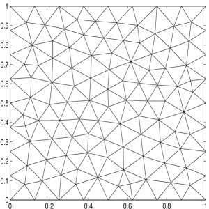
In the first example, we solve the eigenvalue problem (2.2) on the unit square $\Omega=(0,1)\times(0,1)$. In order to investigate the efficiency of the a posteriori error estimate $\eta(\lambda_{i,h},u_{i,h},\mathbf{y}_{h}^{*})$, the guaranteed upper bound $\eta_{h}^{U}(\lambda_{1,h},u_{1,h},\mathbf{y}_{h}^{*})$ of the error estimate $\|u_{1}-u_{1,h}\|_{a}$ and the lower bound $\lambda_{1,h}^{L}$ of the first eigenvalue $\lambda_{1}$, we produce the sequence of finite element spaces on the sequence of meshes which are obtained by the regular refinement (connecting the midpoints of each edge) from an initial mesh. In this example, the initial mesh is showed in Figure 1 which is generated by Delaunay method.

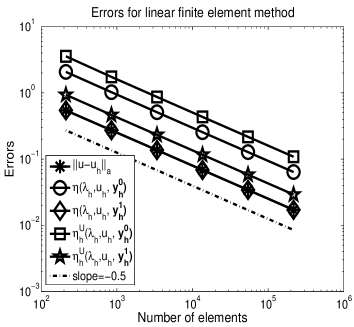
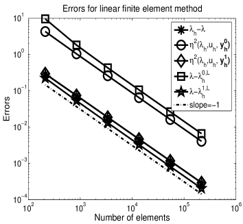
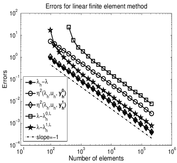
First we solve the eigenvalue problem (2.5) by the linear conforming finite element method and solve the dual problem (5.2) in the finite element space $\mathbf{W}_{h}^{0}$ and $\mathbf{W}_{h}^{1}$, respectively. The corresponding numerical results are presented in Figure 2 which shows that the a posteriori error estimate $\eta(\lambda_{1,h},u_{1,h},\mathbf{y}_{h}^{*})$ is efficient when we solve the dual problem by $\mathbf{W}_{h}^{1}$. Figure 2 also shows the validation of the guaranteed upper bound $\eta_{h}^{U}(\lambda_{1,h},u_{1,h},\mathbf{y}_{h}^{*})$ for the error $\|u_{1}-u_{1,h}\|_{a}$ and the eigenvalue approximation $\lambda_{1,h}^{L}$ is really a guaranteed lower bound for the first eigenvalue $\lambda_{1}=1+2\pi^{2}$ despite the way to solve the dual problem by $\mathbf{W}_{h}^{0}$ or $\mathbf{W}_{h}^{1}$.

Figure 1: The initial mesh for the unit square

Figure 2: The errors for the unit square domain when the eigenvalue problem is solved by the linear finite element method, where $\eta(\lambda_{h},u_{h},\mathbf{y}_{h}^{0})$ and $\eta(\lambda_{h},u_{h},\mathbf{y}_{h}^{1})$ denote the a posteriori error estimates $\eta(\lambda_{1,h},u_{1,h},\mathbf{y}_{h}^{*})$ when the dual problem is solved by $\mathbf{W}_{h}^{0}$ and $\mathbf{W}_{h}^{1}$, respectively, and $\lambda_{h}^{0,L}$ and $\lambda_{h}^{1,L}$ denote the guaranteed lower bounds of the first eigenvalue $\lambda_{1}$ when the dual problem is solved by $\mathbf{W}_{h}^{0}$ and $\mathbf{W}_{h}^{1}$, respectively

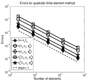
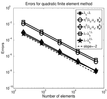
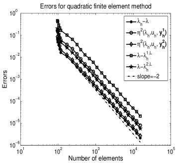
We also solve the eigenvalue problem (2.5) by the quadratic finite element method and solve the dual problem (5.2) with the finite element space $\mathbf{W}_{h}^{1}$ and $\mathbf{W}_{h}^{2}$, respectively. Figure 3 shows the corresponding numerical results. From Figure 3, we can find that the a posteriori error estimate $\eta(\lambda_{1,h},u_{1,h},\mathbf{y}_{h}^{*})$ is efficient when we solve the dual problem by $\mathbf{W}_{h}^{2}$. Figure 3 also shows $\eta_{h}^{U}(\lambda_{1,h},u_{1,h},\mathbf{y}_{h}^{*})$ is really the guaranteed upper bound of the error $\|u_{1}-u_{1,h}\|_{a}$ and the eigenvalue approximation $\lambda_{1,h}^{L}$ is also really a guaranteed lower bound of the first eigenvalue $\lambda_{1}$.

Figure 3: The errors for the unit square domain when the eigenvalue problem is solved by the quadratic finite element method, where $\eta(\lambda_{h},u_{h},\mathbf{y}_{h}^{1})$ and $\eta(\lambda_{h},u_{h},\mathbf{y}_{h}^{2})$ denote the a posteriori error estimates $\eta(\lambda_{1,h},u_{1,h},\mathbf{y}_{h}^{*})$ when the dual problem is solved by $\mathbf{W}_{h}^{1}$ and $\mathbf{W}_{h}^{2}$, respectively, and $\lambda_{h}^{1,L}$ and $\lambda_{h}^{2,L}$ denote the guaranteed lower bounds of the first eigenvalue $\lambda_{1}$ when the dual problem is solved by $\mathbf{W}_{h}^{1}$ and $\mathbf{W}_{h}^{2}$, respectively

In this section, we also check the efficiency of the error estimates $\eta^{2}(\lambda_{i,h},u_{i,h},\mathbf{y}_{h}^{*})$ ($i=2,3$) for the second and third eigenvalues. Tables 1 and 2 show the corresponding numerical results. In Table 1, we solve the eigenvalue problem (2.5) by the linear finite element method and the dual problem (5.2) with the finite element space $\mathbf{W}_{h}^{0}$ and $\mathbf{W}_{h}^{1}$, respectively. In Table 2, the eigenvalue problem (2.5) is solved by the quadratic finite element method and we solve the dual problem (5.2) with the finite element space $\mathbf{W}_{h}^{1}$ and $\mathbf{W}_{h}^{2}$, respectively.

Table 1: The errors for the unit square domain when the eigenvalue problem is solved by the linear finite element method, where $\eta(\lambda_{i,h},u_{i,h},\mathbf{y}_{h}^{0})$ ($i=2,3$) and $\eta(\lambda_{i,h},u_{i,h},\mathbf{y}_{h}^{1})$ denote the a posteriori error estimates $\eta(\lambda_{i,h},u_{i,h},\mathbf{y}_{h}^{*})$ when the dual problem is solved by $\mathbf{W}_{h}^{0}$ and $\mathbf{W}_{h}^{1}$, respectively.

Number of elements	$\lambda_{2,h}-\lambda_{2}$	$\eta^{2}(\lambda_{2,h},u_{2,h},\mathbf{y}_{h}^{0})$	$\eta^{2}(\lambda_{2,h},u_{2,h},\mathbf{y}_{h}^{1})$
208	1.9304e+00	7.2113e+01	1.9875e+00
832	4.8497e-01	1.6651e+01	4.8866e-01
3328	1.2164e-01	4.0794e+00	1.2188e-01
13312	3.0450e-02	1.0147e+00	3.0469e-02
53248	7.6161e-03	2.5337e-01	7.6182e-03
212992	1.9043e-03	6.3322e-02	1.9047e-03
Number of elements	$\lambda_{3,h}-\lambda_{3}$	$\eta^{2}(\lambda_{3,h},u_{3,h},\mathbf{y}_{h}^{0})$	$\eta^{2}(\lambda_{3,h},u_{3,h},\mathbf{y}_{h}^{1})$
208	1.9386e+00	7.0685e+01	1.9968e+00
832	4.8728e-01	1.6198e+01	4.9098e-01
3328	1.2227e-01	3.9655e+00	1.2252e-01
13312	3.0615e-02	9.8627e-01	3.0634e-02
53248	7.6578e-03	2.4625e-01	7.6599e-03
212992	1.9148e-03	6.1543e-02	1.9151e-03

The numerical results in Tables 1 and 2 show that $\eta^{2}(\lambda_{i,h},u_{i,h},\mathbf{y}_{h}^{*})$ ($i=2,3$) is a very efficient error estimator for the eigenvalue approximation $\lambda_{i,h}$ when the error of the dual problem is small compared to the error of the primitive problem. This phenomena is in agreement with Theorem 4.2, Corollary 4.1 and Remark 4.2.

Table 2: The errors for the unit square domain when the eigenvalue problem is solved by the quadratic finite element method, where $\eta(\lambda_{i,h},u_{i,h},\mathbf{y}_{h}^{0})$ ($i=2,3$) and $\eta(\lambda_{i,h},u_{i,h},\mathbf{y}_{h}^{1})$ denote the a posteriori error estimates $\eta(\lambda_{i,h},u_{i,h},\mathbf{y}_{h}^{*})$ when the dual problem is solved by $\mathbf{W}_{h}^{0}$ and $\mathbf{W}_{h}^{1}$, respectively.

Number of elements	$\lambda_{2,h}-\lambda_{2}$	$\eta^{2}(\lambda_{2,h},u_{2,h},\mathbf{y}_{h}^{0})$	$\eta^{2}(\lambda_{2,h},u_{2,h},\mathbf{y}_{h}^{1})$
208	1.3955e-02	4.6633e-01	1.3818e-02
832	9.0239e-04	2.9777e-02	9.0013e-04
3328	5.7163e-05	1.8719e-03	5.7128e-05
13312	3.5934e-06	1.1718e-04	3.5928e-06
53248	2.2519e-07	7.3268e-06	2.2519e-07
Number of elements	$\lambda_{3,h}-\lambda_{3}$	$\eta^{2}(\lambda_{3,h},u_{3,h},\mathbf{y}_{h}^{0})$	$\eta^{2}(\lambda_{3,h},u_{3,h},\mathbf{y}_{h}^{1})$
208	1.4340e-02	4.6548e-01	1.4193e-02
832	9.2527e-04	2.9950e-02	9.2287e-04
3328	5.8616e-05	1.8858e-03	5.8578e-05
13312	3.6855e-06	1.1809e-04	3.6849e-06
53248	2.3101e-07	7.3849e-06	2.3100e-07

5.2 Eigenvalue problem on L-shape domain

In the second example, we solve the eigenvalue problem (2.2) on the L-shape domain $\Omega=(-1,1)\times(-1,1)/[0,1)\times(-1,0]$. Since $\Omega$ has a re-entrant corner, the singularity of the first eigenfunction is expected. The convergence order for the eigenvalue approximation is less than $2$ by the linear finite element method which is the order predicted by the theory for regular eigenfunctions. We investigate the numerical results for the first eigenvalue. Since the exact eigenvalue is not known, we choose an adequately accurate approximation $\lambda_{1}=10.6397238440219$ obtained by the extrapolation method [19] as the exact first eigenvalue for the numerical tests. In order to treat the singularity of the eigenfunction, we solve the eigenvalue problem (2.2) by the adaptive finite element method (cf. [8]). For simplicity, we set $\lambda:=\lambda_{1}$, $u:=u_{1}$, $\lambda_{h}:=\lambda_{1,h}$ and $u_{h}:=u_{1,h}$ in this subsection.

We present this example to validate the results in this paper also hold on the adaptive meshes. In order to use the adaptive finite element method, we define the a posteriori error estimator as follows: Define the element residual $\mathcal{R}_{K}(\lambda_{h},u_{h})$ and the jump residual $\mathcal{J}_{E}(u_{h})$ as follows:

$$\mathcal{R}_{K}(\lambda_{h},u_{h}) := \lambda_{h}u_{h}+\Delta u_{h}-u_{h}\ \ \text{in}\ K\in\mathcal{T}_{h},$$ (5.3)

$$\mathcal{J}_{E}(u_{h}) := -\nabla u_{h}^{+}\cdot\nu^{+}-\nabla u_{h}^{-}\cdot\nu^{-}:=[[\nabla u_{h}]]_{E}\cdot\nu_{E}\ \ \ \text{on}\ E\in\mathcal{E}_{h},$$ (5.4)

where $E$ is the common side of elements $K^{+}$ and $K^{-}$ with outward normals $\nu^{+}$ and $\nu^{-}$, $\nu_{E}=\nu^{-}$.

For each element $K\in\mathcal{T}_{h}$, we define the local error indicator $\eta_{h}(\lambda_{h},u_{h},K)$ by

$$\eta_{h}^{2}(\lambda_{h},u_{h},K):=h_{T}^{2}\|\mathcal{R}_{K}(\lambda_{h},u_{h})\|_{0,K}^{2}+\sum\limits_{E\in\mathcal{E}_{h},E\subset\partial K}h_{E}\|\mathcal{J}_{E}(u_{h})\|^{2}_{0,E}.$$ (5.5)

Then we define the global a posteriori error estimator $\eta_{\rm ad}(\lambda_{h},u_{h})$ by

$$\eta_{\rm ad}(\lambda_{h},u_{h}):=\left(\sum_{K\in\mathcal{T}_{h}}\eta_{h}^{2}(\lambda_{h},u_{h},K)\right)^{1/2}.$$ (5.6)

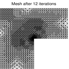
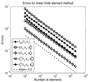
We solve the eigenvalue problem (2.5) by the linear conforming finite element method and solve the dual problem (5.2) in the finite element space $\mathbf{W}_{h}^{0}$ and $\mathbf{W}_{h}^{1}$, respectively. Figure 4 (left) shows the corresponding adaptive mesh. The corresponding numerical results are presented in Figure 5 which shows that the a posteriori error estimate $\eta(\lambda_{h},u_{h},\mathbf{y}_{h}^{*})$ is also efficient even on the adaptive meshes when we solve the dual problem by $\mathbf{W}_{h}^{1}$. Figure 5 also shows the validation of the guaranteed upper bound $\eta_{h}^{U}(\lambda_{h},u_{h},\mathbf{y}_{h}^{*})$ for the error $\|u-u_{h}\|_{a}$ and the eigenvalue approximation $\lambda_{h}^{L}$ is really a guaranteed lower bound of the first eigenvalue despite the way to solve the dual problem by $\mathbf{W}_{h}^{0}$ or $\mathbf{W}_{h}^{1}$.

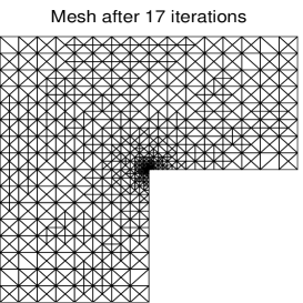
Figure 4: The triangulations after adaptive iterations for L-shape domain by the linear element (left) and the quadratic element (right)

Figure 5: The errors for the L-shape domain when the eigenvalue problem is solved by the linear finite element method, where $\eta(\lambda_{h},u_{h},\mathbf{y}_{h}^{0})$ and $\eta(\lambda_{h},u_{h},\mathbf{y}_{h}^{1})$ denote the a posteriori error estimates $\eta(\lambda_{h},u_{h},\mathbf{y}_{h}^{*})$ when the dual problem is solved by $\mathbf{W}_{h}^{0}$ and $\mathbf{W}_{h}^{1}$, respectively, and $\lambda_{h}^{0,L}$ and $\lambda_{h}^{1,L}$ denote the guaranteed lower bounds of the first eigenvalue when the dual problem is solved by $\mathbf{W}_{h}^{0}$ and $\mathbf{W}_{h}^{1}$, respectively

In this example, we also solve the eigenvalue problem (2.5) by the quadratic finite element method and the dual problem (5.2) with the finite element space $\mathbf{W}_{h}^{1}$ and $\mathbf{W}_{h}^{2}$, respectively. The corresponding adaptive mesh is presented in Figure 4 (right). Figure 6 shows the corresponding numerical results. From Figure 6, we can find that the a posteriori error estimate $\eta(\lambda_{h},u_{h},\mathbf{y}_{h}^{*})$ is efficient when we solve the dual problem by $\mathbf{W}_{h}^{2}$. Figure 6 also shows $\eta_{h}^{U}(\lambda_{h},u_{h},\mathbf{y}_{h}^{*})$ is really the guaranteed upper bound of the error $\|u-u_{h}\|_{a}$ and the eigenvalue approximation $\lambda_{h}^{L}$ is also really a guaranteed lower bound of the first eigenvalue.

Figure 6: The errors for the L shape domain when the eigenvalue problem is solved by the quadratic finite element method, where $\eta(\lambda_{h},u_{h},\mathbf{y}_{h}^{1})$ and $\eta(\lambda_{h},u_{h},\mathbf{y}_{h}^{2})$ denote the a posteriori error estimates $\eta(\lambda_{h},u_{h},\mathbf{y}_{h}^{*})$ when the dual problem is solved by $\mathbf{W}_{h}^{1}$ and $\mathbf{W}_{h}^{2}$, respectively, and $\lambda_{h}^{1,L}$ and $\lambda_{h}^{2,L}$ denote the guaranteed lower bounds of the first eigenvalue when the dual problem is solved by $\mathbf{W}_{h}^{1}$ and $\mathbf{W}_{h}^{2}$, respectively

6 Concluding remarks

In this paper, we give a computable error estimate for the eigenpair approximation by the general conforming finite element methods on general meshes. Furthermore, the guaranteed upper bound of the error estimate for the first eigenfunction approximation and the lower bound of the first eigenvalue can be obtained by the computable error estimate and a lower bound of the second eigenvalue. If the eigenpair approximations are obtained by solving the discrete eigenvalue problem, the computable error estimates are asymptotically exact and we can also give asymptotically lower bounds for the general eigenvalues. Some numerical examples are provided to demonstrate the validation of the guaranteed upper and lower bounds for the general conforming finite element methods on the general meshes (quasi-uniform and regular types [8, 13]). The method here can be extended to other eigenvalue problems such as Steklov, Stokes and other similar types [20, 28]. Especially, we would like to say that the computable error estimate can be extended to the nonlinear eigenvalue problems which are produced from the complicated linear eigenvalue problems. Furthermore, the method in this paper can be used to check the modeling and discretization errors for the models (nonlinear eigenvalue problems) in the density functional theory comes from the linear Schrödinger equation [16, 25]. These will be our future work.

References

• [1] R. Adams, Sobolev Spaces, Academic Press, New York, 1975.
• [2] M. Ainsworth and J. Oden, A posteriori error estimation in finite element analysis, Pure and Applied Mathematics (New York), Wiley-Interscience [John Wiley & Sons, New York, 2000.
• [3] M. G. Armentano and R. G. Durán, Asymptotic lower bounds for eigenvalues by nonconforming finite element method, Electron. Trans. Numer. Anal., 17 (2004), 93-101.
• [4] I. Babuška and J. Osborn, Finite element-Galerkin approximation of the eigenvalues and eigenvectors of selfadjoint problems, Math. Comp. 52 (1989), 275-297.
• [5] I. Babuška and J. Osborn, Eigenvalue Problems, In Handbook of Numerical Analysis, Vol. II, (Eds. P. Lions and P. Ciarlet), Finite Element Methods (Part 1), North-Holland, Amsterdam, 641-787, 1991.
• [6] I. Babuška and W. Rheinboldt, Error estimates for adaptive finite ele- ment computations, SIAM J. Numer. Anal., 15 (1978), 736-754.
• [7] I. Babuška and W. Rheinboldt, A-posteriori error estimates for the finite element method, Int. J. Numer. Methods Eng., 12 (1978), 1597-1615.
• [8] S. Brenner and L. Scott, The Mathematical Theory of Finite Element Methods, New York: Springer-Verlag, 1994.
• [9] F. Brezzi and M. Fortin, Mixed and Hybrid Finite Element Methods, New York: Springer-Verlag, 1991.
• [10] C. Carstensen and D. Gallistl, Guaranteed lower eigenvalue bounds for the biharmonic equation, Numer. Math., 126 (2014), 33-51.
• [11] C. Carstensen and J. Gedicke, Guaranteed lower bounds for eigenvalues, Math. Comp., 83(290) (2014), 2605-2629.
• [12] F. Chatelin, Spectral Approximation of Linear Operators, Academic Press Inc, New York, 1983.
• [13] P. Ciarlet, The Finite Element Method for Elliptic Problem, North-holland Amsterdam, 1978.
• [14] J. Haslinger and I. Hlaváček, Convergence of a finite element method based on the dual variational formulation, Apl. Mat., 21 (1976), 43-65.
• [15] J. Hu, Y. Huang and Q. Lin, The lower bounds for eigenvalues of elliptic operators by nonconforming finite element methods, J. Sci. Comput., 61(1) (2014), 196-221.
• [16] W. Kohn and L. Sham, Self-consistent equations including exchange and correlation effects, Phys. Rev. A, 140 (1965), 4743-4754.
• [17] Q. Lin, F. Luo and H. Xie, A posterior error estimator and lower bound of a nonconforming finite element method, J. Comput. App. Math., 265 (2014), 243-254.
• [18] Q. Lin and H. Xie, The asymptotic lower bounds of eigenvalue problems by nonconforming finite element methods, Math. in Practice and Theory (in Chinese), 42(11) (2012), 219-226.
• [19] Q. Lin and J. Lin, Finite Element Methods: Accuracy and Inprovement, Science Press, Beijing, 2006.
• [20] Q. Lin and H. Xie, Recent results on lower bounds of eigenvalue problems by nonconforming finite element methods, Inverse Problems and Imaging, 7(3), 2013, 795-811.
• [21] Q. Lin, H. Xie, F. Luo, Y. Li, and Y. Yang, Stokes eigenvalue approximation from below with nonconforming mixed finite element methods, Math. in Practice and Theory (in Chinese), 19 (2010), 157-168.
• [22] X. Liu, A framework of verified eigenvalue bounds for self-adjoint differential operators, Appl. Math. Comput., 267 (2015), 341-355.
• [23] X. Liu and S. Oishi, Verifed eigenvalue evaluation for the Laplacian over polygonal domains of arbitrary shape, SIAM J. Numer. Anal., 51(3) (2013), 1634-1654.
• [24] F. Luo, Q. Lin and H. Xie, Computing the lower and upper bounds of Laplace eigenvalue problem: by combining conforming and nonconforming finite element methods, Sci. China Math., 55(5) (2012), 1069-1082.
• [25] R. Martin, Electronic Structure: Basic Theory and Practical Methods, Cambridge University Press, London, 2004.
• [26] P. Neittaanmäki and S. Repin, Reliable methods for computer simulation, Error control and a posteriori estimates, vol. 33 of Studies in Mathematics and its Applications, Elsevier Science B. V., Amsterdam, 2004.
• [27] S. Repin, A posteriori estimates for partial differential equations, vol. 4 of Radon Series on Computational and Applied Mathematics, Walter de Gruyter GmbH & Co. KG, Berlin, 2008.
• [28] I. Šebestová and T. Vejchodský, Two-sided bounds for eigenvalues of differential operators with applications to Friedrichs’, Poincaré, trace, and similar constants, SIAM J. Numer. Anal., 52(1) (2014), 308-329.
• [29] T. Vejchodský, Complementarity based a posteriori error estimates and their properties, Math. Comput. Simulation, 82 (2012), 2033-2046.
• [30] T. Vejchodský, Computing upper bounds on Friedrichs’ constant, in Applications of Mathematics 2012, J. Brandts, J. Chleboun, S. Korotov, K. Segeth, J. Šístek, and T. Vejchodský, eds., Institute of Mathematics, ASCR, Prague, 2012, pp. 278-289.
• [31] R. Verfürth, A review of a posteriori error estimation and adaptive mesh-refinement techniques, Wiley-Teubner, Chichester/Stuttgart, 1996.
• [32] H. Xie, A multigrid method for eigenvalue problem, J. Comput. Phys., 274 (2014), 550-561.
• [33] H. Xie, A type of multilevel method for the Steklov eigenvalue problem, IMA J. Numer. Anal., 34 (2014), 592-608.
• [34] Y. Yang, Z. Zhang and F. Lin, Eigenvalue approximation from below using non-forming finite elements, Sci. China. Math., 53 (2010), 137-150.
• [35] Z. Zhang, Y. Yang and Z. Chen, Eigenvalue approximation from below by Wilson’s element, Chinese J. Numer. Math. Appl., 29 (2007), 81-84.