Collective behavior of quorum-sensing run-and-tumble particles in confinement

Abstract

We study a generic model for quorum-sensing bacteria in circular confinement. Every bacterium produces signaling molecules, the local concentration of which triggers a response when a certain threshold is reached. If this response lowers the motility then an aggregation of bacteria occurs, which differs fundamentally from standard motility-induced phase separation due to the long-ranged nature of the concentration of signal molecules. We analyze this phenomenon analytically and by numerical simulations employing two different protocols leading to stationary cluster and ring morphologies, respectively.

Introduction. Motility and locomotion are basic as well as challenging tasks for microorganisms exploring complex aqueous environments Lauga and Powers (2009), and nature has developed a range of diverse strategies for this purpose. For example, the sperm cells of sea urchins find the egg by moving along helical paths, the curvature of which is controlled by the concentration of a chemoattractant Friedrich and Jülicher (2007); Jikeli et al. (2015). On the other hand, bacteria might use quorum sensing to respond to changes in their environment Miller and Bassler (2001). The probably most famous example is the marine bacterium V. fischeri, which controls bioluminescence in accordance with its population density. To this end bacteria measure the local concentration of certain signal molecules, called autoinducers, which are emitted by other bacteria.

Moving along a chemical gradient of chemoattractants or repellents is called chemotaxis. The arguably most famous and best studied model for chemotaxis is the Keller-Segel model Keller and Segel (1970); Brenner et al. (1998), which consists of two coupled partial differential equations, one for the density of diffusing bacteria and one for the concentration of signal molecules. The Keller-Segel model has become a cornerstone to study pattern formation (such as rings and spots in E. coli Adler (1966); Budrene and Berg (1991) and S. typhimurium Woodward et al. (1995)) and self-organization in general Hillen and Painter (2009). It is not restricted to bacteria, e.g., chemotactic behavior has also been reported for self-propelled colloidal particles Paxton et al. (2004); Theurkauff et al. (2012); Pohl and Stark (2014), which are phoretically driven by the catalytic decomposition of, e.g., hydrogen peroxide playing the role of the chemical signal.

It has been argued that chemotaxis is not the only route to self-organization of motile cells and bacteria, and that similar patterns are observed in an arrested motility-induced phase transition in combination with bacteria reproduction Cates et al. (2010); Cates (2012). Such a scenario relies on a positive feedback through a density-dependent motility with “slow” bacteria in dense environments Cates and Tailleur (2015) so that they may move against a density gradient. It allows an effective equilibrium description in terms of a coarse-grained population density as long as the motility is a local function, which seems to be a good assumption for short-ranged physical interactions, e.g., for self-propelled colloidal particles Buttinoni et al. (2013); Speck et al. (2014, 2015). However, for quorum-sensing bacteria the motility is no longer a function of the density but of the local concentration of the autoinducers. The dependence of the local concentration on the sources (or sinks in the case of catalytic swimmers) is strongly non-local and long-ranged, which precludes a mapping onto equilibrium phase separation.

In this Letter we study how patterns can emerge based on motility changes even in populations with a conserved number of members. To this end, we combine a simple model for bacteria dynamics with quorum sensing. Bacteria (or more generally, particles) solely interact via signaling molecules. Particles are confined and we observe aggregation in the center of the confinement mediated by the autoinducers (see Refs. 20; 21 for experiments and numerical results in more complex confining geometries). This aggregation is in contrast to other collective behavior of confined active particles like the self-organized pump in a harmonic trap Nash et al. (2010); Hennes et al. (2014) and the aggregation at walls Fily et al. (2014); Yang et al. (2014); Smallenburg and Löwen (2015). By combining numerical simulations and analytical theory, we show that the aggregation is determined by a set of universal parameters that depend on system size.

Model. We model the bacteria as run-and-tumble particles moving in two dimensions above a substrate. The dynamics mimics straight “runs” due to, e.g., synchronized flagella interrupted by random “tumble” events Polin et al. (2009); Reigh et al. (2012). The equations of motion are

$$\dot{\mathbf{r}}_{k}=v\mathbf{e}_{k}+\mu_{0}\mathbf{F}_{k},$$ (1)

where $\mathbf{F}_{k}$ is the force and $\mu_{0}$ the bare mobility. Every particle has an orientation $\mathbf{e}_{k}=(\cos\varphi_{k},\sin\varphi_{k})^{T}$ along which it is propelled with speed $v$. This orientation remains fixed for an exponentially distributed random waiting time with mean $\tau_{\text{r}}$, after which a tumble event occurs. We assume the tumbling to occur instantaneously and pick a new, uniformly distributed, orientation $\varphi_{k}$ Schnitzer (1993).

Every particle produces autoinducers with rate $\gamma$. These signal molecules with concentration $\hat{c}(\mathbf{r},t)$ diffuse with diffusion coefficient $D_{\text{c}}$. While the actual particles move in two dimensions and are confined by a circular confinement with radius $R$ (e.g., due to a semi-permeable membrane), the autoinducers can penetrate this wall and permeate the semispace above the substrate. The time evolution of the concentration is thus described by

$$\partial_{t}\hat{c}=D_{\text{c}}\nabla^{2}\hat{c}+\gamma\sum_{k=1}^{N}\delta(\mathbf{r}-\mathbf{r}_{k}).$$ (2)

In the following we assume that the molecular diffusion is much faster than the motion of the much larger particles so that there is an instantaneous stationary concentration of autoinducers

$$\hat{c}(\mathbf{r})=\frac{\gamma}{4\pi D_{\text{c}}}\sum_{k=1}^{N}\frac{1}{|\mathbf{r}-\mathbf{r}_{k}|}.$$ (3)

Due to the autoinducers eventually leaving the confinement the concentration remains finite. The collective behavior of the particles is controlled through $\tau_{\text{r}}(\mathbf{r})=\tau_{\text{r}}(\hat{c}(\mathbf{r}))$ and $v(\mathbf{r})=v(\hat{c}(\mathbf{r}))$, which both can vary spatially through their dependence on the concentration of autoinducers $c(\mathbf{r})$. Averaging over particle positions gives the average concentration $c(\mathbf{r})=\langle\hat{c}(\mathbf{r})\rangle$.

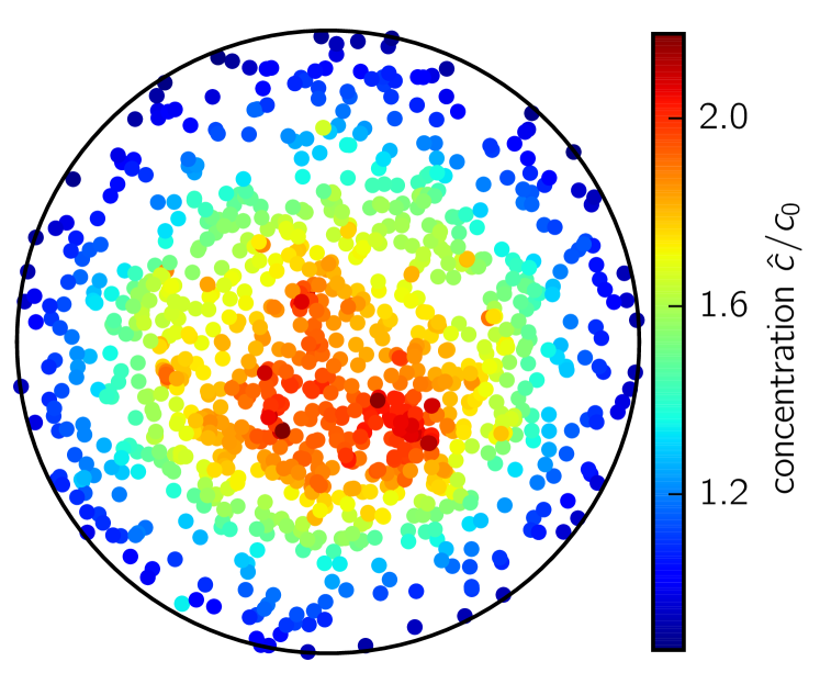
Figure 1: Snapshot of a configuration with $N=1000$ quorum-sensing run-and-tumble particles. The color code indicates the local concentration $\hat{c}$ of signal molecules felt by each particle.

For the numerical integration of Eq. (1) we employ a fixed time step $\delta t$. After propagating all particles along their orientation, a new random orientation is assigned with probability $\delta t/\tau_{\text{r}}$. Instead of an ideal hard wall, we employ the Weeks-Chandler-Andersen (WCA) potential Weeks et al. (1971) leading to a small but finite “thickness” $d=5\cdot 10^{-3}R$ of the wall. Particles with outward-pointing orientations remain trapped within the wall until the orientations, due to their rotational diffusion, point inwards again. Fig. 1 shows a snapshot of the system for $N=1000$ particles after relaxation to the steady state [SM].

Mean-field theory. We first consider run-and-tumble particles that only interact via sensing the autoinducers. It is then sufficient to consider the one-point density $\psi(\mathbf{r},\varphi,t)$ of position and orientation, which obeys the dynamical equation

$$\partial_{t}\psi=-\nabla\cdot(v\mathbf{e}\psi)-\frac{1}{\tau_{\text{r}}}\psi+\frac{1}{2\pi\tau_{\text{r}}}\rho$$ (4)

with particle density $\rho(\mathbf{r},t)=\int_{0}^{2\pi}\mathrm{d}\varphi\;\psi(\mathbf{r},\varphi,t)$ corresponding to the zeroth moment of $\psi$. The first moment $\mathbf{p}(\mathbf{r},t)=\int_{0}^{2\pi}\mathrm{d}\varphi\;\mathbf{e}\psi(\mathbf{r},\varphi,t)$ describes the orientational density of the run-and-tumble particles. From Eq. (4) we obtain the adiabatic solution $\mathbf{p}=-\frac{1}{2}\tau_{\text{r}}\nabla(v\rho)$ dropping the time derivative and neglecting the dependence on the second moment.

For the analytical treatment we further approximate $v=v(c)$ and $\tau_{\text{r}}=\tau_{\text{r}}(c)$, i.e., the response depends on the local average concentration $c(\mathbf{r})$. It is instructive to first consider the Keller-Segel model, which, assuming constant $\tau_{\text{r}}$, follows in the limit of a weak perturbation of the velocity $v(c)\approx\bar{v}+v^{\prime}(\bar{c})(c-\bar{c})$ around a uniform concentration $\bar{c}$. Eq. (4) implies $\partial_{t}\rho=-\nabla\cdot(v\mathbf{p})$, which leads to

$$\partial_{t}\rho=\nabla\cdot(D\nabla\rho-\chi\rho\nabla c)$$ (5)

after inserting the adiabatic solution for the orientational density. This is the Keller-Segel model together with $\partial_{t}c=D_{\text{c}}\nabla^{2}c+\gamma\rho\delta(z)$, where the source term in Eq. (2) has been replaced by the density $\rho_{\text{3D}}(\mathbf{r},z)=\rho(\mathbf{r})\delta(z)$. The two coefficients $D=\frac{1}{2}\tau_{\text{r}}\bar{v}^{2}$ and $\chi=-\frac{1}{2}\tau_{\text{r}}\bar{v}v^{\prime}(\bar{c})$ are the effective diffusivity and chemotactic sensitivity, respectively. This result demonstrates that chemotactic behavior can be achieved simply by changing the magnitude of the speed depending on the difference between the local and a fixed reference concentration without sensing the concentration gradient.

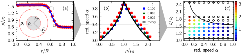
Figure 2: Clustering of slow particles. (a) The particle density $\rho(r)$ for reduced speed $\alpha=0.4$ and persistence length $\ell=0.01$ obtained numerically for $N=1000$ particles (symbols) and from the mean-field theory (dashed line). The solid line is a fit to Eq. (11). A sketch of a cluster with radius $r_{\ast}$ and density $\rho_{1}$ is shown in the inset, where $\rho_{2}$ is the density of the dilute region surrounding the cluster. (b) Densities $\rho_{1}$ (dense, right branch) and $\rho_{2}$ (dilute, left branch) for threshold $\bar{c}=1.45c_{0}$. The numerical results slightly depend on the persistence length $\ell$, still the overall agreement with the theoretical prediction is excellent. (c) Numerical phase diagram of reduced speed $\alpha$ vs. threshold $\bar{c}$ for $\ell=0.01$. The color bar indicates the density difference $(\rho_{1}-\rho_{2})/\rho_{0}$, whereas open circles indicate that no formation of a cluster has occurred. Also shown is the theoretical prediction (solid lines).

In the following, however, we are rather interested in collective effects that arise because of large (discontinuous) changes of the speed due to some particles reaching a threshold, which is thus beyond the scope of the Keller-Segel model. In the steady state, $\partial_{t}\psi=0$ and we obtain from Eq. (4)

$$\mathbf{p}=-\frac{\tau_{\text{r}}}{2}\nabla(v\rho),\qquad 0=\nabla\cdot(v\mathbf{p}),$$ (6)

where we have neglected the dependence on the second moment. For simplicity, the confinement is now modeled through the no-flux boundary condition $\mathbf{n}\cdot\mathbf{p}|_{R}=0$ with wall normal $\mathbf{n}$, which ignores the trapping of particles at the wall due to their persistent motion. To compare the theory with the numerical results, we define the effective bulk density $\rho_{0}=N_{\text{bulk}}/(\pi R^{2})$ with $N_{\text{bulk}}$ the average number of run-and-tumble particles inside $r<R$ determined in the simulations.

Exploiting the mentioned time-scale separation between molecular diffusion and particle motion, the concentration of autoinducers follows from Eq. (2) with $\partial_{t}c=0$ and the source term again replaced by the density $\rho_{\text{3D}}(\mathbf{r},z)=\rho(\mathbf{r})\delta(z)$, $\nabla^{2}c(\mathbf{r})=-(\gamma/D_{\text{c}})\rho(\mathbf{r})\delta(z)$, which is Poisson’s equation. Since the concentration $c(\mathbf{r})$ determines the speed via $v(c)$ it is coupled with Eq. (6), which can now be solved for the density profile $\rho(r)$. In the remainder of this Letter we will discuss the two situations of one and two thresholds.

Piecewise constant speed. We now specialize to a piecewise constant speed $v(c)$. Suppose that there are two regions with different speeds. Within each region we find $\nabla\cdot\mathbf{p}=0$ from Eq. (6) and hence the normal components of $\mathbf{p}$ across the interface have to be equal. For non-vanishing $\mathbf{p}$ this would imply a steady particle current, which is excluded by the no-flux boundary condition. Hence, we conclude that $\mathbf{p}=0$ and, within our theory neglecting fluctuations, $v\rho=\text{const}$. Interestingly, the reorientation time $\tau_{\text{r}}$ drops out and does not influence the steady state. This is quite in contrast to self-propelled particles with volume exclusion, the collective behavior of which is strongly influenced by orientation relaxation Cates and Tailleur (2015); Speck et al. (2015).

Specifically, we introduce a threshold concentration $\bar{c}$ above which the particles slow down by a factor $\alpha\leqslant 1$,

$$v(\hat{c})=\begin{cases}v_{0}&(\hat{c}<\bar{c}),\\ v_{0}\alpha&(\hat{c}\geqslant\bar{c})\end{cases}$$ (7)

with reference speed $v_{0}$. In the following, the importance of the directed motion is captured by the persistence length $\ell=v_{0}\tau_{\text{r}}/R$ divided by the radius of the confinement. Due to the slow decay of $\hat{c}(\mathbf{r})$, we expect that the steady state will have a radial symmetry with an inner dense cluster and a dilute outer region. In Fig. 2(a) the density profiles predicted by the theory and measured in the simulations are shown for $\alpha=0.4$ and $N=1000$ particles. It clearly shows a higher inner density corresponding to the cluster and a lower outer density.

The theoretical density is a step function that can be obtained as follows. The radius $r_{\ast}$ of the cluster is determined by the condition $c(r_{\ast})=\bar{c}$. Since $v\rho=\text{const}$, the density in both regions is constant with dilute density $\rho_{2}=\alpha\rho_{1}$. Taking into account the conservation of the bulk density

$$\rho_{0}=\frac{1}{\pi R^{2}}\int_{0}^{R}\mathrm{d}r\;2\pi r\rho(r),$$ (8)

the density of the cluster follows as

$$\rho_{1}=\frac{\rho_{0}}{\alpha+(1-\alpha)x_{\ast}^{2}}$$ (9)

with $x_{\ast}=r_{\ast}/R$. The radially symmetric solution of the Poisson equation reads

$$c(r)=\frac{\gamma}{\pi D_{\text{c}}}\int_{0}^{R}\mathrm{d}r^{\prime}\;\mathcal{K}(r^{\prime}/r)\rho(r^{\prime})$$ (10)

with kernel $\mathcal{K}(x)=xK(x^{2})$ for $x<1$ and $\mathcal{K}(x)=K(x^{-2})$ for $x>1$, where $K(x)$ is the complete elliptic integral of the first kind. Inserting the step profile $\rho(r)$ we determine self-consistently the radius $r_{\ast}$ of the cluster and thus $\rho_{1}$ and $\rho_{2}$ for given $\bar{c}$, $\alpha$, and $\rho_{0}$. There is a lower bound $c_{0}<\bar{c}$ to the threshold below which no clustering is possible. It is obtained by considering a homogenous density $\rho_{1}=\rho_{0}$ with interface at $r_{\ast}=R$ and thus $c_{0}=c(R)=\gamma\rho_{0}R/(\pi D_{\text{c}})$.

In contrast to the theoretical step profiles, the numerical profiles show a finite interfacial width due to fluctuations. Despite the fact that these fluctuations are not accounted for in the theory, the densities of the cluster and the dilute outer region are predicted quite accurately (at least for not too small persistence lengths). The full profile is well fitted by the empirical expression

$$\rho(r)=\frac{\rho_{1}+\rho_{2}}{2}-\frac{\rho_{1}-\rho_{2}}{2}\tanh\left(\frac{r-r_{\ast}^{\prime}}{2w}\right),$$ (11)

from which the densities $\rho_{1,2}$ and the width $w$ of the profile can be extracted. Fitted positions $r_{\ast}^{\prime}<r_{\ast}$ of the interface are smaller than the prediction $r_{\ast}$. In Fig. 2(b) the densities $\rho_{1,2}$ are plotted as a function of reduced speed $\alpha$ for fixed threshold concentration $\bar{c}=1.45c_{0}$ and several values of the persistence length, which show good agreement with the theoretical curve.

The phase diagram in the $\alpha$–$\bar{c}$ plane is shown in Fig. 2(c). Besides the lower threshold $c_{0}$ there is also an upper threshold depending on $\alpha$ beyond which no clustering is possible anymore. After a bit of algebra one finds for the concentration at the interface

$$\frac{c_{\ast}}{c_{0}}=\frac{\alpha E(x_{\ast}^{2})+(1-\alpha)x_{\ast}}{\alpha+(1-\alpha)x_{\ast}^{2}}$$ (12)

with $E(x)$ the complete elliptic integral of the second kind. This function has a maximum for $0\leqslant x_{\ast}\leqslant 1$, which means that a threshold higher than this maximum cannot be reached and, therefore, no clustering is possible. Again, the theoretical predictions for the parameter space where clustering is possible agree very well with the numerical observations as shown in Fig. 2(c).

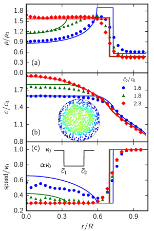
Figure 3: Formation of a ring for two thresholds $\bar{c}_{2}>\bar{c}_{1}$. Shown is (a) the particle densities $\rho(r)$, (b) the concentration profiles $c(r)$, and (c) the actual average speeds $\langle v(\hat{c})\rangle$ as functions of the radial distance $r/R$ for three different values of the upper threshold $\bar{c}_{2}$ with the lower threshold $\bar{c}_{1}=1.4c_{0}$ held fixed. Symbols indicate simulation results for $N=1000$ particles, solid lines correspond to the mean-field predictions. Parameters are: persistence length $\ell=0.01$ and reduced speed $\alpha=0.3$. The inset in (b) shows a snapshot of the ring ($\bar{c}_{2}=1.6c_{0}$, colors as in Fig. 1), in the inset of (c) the protocol is sketched.

Rings. More complicated morphologies can also be realized. To this end we study numerically the effect a second threshold $\bar{c}_{2}>\bar{c}_{1}$ has on the clustering, where for concentrations $\hat{c}\geqslant\bar{c}_{2}$ the particles again move with the higher speed $v_{0}$. The resulting profiles for density $\rho(r)$, concentration $c(r)$, and actual speed $\langle v(\hat{c})\rangle$ are shown in Fig. 3 for a fixed first threshold $\bar{c}_{1}=1.4c_{0}$. If $\bar{c}_{2}$ lies outside the region indicated in Fig. 2(c) where clustering is possible then basically no change is observed. If the second threshold lies within the clustering region the inner part of the cluster is depleted, leading to the formation of a stationary dense ring [SM]. Such rings have been observed, e.g., for E. coli Adler (1966) but have been attributed to metabolizing the chemoattractant.

Fig. 3(b) shows the corresponding average concentrations $c(r)$ of the autoinducers. While these are roughly independent of $\bar{c}_{2}$ outside the ring, the concentrations saturate at the second threshold $\bar{c}_{2}$ inside the ring. Particles that locally cross the threshold move faster so that there is an effective “pressure” to reduce the inner density. Indeed, Fig. 3(c) shows that the measured average speed $\langle v(\hat{c})\rangle$ is higher than $\alpha v_{0}$ in the inner region, dropping with increasing $r$. The density maximum coincides with the minimum of the speed before the speed again increases going towards the dilute region. While we do not have closed analytical expressions, we can still solve the mean-field equations numerically, whereby the speed varies between $v_{0}\alpha$ and $v_{0}$ and the density follows such that the product $v\rho$ remains constant. As shown in Fig. 3, the mean-field solution correctly captures the qualitative behavior with an inner region where $v>v_{0}\alpha$, a ring (of finite width) within which $v=v_{0}\alpha$, and a sharp interface to the dilute outer region.

Conclusions. To conclude, we have presented a quantitative theory for the collective behavior of quorum-sensing run-and-tumble particles. For one threshold we have derived specific expressions for the cluster morphology in circular confinement and we have confirmed these theoretical predictions in numerical simulations. For a second threshold we have found the formation of a ring, which is also correctly described by the mean-field theory. Patterns typically ascribed to chemotaxis Budrene and Berg (1991); Woodward et al. (1995) or motility-induced phase separation Cates et al. (2010) could thus also be the result of a quorum-sensing mechanism that changes the motility of single microorganisms in response to environmental changes. In contrast to (effective) equilibrium phase separation, the densities $\rho_{1,2}\propto\rho_{0}$ are proportional to the global density. Moreover, the lower threshold $c_{0}\propto R$ depends on the system size $R$ due to the long-ranged concentration profile of the signaling molecules, which implies that clustering in a sufficiently large system is suppressed. As a first step we have considered the most basic combination of quorum sensing with a simplified model of directed motion. It will be interesting to explore other morphologies and to study the basic mechanism for aggregation in more realistic models and test the validity of the scenario we have found.