On the dispute between Boltzmann and Gibbs entropy
Abstract
The validity of the concept of negative temperature has been recently challenged by arguing that the Boltzmann entropy (that allows negative temperatures) is inconsistent from a mathematical and statistical point of view, whereas the Gibbs entropy (that does not admit negative temperatures) provides the correct definition for the microcanonical entropy. Here we prove that the Boltzmann entropy is thermodynamically and mathematically consistent. Analytical results on two systems supporting negative temperatures illustrate the scenario we propose. In addition we numerically study a lattice system to show that negative temperature equilibrium states are accessible and obey standard statistical mechanics prediction.
- PACS numbers
-
05.20.-y, 05.20.Gg, 05.30.-d, 05.30.Ch
keywords:
Statistical Mechanics, Microcanonical Ensemble1 Introduction
The concept of negative absolute temperature was111This was not the first place where negative temperatures have been considered, in fact [1] two years before proposed the existence of negative temperatures in order to explain the formation of large scale vortices by clustering of small ones in hydrodynamic systems. invoked to explain the results of experiments with nuclear-spin systems carried out by Pound [2], Purcell and Pound [3] and Ramsey and Pound [4]. Shortly after these experiments, Ramsey [5] discussed the thermodynamic implications of negative absolute temperature and their meaning in statistical mechanics, thereby granting this concept a well-grounded place in physics [6, 7].
The microcanonical ensemble, which provides the statistical description of an isolated system at equilibrium, is the most appropriate venue to discuss negative temperatures. In this ensemble, the thermodynamic quantities, like temperature and specific heat, are derived from the entropy through suitable thermodynamic relations. For instance, the inverse temperature is proportional to the derivative of the entropy with respect to the energy. In equilibrium statistical mechanics, there are at least two commonly accepted definitions of entropy: the Boltzmann entropy is proportional to the logarithm of the number of microstates in a given “energy shell”, whereas the Gibbs entropy is proportional to the logarithm of the number of microstates up to a given energy. The debate as to which of these definitions of entropy is the correct one has been going on for a long time [8, 9, 10, 11, 12, 13, 14, 15, 16, 17], although the general consensus is that they are basically interchangeable. In fact, for standard systems222 With “standard system” we mean a system with unbounded energy from above for which the energy goes to infinity when one of the canonical coordinates goes to infinity. with a large number of degrees of freedom they are practically equivalent [18]. Full equivalence is obtained in the thermodynamic limit.
The existence of negative-temperature states provides a major bone of contention in the debate. In fact, negative temperatures emerge in the Boltzmann description whenever the number of microstates in a given energy shell is a decreasing function of the relevant energy. On the contrary, the Gibbs temperature can never be negative, since the number of microstates having energy below a given value is always a non-decreasing function of such value. Thus, systems admitting negative (Boltzmann) temperatures provide an ideal context to address the matter of the correct definition of entropy.
Recently [19, 20, 21] it was argued that for a broad class of physical systems, including standard classical Hamiltonian systems, only the Gibbs entropy yields a consistent thermodynamics, and that, consequently, negative temperatures are not achievable within a standard thermodynamical framework. In this respect, what is usually referred to Boltzmann temperature would not possess the required properties for a temperature [19, 22, 23, 24, 20, 25, 26]. These and other related arguments [27, 28, 29] have been contended [30, 31, 32, 33, 34], in what has become a lively debate.
In the present manuscript, at first we focus on the class of systems whose canonical
(or, possibly, grand canonical) ensemble is equivalent to the microcanonical ensemble.
Thus we implicitly exclude non-extensive systems, and systems at the first-order phase
transitions.
We show that such equivalence can be rigorously satisfied only if the thermodynamics
of the latter ensemble is derived by the Boltzmann entropy. For such systems we show
that the Boltzmann temperature provides
a consistent description with those of the canonical
and grand canonical ensembles. Therefore we conclude that, also in the case of
isolated systems for which a comparison between different statistical ensembles is not
possible, the Boltzmann entropy provides the correct description.
Later, we focus on a general system and we prove that the Boltzmann entropy is
thermostatistically consistent and does not violate any fundamental condition for
the microcanonical entropy.
The outline of the paper is the following. In Sec. 2 we summarize the essential features of systems in which negative Boltzmann temperatures are expected. In Sec. 3 we consider an isolated Hamiltonian system and, under the hypothesis of ergodicity, we show that only for the Boltzmann entropy all the thermodynamic quantities can be measured as time averages (along the dynamics) of suitable functions. In Sec. 4 we prove that, for systems whose canonical and microcanonical ensembles are equivalent, the thermodynamically consistent definition for the temperature is the one derived with the Boltzmann entropy. Furthermore we show that, in the thermodynamic limit, the Gibbs and Boltzmann temperatures do coincide when the latter is positive whereas the inverse Gibbs temperature is identically null in the region where Boltzmann provides negative values for the temperature. In Sec. 5 we recall the critique of consistency of Boltzmann entropy raised recently in literature and, in Sec. 6 we prove that the Boltzmann entropy is consistent from a mathematical and thermodynamical point of view. In section 7, we give two examples of systems supporting negative Boltzmann temperatures for which the grand-canonical (or canonical) ensemble and the microcanonical description given by the Boltzmann entropy do agree on the whole parameter space and on the complete range of values of the energy-density. We show that the equipartition theorem fails for system with negative Boltzmann temperatures in Sec. 8. In Sec. 9 we show through numerical simulations on a specific system, that negative temperatures are accessible. We show that, irrespective of the sign of the temperature, a large microcanonical lattice acts as a thermostat for a small grand canonical sublattice, and this confirms the ensemble equivalence. Furthermore, we have shown that, irrespective of the sign of the temperature, two isolated systems at equilibrium at different inverse temperatures, reach an equilibrium state at an intermediate inverse temperature, after that they are brought in contact.
2 Negative temperatures
The microcanonical ensemble describes the equilibrium properties of an isolated system, that is to say in which energy, and possibly further quantities, are conserved. Within the microcanonical description, all the thermodynamic quantities are derived from the entropy, for instance the inverse temperature of the system is defined as
| (1) |
where is the Boltzmann constant and is the entropy density corresponding to a given energy density . The two alternative definitions for the entropy used in equilibrium statistical mechanics are ascribed to Boltzmann and Gibbs333We refer to Ref. [35] for historical details.. According to Boltzmann’s definition
| (2) |
where is the density of microstates at a fixed value energy density and, possibly, at a fixed value of the additional conserved quantities, is a constant with the same dimension as , and is the number of degrees of freedom in the system. The Gibbs entropy is
| (3) |
where is the number of microstates with energy density less than or equal to and, possibly, at a fixed value of the additional conserved quantities. It is known that in the thermodynamic limit these two definitions of entropy lead to equivalent thermodynamic results in “standard” systems [36]. So far, these two entropy definitions have been used in an alternative (interchangeable) way in statistical mechanics, by resorting to the most suitable form depending on the specific problem considered. These two entropy definitions are connected by the relation between and
| (4) |
Since , Gibbs’ temperatures are not negative and consequently the two entropies have incompatible outcomes if applied to systems that admit negative Boltzmann temperatures.
A necessary (although not sufficient) condition for a system for having negative temperatures is the boundedness of the energy (as in the case of nuclear-spin systems discussed by Pound et al), in this case a local maximum inside the system’s density energy interval of the Boltzmann entropy is not forbidden and, both positive and negative Boltzmann temperatures are possible.
Hamiltonians with bounded energies can also be characterized by the existence of more than one first integral of motion and, for this reason, in addition to the statistical mechanics of systems with one first integral, we will consider also the case of systems with more then one first integrals. Within the latter class for instance there are models usually employed for describing ultracold atoms. The possibility of observing negative temperature states in ultracold systems, has been theoretically predicted by some authors with different approaches [37, 38, 39] and, the experimental evidence of the existence of states for motional degrees of freedom of a bosonic gas at negative (Boltzmann) temperatures, have been achieved a few years ago by Braun et al. [40]. The interpretation of such experimental results has been contested in [19]. Successively [20, 21] it has been argued that for a broad class of systems –that includes all “standard classical Hamiltonian systems”– only the Gibbs entropy satisfies all three thermodynamic laws exactly. These papers have engendered a glowing debate between supporters of the Gibbs entropy [23, 24, 25, 26, 22, 20, 28, 29, 21, 34] and those considering correct the Boltzmann entropy [31, 32, 30, 41, 42, 43, 44, 45, 34, 46].
3 Dynamics and statistical mechanics for classical systems
Let us consider first a generic classical many-particle system described by an autonomous Hamiltonian , in which the energy is the sole first integral of motion. The Boltzmann entropy density in this case is given by
| (5) |
whereas the one of Gibbs is
| (6) |
where is the Dirac function and is the Heaviside function.
As a consequence of the conservation of energy, the system dynamics takes place on energy-level sets. From Liouville theorem it descends that the measure of the Euclidean volume is preserved by the dynamics and this induces a measure conserved on each energy level set of energy density which is given by [47, 48]
| (7) |
where is the Euclidean measure induced on and is the Euclidean norm.
This means that, under the hypothesis of ergodicity, the averages of each dynamical observable of the system can be equivalently measured along the dynamics as
| (8) |
or as average on the hypersurface according to
| (9) |
Now, it is reasonable to expect that the temperature, the specific heat, and the other thermodynamic observables could be measured as time averages of suitable observables along the dynamics, in a way analogous to Eq. (8). Consequently, when ergodicity holds, the measures of these quantities have to be derived from averages upon the energy level sets , according to Eq. (9). Furthermore, temperature, specific heat and other thermodynamic quantities depend on derivatives of the microcanonical entropy with respect to energy. Therefore, they are computed by means of a functional of the form (9) if and only if the microcanonical entropy is defined à la Boltzmann. This fact is proven by Rugh [49] in the case of many-particle systems for which the Hamiltonian is the only conserved quantity, and in Ref. [50] and Ref. [51] for the case of two and conserved quantities, respectively.
For instance, in the simpler case studied in Ref. [49] e.g., it results
and from the definition (1) in the case of Boltzmann we obtain 444The Federer-Laurence derivation formula [52, 53] is , where .
| (10) |
where 555 Higher derivatives of respect to are computed by means the Federer-Laurence formula [52, 53] that leads to averages similar to the one in Eq. (9).. In the case of the expression for the inverse temperature is
| (11) |
where , that cannot be expressed in the form (9). In other words, by adopting the Gibbs entropy definition when ergodicity holds true, one has to trust in the very singular fact that time averages of thermodynamic quantities taken along the dynamics (and then on the energy level set ) coincide with the averages of quantities taken on a set that includes all the energy levels below to the one on which the dynamics takes place, analogously to Eq. (11) of the inverse temperature666In addition to the case of the inverse temperature, the same scenario hold for the chemical potential..
In the case of , one could suggest that the Gibbs temperature can be measured as a microcanonical average by resorting to the equipartition theorem. Nevertheless, as we will show in Sec. 8, for instance in the case of systems with negative Boltzmann temperatures, the “standard” equipartition theorem fails. This is a first signal of inconsistency for the Gibbs entropy.
It is worth emphasizing that in the case of conserved quantities, a geometric structure similar to the one of Eq. (10) keeps on to be valid. In fact, in Ref. [50] it has been considered the case by studying a general classical autonomous many-body Hamiltonian system, whose coordinates and canonical momenta are indicated with , and for which is a further conserved quantity in involution with . For such a system, the motion takes place on the manifolds , where are subsets of where is constant. In Ref. [50] it is shown that
| (12) |
where is the volume form of , and
| (13) |
Furthermore, in [50] it is derived the generalization of (10) that gives the microcanonical inverse temperature for these systems, it results
| (14) |
where the complicated functional is now
| (15) |
that is given in terms of the unitary vectors and through the vector , from which is defined the unitary vector that appears in Eq. (15). Remarkably, by exchanging and in expression (15) the functional so obtained allows to measure the chemical potential of the system. This fact shows a further “esthetic advantage” of the Boltzmann entropy: it leads to expressions formally identical independently from the number of conserved quantities.
4 Comparison between statistical ensembles
In a statistical description of a many-body system, temperature has a different meaning depending on the statistical ensemble. In the canonical ensemble and in the grand-canonical one, (inverse) temperature is just a Lagrangian parameter that is introduced in order to fix the mean energy. On the contrary, in the microcanonical ensemble the temperature is a quantity derived from the entropy density , according to the relation . Therefore it is clear that will depend on the entropy definition assumed within the microcanonical statistical description. The main point here is that the meaning of temperature cannot be reduced to the issue of the coherent definition inside to microcanonical ensemble, at least if there is equivalence of ensembles. In the latter case, one expects that temperature, or more in general thermodynamics, defined for a system by two microscopic models, for instance canonical and microcanonical, coincide in the thermodynamic limit and they coincide with the experimentally known thermodynamics of such system [54]. This amounts to requiring that the thermodynamics of a large isolated (microcanonical) system and the thermodynamics of a “small” (even if big enough) subsystem of it coincide. In fact, in the thermodynamic limit, the complement of the subsystem, acts on it as a thermostat and the subsystem is well described in the canonical ensemble. The problem of equivalence of ensembles is only incompletely solved [55], for instance it is known that systems with long-range interaction can violate this equivalence. In fact, for this class of systems the energy is not extensive: a system cannot be divided into independent macroscopic parts at variance of the case of the short-range interaction. In the following we show that if there is equivalence between statistical ensembles, Helmholtz free energy density is the Legendre transform of Boltzmann entropy density and vice versa. Consequently, thermodynamics derived for a systems by Boltzmann entropy and by canonical partition function rigorously coincide in the thermodynamic limit. We consider this as a strong evidence supporting the legitimacy of the Boltzmann entropy. Let us now discuss about a case where there is not equivalence between canonical and microcanonical ensembles. This is the case of a system with long-range interaction that undergoes a first-order phase transition. We refer to [56] for details. In summary the Boltzmann entropy for a system with these features is not a concave function, consequently it cannot be the Legendre transformation of the Helmholtz free-energy density, and is a not-invertible function. In cases like this, the canonical ensemble has not foundation since it cannot be derived from the microcanonical ensemble, unlike the case of the extensive systems [57], where it can. Therefore, the case of the long-range interactions are outside the class of systems to which our proof applies, although we consider Boltzmann entropy the correct definition also for this class of systems.
In the following we will consider two explicit systems, one of which has two conserved quantities, accordingly in this section we give our proof for a system with this feature. The restriction of our derivation to the case of a system where energy is the sole conserved quantity is straightforward. Let us consider an arbitrary classical many-body Hamiltonian system with first integrals of motion, and a further conserved quantity which is in involution with . In order to compare the canonical and the microcanonical description for such class of systems, we decompose the canonical partition function as follows [54]
| (16) |
where and are the minimum and the maximum of the admitted energy density , respectively and is exactly Boltzmann’s microcanonical entropy density. Furthermore, note that we have made use of the generalization [50] of the co-area formula [52] which is of very general validity and holds also for Hausdorff measurable sets. It is worth emphasizing that in Eq. (16) represents just a (Lagrangian) parameter and it is only thanks to the comparison between canonical and microcanonical ensemble that one can ascribe to the meaning of inverse temperature [54]. In order to connect the canonical description to the microcanonical description one has to observe that, roughly speaking, the partition function depends on the competition between the two terms and which are exponentially decreasing and increasing with , respectively. Thus, by the saddle point/Laplace method, the following asymptotic approximation () for the partition function holds
| (17) |
where , and is the solution of
| (18) |
Therefore the canonical free energy is
| (19) |
where and are related by Eq. (18), the Boltzmann definition of microcanonical temperature. In other words, the thermodynamic limit of the dimensionless Boltzmann entropy , as a function of the density energy , and the dimensionless Helmholtz free energy , as a function of the inverse Boltzmann absolute temperature , are connected by a Legendre transformation
| (20) |
and this relation is valid only in the case of Boltzmann’s definitions. This fact shows that whenever there is equivalence between the canonical and the microcanonical ensemble, the only consistent definition for the microcanonical temperature is the Boltzmann’s.
It is worth remarking a general scenario in which negative temperatures emerge. From Eqs. (4) and (5) it follows
| (21) |
thus when has a local maximum at by using the Laplace method we deduce the following asymptotic approximate () expressions
| (22) | |||
| (23) |
which, in the thermodynamic limit, yields
| (24) | |||
| (25) |
The peculiar behaviour just here summarized shows in which way the Gibbs entropy and the Boltzmann entropy are inequivalent in the thermodynamic limit in the case of systems that allow negative Boltzmann temperatures.
5 Critique of consistency of Boltzmann entropy
In the present section, we focus on what we consider the heart of the matter about the issue of the correct microcanonical entropy definition. In Ref. [19] the following equations are reported:
| (26) |
| (27) |
that are therein considered fundamental thermostatistical self-consistency conditions. Here are intensive parameters of the Hamiltonian density and denotes the microcanonical average calculated via the density operator
| (28) |
Therefore, the criticism of the thermodynamic consistency of the Boltzmann entropy raised in Ref. [19] concerned the fact that the Gibbs entropy () satisfies both the identities (26) and (27) whereas Boltzmann entropy () does not satisfy (27).
6 Proof of consistency of the Boltzmann entropy
In this section we prove that the Boltzmann entropy is thermostatistically consistent. We show that Eq. (27) is not a fundamental condition and it should not be satisfied in general in the microcanonical ensemble. We also demonstrate that the Gibbs entropy is inconsistent with a different known thermostatistical condition relating the generalized pressure and the free energy. We finally emphasize that the entropy , defined as the primitive associated with the Clausius’ integrating factor, coincides with .
6.1 Should the identity Eq. (27) be satisfied by the microcanonical entropy?
In Ref. [19] it is argued that Eq. (27) stems from the correct identification between thermodynamic quantities and statistical expectation values. In particular, Eq. (27) is derived by matching the thermodynamical (generalized) pressure (rhs. of Eq. (26)) to the microcanonical average (rhs. of Eq. (27)). Therefore, since only the Gibbs entropy satisfies Eq. (27) in [19] it is concluded that the Boltzmann entropy is inconsistent.
We prove here that Eq. (27) is a mathematical property of Gibbs entropy but not a general consistency condition for the entropy in the microcanonical ensemble. In particular we prove that in general
| (29) |
Two generalized force/pressure definitions are proposed in literature:
| (30) |
and
| (31) |
The former is derived from the thermodynamic Maxwell relations [18], the latter is also generally proposed in text books [7] and it is essentially extrapolated from calculations performed on free-particle systems confined in a box. In the following we show that in the general case –that includes systems with negative Boltzmann temperatures– the correct definition is the first one Eq. (30). This fact entails that the issues of inconsistency ascribed to the Boltzmann entropy lose validity.
Let us consider an (almost) isolated system, and let us assume that the dynamics of any observable is governed by a density of Hamiltonian with time-dependent external control parameters through the Hamilton-Heisenberg equations
| (32) |
which holds for sufficiently slow parameter variations, i.e. processes that are adiabatic, and where for classical systems the Lie-bracket is given by the Poisson-bracket, whereas in the case of quantum systems the Lie-bracket corresponds to standard commutators, . In the case the Hamilton-Heisenberg equations yields
By averaging over some suitably defined ensemble777For instance the time average performed on a time interval large with respect to the fast degrees of freedom and short with respect to the time scales of the external parameters. Alternatively, for the microcanonical average compute according to Eq. (9) with the measure of Eq. (7), one can verify that (33) , and by identifying , one gets [19] SI
| (34) |
Thus, the change in internal energy of a system whose dynamics is governed by the Hamilton-Heisenberg equations is equal to the sum of works performed on the system. In order to calculate the generalized pressure it is necessary to derive the total work done by the system during the dynamically adiabatic process. In literature [19] SI it has been argued that a dynamically-adiabatic process, described by the Hamilton-Heisenberg equations (32), is an adiabatic process also in the conventional thermodynamic sense, that is an isentropic process. Therefore, by comparing the microscopically-derived relation (34) with the standard thermodynamical relations for some thermodynamic adiabatic process ()
one gets
from which the pressure definition (31) comes.
However, only for a restricted class of systems dynamically-adiabatic processes (32) are adiabatic
also in the conventional thermodynamic sense.
In fact, in the general case, one has to consider systems with Hamiltonians containing both a (density) kinetic term and a potential one . Thus, when along the dynamics a parameter is adiabatically varied, both and vary. During an infinitesimal time variation we have
where , and is the microcanincal average. After the kinetic energy theorem, the work done by the system during such time is
thus the second thermodynamic law gives
| (35) |
This fact proves that, in the general case, a process although dynamically adiabatic could be non adiabatic () in the conventional thermodynamic sense, consequently Eq. (31) has no justification.
As an example, let us consider a classical gas of harmonic oscillators. For instance, one can image of adiabatically varying the frequency of the oscillators. For this system the equipartition theorem holds and entails
independently from the value of . Thus, for this system (35) gives
It is worth highlighting that the generalized pressure of Eq. (30) is derived from the Helmholtz free energy , that is the energy subtracted of the heat contribution, and, in this respect, it does not have such issues.
Also for the class of systems with a Hamiltonian made of a kinetic term only, the Boltzmann entropy does not have any issue of consistency. In fact, for systems whose energy can be stored just in the kinetic term, adiabatic dynamical processes are also adiabatic in the thermodynamical sense (, and ). Nevertheless, in this case, one can prove that Eq. (30) reduces to Eq. (31) in the following way. For this class of systems and by setting this expression in the general pressure definition (30), after having used the definition (19) with , one gets the expression (31).
6.2 Inconsistency of the Gibbs entropy
A robust consistency condition can be derived by resorting to ensemble equivalence. In fact, the first member of equation (27) –in the case of a reversible transformation– is the opposite of the generalized pressure [18], i.e.
| (36) |
and, from the thermodynamic Maxwell relations that are valid independently from any given statistical ensemble [18], it results
Now, we have derived the Eq. (19) that holds when entropy is a concave function, e.g. for standard systems with short range interaction. Thus for this class of systems Eq. (19) yields888Note , .
| (37) |
with the first member of Eq. (27), entails and .
In conclusion identity (27) in the general case is not correct. In the case of systems of “free” particles in a box Eq. (27) holds, however this is not an issue for the consistency of the Boltzmann entropy since, in this case, Eq. (30) reduces to (31) and, by Eq. (36) identity (27) results proved also for .
6.3 Clausius’ integrating factor
A further test bed for the consistency of Boltzmann entropy concerns the question of the integrating factor for heat. The second law of thermodynamics for the heat density reads
thus, in systems where all the statistical ensembles are equivalent, from Eq. (37) we get
which yields
Thus is an integrating function for according to the formulation given by Clausius of the second law of thermodynamics. Consequently, the entropy defined as the primitive associated with the Clausius’ integrating factor coincides with the Boltzmann entropy. Therefore, also in this respect, appears perfectly consistent from thermodynamic point of view. In Ref. [15] is proven that, by starting from the definition , the microcanonically calculated differential form admits an infinite number of integrating factors that are of the form , the corresponding primitive being of the form . In this respect, the Gibbs entropy seems to admit more solutions for the integrating factor then the Boltzmann entropy.
7 Paradigmatic evidences
In this section we consider two different systems supporting negative-temperature states. The first one is a collection of undistinguishable uncoupled spins in a magnetic field , like the one considered in [19] and [25, 26]. This is a particular case of the class of systems discussed in the seminal work by [5]. Next, we address a tight-binding model describing classical, or quantum, particles hopping across the sites of a lattice of length , which bears relevance to a recent experiment where negative-temperature states have been created for motional degrees of freedom of ultracold atoms loaded in an optical lattice [40]. In our calculation we assume the systems as at the thermodynamic equilibrium without considering the dynamical process necessary to realize such equilibrium. For both models we show that the Boltzmann microcanonical ensemble produces results that are equivalent to those obtained in the canonical (and, possibly, grand canonical) ensemble, where the inverse temperature is just an external parameter.
The Hamiltonian for the first system is
| (38) |
where is the magnetic moment of the individual spin and . The canonical partition function for this system is easily evaluated as
| (39) |
where is the Helmoltz free energy. The internal energy and the entropy are then
| (40) | ||||
| (41) |
Inverting Eq. (40) for , where , and plugging the result into Eq. (7) yield
| (42) | ||||
| (43) |
Note that in the present calculation is a dimensionless quantity and, accordingly, in Eq. (2) is dimensionless too. Furthermore, the constant satisfies the inequality . In fact, the latter inequality guarantees that the energy-grid step, remains much bigger than the energy levels spacing and much smaller than the energy band, also when and are changed. In energy units this inequality corresponds to the following , thus in the original physical unities cannot be maintained constant when . It is worth emphasizing that, by maintaining constant when gives rise to pathological behaviours of some thermodynamical quantities derived by .
From Eq. (42) it is evident that the temperature is positive for and negative for . Note that the entropy in Eq. (7) is a concave function featuring a maximum at and, more importantly, its derivative with respect to coincides with the function giving the temperature at a fixed energy density, Eq. (42). In other words, the inverse temperature and entropy obtained in the canonical ensemble are linked by the relation that is expected to hold true in the microcanonical ensemble. In fact, this is a specific instance of the general relation discussed in Sec. 4.
It is not hard to show that Eq. (7) coincides with the microcanonical Boltzmann entropy , where is the number of microstates corresponding to energy density . It is sufficient to observe that a state at energy density is such that spins are aligned along the magnetic field, and spins are aligned against it. Therefore
| (44) |
and our claim is easily proven by making use of Stirling’s approximation, in view of the large number of spins.
As to the Gibbs entropy,
| (45) |
with , with , a concave function having a maximum at . Thus, repeating the general argument illustrated in Sec. 4, for , and for .
As second case, we consider a quantum and a classical model, of an ideal gas of noninteracting bosons hopping on a one-dimensional lattice. In the former case the dynamics is defined by Hamiltonian
| (46) |
where () is the boson annihilation (creation) operator at site and where periodic boundary conditions have been assumed. In addition to the energy, the present system has a further conserved quantity, the total number of bosons
| (47) |
By plugging into Eqs. (46) and (47) we get
| (48) |
respectively, where the indices run over the dual lattice sites and and are creation and annihilation boson operators, respectively. The energy density levels of system are
| (49) |
where are integer numbers of the spectrum of . The single particle energies for a uniform lattice result
| (50) |
Furthermore, each energy level has also a given total number of atoms . The classical model for this system is obtained when and consistently , where (). Also in this case, the Hamiltonian and the total number of particles
| (51) |
are conserved quantities. In the following of the present section, we compare derived in the canonical or grand-canonical ensembles, derived in the microcanonical ensemble with the Boltzmann entropy, and derived with the Gibbs entropy. Our analysis shows clearly a great agreement between and , whereas and are absolutely irreconcilable on half of the domain of .
Ideal quantum gas: grand-canonical description.
By the canonical partition function for the quantum model
| (52) |
where , we get grand-partition function
| (53) |
where the chemical potential has been introduced in order to fix the mean number of particles. From the mean number of bosons in the level
| (54) |
we calculate the average number of bosons
| (55) |
and the energy density of the system
| (56) |
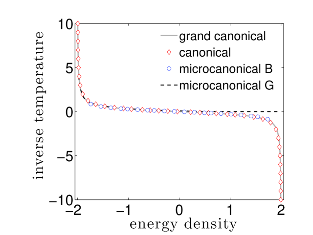
After Eq. (54), the condition imposes the constrain that can be satisfied in two cases: First, when (), ; Second, for () necessarily it results . Hence, in the latter case, we observe an inversion of population, namely with . For a given value of , the inverse temperature is a function of the energy density , in fact, by using Eq. (55) and (56) it is possible to getting rid of the chemical potential and is thus expressed as a function of . Figure 1 shows (gray) numerical results for vs for the case with sites where it is evident that positive and negative values of are allowed.
Ideal quantum gas: canonical description.
From the partition function (52) it is possible to compute the average of the energy density as a function of . We have done this numerically by generating all the microscopic configurations with , and by averaging the density energy (49) with respect to the canonical weight
as a function of . The resulting curve is shown in Fig. 1 (red).
Ideal quantum gas: microcanonical description.
In this case we have to calculate the density of states at energy density for a system with particles. We have obtained an approximation to by binning the energies of all the configurations with , which we generated as described above. In Fig. 1 we compare the inverse temperature vs the energy density (blue), obtained from the Boltzmann entropy and derived in the grand-canonical (gray) and in the canonical ensemble (red) for the case of . Already for this small system size it is evident the great agreement of between the case of Boltzmann definition and the corresponding relations derived in the grand-canonical and canonical ensembles. As we have recalled earlier, the Gibbs entropy yields a non-negative inverse temperature, irrespective of the energy density, . Now we show that the condition and cannot be satisfied in the grand canonical ensemble. Since for all , from Eq. (54) we deduce and, given that necessarily , and, in this manner implies . Furthermore, the single particle density levels have zero average (), therefore for this weighted average we get
which proves our assertion. As it is clearly shown in Fig. 1, (gray) derived with the grand canonical ensemble and (black) derived with the Gibbs entropy are absolutely irreconcilable in the region of .
Classical limit of the ideal quantum gas: grand canonical description.
For the classical model the grand canonical partition
| (57) |
yields
| (58) |
Hence the average energy density is
| (59) |
where the chemical potential is determined by the condition
| (60) |
and it is () in the region of positive temperatures, whereas for negative-temperature it results 999Notably, Eq. (58) is the classical limit () of the quantic result in Eq. (54).. Thus, one can derive the energy density
| (61) |
In the thermodynamic limit , we can consider the continuous limit for our system
| (62) |
Solving for the chemical potential we get
| (63) |
where is the particle density. Plugging Eq. (63) in the continuous limit of Eq. (59) we get
| (64) |
that plugged in (61) yields
| (65) |
in which is evident that and are smooth functions. Therefore, as expected, the energy density can be used to determine the inverse temperature and chemical potential of the system at equilibrium.
A few comments are worthwhile. The expression for the grand canonical partition function, Eq. (57), could suggest that the point corresponds to a singular point where some kind of phase transition takes place. This is not the case. Indeed it is easy to show from Eq. (63) that for , but and, hence, does not diverge at .
Classical limit of the ideal quantum gas: canonical description.
Classical limit of the ideal quantum gas: microcanonical description.
We want to calculate the Boltzmann entropy for the classical system introduced above. According to Boltzmann, the entropy depends on the density of states
| (70) |
through Eq. (5). By a direct calculation, in the case of a lattice of sites, one gets
| (71) |
where , the single particle energies are defined in (50), and
| (72) |
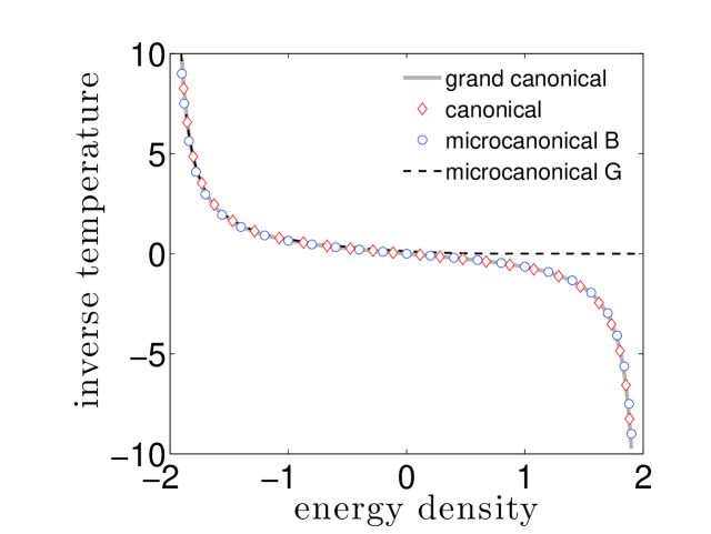
from which it is possible to derive by means the standard definition . Fig. 2 compares the inverse microcanonical temperature vs (blue) for a lattice of sites and one particle per site, Eq. (65) obtained in the grand canonical ensemble (gray) and the analogue relation derived in the canonical ensemble (red). Fig. 2 shows beyond a shadow of a doubt the agreement between the functions derived from the Boltzmann’s definition, and the one in the grand canonical ensemble. In particular they both predict negative temperatures in the domain of positive-energy densities. Furthermore from (72) we have derived from which it is possible to derive the inverse Gibbs temperature by means the standard definition . In Fig. 2 we show the curve (black) derived in such way. Also for the classical model, does not agree with the curves obtained in the grand canonical and canonical ensembles.
For the first system considered in this section, we have shown that derived within the canonical description agrees with derived within the Boltzmann microcanonical description. Furthermore, we have considered a second system, an ideal gas both in the classical and in the quantum case, and we have shown that derived within the grand canonical and canonical descriptions agree with the same quantity derived within a microcanonical description à la Boltzmann, whereas are irreconcilable with the analogues quantity derived using the Gibbs entropy. We have shown that, for these systems the ensemble equivalence holds true provided that the Boltzmann entropy is used within microcanonical ensemble. Furthermore, we have seen that for the classical case of the second system, the grand canonical approach gives an explicit form for , i.e. Eq. (65). In view of the clear agreement between the grand canonical and the microcanonical result, we can conclude
| (73) |
where does not depend on . Plugging and in the Eqs. (22) - (25), we deduce: First, is well defined within the whole range of value of , Second, for in , Third, in the thermodynamic limit is well defined only in the domain of corresponding to positive temperatures and it is infinity for . This fact has dramatic consequences about the thermodynamic consistency of Gibbs entropy, as we will show in Sec. 8.
In the light of these facts, it is evident that thermodynamics derived from Boltzmann entropy is perfectly consistent, both mathematically and thermodynamically, with the thermodynamics derived in the grand-canonical and canonical ensembles, whereas the thermodynamics derived from Gibbs entropy is inconsistent with that of these latter ensembles.
8 Equipartition theorem
While the Hamiltonian dynamics takes place on the phase-space hypersurface corresponding to a given value of the energy density (and possibly of the other conserved quantities), the Gibbs entropy requires measures involving all the energy level sets with density energy below such value. It is therefore not immediately clear how can be measured as an ensemble or time average. The usual answer to this question given by the supporters of the Gibbs entropy is to use the equipartition theorem. This can be cast into the form
| (74) |
where denotes any component of the set of dynamical coordinates and the angle brackets denote the standard microcanonical average. Nevertheless Eq. (74) is not valid exactly in the case of systems that admit negative temperature. For instance, in the case of system (51) reported in Sec. 7, in the region (corresponding to negative Boltzmann temperatures) the r.h.s. of Eq. (74) with is which is a well defined quantity for any system size . On the contrary, as we have proved above, l.h.s. goes to infinity as increases, therefore Eq. (74) cannot be satisfied. The reason of this failure of the equipartition theorem, in the case of systems that admit negative temperatures, stems from ignoring boundary terms in the derivation of Eq. (74). For instance, in the case of systems with bounded energy spectrum, like the systems admitting negative Boltzmann temperatures, the identity of Eq. (74) is no more valid and must be corrected with
| (75) |
that includes boundary terms. In fact, such terms in the case of systems with bounded energy spectrum (and/or bounded coordinates), can be not null, at variance with standard systems where yields .
In the case of standard systems, i.e. with unbounded energy spectrum, Eq. (74) holds, but in this case the thermodynamic quantities derived from the Gibbs entropy differ from those obtained with the Boltzmann’s definition of entropy for quantities which are irrelevant from the statistical point of view, since they vanish in the thermodynamic limit.
In the case of the classical model of lattice ideal gas (51), by a direct calculation one can show that even in the canonical ensemble the equipartition theorem does not have the celebrated form of Eq. (74), with the microcanonical average replaced by the canonical one, but the following
| (76) |
where, with a glance at (68), the dependence on the mode index is evident. For the same system (75) is
| (77) |
Therefore, for systems with bounded energy spectrum, the equipartition theorem assumes an unexpected mathematical form which is perfectly defined within the Boltzmann description. On the contrary, identity (74) becomes meaningless for this class of systems proving in such a way the flimsiness of Gibbs microcanonical thermodynamics.
We conclude that the identity (74) cannot be advocated as proof in favour of Gibbs entropy, since it is not valid in the case of systems where Gibbs and Boltzmann disagree. The correct identity (75), shows that there is not equipartition. Furthermore, since Eq. (74) is not valid, it cannot used to measure the Gibbs temperature as a microcanonical average.
9 Measuring temperature
Making a temperature measurement on a system brings about, inevitably, a contact between the system and a second “small system”. Especially in the present context a particular care has to be employed when we choose a second calibrated system (thermometer) to attach to the first one (sample) in order to determine the temperature of the latter. The thermometer has to detect the sample temperature without destroying its equilibrium. This means that a thermometer capable of sustaining negative temperatures must be employed with a sample admitting negative temperatures. Indeed, the whole system, obtained by glueing together a “small” system with unbounded energies, like an harmonic oscillator, to the sample would be a system with unbounded energies, that is without negative temperatures. In other words, a “small” system with unbounded energies will be able to detect only the positive temperatures. This aspect that appears as a good reasoning, has been diffusely discussed by Ramsey in its paper [5] even if several authors [19, 27] seem to have missed this point.
Furthermore, it makes sense to ask oneself if (and how) two systems admitting negative temperatures reach equilibrium when joined together at an initial different temperature.
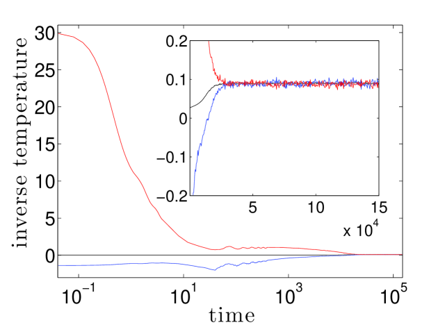
In particular, a relevant question is whether the two joined systems reach eventually the same inverse temperature and if, or not, this latter is intermediate respect to the initial inverse temperatures of the two systems as we expect from statistical mechanics of positive temperatures [18]. In order to directly verify if the Boltzmann temperature complies with this requisite, we have simulated an experiment in which two different systems that admit negative temperatures, at different initial temperatures, are brought to contact with each other. Thus we have considered two systems described by the following Hamiltonians
| (78) |
where, for each system, the indices and run over a two-dimensional lattice and is the adjacency matrix that describes the nearest-neighbour interaction in two spatial dimensions. In (78) we have added to a kinetic a term similar that of Hamiltonian (51), an onsite nonlinear potential, in order to make the systems not integrable. Note, that also with the addition of this latter term, the system admits negative temperatures. We started with the two systems isolated with each other. In our simulations we have prepared the initial configuration of equilibrium for the two systems at different temperatures (, ), by means of a long time integration of the equations of motion of the two separated systems. The inverse temperatures (), have been measured with Eq. (14), that descends from the Boltzmann entropy. The two systems of sites have been joined to form a single lattice. In the simulation reported in Fig. 3 we set and , and . We integrated the equations of motion of the whole system. In Fig. 3 we report the inverse temperature for the whole system (black), subsystem (blue) and subsystem (red). As it was expected, we observe that the inverse temperature of the whole system, after a short transient, reaches an asymptotic value intermediate between the initial values of the inverse temperatures of the two original systems. Also, the inverse temperatures of the two subsystems approach the value of along the time. Furthermore, this value remains stable on long time scales. For detail about these numerical results we refer to [43], where we have presente analytical and numerical evidence that Boltzmann microcanonical entropy allows the description of phase transitions occurring at (negative Boltzmann temperatures) high energy densities, at variance with Gibbs temperature.
It is worth remarking that, whereas this process of thermalization is well explained with the Boltzmann temperature, we cannot say the same for the inverse temperature of Gibbs for which it is with and .
Finally we have verified that, irrespective of the sign of the temperature, a large lattice (that realizes a microcanonical ensemble) acts as a thermostat for a small sublattice (that realizes a grand canonical ensemble) and that the temperatures measures for the two systems agree, thus confirming the equivalence between the the microcanonical and the grand canonical ensemble.
10 Final remarks
We have addressed the question of the right definition of microcanonical entropy.
For systems for which the equivalence of the statistical ensembles is verified we have shown that the correct map between the canonical average of the energy (also for systems with one or more conserved quantities) and the Lagrangian parameter is that descending from the Boltzmann entropy. Moreover, we have concluded that the only consistent definition for the microcanonical entropy is that of Boltzmann. In fact, while for standard systems both these entropies lead to equivalent thermodynamic results in the thermodynamic limit [36], in the case of systems with bounded energy spectrum, negative Boltzmann temperatures are admitted, and the two microcanonical entropies lead to irreconciliable results. In particular, when the latter circumstance is verified, the inverse temperature derived by the Gibbs entropy coincides with the one of Boltzmann within the region of energy density where the latter is positive, and is identically null where the Boltzmann temperature is negative. In this way, it could happen that in correspondence of the energies where changes sign, is not a differentiable function of . But this conflicts with the fact that the canonical and grand canonical partition functions are smooth functions of in correspondence of such points. On the contrary, is a smooth function of , and no consistence issue of this kind arises for Boltzmann entropy.
For a general system, we have proved that: i) the Boltzmann entropy is thermostatistically consistent; ii) the Eq. (27), that has been adduced as thermostatistical self-consistency condition for entropy [19], actually is not a fundamental condition for the microcanonical entropy; iii) the Gibbs entropy is inconsistent with the thermostatistical condition that relates the generalized pressure and the free energy.
For all these reasons we conclude that the correct definition for the microcanonical entropy is the one of Boltzmann.
Acknowledgments
We are grateful to J. Dunkel, S. Hilbert, P. Hänggi and M. Campisi for sharing with us their different view on the Boltzmann and Gibbs entropy. We thank M. Gabbrielli for useful discussions.
References
References
- Onsager [1949] L. Onsager, supp. to Nuovo Cimento 6 (1949) 279–287.
- Pound [1951] R. V. Pound, Phys. Rev. 81 (1951) 156–156.
- Purcell and Pound [1951] E. M. Purcell, R. V. Pound, Phys. Rev. 81 (1951) 279–280.
- Ramsey and Pound [1951] N. F. Ramsey, R. V. Pound, Phys. Rev. 81 (1951) 278–279.
- Ramsey [1956] N. F. Ramsey, Phys. Rev. 103 (1956) 20–28.
- Kittel and Kroemer [1980] C. Kittel, H. Kroemer, Thermal physics, W.H. Freeman and Company, 1980, 2nd ed, 1980.
- Landau and Lifschitz [1980] L. Landau, E. Lifschitz, Statistical physics, Pergamon Press Ltd., 1980, 3rd ed, 1980.
- Jaynes [1965] E. T. Jaynes, American Journal of Physics 33 (1965) 391–398.
- Hertz [1910] P. Hertz, Ann. Phys. 338 (1910) 225.
- Einstein [1911] A. Einstein, Ann. Phys. 339 (1911) 175.
- Schlüter [1948] A. Schlüter, Z. Naturforschg. 3a (1948) 350.
- Berdichevsky et al. [1991] V. Berdichevsky, I. Kunin, F. Hussain, Phys. Rev. A 43 (1991) 2050–2051.
- Münster [1969] A. Münster, Statistical Thermodynamics, Springer Berlin, 1969.
- Pearson et al. [1985] E. M. Pearson, T. Halicioglu, W. A. Tiller, Phys. Rev. A 32 (1985) 3030–3039.
- Campisi [2005] M. Campisi, Studies in History and Philosophy of Science Part B: Studies in History and Philosophy of Modern Physics 36 (2005) 275 – 290.
- Adib [2004] A. Adib, Journal of Statistical Physics 117 (2004) 581.
- Lavis [2005] D. Lavis, Studies in History and Philosophy of Science Part B: Studies in History and Philosophy of Modern Physics 36 (2005) 245 – 273.
- Huang [1987] K. Huang, Statistical Mechanics, 2 ed., John Wiley & Sons, 1987.
- Dunkel and Hilbert [2013] J. Dunkel, S. Hilbert, Nature Physics 10 (2013) 67–72.
- Hilbert et al. [2014] S. Hilbert, P. Hänggi, J. Dunkel, Phys. Rev. E 90 (2014) 062116.
- Hänggi et al. [2016] P. Hänggi, S. Hilbert, J. Dunkel, Phil. Trans. Roy. Soc. A 374 (2016) 20150039.
- Sokolov [2014] I. M. Sokolov, Nat Phys 10 (2014) 7–8.
- Dunkel and Hilbert [2014a] J. Dunkel, S. Hilbert, arXiv:1403.6058 (2014a).
- Dunkel and Hilbert [2014b] J. Dunkel, S. Hilbert, arXiv:1408.5392 (2014b).
- Campisi [2015] M. Campisi, Phys. Rev. E 91 (2015) 052147.
- Campisi [2016] M. Campisi, Phys. Rev. E 93 (2016) 039901.
- Romero-Rochín [2013] V. Romero-Rochín, Phys. Rev. E 88 (2013) 022144.
- Treumann and Baumjohann [2014a] R. A. Treumann, W. Baumjohann, arXiv:1406.6639 (2014a).
- Treumann and Baumjohann [2014b] R. A. Treumann, W. Baumjohann, Frontiers in Physics 2 (2014b).
- Vilar and Rubi [2014] J. M. G. Vilar, J. M. Rubi, The Journal of Chemical Physics 140 (2014).
- Frenkel and Warren [2015] D. Frenkel, P. B. Warren, American Journal of Physics 83 (2015) 163–170.
- Schneider et al. [2014] U. Schneider, S. Mandt, A. Rapp, S. Braun, H. Weimer, I. Bloch, A. Rosch, arXiv:1407.4127 (2014).
- Wang [2015] J.-S. Wang, arXiv:1507.02022 (2015).
- Swendsen and Wang [2016] R. H. Swendsen, J.-S. Wang, Physica A: Statistical Mechanics and its Applications 453 (2016) 24 – 34.
- Müller and Müller [2009] I. Müller, W. H. Müller, Fundamentals of Thermodynamics and Applications, Springer-Verlag, Berlin Heidelberg, 2009.
- Toda et al. [1992] M. Toda, R. Kubo, N. Saito, Statistical Physics I. Equilibrium Statistical Mechanics, Springer Verlag, Berlin, 1992.
- Mosk [2005] A. P. Mosk, Phys. Rev. Lett. 95 (2005) 040403.
- Rapp et al. [2010] A. Rapp, S. Mandt, A. Rosch, Phys. Rev. Lett. 105 (2010) 220405.
- Iubini et al. [2013] S. Iubini, R. Franzosi, R. Livi, G.-L. Oppo, A. Politi, New Journal of Physics 15 (2013) 023032.
- Braun et al. [2013] S. Braun, J. P. Ronzheimer, M. Schreiber, S. S. Hodgman, T. Rom, I. Bloch, U. Schneider, Science 339 (2013) 52–5.
- Poulter [2016] J. Poulter, Phys. Rev. E 93 (2016) 032149.
- Cerino et al. [2015] L. Cerino, A. Puglisi, A. Vulpiani, Journal of Statistical Mechanics: Theory and Experiment 2015 (2015) P12002.
- Buonsante et al. [2015] P. Buonsante, R. Franzosi, A. Smerzi, arXiv:1506.01933 (2015).
- Swendsen and Wang [2015] R. H. Swendsen, J.-S. Wang, Phys. Rev. E 92 (2015) 020103.
- Swendsen [2015] R. H. Swendsen, Phys. Rev. E 92 (2015) 052110.
- Matty et al. [2016] M. Matty, L. Lancaster, W. Griffin, R. Swendsen, arXiv:1511.02830 (2016).
- Khinchin [1949] A. Khinchin, Mathematical Foundations of Statistical Mechanics, Dover Publications, 1949.
- Berdichevsky [1988] V. L. Berdichevsky, J. Appl. Math. Mech. (PMM) 52 (1988) 738 – 746.
- Rugh [1997] H. H. Rugh, Phys. Rev. Lett. 78 (1997) 772–774.
- Franzosi [2011] R. Franzosi, Journal of Statistical Physics 143 (2011) 824–830.
- Franzosi [2012] R. Franzosi, Phys. Rev. E 85 (2012) 050101.
- Federer [1969] H. Federer, Geometric Measure Theory, Springer-Verlag, New York Inc., 1969.
- Laurence [1989] P. Laurence, Zeitschrift für angewandte Mathematik und Physik ZAMP 40 (1989) 258–284.
- Gallavotti [1999] G. Gallavotti, Statistical Mechanics: A Short Treatise, Springer, 1999.
- Ruelle [1989] D. Ruelle, Statistical mechanics : rigorous results, Advanced book classics, Addison-Wesley, 1989.
- Hüller [1994] A. Hüller, Z. Phys. B 96 (1994) 401 – 405.
- Gross [2001] D. Gross, Microcanonical Thermodynamics: Phase Transitions in “small” Systems, World Scientific, 2001.