Spin Polarized versus Chiral Condensate in Quark Matter
at Finite Temperature and Density

Abstract

It is shown that the spin polarized condensate appears in quark matter at high baryon density and low temperature due to the tensor-type four-point interaction in the Nambu-Jona-Lasinio-type model as a low energy effective theory of quantum chromodynamics. It is indicated within this low energy effective model that the chiral symmetry is broken again by the spin polarized condensate as increasing the quark number density, while the chiral symmetry restoration occurs in which the chiral condensate disappears at a certain density.

1 Introduction

One of recent interests in the physics of the strong interaction, namely, in the physics governed by quantum chromodynamics (QCD), may be to clarify the structure of the phase diagram on the plane with respect to baryon chemical potential and temperature [1]. In the region of finite temperature and zero baryon chemical potential, lattice QCD simulation works and reliable calculations based on the first principles are performed until now. However, in the region of the low temperature and the finite baryon chemical potential, the possibility for various phases has been indicated such as the color superconducting phase [2, 3, 4], quarkyionic phase [5], inhomogeneous chiral condensed phase [6, 7, 8] and so on.

In heavy-ion collision experiments such as the relativistic heavy-ion collider (RHIC) experiment, it is believed that quark-gluon phase is realized. Also, in the large hadron collider (LHC) experiment, it is expected that more extreme states of QCD with finite temperature and density and/or a strong magnetic field may be created in quark-gluon phase. It is interesting to understand what phases arise under extreme conditions. The quark-gluon phase under extreme conditions may be realized in the inner core of compact stars such as neutron stars, magnetars and quark stars if they exist. Therefore, the investigation of quark matter at low temperature and high density is also important to understand the compact star objects.

In our previous papers, it has been shown that a spin polarized phase may appear and be realized instead of the color superconducting phase in both the cases of two- [9] or three-flavor [10] in the region with finite quark chemical potential at zero temperature. It is further interesting to investigate possible phases in the region with high density and low temperature from a viewpoint of physics of compact stars, especially, the structure of inner core of the compact stars. It has also been shown in our recent work [11] that there is a possibility of the existence of a strong magnetic field on the surface of compact stars if there exists a quark spin polarized phase, which leads to the spontaneous magnetization of quark matter due to anomalous magnetic moment of quark, while only symmetric quark matter has been considered. If the spin polarization really leads to the spontaneous magnetization in the mechanism developed in the previous paper [11], it is a possible candidate for the origin of the strong magnetic field in so-called magnetar. [12, 13, 14]

In this paper succeeding to Refs.oursPTP and oursPTEP1, a possibility of the quark spin polarized phase is investigated in the region of finite quark chemical potential and finite temperature by using the Nambu-Lona-Lasinio (NJL) model [16, 17, 18] with the tensor-type four-point interaction between quarks [19], instead of the pseudovector-type four-point interaction [20, 21]. As for the tensor-type four-point interaction, this interaction term was also introduced to investigate the meson spectroscopy, especially, for vector and axial-vector mesons [22]. As another application, the dynamic properties of vector mesons were investigated in the extended NJL model including the tensor-type interaction [23]. Also, the chiral condensate and the quark spin polarization, namely, the tensor condensate, are considered simultaneously in the case with only one flavor instead of the color superconductor [24].

This paper is organized as follows: In the next section, the recapitulation of the NJL model with the tensor-type four-point interaction between quarks is given and in this model the chiral condensate and quark spin polarized condensate are considered simultaneously. In §3, the thermodynamic potential at zero temperature is introduced under the mean field approximation. In §4, the thermodynamic potential at finite temperature and density is given and derived. A derivation of the thermodynamic potential at zero temperature from that at finite temperature is given in Appendix A. Also, the effective potential is evaluated in Appendix B. In Appendix C, the analytic calculation for the thermodynamic potential is presented. In §5, the numerical results are given through the calculation of the thermodynamic potential under various temperatures and quark chemical potentials. The results are summarized in the phase diagram on the plane with respect to the quark chemical potential and temperature, in which the possible phases, the position of phase boundary and the order of the phase transition are shown, apart from the color superconducting phase. In Appendix D, an idea introducing the tensor-type four-point interaction between quarks, which plays an essential role in this paper, is given from a viewpoint of two-gluon exchange process in QCD. The last section is devoted to a summary and concluding remarks.

2 NJL model with a tensor-type four-point interaction

Let us consider the NJL-model Lagrangian density with a tensor-type four-point interaction. The Lagrangian density with $su(2)$-flavor symmetry can be expressed as

$$\mathcal{L}=\mathcal{L}_{0}+\mathcal{L}_{\text{S}}+\mathcal{L}_{\text{T}},$$ (2.1)

$$\mathcal{L}_{0}=\bar{\psi}(i\gamma^{\mu}\partial_{\mu}-m_{0})\psi,$$ (2.2)

$$\mathcal{L}_{\text{S}}=G_{\text{S}}\left\{(\bar{\psi}\psi)^{2}+(\bar{\psi}i\gamma^{5}\vec{\tau}\psi)^{2}\right\},$$ (2.3)

$$\mathcal{L}_{\text{T}}=-\frac{G_{\text{T}}}{4}\left\{(\bar{\psi}\gamma^{\mu}\gamma^{\nu}\vec{\tau}\psi)\cdot(\bar{\psi}\gamma_{\mu}\gamma_{\nu}\vec{\tau}\psi)+(\bar{\psi}i\gamma^{5}\gamma^{\mu}\gamma^{\nu}\psi)(\bar{\psi}i\gamma^{5}\gamma_{\mu}\gamma_{\nu}\psi)\right\},$$ (2.4)

where $m_{0}$ is a current quark mass for up and down quark and the components of $\vec{\tau}$ are the Pauli matrices for isospin. It is known that these current quark masses are slightly different for each flavor, but we have used the same value approximately. The first two terms, $\mathcal{L}_{0}+\mathcal{L}_{\text{S}}$, is the original NJL-model Lagrangian density. In this paper $\mathcal{L}_{\text{T}}$ is added into the model, according to the Fierz transform. Then, the spin matrix appears from $\mathcal{L}_{\text{T}}$ when $\mu=1$, $\nu=2$ or $\mu=2$, $\nu=1$ as follows:

$$\varSigma_{3}=-i\gamma^{1}\gamma^{2}=\begin{pmatrix}\sigma_{3}&0\\ 0&\sigma_{3}\end{pmatrix}.$$

Since we use the mean field approximation, then we get the mean field Lagrangian density as

$$\mathcal{L}_{\text{MFA}}= \bar{\psi}(i\gamma^{\mu}\partial_{\mu}-m_{0})\psi+G_{\text{S}}\left\{2\langle\bar{\psi}\psi\rangle(\bar{\psi}\psi)-\langle\bar{\psi}\psi\rangle^{2}\right\}$$

$$+\frac{G_{\text{T}}}{2}\left\{2\langle\bar{\psi}\varSigma_{3}\tau_{3}\psi\rangle(\bar{\psi}\varSigma_{3}\tau_{3}\psi)-\langle\bar{\psi}\varSigma_{3}\tau_{3}\psi\rangle^{2}\right\},$$ (2.5)

where $\langle\cdots\rangle$ means vacuum expectation value. Here $\tau_{3}$ is the third component of the Pauli matrix for isospin. When it operates on $\psi$ for up-quark (down-quark), the matrix changes into $1$ $(-1)$ as its eigenvalue. Thus we could safely express $\bar{\psi}\varSigma_{3}\tau_{3}\psi$ as follows:

$$\bar{\psi}\varSigma_{3}\tau_{3}\psi\rightarrow\bar{\psi}\varSigma_{3}\psi\tau_{f},$$

where $\tau_{f}=1$ $(-1)$ when $f=$ up-quark (down-quark). Let us define the following quantities:

$$F\equiv-G_{\text{T}}\langle\bar{\psi}\varSigma_{3}\psi\rangle,\,\qquad M\equiv-2G_{\text{S}}\langle\bar{\psi}\psi\rangle,\,\qquad M_{\text{q}}\equiv m_{0}+M.$$

$F$ and $M$ are especially important quantities, because if $F$ and/or $M$ are not equal to zero, then spin polarization and/or chiral condensation occur. Here, $M_{\text{q}}$ is just a constituent quark mass. Substituting these quantities into Eq.(2.5), we convert $\mathcal{L}_{\text{MFA}}$ into

$$\mathcal{L}_{\text{MFA}}=\bar{\psi}(i\gamma^{\mu}\partial_{\mu}-M_{\text{q}})\psi-F(\bar{\psi}\varSigma_{3}\psi)-\frac{M^{2}}{4G_{\text{S}}}-\frac{F^{2}}{2G_{\text{T}}}.$$ (2.6)

Let us switch from Lagrangian formalism to Hamiltonian formalism by Legendre transformation. First we must obtain the canonical momentum $\pi_{\alpha}$, $\pi_{\alpha}={\partial\mathcal{L}_{\text{MFA}}}/{\partial\dot{\psi_{\alpha}}}=i\psi_{\alpha}^{\dagger}$, where $\alpha$ means an index for spinor and isospin. We, therefore, get the Hamiltonian density:

$$\mathcal{H}_{\text{MFA}} =\pi_{\alpha}\dot{\psi_{\alpha}}-\mathcal{L}_{\text{MFA}}$$

$$=\bar{\psi}(-i\vec{\gamma}\cdot\vec{\nabla}+M_{\text{q}})\psi+F(\bar{\psi}\varSigma_{3}\psi)+\frac{M^{2}}{4G_{\text{S}}}+\frac{F^{2}}{2G_{\text{T}}}.$$ (2.7)

Thus, the Hamiltonian is expressed as

$$H_{\text{MFA}}=\int d^{3}x\,\psi^{\dagger}\gamma^{0}(-i\vec{\gamma}\cdot\vec{\nabla}+M_{\text{q}}+F\varSigma_{3})\psi+V\frac{M^{2}}{4G_{\text{S}}}+V\frac{F^{2}}{2G_{\text{T}}},$$

where V is the volume of this system. We transform $\psi(x)$ by the Fourier transformation as $\psi(x)=\int{d^{3}p}/{(2\pi)^{3}}\cdot\tilde{\psi}(p)e^{i{\vec{p}}\cdot{\vec{x}}}.$ Substituting it into $H_{\text{MFA}}$, we obtain

$$H_{\text{MFA}}=\int\frac{d^{3}p}{(2\pi)^{3}}\tilde{\psi}^{\dagger}\gamma^{0}(\vec{\gamma}\cdot\vec{p}+M_{\text{q}}+F\varSigma_{3})\tilde{\psi}+V\frac{M^{2}}{4G_{\text{S}}}+V\frac{F^{2}}{2G_{\text{T}}}.$$ (2.8)

What we must do is to diagonalize $H_{\text{MFA}}$. Non diagonal terms are

$$h_{\text{MFA}} \equiv\gamma^{0}(\vec{\gamma}\cdot\vec{p}+M_{\text{q}}+F\varSigma_{3})$$

$$=\begin{pmatrix}F\sigma_{3}+M_{\text{q}}&\vec{p}\cdot\vec{\sigma}\\ \vec{p}\cdot\vec{\sigma}&-F\sigma_{3}-M_{\text{q}}\end{pmatrix}$$

$$=\begin{pmatrix}F+M_{\text{q}}&0&p_{3}&p_{1}-ip_{2}\\ 0&-F+M_{\text{q}}&p_{1}+ip_{2}&-p_{3}\\ p_{3}&p_{1}-ip_{2}&-F-M_{\text{q}}&0\\ p_{1}+ip_{2}&-p_{3}&0&F-M_{\text{q}}\end{pmatrix}.$$

Since $h_{\text{MFA}}$ is a hermitian matrix, it is diagonalized by a unitary matrix. The eigenvalues are obtained as

$$\pm E^{(\eta)}_{\vec{p}}=\pm\sqrt{p_{3}^{2}+\left(\sqrt{p_{1}^{2}+p_{2}^{2}+M_{\text{q}}^{2}}+\eta F\right)^{2}},$$ (2.9)

where $\eta=\pm 1$.

3 Thermodynamic potential at zero temperature

Next, we introduce a quark chemical potential $\mu$ and a number density operator $\mathcal{N}$ in order to discuss on a finite density system at zero temperature. The thermodynamic potential is defined as follows:

$$\varPhi=\mathcal{H}_{\text{MFA}}-\mu\mathcal{N}.$$ (3.1)

The next step is to calculate the expectation value. Since we consider the zero-temperature system in this section, the system that quasi-particles degenerate is treated. Hence, we must sum over momenta from zero to the single-quasi-particle energy equal to the chemical potential. Sandwiching with a “bra” and “ket”, we obtain

$$\varPhi =\frac{1}{V}\langle\text{F.D.}|\left(H_{\text{MFA}}-\mu\int d^{3}x\,\mathcal{N}\right)|\text{F.D.}\rangle$$

$$=\frac{1}{V}\sum^{E^{(\eta)}_{\vec{p}}\leq\mu,\vec{p}^{2}\leq\varLambda^{2}}_{\vec{p},\eta,\tau,\alpha}\left(E^{(\eta)}_{\vec{p}}-\mu\right)+\frac{M^{2}}{4G_{\text{S}}}+\frac{F^{2}}{2G_{\text{T}}},$$

where $|\text{F.D.}\rangle$ means the degenerate Fermi gas constituted by quasi-particles and $\varLambda$ is a three-momentum cutoff parameter for the integration over momenta. Here, $\tau$ and $\alpha$ are indeces for isospin and quark color, respectively. The upper limit of integration is imposed by two conditions, which are $E^{(\eta)}_{\vec{p}}\leq\mu$ and $\vec{p}^{2}\leq\varLambda^{2}$. We would like to discuss spin polarization and chiral condensate simultaneously. However, the above expression does not have the contribution from Dirac sea. Since chiral condensate occurs by the effect of Dirac sea, we must add its contribution. Thus, we get

$$\varPhi(M,F,\mu)=\frac{1}{V}\sum^{E^{(\eta)}_{\vec{p}}\leq\mu,\vec{p}^{2}\leq\varLambda^{2}}_{\vec{p},\eta,\tau,\alpha}\left(E^{(\eta)}_{\vec{p}}-\mu\right)-\frac{1}{V}\sum^{\vec{p}^{2}\leq\varLambda^{2}}_{\vec{p},\eta,\tau,\alpha}E^{(\eta)}_{\vec{p}}+\frac{M^{2}}{4G_{\text{S}}}+\frac{F^{2}}{2G_{\text{T}}},$$ (3.2)

where, the second term represents the contribution from the Dirac sea (negative energy sea). We change the sum $\frac{1}{V}\sum_{\vec{p}}$ into the integration $\int\frac{d^{3}p}{(2\pi)^{3}}$. Then, the thermodynamic potential can be expressed as

$$\varPhi(M,F,\mu)=\varPhi_{1}+\varPhi_{2}+\varPhi_{3}+\varPhi_{4},$$ (3.3)

where,

$$\varPhi_{1}(F,M,\mu)=\sum_{\tau,\alpha} \int_{\varGamma_{1}}\frac{d^{3}p}{(2\pi)^{3}}\left\{\sqrt{p_{3}^{2}+(\sqrt{p_{1}^{2}+p_{2}^{2}+M_{\text{q}}^{2}}+F)^{2}}-\mu\right\},$$

$$\varGamma_{1}=\left\{E^{(+1)}_{\vec{p}}\leq\mu,\,\vec{p}^{2}\leq\varLambda^{2}\right\}$$ (3.4)

$$\varPhi_{2}(M,F,\mu)=\sum_{\tau,\alpha} \int_{\varGamma_{2}}\frac{d^{3}p}{(2\pi)^{3}}\left\{\sqrt{p_{3}^{2}+(\sqrt{p_{1}^{2}+p_{2}^{2}+M_{\text{q}}^{2}}-F)^{2}}-\mu\right\},$$

$$\varGamma_{2}=\left\{E^{(-1)}_{\vec{p}}\leq\mu,\,\vec{p}^{2}\leq\varLambda^{2}\right\}$$ (3.5)

$$\varPhi_{3}(M,F,\mu)=-\sum_{\eta,\tau,\alpha} \int_{\varGamma_{3}}\frac{d^{3}p}{(2\pi)^{3}}\sqrt{p_{3}^{2}+(\sqrt{p_{1}^{2}+p_{2}^{2}+M_{\text{q}}^{2}}+\eta F)^{2}},\ \ \$$

$$\varGamma_{3}=\left\{\vec{p}^{2}\leq\varLambda^{2}\right\}\quad$$ (3.6)

$$\varPhi_{4}(M,F,\mu)=\frac{M^{2}}{4G_{\text{S}}}+\frac{F^{2}}{2G_{\text{T}}}.\qquad\qquad\qquad\qquad\qquad\qquad\qquad\qquad$$ (3.7)

Here, $\varPhi_{i}$ $(i=1,2,3,4)$ means, respectively, the contribution from positive energy for $\eta=+1$, from positive energy for $\eta=-1$, from vacuum and the mean field contribution, respectively. $\varGamma_{i}$ $(i=1,2,3)$ is the domain of integration over momenta. Since these integrands do not depend on $\tau$ or $\alpha$, the summations over $\tau$ and $\alpha$ give factors $2$ and $3$, respectively.

4 Thermodynamic potential at finite temperature and density

We have discussed the thermodynamic potential at zero temperature in the previous section. In this section let us consider the thermodynamic potential at finite temperature. We define a thermodynamic potential at finite temperature, $\varOmega(M,F,\mu,T)$, as follows:

$$\varOmega(M,F,\mu,T)\equiv\mathcal{H}^{\prime}_{\text{MFA}}-\mu(\mathcal{N}_{\text{P}}-\mathcal{N}_{\text{AP}})+V_{\text{vacuum}}-TS,$$ (4.1)

$$\mathcal{H}^{\prime}_{\text{MFA}}\equiv\sum_{\vec{p},\eta,\tau,\alpha}E^{(\eta)}_{\vec{p}}\left(n^{(\eta)}_{\vec{p}}+\bar{n}^{(\eta)}_{\vec{p}}\right)+\frac{M^{2}}{4G_{\text{S}}}+\frac{F^{2}}{2G_{\text{T}}},$$

$$\mathcal{N}_{\text{P}}\equiv\sum_{\vec{p},\eta,\tau,\alpha}n^{(\eta)}_{\vec{p}},\,\qquad\mathcal{N}_{\text{AP}}\equiv\sum_{\vec{p},\eta,\tau,\alpha}\bar{n}^{(\eta)}_{\vec{p}},$$

$$n^{(\eta)}_{\vec{p}}=\frac{1}{1+\exp\left((E^{(\eta)}_{\vec{p}}-\mu)/T\right)},\,\qquad\bar{n}^{(\eta)}_{\vec{p}}=\frac{1}{1+\exp\left((E^{(\eta)}_{\vec{p}}+\mu)/T\right)},$$

$$V_{\text{vacuum}}\equiv-\sum_{\vec{p},\eta,\tau,\alpha}E^{(\eta)}_{\vec{p}},$$

where $T$ means temperature of the system, $n^{(\eta)}_{\vec{p}}$ and $\bar{n}^{(\eta)}_{\vec{p}}$ are the distribution functions for particle and anti-particle, respectively. The entropy $S$ is given as follows:

$$S =-\sum_{\vec{p},\eta,\tau,\alpha}\biggl{\{}n^{(\eta)}_{\vec{p}}\log n^{(\eta)}_{\vec{p}}+(1-n^{(\eta)}_{\vec{p}})\log(1-n^{(\eta)}_{\vec{p}})$$

$$\qquad\qquad\quad+\bar{n}^{(\eta)}_{\vec{p}}\log\bar{n}^{(\eta)}_{\vec{p}}+(1-\bar{n}^{(\eta)}_{\vec{p}})\log(1-\bar{n}^{(\eta)}_{\vec{p}})\biggr{\}}.$$

Using the following identities

$$n^{(\eta)}_{\vec{p}}\log n^{(\eta)}_{\vec{p}}=-n^{(\eta)}_{\vec{p}}\times\frac{E^{(\eta)}_{\vec{p}}-\mu}{T}-n^{(\eta)}_{\vec{p}}\log(1-n^{(\eta)}_{\vec{p}}),$$

$$\bar{n}^{(\eta)}_{\vec{p}}\log\bar{n}^{(\eta)}_{\vec{p}}=-\bar{n}^{(\eta)}_{\vec{p}}\times\frac{E^{(\eta)}_{\vec{p}}+\mu}{T}-\bar{n}^{(\eta)}_{\vec{p}}\log(1-\bar{n}^{(\eta)}_{\vec{p}}),$$

the above $\varOmega$ can be recast into

$$\varOmega =-\sum_{\vec{p},\eta,\tau,\alpha}\left\{E^{(\eta)}_{\vec{p}}+T\log\left(1+\exp\left(-\frac{E^{(\eta)}_{\vec{p}}-\mu}{T}\right)\right)+T\log\left(1+\exp\left(-\frac{E^{(\eta)}_{\vec{p}}+\mu}{T}\right)\right)\right\}$$

$$\ \ +\frac{M^{2}}{4G_{\text{S}}}+\frac{F^{2}}{2G_{\text{T}}}.$$

Let us change the summation over momenta into integration, and then let us introduce polar coordinates, $p_{1}=p_{T}\cos\theta,\,p_{2}=p_{T}\sin\theta$, so as to integrate. The domain of integration is obtained as follows:

$$-\sqrt{\varLambda^{2}-p_{T}^{2}}\leq p_{3}\leq\sqrt{\varLambda^{2}-p_{T}^{2}},\,\qquad 0\leq p_{T}\leq\varLambda.$$

After integrating over $\theta$, and summing over $\tau$ and $\alpha$, we get the final form:

$$\varOmega(M,F,\mu,T) =-\frac{3}{\pi^{2}}\sum_{\eta}\int_{0}^{\varLambda}dp_{T}\int_{0}^{\sqrt{\varLambda^{2}-p_{T}^{2}}}dp_{3}\,p_{T}$$

$$\qquad\qquad\times\left\{E^{(\eta)}_{\vec{p}}+T\log\left(1+\exp\left(-\frac{E^{(\eta)}_{\vec{p}}-\mu}{T}\right)\right)\right.$$

$$\qquad\qquad\qquad\left.+T\log\left(1+\exp\left(-\frac{E^{(\eta)}_{\vec{p}}+\mu}{T}\right)\right)\right\}$$

$$+\frac{M^{2}}{4G_{\text{S}}}+\frac{F^{2}}{2G_{\text{T}}}.$$ (4.2)

Table 1: Parameter set

$\varLambda$/GeV	$m_{0}$/GeV	$G_{\text{S}}$/GeV-2	$G_{\text{T}}$/GeV-2
0.631	0.0	5.5	11.0

5 Numerical results and discussions

In this section we would like to discuss the thermodynamic potential at zero/finite temperature numerically. In order to evaluate it we use the three-momentum cutoff parameter and coupling constants in Table 1. Here, we adopt the strength of tensor interaction $G_{\rm T}$ as a rather small value compared with the one used in our previous paper. The reason why we take $G_{\rm T}$ as a rather small value 11.0 GeV is that the vacuum polarization, namely the contribution of the negative energy sea, is taken into account. A detailed discussion of this effect has already been given in appendix B in [15]. Here, in this section, we show numerical results in the case of the chiral limit, $m_{0}=0.0$.

5.1 Thermodynamic potential at zero temperature

Let us discuss the thermodynamic potential at zero temperature. First we consider the chiral condensate $M$ and the spin polarization $F$ separately.

Figure 1 shows the thermodynamic potential in the special case where $F=0$. When the chemical potential has a value below $0.32$ GeV and above $0.35$ GeV, the thermodynamic potential has only one minimum. On the other hand, when $\mu=0.33\sim 0.34$ GeV, the thermodynamic potential has two local minima. This indicates that the phase transition to chiral condensate is of first order.

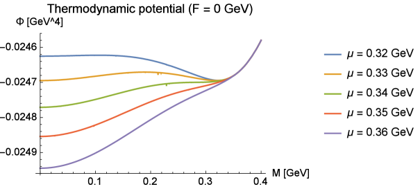
Figure 1: The thermodynamic potential with $F=0$ is depicted as a function of the constituent quark mass $M$ in various quark chemical potentials.

Figure 2 shows the thermodynamic potential for $M=0$. When the chemical potential is small, the spin polarized phase does not appear. However, the chemical potential $\mu$ has a value above $0.42$ GeV, the spin polarized phase appears. This figure shows that the phase transition to spin polarization is of the second order.

Next, let us consider $M$ and $F$ simultaneously. In Fig.3, the contour map for the thermodynamic potential is depicted with various quark chemical potentials. The horizontal and the vertical axes represent the constituent quark mass $M$ and the spin polarized condensate $F$, respectively. When $\mu$ varies from $0$ GeV to $0.32$ GeV, the chiral condensed phase arises. However, when $\mu$ reaches $0.35$ GeV, chiral symmetry is restored. If $\mu=0.43$ GeV, the spin polarized phase appears. From these contour maps, it indicates that two phases, the chiral condensed and the spin polarized phases, do not coexist.

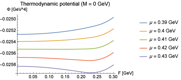
Figure 2: The thermodynamic potential with $M=0$ is depicted as a function of the spin polarized condensate $F$ in various quark chemical potentials.

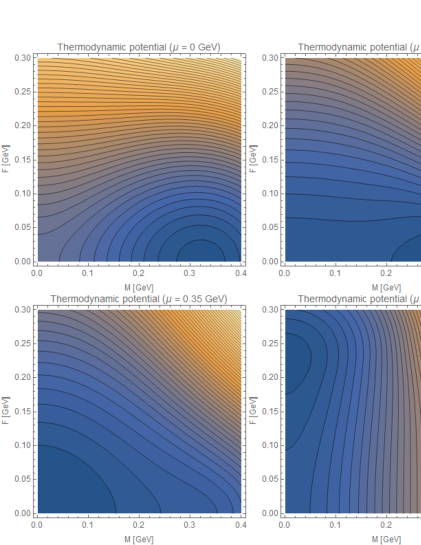
Figure 3: The contour map of the thermodynamic potential is depicted as a function of the constituent quark mass $M$ and the spin polarized condensate $F$ in various quark chemical potentials. The horizontal and vertical axes represent $M$ and $F$, respectively. As color becomes dark, the thermodynamic potential lowers.

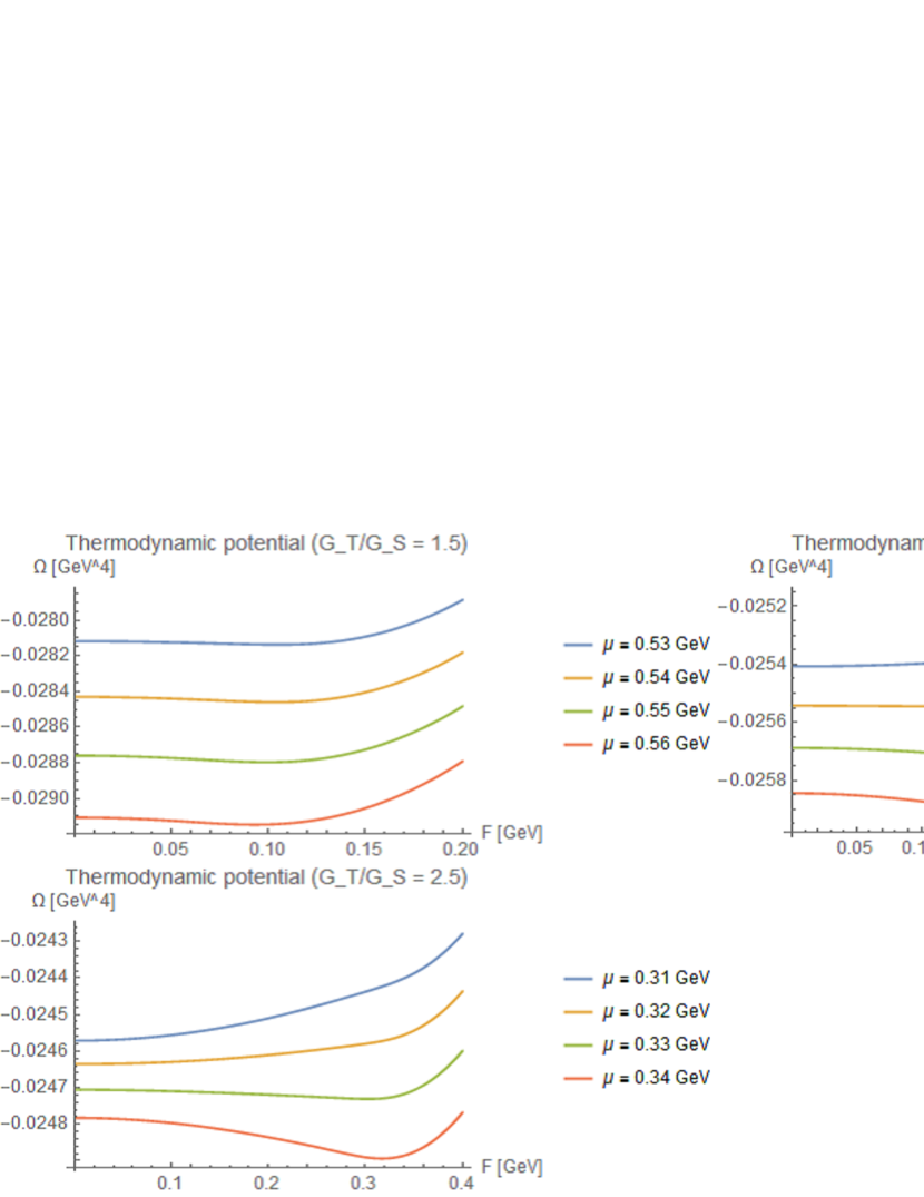
Figure 4: The thermodynamic potentials with $M=0$ and $T=0.01$ are depicted in the various ratios of $G_{T}/G_{S}$. The ratios $G_{T}/G_{S}=1.5,\,2$ and $2.5$ mean $G_{T}=8.25,\,11.0$ and $3.75\ \text{GeV}^{-2}$, respectively.

Here, two notes should be mentioned. One is about the effect of $G_{T}$, namely the coupling strength of the tensor-type interaction. As was already mentioned in the beginning of this section, a detailed discussion about $G_{T}$ has already been given in appendix B in [15]. However, let us demonstrate the effect of $G_{T}$ for the spin polarization. Figure 4 shows the thermodynamic potential with $M=0$ in various values of $G_{T}$, namely, $G_{T}/G_{S}=1,5,\ 2.0$ and $2.5$, respectively. As the coupling strength $G_{T}$ is increased, the critical chemical potential of phase transition is decreasing. For example, in the small value of $G_{T}$ such as $G_{T}/G_{S}=1.5$, the phase transition occurs around $\mu=0.54$ GeV. On the other hand, in the large $G_{T}$, $G_{T}/G_{S}=2.5$, the phase transition occurs around $\mu=0.33$ GeV. In this paper, we adopt a moderate value $G_{T}/G_{S}=2.0$ for discussions.

Another is about a reason why the spin polarization occurs at large chemical potential. At zero temperature, the spin polarized phase is actually realized in our model. It is easy to understand how the spin polarized phase appears. Neglecting the contribution of the chiral condensate, the energy $E$ of the system under consideration can be expressed by using the quark chemical potential as

$$E = \int^{\mu}\mu\frac{\partial N}{\partial\mu}d\mu+\frac{F^{2}}{2G_{T}}$$ (5.1)

$$= \mu N-\int Nd\mu+\frac{F^{2}}{2G_{T}}\ .$$

Thus, the thermodynamical potential $\Phi\ (=E-\mu N)$ is obtained as

$$\Phi = E-\mu N$$ (5.2)

$$= -\int Nd\mu+\frac{F^{2}}{2G_{T}}$$

$$= -\int d\mu\sum_{\eta,\tau,\alpha}\int\frac{d^{3}{\mib p}}{(2\pi)^{3}}\theta(\mu-E_{\vec{p}}^{(\eta)})+\frac{F^{2}}{2G_{T}}\ ,$$

where $\theta(x)$ represent the Heaviside step function. Let us consider the normal quark matter in which $F=0$. In this case, the above-derived thermodynamical potential can be calculated easily as

$$\Phi = -\frac{\mu^{4}}{2\pi^{2}}\ .$$ (5.3)

On the other hand, in the case $F\neq 0$, we can also calculate the thermodynamic potential analytically, which was presented in [19]. For simplicity, let us consider the case $F>\mu$. For $F>\mu$, $E_{\vec{p}}^{(+)}$ does not contributes to the three-momentum integration. In this case, by the existence of the theta function, the integration has a finite value in $E_{\vec{p}}^{(-)}\leq\mu$:

$$E_{\vec{p}}^{(-)}\equiv\sqrt{p_{3}^{2}+\left(F-\sqrt{p_{1}^{2}+p_{2}^{2}}\right)^{2}}\leq\mu.$$ (5.4)

In the case of equality in the above expression, this equality represents the formula of torus in which the major radius is $F$ and small radius is $\mu$. Thus, the Fermi surface has a form of torus. Therefore, the momentum integral $\int d^{3}{\bf p}\theta(\mu-E_{\vec{p}}^{(-)})$ means the volume of Fermi “torus”, where the volume gives $2\pi^{2}\mu^{2}F\ (=\pi\mu^{2}\cdot 2\pi F)$. Then, we obtain the thermodynamical potential in the large $\mu$ region as

$$\Phi = -\frac{3}{4\pi^{3}}\int^{\mu}d\mu 2\pi^{2}\mu^{2}F+\frac{F^{2}}{2G_{T}}$$ (5.5)

$$= -\frac{\mu^{3}F}{2\pi}+\frac{F^{2}}{2G_{T}}\ .$$

The “gap equation” for $F$ is derived from

$$\frac{\partial\Phi}{\partial F}=-\frac{\mu^{3}}{2\pi}+\frac{F}{G_{T}}=0\ ,\qquad{\rm thus,}\qquad F=\frac{G_{T}\mu^{3}}{2\pi}\ .$$ (5.6)

Inserting the above-derived $F$ into the thermodynamical potential, we finally obtain

$$\Phi=-\frac{G_{T}\mu^{6}}{8\pi^{2}}\ .$$ (5.7)

For small chemical potential, namely, at low quark number density, normal quark matter is realized because the thermodynamic potential has order $\mu^{4}$. On the other hand, for large chemical potential, namely, at high quark number density, the thermodynamical potential with the order of $\mu^{6}$ overcomes the normal quark matter with the order of $\mu^{4}$. It may be concluded that the appearance of the spin polarized phase is due to the effect of the volume of the phase space. Thus, at high density, the spin polarized phase is realized absolutely.

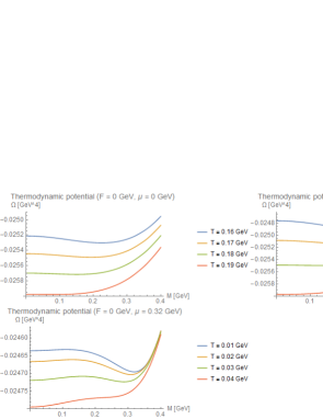
Figure 5: The thermodynamic potentials with $F=0$ are depicted in the various temperatures $T$ in the case with the chemical potential $\mu=0$, $0.2$ GeV and $0.32$ GeV, respectively. The horizontal and vertical axes represent the constituent quark mass $M$ and the thermodynamic potential $\varOmega(M,\mu,T)$, respectively.

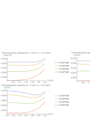
Figure 6: The thermodynamic potentials with $M=0$ are depicted in the various temperatures $T$ in the case with the chemical potential $\mu=0.41$ GeV, $0.42$ GeV and $0.44$ GeV, respectively. The horizontal and vertical axes represent the spin polarized condensate $F$ and the thermodynamic potential $\varOmega(F,\mu,T)$, respectively. .

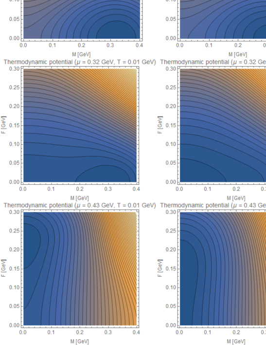
Figure 7: The contour maps of the thermodynamic potential are depicted as a function of the constituent quark mass $M$ and the spin polarized condensate $F$ with various quark chemical potentials and temperatures. The horizontal and vertical axes represent $M$ and $F$, respectively.

5.2 thermodynamic potential at finite temperature

Let us consider the thermodynamic potential at finite temperature. First, let us treat two cases without $M$ or $F$ separately. Figure 5 shows the thermodynamic potential at finite temperature for $F=0$. If temperature $T$ is not so high, the chiral condensed phase is realized. However, in high temperature region the chiral condensed phase disappears. It should be noted that, in the cases with $\mu=0$ GeV and $\mu=0.2$ GeV, the phase transition is of second order, while the phase transition is of first order in the case $\mu=0.32$ GeV.

Secondly, we discuss the case for $M=0$. In Fig. 6, it is shown that the spin polarized phase is realized in only low temperature region. If temperature rises, the spin polarization disappears soon. In this case, the phase transition from the spin polarized phase to the normal phase is of second order.

Finally, let us consider $M$ and $F$ simultaneously. It is shown in Fig. 7 that chiral symmetry is broken for small chemical potential and low temperature. However, if the chemical potential or temperature becomes high, chiral symmetry is restored. In the large chemical potential and low temperature region, the spin polarized condensate appears. However, for higher temperature, it disappears. According to these contour maps, it may be concluded that the two phases, namely the chiral condensed phase and the spin polarized phase, do not coexist at finite temperature.

5.3 Phase diagram on $T$-$\mu$ plane

As a summary, it is possible to show the regions of the chiral condensed phase and the spin polarized phase on the plane with the temperature $T$ and the quark chemical potential $\mu$ and also to draw the phase boundary indicating the order of phase transition under the chiral limit, $m_{0}=0$. In Fig. 8, the phase diagram in this model is presented. As is shown in this phase diagram, the chiral condensed phase exists in the left side on the $T$-$\mu$ plane and the spin polarized phase exists in the right side. It is indicated that, for the boundary of the chiral condensed and the normal phases, there is a critical endpoint for the phase transition near $\mu=0.31$ GeV and $T=0.046$ GeV. On the other hand, the phase transition from the normal quark phase to the spin polarized phase is always of second order and there is no endpoint.

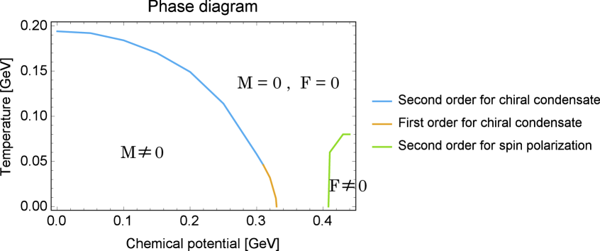
Figure 8: The phase diagram in this model is depicted. The horizontal and vertical axes represent the quark chemical potential and the temperature, respectively.

6 Summary and concluding remarks

In this paper, it has been shown that the spin polarized phase appears in the region with the large quark chemical potential and low temperature by using the NJL model with tensor-type four-point interaction between quarks. We have considered the chiral condensate and spin polarized condensate simultaneously. For rather low density, the chiral condensate exists and spin polarized condensate does not exist. As the quark chemical potential is increased, the chiral condensate disappears and further, the spin polarized condensate arises. Thus, the spin polarized phase may exist in the high density and low temperature region in QCD phase diagram. However, it may be concluded that the two phases do not coexist in this model under the parameter set adopted here.

It should be also indicated that the color superconducting phase may be realized in the region with high density and low temperature. However, at zero temperature, the spin polarized phase may be realized instead of the two-flavor color superconducting phase in the case with only two flavors [9]. It is interesting that the spin polarized phase survives or not at finite temperature instead of the color superconducting phase. It is one of future important problems to investigate. Furthermore, in this paper we do not consider the electromagnetic field at all. It is also important to study the electromagnetic properties in the spin polarized phase, for example, the spontaneous magnetization in compact stars. Especially, the charge neutrality and $\beta$-equilibrium play an essential role to discuss the physics of neutron stars and/or magnetars. It is also one of interesting future problems.

Appendix A Derivation of the thermodynamic potential at zero temperature from that at finite temperature

In this appendix we derive the thermodynamic potential at zero temperature from that at finite temperature. The thermodynamic potential at finite temperature is as follows:

$$\varOmega(M,F,\mu,T) =-\sum_{\eta,\tau,\alpha}\int_{\vec{p}^{2}\leq\varLambda^{2}}\frac{d^{3}p}{(2\pi)^{3}}\Biggl{\{}E^{(\eta)}_{\vec{p}}+T\log\left(1+\exp\left(-\frac{E^{(\eta)}_{\vec{p}}-\mu}{T}\right)\right)$$

$$\qquad\qquad\qquad\qquad\qquad\qquad\ \ +T\log\left(1+\exp\left(-\frac{E^{(\eta)}_{\vec{p}}+\mu}{T}\right)\right)\Biggl{\}}$$

$$+\frac{F^{2}}{2G_{\text{T}}}+\frac{M^{2}}{4G_{\text{S}}}.$$ (1.1)

If we assume $T\ll 1$, we can carry out the Taylor expansion for the logarithmic function in the following way:

$$T\log\left(1+\exp\left(-\frac{E^{(\eta)}_{\vec{p}}-\mu}{T}\right)\right)\rightarrow\begin{cases}-(E^{(\eta)}_{\vec{p}}-\mu)+T\exp\left(\frac{E^{(\eta)}_{\vec{p}}-\mu}{T}\right)&\text{for}\ E^{(\eta)}_{\vec{p}}\leq\mu\\ T\exp\left(-\frac{E^{(\eta)}_{\vec{p}}-\mu}{T}\right)&\text{for}\ E^{(\eta)}_{\vec{p}}>\mu,\end{cases}$$

$$T\log\left(1+\exp\left(-\frac{E^{(\eta)}_{\vec{p}}+\mu}{T}\right)\right)\rightarrow T\exp\left(-\frac{E^{(\eta)}_{\vec{p}}+\mu}{T}\right).\qquad\qquad\qquad\qquad\qquad\ \$$ (1.2)

Furthermore, in the region where $T\rightarrow 0$ we can reduce the above expressions into

$$T\log\left(1+\exp\left(-\frac{E^{(\eta)}_{\vec{p}}-\mu}{T}\right)\right)\rightarrow-(E^{(\eta)}_{\vec{p}}-\mu)\,\theta(\mu-E^{(\eta)}_{\vec{p}}),$$

$$T\log\left(1+\exp\left(-\frac{E^{(\eta)}_{\vec{p}}+\mu}{T}\right)\right)\rightarrow 0,\qquad\qquad\qquad\qquad\qquad$$ (1.3)

where $\theta(x)$ is the step function. Using these results, we could rewrite $\varOmega(M,F,\mu,T)$ into

$$\varOmega(M,F,\mu,T)\rightarrow -\sum_{\eta,\tau,\alpha}\int_{\vec{p}^{2}\leq\varLambda^{2}}\frac{d^{3}p}{(2\pi)^{3}}\left\{E^{(\eta)}_{\vec{p}}-(E^{(\eta)}_{\vec{p}}-\mu)\,\theta(\mu-E^{(\eta)}_{\vec{p}})\right\}$$

$$\ \ +\frac{F^{2}}{2G_{\text{T}}}+\frac{M^{2}}{4G_{\text{S}}}.$$ (1.4)

This expression is just one for the thermodynamic potential at zero temperature.

Appendix B Derivation for the effective potential with functional method

Let us start with the following Lagrangian density in order to derive the effective potential by using the functional method:

$$\mathcal{L} =\bar{\psi}(i\gamma^{\mu}\partial_{\mu}-m_{0})\psi+G_{S}(\bar{\psi}\psi)^{2}-\frac{G_{T}}{2}(\bar{\psi}\gamma^{1}\gamma^{2}\tau_{3}\psi)(\bar{\psi}\gamma_{1}\gamma_{2}\tau_{3}\psi)$$

$$=\bar{\psi}(i\gamma^{\mu}\partial_{\mu}-m_{0})\psi+G_{S}(\bar{\psi}\psi)^{2}+\frac{G_{T}}{2}(\bar{\psi}\varSigma_{3}\psi)^{2},$$ (2.1)

where we define $\varSigma_{3}\equiv-i\gamma^{1}\gamma^{2}$. In order to perform functional integral, let us introduce two auxiliary fields, $M^{\prime}$ and $F$, and use a relation of unit:

$$1=\int\mathcal{D}M^{\prime}\mathcal{D}F \exp\left[-i\int d^{4}x\left\{M^{\prime}+G_{S}(\bar{\psi}\psi)\right\}G^{-1}_{S}\left\{M^{\prime}+G_{S}(\bar{\psi}\psi)\right\}\right]$$

$$\times\exp\left[-\frac{i}{2}\int d^{4}x\left\{F+G_{T}(\bar{\psi}\varSigma_{3}\psi)\right\}G^{-1}_{T}\left\{F+G_{T}(\bar{\psi}\varSigma_{3}\psi)\right\}\right].$$ (2.2)

The generating functional $Z$ for the Lagrangian density (B1) is given as follows:

$$Z\propto\int\mathcal{D}\bar{\psi}\mathcal{D}\psi\exp\left[i\int d^{4}x\left\{\bar{\psi}(i\gamma^{\mu}\partial_{\mu}-m_{0})\psi+G_{S}(\bar{\psi}\psi)^{2}+\frac{G_{T}}{2}(\bar{\psi}\varSigma_{3}\psi)^{2}\right\}\right].$$ (2.3)

Inserting the relation of unit, (B2), into $Z$ and setting $M^{\prime}=M/2$, we obtain

$$Z\propto\int\mathcal{D}\bar{\psi}\mathcal{D}\psi\mathcal{D}M\mathcal{D}F\exp\left[i\int d^{4}x\left\{\bar{\psi}(i\gamma^{\mu}\partial_{\mu}-M_{q}-F\varSigma_{3})\psi-\frac{M^{2}}{4G_{S}}-\frac{F^{2}}{2G_{T}}\right\}\right],$$ (2.4)

where we define $M_{q}\equiv m_{0}+M$. Thus, we can integrate out with respect to $\psi$ and $\bar{\psi}$ easily. After some calculations, we get

$$Z \propto\int\mathcal{D}M\mathcal{D}F\;\text{Det}(i\gamma^{\mu}\partial_{\mu}-M_{q}-F\varSigma_{3})\exp\left[-i\int d^{4}x\left(\frac{M^{2}}{4G_{S}}+\frac{F^{2}}{2G_{T}}\right)\right]$$

$$=\int\mathcal{D}M\mathcal{D}F\exp\left[\text{Tr}\log\det(i\gamma^{\mu}\partial_{\mu}-M_{q}-F\varSigma_{3})-i\int d^{4}x\left(\frac{M^{2}}{4G_{S}}+\frac{F^{2}}{2G_{T}}\right)\right],$$ (2.5)

where in the second line the determinant, $\det$, operates on gamma matrices. In order to compute the trace, Tr, we change to momentum space.

$$Z\propto\int\mathcal{D}M\mathcal{D}F \exp\bigg{[}iN_{C}N_{F}\int d^{4}x\frac{d^{4}p}{i(2\pi)^{4}}\log\det(\not p-M_{q}-F\varSigma_{3})\bigg{]}$$

$$\times\exp\bigg{[}-i\int d^{4}x\left(\frac{M^{2}}{4G_{S}}+\frac{F^{2}}{2G_{T}}\right)\bigg{]},$$ (2.6)

where $N_{C}$ and $N_{F}$ mean the number of color and flavor, respectively. Our next step is to calculate the determinant. We can do it as follows:

$$\det(\not p-M_{q}-F\varSigma_{3})$$

$$=\det\gamma^{0}(\not p-M_{q}-F\varSigma_{3})$$

$$=\det\left[p^{0}-\gamma^{0}(\vec{\gamma}\cdot\vec{p}+M_{q}+F\varSigma_{3})\right]$$

$$=\det\left[p^{0}-\begin{pmatrix}E^{(+)}_{\vec{p}}&&&\\ &E^{(-)}_{\vec{p}}&&\\ &&-E^{(+)}_{\vec{p}}&\\ &&&-E^{(-)}_{\vec{p}}\end{pmatrix}\right]$$

$$=(p^{0}-E^{(+)}_{\vec{p}})(p^{0}-E^{(-)}_{\vec{p}})(p^{0}+E^{(+)}_{\vec{p}})(p^{0}+E^{(-)}_{\vec{p}})\ .$$ (2.7)

Substituting the above result into $Z$ in (B6), we obtain

$$Z\propto\int \mathcal{D}M\mathcal{D}F$$

$$\times\exp\left[iN_{C}N_{F}\int d^{4}x\frac{d^{4}p}{i(2\pi)^{4}}\log(p^{0}-E^{(+)}_{\vec{p}})(p^{0}-E^{(-)}_{\vec{p}})(p^{0}+E^{(+)}_{\vec{p}})(p^{0}+E^{(-)}_{\vec{p}})\right]$$

$$\times\exp\left[-i\int d^{4}x\left(\frac{M^{2}}{4G_{S}}+\frac{F^{2}}{2G_{T}}\right)\right].$$ (2.8)

For a little while, we consider the only contents of exponential in the second line in (B8):

$$\int\frac{d^{4}p}{i(2\pi)^{4}}\log(p^{0}-E^{(+)}_{\vec{p}})(p^{0}-E^{(-)}_{\vec{p}})(p^{0}+E^{(+)}_{\vec{p}})(p^{0}+E^{(-)}_{\vec{p}}).$$ (2.9)

Let us differentiate and integrate the above expression with respect to $E^{(+)}_{\vec{p}}$ and $E^{(-)}_{\vec{p}}$. As a result, (B9) can be recast into

$$\int\frac{d^{4}p}{i(2\pi)^{4}} \int dE^{(+)}_{\vec{p}}\left(\frac{1}{p^{0}+E^{(+)}_{\vec{p}}}-\frac{1}{p^{0}-E^{(+)}_{\vec{p}}}\right)$$

$$+\int\frac{d^{4}p}{i(2\pi)^{4}}\int dE^{(-)}_{\vec{p}}\left(\frac{1}{p^{0}+E^{(-)}_{\vec{p}}}-\frac{1}{p^{0}-E^{(-)}_{\vec{p}}}\right).$$ (2.10)

We would like to discuss a system at finite temperature and density. So let us change the integration to the summation by using the Matsubara method as follows:

$$\int\frac{d^{4}p}{i(2\pi)^{4}}f(p^{0},\vec{p})\rightarrow T\sum_{n=-\infty}^{\infty}\int\frac{d^{3}p}{(2\pi)^{3}}f(i\omega_{n}+\mu,\vec{p}),$$ (2.11)

where $\omega_{n}$ is the Matsubara frequency and $\mu$ is chemical potential. Using a formula

$$\lim_{\epsilon\rightarrow+0}T\sum_{n}\frac{e^{i\omega_{n}\epsilon}}{i\omega_{n}-x}=\lim_{\epsilon\rightarrow+0}\frac{e^{i\omega_{n}\epsilon}}{e^{x/T}+1}=\frac{1}{e^{x/T}+1},$$ (2.12)

we can calculate the summation following the standard technique. As a result, we obtain

$$\sum_{\eta=\pm}\int\frac{d^{3}p}{(2\pi)^{3}}\left[E^{(\eta)}_{\vec{p}}+\mu+T\log\left\{1+\exp\left(-\frac{E^{(\eta)}_{\vec{p}}+\mu}{T}\right)\right\}\right.$$

$$\qquad\qquad\qquad\qquad\qquad\left.+T\log\left\{1+\exp\left(-\frac{E^{(\eta)}_{\vec{p}}-\mu}{T}\right)\right\}\right].$$ (2.13)

Substituting the above result into $Z$, $Z$ can be expressed as

$$Z\propto\int\mathcal{D}M\mathcal{D}F\exp i \bigg{[}N_{C}N_{F}\int d^{4}x\frac{d^{3}p}{(2\pi)^{3}}\sum_{\eta}\bigg{(}E^{(\eta)}_{\vec{p}}+T\log\bigg{\{}1+\exp\bigg{(}-\frac{E^{(\eta)}_{\vec{p}}+\mu}{T}\bigg{)}\bigg{\}}$$

$$+T\log\bigg{\{}1+\exp\bigg{(}-\frac{E^{(\eta)}_{\vec{p}}-\mu}{T}\bigg{)}\bigg{\}}\bigg{)}-\int d^{4}x\bigg{(}\frac{M^{2}}{4G_{S}}+\frac{F^{2}}{2G_{T}}\bigg{)}\bigg{]},$$ (2.14)

where we neglect a constant term. In general, the effective action $\varGamma$ and effective potential $V$ are defined as follows:

$$Z=\exp\left(i\varGamma[M,F,T,\mu]\right),\ \qquad V[M,F,T,\mu]=-\frac{\varGamma[M,F,T,\mu]}{\int d^{4}x}.$$ (2.15)

Thus, finally, we obtain the effective potential $V$ as

$$V[M,F,T,\mu]= -N_{C}N_{F}\int\frac{d^{3}p}{(2\pi)^{3}}\sum_{\eta}\bigg{[}E^{(\eta)}_{\vec{p}}+T\log\bigg{\{}1+\exp\bigg{(}-\frac{E^{(\eta)}_{\vec{p}}+\mu}{T}\bigg{)}\bigg{\}}$$

$$+T\log\bigg{\{}1+\exp\bigg{(}-\frac{E^{(\eta)}_{\vec{p}}-\mu}{T}\bigg{)}\bigg{\}}\bigg{]}+\frac{M^{2}}{4G_{S}}+\frac{F^{2}}{2G_{T}}.$$ (2.16)

This is identical with the thermodynamic potential (4).

Appendix C The domain of integral with respect to the three-momentum in the thermodynamic potential at zero temperature

In 3, we gave the expression of the thermodynamic potential. In this appendix, we give a domain of integral with respect to three-momentum carefully. We assume $M\geq 0$, $F\geq 0$ and $\varLambda>\mu$ without loss of generality and introduce polar coordinates ($p_{T},\theta$):

$$p_{1}=p_{T}\cos\theta,\,\qquad p_{2}=p_{T}\sin\theta.$$

Moreover, we define $q\equiv\sqrt{p_{T}^{2}+M_{\text{q}}^{2}}$ in order to integrate over momenta. After integrating over $\theta$ in Eqs.(3.4) - (3.6), we obtain the thermodynamic potential $\varPhi=\sum_{i=1}^{4}\varPhi_{i}$ as follows:

$$\varPhi_{1}(M,F,\mu)= \frac{3}{2\pi^{2}}\int_{\varGamma_{1}}dqdp_{3}\,q\left(\sqrt{p_{3}^{2}+(q+F)^{2}}-\mu\right),$$

$$\varGamma_{1}=\left\{p_{3}^{2}+(q+F)^{2}\leq\mu^{2},p_{3}^{2}+q^{2}\leq\varLambda^{2}+M^{2}_{\text{q}},q\geq M_{\text{q}}\right\}$$

$$\varPhi_{2}(M,F,\mu)= \frac{3}{2\pi^{2}}\int_{\varGamma_{2}}dqdp_{3}\,q\left(\sqrt{p_{3}^{2}+(q-F)^{2}}-\mu\right),$$

$$\varGamma_{2}=\left\{p_{3}^{2}+(q-F)^{2}\leq\mu^{2},p_{3}^{2}+q^{2}\leq\varLambda^{2}+M^{2}_{\text{q}},q\geq M_{\text{q}}\right\}$$

$$\varPhi_{3}(M,F,\mu)= -\frac{3}{2\pi^{2}}\sum_{\eta}\int_{\varGamma_{3}}dqdp_{3}\,q\sqrt{p_{3}^{2}+(q+\eta F)^{2}},\qquad\qquad\qquad$$

$$\varGamma_{3}=\left\{p_{3}^{2}+q^{2}\leq\varLambda^{2}+M^{2}_{\text{q}},q\geq M_{\text{q}}\right\}$$

$$\varPhi_{4}(M,F,\mu)=\frac{M^{2}}{4G_{\text{S}}}+\frac{F^{2}}{2G_{\text{T}}}.\qquad\qquad\qquad\qquad\qquad\qquad\qquad\qquad\quad$$

Further, let us integrate the thermodynamic potential over $p_{3}$ analytically. To do this we must discuss the domain of the integral carefully. First we consider $\varPhi_{1}$ and $\varGamma_{1}$. If the first condition in $\varGamma_{1}$ is satisfied, the second condition in it will be satisfied automatically. So we could reduce $\varGamma_{1}$ to

$$\varGamma_{1}=\left\{p_{3}^{2}+(q+F)^{2}\leq\mu^{2},q\geq M_{\text{q}}\right\}.$$

Furthermore, we could change the above condition to as follows:

$$\varGamma_{1}=\left\{-\sqrt{\mu^{2}-(q+F)^{2}}\leq p_{3}\leq\sqrt{\mu^{2}-(q+F)^{2}},\;q\geq M_{\text{q}}\right\}.$$

Since the contents in a square root must be positive, the final form is

$$\varGamma_{1}=\left\{-\sqrt{\mu^{2}-(q+F)^{2}}\leq p_{3}\leq\sqrt{\mu^{2}-(q+F)^{2}},\;M_{\text{q}}\leq q\leq\mu-F\right\}.$$

However, we need the condition: $M_{\text{q}}\leq\mu-F$ in order to integrate over $q$. If $M_{\text{q}}>\mu-F$, we can not perform integral. Using an integration formula:

$$\int dx\,\sqrt{x^{2}+a^{2}}=\frac{1}{2}\left\{x\sqrt{x^{2}+a^{2}}+a^{2}\log\left(x+\sqrt{x^{2}+a^{2}}\right)\right\},$$

we were able to perform integral over $p_{3}$ easily. The final results are the following:

$${\rm If}\ M_{\text{q}}>\mu-F,$$

$$\quad\varPhi_{1}(M,F,\mu)=0.$$ (3.1a)

$${\rm If}\ M_{\text{q}}\leq\mu-F,$$

$$\quad\varPhi_{1}(M,F,\mu)=\frac{3}{2\pi^{2}}\int_{M_{\text{q}}}^{\mu-F}dq\,q\biggl{\{}-\mu\sqrt{\mu^{2}-(q+F)^{2}}$$

$$\qquad\qquad\qquad\qquad\qquad\qquad\quad+(q+F)^{2}\log\left(\frac{\sqrt{\mu^{2}-(q+F)^{2}}+\mu}{q+F}\right)\biggl{\}}.\ \$$ (3.1b)

Next, we consider $\varPhi_{2}$ and $\varGamma_{2}$. This case is more complicated than the previous case. There are five cases for conditions to perform integral as follows:

If $F-\mu\leq M_{\text{q}}\leq F+\mu\leq\sqrt{\varLambda^{2}+M^{2}_{\text{q}}}$,

$$\varPhi_{2}(M,F,\mu)=\frac{3}{2\pi^{2}}\int_{M_{\text{q}}}^{F+\mu}dq\int_{-\sqrt{\mu^{2}-(q-F)^{2}}}^{\sqrt{\mu^{2}-(q-F)^{2}}}dp_{3}\,q\left(\sqrt{p_{3}^{2}+(q-F)^{2}}-\mu\right).$$

If $M_{\text{q}}\leq F-\mu\leq F+\mu\leq\sqrt{\varLambda^{2}+M^{2}_{\text{q}}}$,

$$\varPhi_{2}(M,F,\mu)=\frac{3}{2\pi^{2}}\int_{F-\mu}^{F+\mu}dq\int_{-\sqrt{\mu^{2}-(q-F)^{2}}}^{\sqrt{\mu^{2}-(q-F)^{2}}}dp_{3}\,q\left(\sqrt{p_{3}^{2}+(q-F)^{2}}-\mu\right).$$

If $M_{\text{q}}\leq F-\mu\leq b\leq\sqrt{\varLambda^{2}+M^{2}_{\text{q}}}\leq F+\mu$,

$$\varPhi_{2}(M,F,\mu) =\frac{3}{2\pi^{2}}\left(\int^{b}_{F-\mu}\int_{-\sqrt{\mu^{2}-(q-F)^{2}}}^{\sqrt{\mu^{2}-(q-F)^{2}}}+\int_{b}^{\sqrt{\varLambda^{2}+M^{2}_{\text{q}}}}\int_{-\sqrt{\varLambda^{2}+M^{2}_{\text{q}}-q^{2}}}^{\sqrt{\varLambda^{2}+M^{2}_{\text{q}}-q^{2}}}\right)$$

$$\times q\left(\sqrt{p_{3}^{2}+(q-F)^{2}}-\mu\right)dp_{3}\,dq.$$

If $F-\mu\leq M_{\text{q}}\leq b\leq\sqrt{\varLambda^{2}+M^{2}_{\text{q}}}\leq F+\mu$,

$$\varPhi_{2}(M,F,\mu) =\frac{3}{2\pi^{2}}\left(\int^{b}_{M_{\text{q}}}\int_{-\sqrt{\mu^{2}-(q-F)^{2}}}^{\sqrt{\mu^{2}-(q-F)^{2}}}+\int_{b}^{\sqrt{\varLambda^{2}+M^{2}_{\text{q}}}}\int_{-\sqrt{\varLambda^{2}+M^{2}_{\text{q}}-q^{2}}}^{\sqrt{\varLambda^{2}+M^{2}_{\text{q}}-q^{2}}}\right)$$

$$\times q\left(\sqrt{p_{3}^{2}+(q-F)^{2}}-\mu\right)dp_{3}\,dq.$$

If $F-\mu\leq b\leq M_{\text{q}}\leq\sqrt{\varLambda^{2}+M_{\text{q}}}\leq F+\mu$,

$$\varPhi_{2}(M,F,\mu)=\frac{3}{2\pi^{2}}\int_{M_{\text{q}}}^{\sqrt{\varLambda^{2}+M^{2}_{\text{q}}}}dq\int_{-\sqrt{\varLambda^{2}+M^{2}_{\text{q}}-q^{2}}}^{\sqrt{\varLambda^{2}+M^{2}_{\text{q}}-q^{2}}}dp_{3}\,q\left(\sqrt{p_{3}^{2}+(q-F)^{2}}-\mu\right).$$

Here, $b$ is the solution for $q$ of the simultaneous equation:

$$p_{3}^{2}+q^{2}=\varLambda^{2}+M^{2}_{\text{q}}\ ,\qquad p_{3}^{2}+(q-F)^{2}=\mu^{2}$$

We were able to perform integral over $p_{3}$, then define two functions for simplicity as follows:

$$\phi_{1}(q)\equiv\frac{3}{2\pi^{2}}q\left\{-\mu\sqrt{\mu^{2}-(F-q)^{2}}+(F-q)^{2}\log\left(\frac{\mu+\sqrt{\mu^{2}-(F-q)^{2}}}{|F-q|}\right)\right\},\ \$$

$$\phi_{2}(q) \equiv\frac{3}{2\pi^{2}}q\Biggl{\{}\sqrt{\varLambda^{2}+M^{2}_{\text{q}}-q^{2}}\left(-2\mu+\sqrt{F^{2}+\varLambda^{2}+M^{2}_{\text{q}}-2Fq}\right)$$

$$\qquad\qquad+(F-q)^{2}\log\left(\frac{\sqrt{F^{2}+\varLambda^{2}+M^{2}_{\text{q}}-2Fq}+\sqrt{\varLambda^{2}+M^{2}_{\text{q}}-q^{2}}}{|F-q|}\right)\Biggr{\}}.$$

Using the above expressions, the final results are summarized as follows:

$${\rm If}\ F-\mu\leq M_{\text{q}}\leq F+\mu\leq\sqrt{\varLambda^{2}+M^{2}_{\text{q}}},$$

$$\qquad\varPhi_{2}(M,F,\mu)=\int_{M_{\text{q}}}^{F+\mu}dq\,\phi_{1}(q).$$ (3.2a)

$${\rm If}\ M_{\text{q}}\leq F-\mu\leq F+\mu\leq\sqrt{\varLambda^{2}+M^{2}_{\text{q}}},$$

$$\qquad\varPhi_{2}(M,F,\mu)=\int_{F-\mu}^{F+\mu}dq\,\phi_{1}(q).$$ (3.2b)

$${\rm If}\ M_{\text{q}}\leq F-\mu\leq b\leq\sqrt{\varLambda^{2}+M^{2}_{\text{q}}}\leq F+\mu,$$

$$\qquad\varPhi_{2}(M,F,\mu)=\int^{b}_{F-\mu}dq\,\phi_{1}(q)+\int_{b}^{\sqrt{\varLambda^{2}+M^{2}_{\text{q}}}}dq\,\phi_{2}(q).$$ (3.2c)

$${\rm If}\ F-\mu\leq M_{\text{q}}\leq b\leq\sqrt{\varLambda^{2}+M^{2}_{\text{q}}}\leq F+\mu,$$

$$\qquad\varPhi_{2}(M,F,\mu)=\int^{b}_{M_{\text{q}}}dq\,\phi_{1}(q)+\int_{b}^{\sqrt{\varLambda^{2}+M^{2}_{\text{q}}}}dq\,\phi_{2}(q).$$ (3.2d)

$${\rm If}\ F-\mu\leq b\leq M_{\text{q}}\leq\sqrt{\varLambda^{2}+M_{\text{q}}}\leq F+\mu,$$

$$\qquad\varPhi_{2}(M,F,\mu)=\int_{M_{\text{q}}}^{\sqrt{\varLambda^{2}+M^{2}_{\text{q}}}}d\,q\phi_{2}(q).$$ (3.2e)

Finally, we discuss $\varPhi_{3}$ and $\varGamma_{3}$. We could derive the domain of integral easily in this case. The domain is re-expressed as

$$\varGamma_{3}=\left\{-\sqrt{\varLambda^{2}+M^{2}_{\text{q}}-q^{2}}\leq p_{3}\leq\sqrt{\varLambda^{2}+M^{2}_{\text{q}}-q^{2}},\ M_{\text{q}}\leq q\leq\sqrt{\varLambda^{2}+M^{2}_{\text{q}}}\right\}.$$

After integrating over $p_{3}$, we obtain the final result:

$$\varPhi_{3}(M,F,\mu) =-\frac{3}{2\pi^{2}}\sum_{\eta}\int_{M_{\text{q}}}^{\sqrt{\varLambda^{2}+M^{2}_{\text{q}}}}dq\,q\Biggl{\{}\sqrt{\varLambda^{2}+M^{2}_{\text{q}}-q^{2}}\sqrt{\varLambda^{2}+M^{2}_{\text{q}}+2\eta qF+F^{2}}$$

$$+(q+\eta F)^{2}\log\left(\frac{\sqrt{\varLambda^{2}+M^{2}_{\text{q}}-q^{2}}+\sqrt{\varLambda^{2}+M^{2}_{\text{q}}+2\eta qF+F^{2}}}{|q+\eta F|}\right)\Biggr{\}}.$$ (3.3)

Appendix D A possibility of origin of tensor-type interaction in NJL model

In the QCD Lagrangian, the interaction part is written as

$${\cal L}_{\rm int}=g{\bar{\psi}}(x)\gamma^{\mu}\psi(x)A_{\mu}(x)\ ,$$ (4.1)

where $\psi(x)$ and $A_{\mu}(x)\ (=A_{\mu}^{a}(x)T^{a})$ are quark and gluon fields, respectively, and $T^{a}$ represents the color $su(3)$-generators. Here, two-gluon exchange diagram is properly depicted in Fig.9. These diagrams are obtained from fourth-order perturbation of ${\cal L}_{\rm int}$:

$$\int d^{4}x{\cal L}_{\rm int}(x)\cdot\int d^{4}y{\cal L}_{\rm int}(y)\cdot\int d^{4}x{\cal L}_{\rm int}(x^{\prime})\cdot\int d^{4}x{\cal L}_{\rm int}(y^{\prime})$$ (4.2)

$$= g^{4}\int d^{4}xd^{4}yd^{4}x^{\prime}d^{4}y^{\prime}{\bar{\psi}}(x)\gamma^{\mu}\psi(x)A_{\mu}(x){\bar{\psi}}(y)\gamma^{\nu}\psi(y)A_{\nu}(y)$$

$$\qquad\qquad\qquad\qquad\times{\bar{\psi}}(x^{\prime})\gamma^{\rho}\psi(x^{\prime})A_{\rho}(x^{\prime}){\bar{\psi}}(y^{\prime})\gamma^{\sigma}\psi(y^{\prime})A_{\sigma}(y^{\prime})\ .\qquad$$

We here intend to describe the above expression as

$$\int d^{4}x{\cal L}_{\rm eff}\ ,$$ (4.3)

which should be expressed as the four-point interaction between quarks.

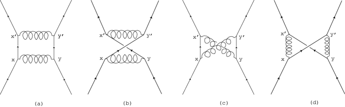
Figure 9: The Feynman diagrams of proper two-gluon exchange process.

As for the process in Fig.9 (a) and (b), these process may mainly be regarded as the repeated processes of one-gluon exchange process. Thus, we omit these process in proper contribution of two-gluon exchange process. Therefore, let us first consider the diagram in Fig.9 (c). Writing the spinor indices, $i,j,\cdots$, explicitly, we contract bilinear field making the Feynman propagator:

$$g^{4}\int d^{4}xd^{4}yd^{4}x^{\prime}d^{4}y^{\prime}{\bar{\psi}}_{i}(x)\gamma^{\mu}_{ij}{\psi}_{j}(x)A_{\mu}(x){\bar{\psi}}_{k}(y)\gamma^{\nu}_{kl}\psi_{l}(y)A_{\nu}(y)$$

$$\qquad\qquad\qquad\qquad\times{{\bar{\psi}}}_{m}(x^{\prime})\gamma^{\rho}_{mn}\psi_{n}(x^{\prime})A_{\rho}(x^{\prime}){\bar{\psi}}_{p}(y^{\prime})\gamma^{\sigma}_{pq}\psi_{q}(y^{\prime})A_{\sigma}(y^{\prime})$$

$$\longrightarrow g^{4}\int d^{4}xd^{4}yd^{4}x^{\prime}d^{4}y^{\prime}{\cal L}_{(c)}\ ,$$

$${\cal L}_{(c)}=-{\bar{\psi}}_{i}(x)\gamma^{\mu}_{ij}{\bar{\psi}}_{k}(y)\gamma^{\nu}_{kl}\gamma^{\rho}_{mn}\psi_{n}(x^{\prime})\gamma^{\sigma}_{pq}\psi_{q}(y^{\prime})$$

$$\qquad\qquad\qquad\qquad\times\langle\psi_{j}(x){\bar{\psi}}_{m}(x^{\prime})\rangle\langle A_{\mu}(x)A_{\sigma}(y^{\prime})\rangle\langle\psi_{l}(y){\bar{\psi}}_{p}(y^{\prime})\rangle\langle A_{\nu}(y)A_{\rho}(x^{\prime})\rangle.$$ (4.4)

Here, it should be noted that the property of Grassmann number for fermion field is used. Thus, a minus sign appears. Here, $\langle\psi_{i}(x){\bar{\psi}}_{j}(y)\rangle$ and $\langle A_{\mu}(x)A_{\nu}(y)\rangle\ (=T^{a}T^{b}\langle A_{\mu}^{a}(x)A_{\nu}^{b}(y)\rangle)$ represent the Feynman propagator for quark and gluon fields, respectively:

$$\langle\psi_{i}(x){\bar{\psi}}_{j}(y)\rangle=\int\frac{d^{4}p}{i(2\pi)^{4}}\frac{\gamma^{\mu}p_{\mu}+M_{q}}{M_{q}^{2}-p^{2}-i\epsilon}e^{-ip(x-y)}\ ,$$

$$\langle A_{\mu}^{a}(x)A_{\nu}^{b}(y)\rangle=\delta^{ab}\int\frac{d^{4}p}{i(2\pi)^{4}}\frac{1}{p^{2}+i\epsilon}\left[g_{\mu\nu}-(1-\alpha)\frac{p_{\mu}p_{\nu}}{p^{2}}\right]e^{-ip(x-y)}\ ,$$ (4.5)

where $a$ and $b$ are color indices, $M_{q}$ is the quark mass and $\alpha$ is a gauge parameter. Of course, the NJL model Lagrangian cannot be derived from QCD. Therefore, we have to give up the exact calculation. Thus, we assume the form of propagators so as to reproduce the four-point contact interaction between quarks. As for the quark propagator, the quark mass in the propagator is set to very large value or infinity artificially:

$$\langle\psi_{i}(x){\bar{\psi}}_{j}(y)\rangle\sim\int\frac{d^{4}p}{i(2\pi)^{4}}\frac{1_{ij}}{M_{q}}e^{-ip(x-y)}=\frac{1}{iM_{q}}\delta_{ij}\delta^{4}(x-y)\ .$$ (4.6)

As for the gluon propagator, artificially “gluon mass” $M_{g}$ is introduced and is taken as a very large value or infinity.

$$\langle A_{\mu}^{a}(x)A_{\nu}^{b}(y)\rangle = \delta^{ab}\int\frac{d^{4}p}{i(2\pi)^{4}}\frac{1}{p^{2}+i\epsilon}\left[g_{\mu\nu}-(1-\alpha)\frac{p_{\mu}p_{\nu}}{p^{2}}\right]e^{-ip(x-y)}$$ (4.7)

$$\rightarrow \delta^{ab}\int\frac{d^{4}p}{i(2\pi)^{4}}\frac{1}{p^{2}-M_{g}^{2}+i\epsilon}\left[g_{\mu\nu}-(1-\alpha)\frac{p_{\mu}p_{\nu}}{p^{2}}\right]e^{-ip(x-y)}$$

$$\sim \delta^{ab}\int\frac{d^{4}p}{i(2\pi)^{4}}\frac{g_{\mu\nu}}{-M_{g}^{2}}e^{-ip(x-y)}=-\frac{1}{iM_{g}^{2}}\delta^{ab}g_{\mu\nu}\delta^{4}(x-y).$$

Hereafter, we denote $M_{q}^{2}M_{g}^{4}\equiv M_{\rm eff}^{6}$, in which $M_{\rm eff}$ has mass-dimension. Inserting the above “approximate” propagators into Eq.(D), then, Eq.(D) is rewritten as

$${\cal L}_{(c)}=\frac{C_{2}^{2}}{M_{\rm eff}^{6}}{\bar{\psi}}_{i}(x)\gamma^{\mu}_{ij}\gamma^{\rho}_{jn}\psi_{n}(x){\bar{\psi}}_{k}(x)\gamma_{\rho,kl}\gamma_{\mu,lq}\psi_{q}(x)$$

$$\qquad\qquad\qquad\qquad\qquad\times\delta^{4}(x-x^{\prime})\delta^{4}(x^{\prime}-y)\delta^{4}(x-y^{\prime})\delta^{4}(y^{\prime}-y),$$ (4.8)

where $C_{2}=\sum_{a}T^{a}T^{a}$. Here, we use again the property of Grassmann number. Thus, we obtain

$$g^{4}\int d^{4}xd^{4}yd^{4}x^{\prime}d^{4}y^{\prime}{\cal L}_{(c)} = \frac{g^{4}\delta^{4}(0)}{M_{\rm eff}^{6}}\cdot C_{2}^{2}\int d^{4}x\ {\bar{\psi}}(x)\gamma^{\mu}\gamma^{\rho}\psi(x)\cdot{\bar{\psi}}(x)\gamma_{\rho}\gamma_{\mu}\psi(x)$$ (4.9)

$$= -g_{T}\int d^{4}x{\bar{\psi}}(x)\gamma^{\mu}\gamma^{\nu}\psi(x)\cdot{\bar{\psi}}(x)\gamma_{\mu}\gamma_{\nu}\psi(x)$$

$$+8g_{T}\int d^{4}x{\bar{\psi}}(x)\psi(x)\cdot{\bar{\psi}}(x)\psi(x)\ ,$$

where we define $g_{T}=g^{4}\delta^{4}(0)C_{2}^{2}/M_{\rm eff}^{6}\ (>0)$ and use $\gamma^{\mu}\gamma^{\nu}+\gamma^{\nu}\gamma^{\mu}=2g^{\mu\nu}$ and $\gamma^{\mu}\gamma_{\mu}=4$. Here, $\delta^{4}(0)=\int d^{4}k/(2\pi)^{4}\cdot\left.e^{ik(x-y)}\right|_{x=y}$ which is regarded as a very large value or infinity in order to $g_{T}$ has a finite value. Then, $g_{T}$ has a dimension of (mass)^-2.

Next, let us consider Fig.9 (d). As is similar to the case Fig.9 (c), we obtain

$$g^{4}\int d^{4}xd^{4}yd^{4}x^{\prime}d^{4}y^{\prime}{\bar{\psi}}_{i}(x)\gamma^{\mu}_{ij}{\psi}_{j}(x)A_{\mu}(x){\bar{\psi}}_{k}(y)\gamma^{\nu}_{kl}\psi_{l}(y)A_{\nu}(y)$$

$$\qquad\qquad\qquad\qquad\times{{\bar{\psi}}}_{m}(x^{\prime})\gamma^{\rho}_{mn}\psi_{n}(x^{\prime})A_{\rho}(x^{\prime}){\bar{\psi}}_{p}(y^{\prime})\gamma^{\sigma}_{pq}\psi_{q}(y^{\prime})A_{\sigma}(y^{\prime})$$

$$\longrightarrow g^{4}\int d^{4}xd^{4}yd^{4}x^{\prime}d^{4}y^{\prime}{\cal L}_{(d)\ ,}$$

$${\cal L}_{(d)}={\bar{\psi}}_{i}(x)\gamma^{\mu}_{ij}{\bar{\psi}}_{k}(y)\gamma^{\nu}_{kl}\gamma^{\rho}_{mn}\psi_{n}(x^{\prime})\gamma^{\sigma}_{pq}\psi_{q}(y^{\prime})$$

$$\qquad\qquad\qquad\qquad\times\langle\psi_{l}(y){\bar{\psi}}_{m}(x^{\prime})\rangle\langle A_{\mu}(x)A_{\rho}(x^{\prime})\rangle\langle\psi_{j}(x){\bar{\psi}}_{p}(y^{\prime})\rangle\langle A_{\nu}(y)A_{\sigma}(y^{\prime})\rangle.\quad$$ (4.10)

In order to obtain the four-point contact interaction for NJL type, we “approximate” the propagators in (4.6) and (4.7). Then,

$${\cal L}_{(d)}=\frac{C_{2}^{2}}{M_{\rm eff}^{6}}{\bar{\psi}}_{i}(x)\gamma^{\mu}_{ij}\gamma^{\sigma}_{jq}\psi_{q}(x){\bar{\psi}}_{k}(x)\gamma_{\sigma,kl}\gamma_{\mu,ln}\psi_{n}(x)$$

$$\qquad\qquad\qquad\qquad\times\delta^{4}(x-x^{\prime})\delta^{4}(x^{\prime}-y)\delta^{4}(x-y^{\prime})\delta^{4}(y^{\prime}-y)$$

is obtained. Therefore,

$$g^{4}\int d^{4}xd^{4}yd^{4}x^{\prime}d^{4}y^{\prime}{\cal L}_{(d)} = \frac{g^{4}\delta^{4}(0)}{M_{\rm eff}^{6}}\cdot C_{2}^{2}\int d^{4}x\ {\bar{\psi}}(x)\gamma^{\mu}\gamma^{\nu}\psi(x)\cdot{\bar{\psi}}(x)\gamma_{\nu}\gamma_{\mu}\psi(x)$$ (4.12)

$$= -g_{T}\int d^{4}x{\bar{\psi}}(x)\gamma^{\mu}\gamma^{\nu}\psi(x)\cdot{\bar{\psi}}(x)\gamma_{\mu}\gamma_{\nu}\psi(x)$$

$$+8g_{T}\int d^{4}x{\bar{\psi}}(x)\psi(x)\cdot{\bar{\psi}}(x)\psi(x)\ ,$$

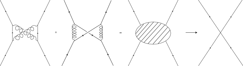
Figure 10: The Feynman diagrams of two-gluon exchange process.

Finally, we obtain the effective Lagrangian density originated from the properly two-gluon exchange contribution between quarks, as is illustrated in Fig.10, as follows:

$$\int d^{4}x{\cal L}_{\rm eff} = g^{4}\int d^{4}xd^{4}yd^{4}x^{\prime}d^{4}y^{\prime}({\cal L}_{(c)}+{\cal L}_{(d)})$$

$$= \int d^{4}x\left(-\frac{G_{T}}{4}{\bar{\psi}}(x)\gamma^{\mu}\gamma^{\nu}\psi(x)\cdot{\bar{\psi}}(x)\gamma_{\mu}\gamma_{\nu}\psi(x)+2G_{T}{\bar{\psi}}(x)\psi(x)\cdot{\bar{\psi}}(x)\psi(x)\right)\ ,$$

where we define $G_{T}\equiv 8g_{T}$ where $G_{T}>0$. We take $G_{T}=11$ GeV^-2 in this paper. The first term corresponds to our tensor-type four-point interaction. Introducing the degree of freedom of the flavor, the tensor-part is written as

$${\cal L}_{T}=-\frac{G_{T}}{4}({\bar{\psi}}\gamma^{\mu}\gamma^{\nu}{\overrightarrow{\tau}}\psi)({\bar{\psi}}\gamma_{\mu}\gamma_{\nu}{\overrightarrow{\tau}}\psi)\ .$$ (4.14)

which is identical with the first term in Eq.(2.4). Of coure, the above treatment is nothing but a crude approximate treatment. Thus, we have to add another term so as to retain the chiral symmetry that the QCD has. The second term in Eq. (D) represents the scalar-scalar interaction appearing in the original NJL model Lagrangian. However, the one-gluon exchange contribution may be wash out this contribution from two-gluon exchange.

References

• [1] See, for example, K. Fukushima and T. Hatsuda, Rep. Prog. Phys. 74, 014001 (2011).
• [2] M. G. Alford, A. Schmitt, K. Rajagopal and T. Schafer, Rev. Mod. Phys. 80, 1455 (2008) and references cited therein.
• [3] M. Alford, K. Rajagopal and F. Wilczek, Nucl. Phys. B 537, 443 (1999).
• [4] K. Iida and G. Baym, Phys. Rev. D 63, 074018 (2001).
• [5] L. McLerran and R. D. Pisarski, Nucl. Phys. A 796, 83 (2007).
• [6] E. Nakano and T. Tatsumi, Phys. Rev. D 71, 114006 (2005).
• [7] D. Nickel, Phys. Rev. Lett. 103, 072301 (2009).
• [8] M. Buballa and S. Carignano, Prog. Part. Nucl. Phys. 81, 39 (2015), and references cited therein.
• [9] Y. Tsue, J. da Providência, C. Providêncis, M. Yamamura and H. Bhor, Prog. Theor. Exp. Phys. 2013, 103D01 (2013).
• [10] Y. Tsue, J. da Providência, C. Providêncis, M. Yamamura and H. Bhor, Prog. Theor. Exp. Phys. 2015, 013D02 (2015).
• [11] Y. Tsue, J. da Providência, C. Providêncis, M. Yamamura and H. Bhor, Prog. Theor. Exp. Phys. 2015, 103D01 (2015).
• [12] R. C. Duncan and C. Thompson, Astrophys. J. 392, L9 (1992).
• [13] C. Thompson and R. C. Duncan, Astrophys. J. 408, 194 (1993).
• [14] C. Thompson and R. C. Duncan, Astrophys. J. 473, 322 (1996).
• [15] Y. Tsue, J. da Providência, C. Providêncis and M. Yamamura, Prog. Theor. Phys. 128, 507 (2012).
• [16] Y. Nambu and G. Jona-Lasinio, Phys. Rev. 122, 345 (1961), Phys. Rev 124, 246 (1961).
• [17] T. Hatsuda and T. Kunihiro, Phys. Rep. 247, 221 (1994).
• [18] M. Buballa, Phys. Rep. 407, 205 (2005).
• [19] H. Bohr, P. K. Panda, C. Providência and J. da Providência, Int. J. Mod. Phys. E 22, 1350019 (2013).
• [20] E. Nakano, T. Maruyama and T. Tatsumi, Phys. Rev. D 68, 105001 (2003).
• [21] T. Tatsumi, T. Maruyama and E. Nakano, Prog. Theor. Phys. Suppl. No. 153, 190 (2004).
• [22] M. Jaminon, E. Ruiz Arriola, Phys. Lett. B 443, 33 (1998).
• [23] M. Chizhov, JETP Lett. 80, 73 (2004).
• [24] E. J. Ferrer, V. de la Incera, I. Portillo and M. Quiroz, Phys. Rev. D 89, 085034 (2014).