Post-quench dynamics and pre-thermalization in a resonant Bose gas

Abstract

We explore the dynamics of a resonant Bose gas following its quench to a strongly interacting regime near a Feshbach resonance. For such deep quenches, we utilize a self-consistent dynamic field approximation and find that after an initial regime of many-body Rabi-like oscillations between the condensate and finite-momentum quasiparticle pairs, at long times, the gas reaches a pre-thermalized nonequilibrium steady state. We explore the resulting state through its broad stationary momentum distribution function, that exhibits a power-law high momentum tail. We study the dynamics and steady-state form of the associated enhanced depletion, quench-rate dependent excitation energy, Tan’s contact, structure function and radio frequency spectroscopy. We find these predictions to be in a qualitative agreement with recent experiments.

I Introduction

I.1 Background and motivation

Degenerate atomic gases have radically expanded the scope of quantum many-body physics beyond the traditional solid-state counter part, offering opportunity to study highly coherent, strongly interacting, and well-characterized, defects-free systems. Atomic field-tuned Feshbach resonances (FRs) FRrmp ; BlochRMP ; ZweirleinReview ; GurarieRadzihovskyAOP have become a powerful experimental tool that has been extensively utilized to explore strong resonant interactions in these systems. Feshbach resonances have thus led to a seminal realization of paired $s$-wave fermionic superfluidity, with the associated BCS-to-Bose-Einstein condensate (BEC) crossover GrimmBCS-BEC ; JinBCS-BEC ; ZweirleinReview ; GurarieRadzihovskyAOP through a universal unitary regime JasonHo ; VeillettePRA ; PowellSachdevPRA , and phase transitions driven by species imbalance PartridgePolarized ; RSpolarized and by Mott-insulating physics in an optical lattice GreinerMI ; Doniach ; JackishZoller ; refsFermionsFR_opticallattice ; ZhaochuanPRL . Numerous other promising many-body states and phase transitions, such a $p$-wave fermionic superfluidity pwaveGR ; pwaveYip ; pwaveJin and Stoner ferromagnetism magnetismKetterle have been proposed and continue to be explored.

Unmatched by their extreme coherence and high tunability of system parameters, such as FR interactions and single-particle (trap and lattice) potentials, atomic gases have also enabled numerous experimental realizations of highly nonequilibrium, strongly-interacting many-body states and associated phase transitions GreinerMI ; JinBCS-BEC ; BlochRMP .

This has motivated extensive theoretical studies PolkovnikovRMP2011 ; CazalillaRMP2011 ; Schmiedmayer , with a particular focus on nonequilibrium dynamics following a quench of Hamiltonian parameters, $\hat{H}_{i}\rightarrow\hat{H}_{f}$. In addition to studies of specific physical systems, experiments on these closed and highly coherent systems have driven theory to address fundamental questions in quantum statistical mechanics. These include the conditions for and nature of thermalization under unitary time evolution $|\hat{\psi}(t)\rangle=e^{i\hat{H}_{f}t}|\hat{\psi}_{i}(0)\rangle$ of a closed quantum system vis-á-vis eigenstate thermalization hypothesis Srednicki ; Rigola , role of conservation laws and obstruction to full equilibration of integrable models argued to instead be characterized by a generalized Gibb’s ensemble (GGE), emergence of statistical mechanics under unitary time evolution for equilibrated and nonequilibrium stationary states KinoshitaWengerWeissNature2006 ; RigolOlshanniNaturePRL07 . These questions of post-quench dynamics have been extensively explored in a large number of systems AlmanVishwanath06 ; Barankov06 ; AGR06 ; Yuzbashan07 ; MitraGiamarchi13 ; GurarieIsing13 ; CalabreseCardy07 ; SotiriadisCardy10 ; Sondhi13 ; NatuMueller13 ; ChinGurarie13 ; YinLR14 ; BacsiBalazs13 ; MitraSpinChain14 ; Essler14 ; NessiCazalilla14

Early studies of a Feshbach-resonant Fermi gas predicted persistent coherent post-quench oscillations Barankov ; AGR06 and, more recently found topological nonequilibrium steady states and phase transitions Yuzbashan ; Foster .

Resonant Bose gas quenched dynamics studies date back to seminal experiments on ⁸⁵Rb Donley ; Claussen , that demonstrated coherent Rabi-like oscillations between atomic and molecular condensates HollandKokkelmans , enabling a measurement of the molecular binding energy. More recently, oscillations in the dynamic structure function have also been observed in quasi-2D bosonic ¹³³Cs ChinGurarie13 and studied theoretically NatuMueller13 ; Ranon13 for shallow quenches between weakly-repulsive interactions (small gas parameter $na^{3}_{s}\ll 1$ where $a_{s}$ is the s-wave scattering length).

Such resonant bosonic gases were also predicted to exhibit distinct atomic and molecular superfluid phases, separated by a quantum Ising phase transition (rather than just a fermionic smooth BCS-BEC crossover) and other rich phenomenology RPWmolecularBECprl04 ; StoofMolecularBEC04 ; RPWmolecularBECpra08 ; ZhouPRA08 ; BonnesWessePRB12 , thereby providing additional motivation for their studies.

Important recent developments are experiments by Makotyn, et al, Makotyn , that explored dynamics of ⁸⁵Rb following a deep quench to the vacinity of the unitary point on the molecular (positive scattering length, $a_{s}>0$) side of the Feshbach resonance. It was discovered that even near the unitary point, where a Bose gas is expected to be unstable PetrovShlypnikov , the three-body decay rate $\gamma_{3}$ (on the order of an inverse milli-second) appears to be more than an order of magnitude slower than the two-body equilibration rate $\gamma_{2}$ (both measured to be proportional to Fermi energy, as expected FeiZhou ; LRunpublished . This thereby opened a window of time scales from a microsecond (a scale of the quench) to a milli-second for observation of a metastable strongly-interacting nonequilibrium dynamics.

Stimulated by these fascinating experimental developments and motivated by the aforementioned earlier work, in a recent brief publication YinLR14 we reported on results for the upper-branch repulsive dynamics of a resonant Bose gas following a deep-detuning quench close to the unitary point on the molecular side ($a_{s}>0$) of the FR Makotyn . Taking the aforementioned slowness of $\gamma_{3}\ll\gamma_{2}$ as an empirical fact, consistent with experimental observations we predicted a fast evolution to a pre-thermalized strongly-interacting stationary state, characterized by a broad, power-law steady-state momentum distribution function, $n_{k}^{ss}$, with a time scale $\tau_{k}=\hbar/E_{k}$ for the pre-thermalization of momenta $k$ set by the inverse of the excitation spectrum, $E_{k}$. The associated condensate depletion was found to exhibit a monotonic growth to a nonequilibrium value exceeding that of the corresponding ground state. In the current manuscript we present the details of the analyses that led to these results as well as a large number of other predictions.

I.2 Outline

The rest of the paper is organized as follows. We conclude the Introduction with a summary of our key results. In Section II, starting with a one-channel model of a Feshbach-resonant Bose gas, we develop its approximate Bogoluibov and self-consistent dynamic field forms. In Section III, as a warmup we analyze the equilibrium self-consistent model for the strongly interacting case and compare its predictions to that of the Bogoluibov approximation. In Section IV we utilize the Bogoluibov model to study the nonequilibrium dynamics following a shallow-quench, computing the momentum distribution function $n_{k}(t)$ probed in the time-of-flight, the radio-frequency (RF) spectroscopy signal, $I(\omega,t)$, and the structure function $S_{k}(t)$ probed via Bragg spectroscopy. Then in Section V we generalize the quench to a more experimentally realistic case of a finite-rate ramp and study the effect of ramp rate. In Section VI we employ the self-consistent dynamic field theory to study these and a number of other observables for deep quenches in a strongly interacting regime relevant to JILA experiments Makotyn . In Section VII we study excitation energy, an important measure of long time nonequilibrium stationary state, for both sudden quench and finite ramp-rate cases, and discuss its dependence on quench depth and ramp rate. We generalize Tan’s Contact to nonequilibrium process and study its long time behavior in Section VIII. Finally in Section IX we conclude with a discussion of our predictions for experiments and of the future directions for this work. We relegate the details of most calculations to Appendices.

I.3 Summary of results

Before turning to the derivation and analysis, we briefly summarize the key predictions of our work. Working within the upper-branch of a single-channel model of a resonantly interacting Bose gas we studied an array of nonequilibrium observables following its Feshbach resonance quench toward the unitary point. One central quantity extensively studied in recent time of flight measurements ChinGurarie13 ; Makotyn is the momentum distribution function, $n_{k}(t)=\langle gs_{i}|a^{\dagger}_{k}(t)a_{k}(t)|gs_{i}\rangle$ at time $t$ after a quench from a ground state $|gs_{i}\rangle$ of an initial Hamiltonian $\hat{H}_{i}$ to a final Hamiltonian $\hat{H}_{f}$. Motivated by experiments we take $|gs_{i}\rangle$ to be a superfluid BEC ground state in the upper branch of the repulsive Bose gas footnote . For a shallow quench in the scattering length $a_{i}\rightarrow a_{f}$, away from the immediate vicinity of the unitary point, the calculation is controlled by an expansion in a small interaction parameter, $na_{i,f}^{3}\ll 1$. Within the lowest, Bogoluibov approximation the momentum distribution function is given by (choosing units where $\hbar=1$ and $k_{B}=1$ throughout) NatuMueller13

$$\begin{split}n_{\hat{k}}(\hat{t})=\frac{\hat{k}^{2}+\sigma+\frac{2(1-\sigma)}{\hat{k}^{2}+2}\sin^{2}(\hat{t}\sqrt{\hat{k}^{2}(\hat{k}^{2}+2)})}{2\sqrt{\hat{k}^{2}(\hat{k}^{2}+2\sigma)}}-\frac{1}{2},\\ \end{split}$$ (1)

where $\sigma\equiv a_{i}/a_{f}$ characterizes the “depth” of the quench, and we have rescaled the momentum $k$ and time $t$ with the coherence length $\xi\equiv 1/\sqrt{2mng_{f}}$ and pre-thermalization timescale $t_{0}=1/ng_{f}$, as $\hat{k}=k\xi$ and $\hat{t}=t/t_{0}$, respectively. We start the system in a weakly interacting state, characterized by a short positive scattering length $a_{i}$ and quench it to $a_{f}>a_{i}$ ($\sigma\leq 1$). Following coherent oscillations, the gas then exhibits pre-thermalization dynamics, where after a dephasing time $\tau_{k}$, set by the inverse of the excitation spectrum $1/E_{k}=1/\sqrt{\hat{k}^{2}(\hat{k}^{2}+2)}$ consistent with experiments Makotyn , the initial narrow Bogoluibov momentum distribution evolves to a stationary state, characterized by a broadened distribution function

$$n^{ss}_{\hat{k}} = {\frac{1}{2}}\left[\frac{(\hat{k}^{2}+\sigma)(\hat{k}^{2}+2)+1-\sigma}{(\hat{k}^{2}+2)\sqrt{\hat{k}^{2}(\hat{k}^{2}+2\sigma)}}-1\right],$$ (2a)

$$\sim \left\{\begin{array}[]{ll}C^{ss}/k^{4},&\mbox{for $k\xi\gg 1$},\\ 1/k^{2},&\mbox{for $\sigma\ll k\xi\ll 1$},\\ 1/k,&\mbox{for $k\xi\ll\sigma$},\end{array}\right.$$ (2e)

where we defined $C^{ss}$ as the nonequilibrium analog of Tan’s contact for the nonequilibrium steady state, given by

$$C^{ss}=(4\pi a_{f}n)^{2}[1+(1-\sigma)^{2}].$$ (3)

Within above approximation the quasi-particles do not scatter, precluding full thermalization, and the above final state remains nonequilibrium, completely determined by the depth-quench parameter $\sigma$, with the associated diagonal density matrix ensemble.

The associated condensate depletion $n_{d}(t)=\frac{1}{N}\sum_{{\bf k}\neq 0}n_{k}(t)$ is then straightforwardly computed and monotonically pre-thermalizes to

$$\begin{split}n_{d}^{ss}(\sigma)=\frac{8}{3\sqrt{\pi}}\left({na_{f}^{3}}\right)^{1/2}\left[\sigma^{3/2}+\frac{3}{2}\sqrt{1-\sigma}\arccos(\sqrt{\sigma})\right],\end{split}$$ (4)

a value exceeding that for the ground state of the final scattering length $a_{f}$ and greater than the initial ground state depletion $n_{d}^{i}=n_{d}^{ss}(\sigma=1)=\frac{8}{3\sqrt{\pi}}\left({na_{i}^{3}}\right)^{1/2}$ at scattering length $a_{i}$.

With the goal of understanding deep quenches of a strongly interacting Bose gas Makotyn ; YinLR14 ; SykesPRA14 near a Feshbach resonance, we developed a self-consistent dynamic field theory of coupled Gross-Petaevskii equation for the condensate $n_{c}(t)$ and a Heisenberg equation for atoms $\hat{a}_{{\bf k}\neq 0}(t)$ excited out of the condensate. It accounts for strong time-dependent depletion of the condensate, with feedback on dynamics of excitations. Within this nonpertubative (but uncontrolled) approximation this amounts to solving for a Heisenberg evolution of $\hat{a}_{{\bf k}}(t)$ with a time-dependent Bogoluibov-like Hamiltonian, parameterized by a condensate density $n_{c}(t)$. The latter is self-consistently determined by the atom-number constraint equation, $n_{c}(t)=n-\sum_{\bf k}n_{k}(t,[n_{c}(t)])$ AGR06 ; YinLR14 . Our treatment here is closely related to the analysis of post-quench quantum coarsenning dynamics of the $O(N)$ Sondhi13 and Ising SotiriadisCardy10 models. The resulting momentum distribution function, $\tilde{n}_{{\bf k}_{\perp}}(t)$ (projected column density measured in experiments Makotyn ) and the corresponding depletion $n_{d}(t)$ are illustrated in Figs. 1,3.

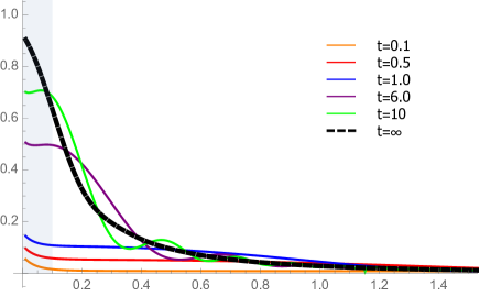
Figure 1: (Color online) Time evolution of the (column-density) momentum distribution function, $\tilde{n}_{{\bf k}_{\perp}}(t)\equiv\int dk_{z}n_{\bf k}(t)$ following a deep scattering length quench $k_{n}a_{i}=0.01\rightarrow k_{n}a_{f}=1$ in a resonant Bose gas (where $k_{n}\equiv n^{1/3}$), computed within a self-consistent dynamic field approximation. Here momentum is rescaled by the coherence length $\xi$ as $\hat{k}=k\xi\equiv k/\sqrt{2mng_{f}}$. Lowest curve corresponds to earlier time at $\hat{t}\equiv t/t_{0}=0.1$ in units of pre-thermalization timescale $t_{0}=1/ng_{f}=m/(4\pi a_{f}n)$ while the dashed-thick black one represents the asymptotic steady-state distribution. The figure illustrates the initial narrow momentum distribution (lowest curve) evolving to a much broader momentum distribution (highest curve), corresponding to a pre-thermalized steady state. The grey region indicates a range of momenta not resolved in JILA experiments, due to initial inhomogeneous real space density profile and finite trap size.

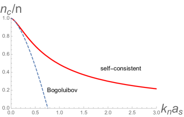
Figure 2: (Color online) Ground state condensate fraction as a function of a dimensionless measure of atom density and interaction, $k_{n}a_{s}$(with $k_{n}\equiv n^{1/3}$), computed within a self-consistent dynamic field approximation (solid red curve), as compared to Bogoluibov approximation result (dashed blue curve).

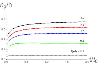
Figure 3: (Color online) Time evolution of the condensate depletion fraction $n_{d}(t)/n$ (treated within a self-consistent dynamic field analysis), following a scattering length quench from $k_{n}a_{i}=0.01$ to various $k_{n}a_{f}$ in a resonant Bose gas. Here we normalize the time with the pre-thermalization timescale $t_{0}=1/ng_{f}=m/(4\pi a_{f}n)$ associated with $k_{n}a_{f}=1$ (where $k_{n}\equiv n^{1/3}$).

We also studied the excitation energy after a constant ramp rate $\gamma$ between $a_{i}$ and $a_{f}$ scattering lengths. As illustrated in Fig. 4, we found that it displays a $\sqrt{\gamma}$ form

$$\frac{E_{exc}(\gamma)}{V} = \frac{4(\sigma-1)^{2}n^{2}a_{f}}{m}a_{f}\Lambda f(\gamma/E_{\Lambda}),$$

$$\propto \mbox{$(1-\sigma)^{3/2}\sqrt{\gamma}$, \;\; for $\gamma\ll E_{\Lambda}$},$$

$$\propto \mbox{$(1-\sigma)^{2}a_{f}\Lambda~{}$,\;\;\;\;\;for $\gamma\gg E_{\Lambda}$},$$

for a ramp-rate below the microscopic energy cutoff $E_{\Lambda}=\Lambda^{2}/2m$.

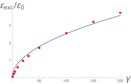
Figure 4: (Color online) Excitation energy (scaled by LHY correction to the ground state energy) following a scattering length ramp as a function of ramp rate $\gamma$ (as a “zoom-in” for Fig. 22, see Sec. VII). The red data points are obtained for each chosen $\gamma$ at $a_{i}/a_{f}={1}/{2}$, with scaled dimensionless momentum cutoff $\hat{\Lambda}=\Lambda\xi=100$ ($\xi\equiv 1/\sqrt{2mng_{f}}$ is the coherence length); the blue curve represents the fitting function $y=0.26\sqrt{x}$.

To further characterize the post-quench evolution and the resulting pre-thermalized steady-state we have also computed a time dependent structure function $S(q,t)=\langle gs_{i}|n(-{\bf q},t)n({\bf q},t)|gs_{i}\rangle$, a Fourier transform of the density-density connected correlation function. For the weakly interacting, shallow-quench regime, at temperature $1/\beta$ it is given by

$$\begin{split}S(q,t)=\frac{n_{0}\epsilon_{q}}{E^{2}_{qf}}\coth(\beta E_{qi}/2)\left[1+\frac{E^{2}_{qi}-E^{2}_{qf}}{E^{2}_{qf}}\sin^{2}(E_{qf}t)\right],\end{split}$$ (6)

first computed and measured in Ref. ChinGurarie13 , and after pre-thermalization reduces to a time-independent form YinLR14 ,

$$\begin{split}S^{ss}_{q}=\frac{n_{0}\epsilon_{q}}{2E^{2}_{qf}}\coth(\beta E_{qi}/2)\left(1+\frac{E^{2}_{qi}}{E^{2}_{qf}}\right).\end{split}$$ (7)

Utilizing our self-consistent dynamic field theory we extended above calculation of $S(q,t)$ to deep quenches of strongly interacting resonant condensates. The resulting time-dependent structure function and its steady-state form are illustrated in Fig. 5.

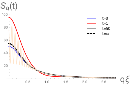
Figure 5: (Color online) Time evolution of the structure function $S_{\bf q}(t)$ defined in the text following a scattering length quench from $0.1a_{f}\to a_{f}$ with $k_{n}a_{f}=0.7$ (where $k_{n}\equiv n^{1/3}$), referring to Eq. (100) using quasi-adiabatic self-consistent approximation (see Sec. VI.1). It illustrates the initial ground state structure function (blue curve), that following the quench develops oscillations and after a pre-thermalization time approaches a steady-state distribution (dashed black curve), which within-quasi-adiabatic approximation almost collapses with the initial ground state curve. Here momentum and time are rescaled with $\xi\equiv 1/\sqrt{2mng_{f}}$ and $t_{0}\equiv 1/(ng_{f})$, respectively.

We also computed the RF spectroscopy signal $I(\omega_{RF})$ JinRF ; Wild , that measures the transition rate of atoms from two resonantly interacting hyperfine states into a third weakly interacting hyperfine state, for the quench process. Within the Bogoluibov approximation the response is given by

$$I(\omega_{RF})=\frac{\sqrt{2}\tau VI^{2}_{0}}{4\sqrt{\pi m}}\frac{(4\pi na_{f})^{2}}{\omega_{RF}^{3/2}},$$ (8)

as measured experimentally, with the amplitude proportional to Tan’s contact, that in the simplest Bogoluibov approximation is given by $C=(4\pi na_{f})^{2}$.

We next turn to a single-channel Feshbach resonant model, followed by its detailed analysis that led to above and other results.

II Model of a resonant superfluid

A resonant gas of bosonic atoms can be modeled by a single-channel grand-canonical Hamiltonian, (defining $\int_{\bf r}\equiv\int d^{3}r$)

$$\begin{split}\hat{H}=\int_{\bf r}[\hat{\psi}^{\dagger}(\hat{\epsilon}-\mu)\hat{\psi}+\frac{g}{2}\hat{\psi}^{\dagger}\hat{\psi}^{\dagger}\hat{\psi}\hat{\psi}],\end{split}$$ (9)

where $\hat{\psi}({\bf r})$ is a bosonic atom field operator, $\hat{\epsilon}=-\frac{\nabla^{2}}{2m}$ is a single-particle Hamiltonian, $\mu$ is the chemical potential, and the pseudo-potential $g$ characterizes the atomic two-body interaction on the scale longer than its microscopic range $r_{0}=1/\Lambda$, typically on the order of ten angstroms. For simplicy, we have set $\hbar=1$.

As discussed in detail in Ref. GurarieRadzihovskyAOP and references therein, near a Feshbach resonance the magnetic field-dependent coupling $g(B)$ controls the s-wave scattering length $a_{s}$ through the renormalized coupling ($T$-matrix) $\tilde{g}^{-1}=g^{-1}+\int_{\bf k}\frac{1}{2\epsilon_{k}}=g^{-1}+m\Lambda/(2\pi^{2})$,

$$\tilde{g}=\frac{g}{1+g/g_{c}},$$ (10)

related to the scattering length via $\tilde{g}=4\pi a_{s}/m$. As illustrated in Fig. 6, for a sufficiently strong attractive interaction, in a vacuum, the two-atom scattering length diverges at $g_{c}=2\pi^{2}/(m\Lambda)=2\pi^{2}r_{0}/m$, as the two-body bound state forms for $g<-g_{c}$ and $a_{s}$ turns positive on the so-called “BEC” side of the Feshbach resonance. $r_{0}$ is the range of the potential and $\Lambda$ is the corresponding momentum cutoff. It is this scattering-length tunability that enables studies of phase transitions in resonant Bose RPWmolecularBECprl04 ; StoofMolecularBEC04 ; RPWmolecularBECpra08 ; ZhouPRA08 ; BonnesWessePRB12 (and BCS-BEC crossover in Fermi GrimmBCS-BEC ; JinBCS-BEC ; ZweirleinReview ; FRrmp ; BlochRMP ; ZweirleinReview ; GurarieRadzihovskyAOP ) gases and quenched dynamics ChinGurarie13 ; Makotyn ; YinLR14 ; SykesPRA14 that is our focus here.

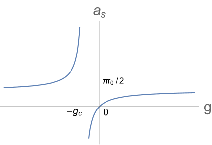
Figure 6: (Color online) A plot of the s-wave scattering length $a_{s}$ (renormalized coupling $\tilde{g}$) as a function of bare coupling $g$ in a Feshbach resonance. Here $g_{c}=2\pi^{2}r_{0}/m$ is the critical coupling strength at which $a_{s}$ diverges.

To allow for dynamics within a Bose-condensed state explored experimentally ChinGurarie13 ; Makotyn , we decompose the atomic field operator $\hat{\psi}({\bf r})=\frac{1}{\sqrt{V}}\sum_{\bf k}\hat{a}_{\bf k}e^{i{\bf k}\cdot{\bf r}}$, into a c-field condensate $\Psi_{0}$ and a fluctuation field $\hat{a}({\bf r})$,

$$\begin{split}\hat{\psi}=\Psi_{0}+\hat{a}.\end{split}$$ (11)

Expressing the Hamiltonian, (9) in terms of the operator $\hat{a}$, it decomposes into

$$\begin{split}\hat{H}=\hat{H}_{0}+\hat{H}_{1}+\hat{H}_{2}+\hat{H}_{3}+\hat{H}_{4},\end{split}$$ (12)

where

$$\begin{split}\hat{H}_{0}=\int_{\bf r}[\Psi_{0}^{*}(\hat{\epsilon}-\mu)\Psi_{0}+\frac{g}{2}|\Psi_{0}|^{4}],\end{split}$$ (13)

is the lowest order mean-field ground-state energy, and

$$\begin{split}\hat{H}_{1}=\int_{\bf r}[\hat{a}^{\dagger}(\hat{\epsilon}+g|\Psi_{0}|^{2}-\mu)\Psi_{0}]+h.c.,\\ \end{split}$$ (14a)

$$\begin{split}\hat{H}_{2}=\int_{\bf r}\left[\hat{a}^{\dagger}\left(\hat{\epsilon}+2g|\Psi_{0}|^{2}-\mu\right)\hat{a}+\frac{g}{2}\left({\Psi_{0}^{*}}^{2}\hat{a}\hat{a}+\Psi_{0}^{2}\hat{a}^{\dagger}\hat{a}^{\dagger}\right)\right],\end{split}$$ (14b)

$$\begin{split}\hat{H}_{3}=g\int_{\bf r}[\Psi_{0}\hat{a}^{\dagger}\hat{a}^{\dagger}\hat{a}+\Psi_{0}^{*}\hat{a}^{\dagger}\hat{a}\hat{a}],\end{split}$$ (14c)

$$\begin{split}\hat{H}_{4}=\frac{g}{2}\int_{\bf r}\hat{a}^{\dagger}\hat{a}^{\dagger}\hat{a}\hat{a}.\end{split}$$ (14d)

are the operator components organized by respective orders in the excitation $\hat{a}$.

II.1 Bogoluibov approximation for weakly interacting bosons

We set the stage for the study of dynamics following a shallow quench ChinGurarie13 and of a self-consistent dynamic field treatment YinLR14 of a deep quench Makotyn by first briefly summarizing the results for the ground state and excitations in the Bogoluibov approximation Bogoliubov ; Fetter .

In the weakly interacting limit the atomic gas is characterized by a small gas parameter $na_{s}^{3}\ll 1$, well-approximated by the Bogoluibov quadratic Hamiltonian, neglecting the nonlinear $\hat{H}_{3,4}$ components of $\hat{H}$. Focusing on the uniform (bulk) condensate and eliminating the chemical potential in favor the condensate density by requiring the vanishing of the $\hat{H}_{1}$ component (equivalent to a minimization of $\hat{H}_{0}$ over $\Psi_{0}$), $\mu=g|\Psi_{0}|^{2}\approx gn$, neglecting the difference between the condensate density, $|\Psi_{0}|^{2}\equiv n_{c}$ and total atom density, $n$, the grand-canonical Hamiltonian reduces to $\hat{H}\approx-{\frac{1}{2}}Vgn^{2}+\hat{H}_{B}$,

$$\hat{H}_{B} = -{\frac{1}{2}}\sum_{{\bf k}\neq 0}\varepsilon_{k}+{\frac{1}{2}}\sum_{{\bf k}\neq 0}\begin{pmatrix}\hat{a}_{\bf k}^{\dagger}&\hat{a}_{-{\bf k}}\\ \end{pmatrix}\begin{pmatrix}\varepsilon_{k}&gn_{c}\\ gn_{c}&\varepsilon_{k}\\ \end{pmatrix}\begin{pmatrix}\hat{a}_{\bf k}\\ \hat{a}_{-{\bf k}}^{\dagger}\\ \end{pmatrix},$$ (15)

$$= -{\frac{1}{2}}\sum_{{\bf k}\neq 0}\varepsilon_{k}+{\frac{1}{2}}\sum_{{\bf k}\neq 0}\hat{\Phi}^{\dagger}_{{\bf k},i}h_{{\bf k},ij}\hat{\Phi}_{{\bf k},j},$$

$$= -{\frac{1}{2}}\sum_{{\bf k}\neq 0}\varepsilon_{k}+{\frac{1}{2}}\sum_{{\bf k}\neq 0}E_{k}\hat{\Psi}^{\dagger}_{{\bf k},s}\hat{\Psi}_{{\bf k},s},$$

$$= -{\frac{1}{2}}\sum_{{\bf k}\neq 0}(\varepsilon_{k}-E_{k})+\sum_{{\bf k}\neq 0}E_{k}\hat{\alpha}_{\bf k}^{\dagger}\hat{\alpha}_{\bf k},$$

where the quadratic Hamiltonian was straightforwardly diagonalized in terms of the Bogoluibov quasi-particles $\hat{\Psi}_{\bf k}=(\hat{\alpha}_{\bf k},\hat{\alpha}_{-{\bf k}}^{\dagger})$, related to the atomic Nambu spinor $\hat{\Phi}_{\bf k}=(\hat{a}_{\bf k},\hat{a}_{-{\bf k}}^{\dagger})$ by a pseudo-unitary transformation, $U_{\bf k}$

$$\begin{pmatrix}\hat{a}_{\bf k}\\ \hat{a}_{-{\bf k}}^{\dagger}\\ \end{pmatrix} = \begin{pmatrix}u_{\bf k}&v_{\bf k}\\ v^{*}_{\bf k}&u^{*}_{\bf k}\\ \end{pmatrix}\begin{pmatrix}\hat{\alpha}_{\bf k},\\ \hat{\alpha}_{-{\bf k}}^{\dagger},\\ \end{pmatrix}$$ (16a)

$$\hat{\Phi}_{\bf k} = U_{\bf k}\hat{\Psi}_{\bf k}.$$ (16b)

$U_{\bf k}$ satisfies a pseudo eigenvalue equation $h_{\bf k}U_{\bf k}=E_{\bf k}\sigma^{z}U_{\bf k}$ and preserves the canonical commutation relation, $[a_{\bf k},a_{{\bf k}^{\prime}}^{\dagger}]=\delta_{{\bf k},{\bf k}^{\prime}}$, corresponding to $[\hat{\Phi}_{i{\bf k}},\hat{\Phi}^{\dagger}_{j{\bf k}^{\prime}}]=\sigma^{z}_{ij}\delta_{{\bf k},{\bf k}^{\prime}}$, defined by

$$U\sigma_{z}U^{\dagger}=\sigma_{z},$$ (17)

with $|u_{\bf k}|^{2}-|v_{\bf k}|^{2}=1$ and $\sigma^{z}$ the third Pauli matrix.

With $\varepsilon_{k}=k^{2}/2m+gn$ in (15), the Bogoluibov spectrum is given by a well-known gapless form,

$$E_{k} = \sqrt{\varepsilon_{k}^{2}-g^{2}n^{2}}=\sqrt{\epsilon_{k}^{2}+2gn\epsilon_{k}}=ck\sqrt{1+\xi^{2}k^{2}/2},$$

that interpolates between the low-momentum zeroth-sound with velocity $c=\sqrt{gn/m}$ (a Goldstone mode of the $U(1)$ symmetry breaking) and the high-momentum quadratic dispersion, with crossover scale set by the correlation length $\xi=1/\sqrt{2mgn}$. The corresponding coherence factors defining $U_{\bf k}$ are given by

$$u_{k}^{2} = {\frac{1}{2}}\left(\frac{\varepsilon_{k}}{E_{k}}+1\right),\ \ v_{k}^{2}={\frac{1}{2}}\left(\frac{\varepsilon_{k}}{E_{k}}-1\right).$$ (19)

The ground state is a vacuum of Bogoluibov quasi-particles, $\hat{\alpha}_{\bf k}|gs\rangle=0$, with the energy density ${\cal E}_{gs}=V^{-1}\langle gs|\hat{H}|gs\rangle$ given by

$${\cal E}_{gs} = {\frac{1}{2}}gn^{2}-\frac{1}{V}\sum_{{\bf k}\neq 0}E_{k}n_{k},$$ (20a)

$$= \frac{2\pi a_{s}}{m}n^{2}\left[1+\frac{128}{15\sqrt{\pi}}(na^{3}_{s})^{1/2}\right],$$ (20b)

where the $T=0$ momentum distribution function

$$n_{k} = \langle gs|\hat{a}_{k}^{\dagger}\hat{a}_{k}|gs\rangle=|v_{k}|^{2}\approx_{k\rightarrow\infty}C/k^{4},$$ (21)

with Tan’s contact $C=\partial{\cal E}_{gs}/\partial a^{-1}_{s}=16\pi^{2}n^{2}a^{2}_{s}[(1+\frac{64}{3\sqrt{\pi}}(na^{3}_{s})^{1/2}]$ and

$$\mu = \frac{4\pi an}{m}\left[1+\frac{32}{3\sqrt{\pi}}(na^{3}_{s})^{1/2}\right].$$ (22)

The interaction-driven condensate depletion, $n_{d}\equiv n-n_{c}$ is given by

$$n_{d} = \frac{1}{V}\sum_{\bm{k}\neq 0}n_{k}\approx\frac{8}{3\sqrt{\pi}}\left(na^{3}_{s}\right)^{1/2}n,$$ (23)

and provides an important measure of the validity of the Bogoluibov approximation that neglects the difference between $n$ and $n_{c}$.

Clearly, for a large gas parameter, $na^{3}_{s}\gg 1$ the depletion is substantial and must be accounted for. Although there is no currently available systematic analysis in this nonperturbative limit, as we will show in subsequent sections, an uncontrolled self-consistent method, akin to a spherical, large-$N$ model ZinnJustin ; ChaikinLubensky ; SotiriadisCardy10 ; Sondhi13 ; LRunpublished captures important qualitative physics in this resonantly interacting regime.

II.2 Generalization for large scattering length

To extend the analysis to a large $na^{3}_{s}$ we need to account (even if approximately) for the nonlinear components of the Hamiltonian, $\hat{H}_{3,4}$ neglected in the Bogoluibov model. To this end, in the spirit of variational theory or a spherical model ChaikinLubensky , we replace these nonlinear operators by their “best” approximation in terms of operators up to a quadratic order in fluctuation field $\hat{a}$. Using Wick’s theorem, we have

$$\hat{a}^{\dagger}\hat{a}^{\dagger}\hat{a}\hat{a} \rightarrow 4\langle\hat{a}^{\dagger}\hat{a}\rangle\hat{a}^{\dagger}\hat{a}+\langle\hat{a}^{\dagger}\hat{a}^{\dagger}\rangle\hat{a}\hat{a}+\langle\hat{a}\hat{a}\rangle\hat{a}^{\dagger}\hat{a}^{\dagger}$$ (24a)

$$-2\langle\hat{a}^{\dagger}\hat{a}\rangle\langle\hat{a}^{\dagger}\hat{a}\rangle-\langle\hat{a}^{\dagger}\hat{a}^{\dagger}\rangle\langle\hat{a}\hat{a}\rangle,$$

$$\approx 4n_{d}\hat{a}^{\dagger}\hat{a}-2n_{d}^{2},$$

$$\hat{a}^{\dagger}\hat{a}\hat{a} \rightarrow 2\langle\hat{a}^{\dagger}\hat{a}\rangle\hat{a}\approx 2n_{d}\hat{a},$$ (24b)

$$\hat{a}^{\dagger}\hat{a}^{\dagger}\hat{a} \rightarrow 2\hat{a}^{\dagger}\langle\hat{a}^{\dagger}\hat{a}\rangle\approx 2n_{d}\hat{a}^{\dagger},$$ (24c)

where we kept the depletion density $n_{d}=\langle\hat{a}^{\dagger}\hat{a}\rangle$ and neglected “anomalous” averages (e.g., $\langle\hat{a}\hat{a}\rangle=0$) and high order correlators (e.g., $\langle\hat{a}^{\dagger}\hat{a}\hat{a}\rangle=0$) that we expect to be subdominant.

With these we approximate $\hat{H}_{3}$ and $\hat{H}_{4}$ by a linear and quadratic forms

$$\hat{H}_{3} = g\int_{\bf r}[\Psi_{0}\hat{a}^{\dagger}\hat{a}^{\dagger}\hat{a}+\Psi_{0}^{*}\hat{a}^{\dagger}\hat{a}\hat{a}]\to\delta\hat{H}_{1},$$ (25)

where

$$\delta\hat{H}_{1} = g\int_{\bf r}(2\Psi_{0}n_{d}\hat{a}^{\dagger}+h.c.),$$ (26)

and

$$\hat{H}_{4} = \frac{g}{2}\int_{\bf r}\hat{a}^{\dagger}\hat{a}^{\dagger}\hat{a}\hat{a}\to\delta\hat{H}_{0}+\delta\hat{H}_{2},$$ (27)

where

$$\delta\hat{H}_{0} = -gVn_{d}^{2},$$ (28a)

$$\delta\hat{H}_{2} = 2g\int_{\bf r}n_{d}\hat{a}^{\dagger}\hat{a}.$$ (28b)

The grand-canonical Hamiltonians now take the following forms: $\hat{H}\approx\hat{H}^{\prime}_{0}+\hat{H}^{\prime}_{1}+\hat{H}^{\prime}_{2}$, where

$$\begin{split}\hat{H}^{\prime}_{0}&=\hat{H}_{0}+\delta\hat{H}_{0},\\ &=\int_{\bf r}\left[\Psi_{0}^{*}(\hat{\epsilon}-\mu)\Psi_{0}+\frac{g}{2}n^{2}_{c}-gn^{2}_{d}\right],\end{split}$$ (29a)

$$\begin{split}\hat{H}^{\prime}_{1}&=\hat{H}_{1}+\delta\hat{H}_{1},\\ &=\int_{\bf r}\left[\hat{a}^{\dagger}(\hat{\epsilon}+gn_{c}+2gn_{d}-\mu)\Psi_{0}\right]+h.c.,\end{split}$$ (29b)

$$\begin{split}\hat{H}^{\prime}_{2}&=\hat{H}_{2}+\delta\hat{H}_{2},\\ &=\int_{\bf r}\left[\hat{a}^{\dagger}(\hat{\epsilon}+2g(n_{c}+n_{d})-\mu)\hat{a}+\frac{gn_{c}}{2}(\hat{a}\hat{a}+\hat{a}^{\dagger}\hat{a}^{\dagger})\right].\end{split}$$ (29c)

Above, for simplicity, we have defined $n_{c}\equiv|\Psi_{0}|^{2}$ and $n_{d}\equiv\langle\hat{a}^{\dagger}\hat{a}\rangle$ and in Eqs. (29a),(29b),(29c) have discarded the ”anomalous average” term $\tilde{m}\equiv\langle\hat{a}\hat{a}\rangle$ to satisfy the constraint of Goldstone theorem, which requires a gapless excitation spectrum. This amounts to the widely used Popov approximation HFB_Popov .

Following what was done in the last subsection, we fix the chemical potential $\mu$ by requiring $\hat{H}^{\prime}_{1}=0$

$$\begin{split}(\hat{\epsilon}+g|\Psi_{0}|^{2}+2gn_{d})\Psi_{0}=\mu\Psi_{0}.\end{split}$$ (30)

For a uniform system, this gives

$$\begin{split}\mu=gn_{c}+2gn_{d}.\end{split}$$ (31)

Thus we obtain the grand-canonical Hamiltonian

$$\begin{split}\hat{H}&=\int_{\bf r}\left[\hat{a}^{\dagger}(\hat{\epsilon}+gn_{c})\hat{a}+\frac{g}{2}n_{c}(\hat{a}\hat{a}+\hat{a}^{\dagger}\hat{a}^{\dagger})\right]-E_{0}\\ &=\sum_{\bm{k}\neq 0}\left[(\epsilon_{k}+gn_{c})\hat{a}^{\dagger}_{\bf k}\hat{a}_{\bf k}+\frac{1}{2}gn_{c}(\hat{a}^{\dagger}_{\bf k}\hat{a}^{\dagger}_{-{\bf k}}+\hat{a}_{\bf k}\hat{a}_{-{\bf k}})\right]-E_{0},\end{split}$$ (32)

where $E_{0}/V=\frac{g}{2}n^{2}_{c}+2gn_{c}n_{d}+gn_{d}^{2}$. It exhibits the standard Bogoluibov form with gapless spectrum, but also approximately accounts for a potentially strong depletion through the condensate density $n_{c}$ replacing the full density $n$ as the self-consistently determined parameter of the Hamiltonian.

III self-consistent analysis for strongly interacting ground state

Before turning to our main focus of nonequilibrium post-quench dynamics, we examine the ground state properties of a strongly interacting resonant Bose gas, characterized by a large scattering length and gas parameter $na^{3}_{s}\gg 1$. This regime lies beyond the scope of the standard Bogoluibov theory. Nevertheless we expect to be able to treat it qualitatively correctly (even if quantitatively uncontrolled) by taking into account the large depletion $n-n_{c}>0$ through the Hamiltonian (32) and the self-consistency condition through the atom number conservation

$$n = n_{c}+\frac{1}{V}\sum_{\bm{k}\neq 0}\langle\hat{a}^{\dagger}_{\bf k}\hat{a}_{\bf k}\rangle,$$ (33a)

$$= n_{c}+\frac{8}{3\sqrt{\pi}}\left({n_{c}a^{3}_{s}}\right)^{1/2}n_{c},$$ (33b)

where in the second line we calculated the depletion by diagonalizing (32) as in Sec. II.1 of the conventional Bogoluibov theory, but with $n_{c}$ replacing $n$. Such treatment is quite close in spirit to the self-consistent Hartree-Fock approximations, and the BCS and other mean-field gap equations.

In the dimensionless form for $\hat{n}_{c}=n_{c}/n$, the self-consistency equation reduces to

$$\begin{split}1-\hat{n}_{c}-\lambda{\hat{n}}^{3/2}_{c}=0,\end{split}$$ (34)

where $\lambda=8(na^{3}_{s})^{1/2}/(3\sqrt{\pi})\equiv 8(k_{n}a_{s})^{3/2}/(3\sqrt{\pi})$, with $k_{n}\equiv n^{1/3}$ the mometum scale set by the boson density $n$.

The solution to Eq. (34) is illustrated in Fig. 2. We find that the self-consistency constraint suppresses condensate depletion, leading to a higher condensate fraction $n_{c}$ than the Bogoluibov approximation for the same strength of the interaction parameter $k_{n}a_{s}$. We also observe that, as expected the correction to Bogoluibov theory from the self-consistency condition grows (from zero) with increasing gas parameter $k_{n}a_{s}$, thereby avoiding the spurious transition to a vanishing condensate state appearing in the Bogoluibov theory.

IV Dynamics for shallow quench

We now turn to nonequilibrium dynamics following a change in the scattering length $a_{s}$ from its initial value $a_{i}$ to the final value $a_{f}$, as can be realized experimentally in a Feshbach resonant Bose gas by a change in the external magnetic field Makotyn . Here we assume the change is instantaneous (sudden quench), allowing analytical analysis. In this section, we focus on shallow quenches characterized by both $na^{3}_{i}\ll 1$ and $na^{3}_{f}\ll 1$, so that the Bogoluibov approximation remains rigorously valid.

For shallow quenches, the system is well approximated by Hamiltonian (15) with $g_{i}$ and $g_{f}$ for the initial and final Hamiltonians, respectively, with corresponding Bogoluibov quasi-particle bases $(\hat{\alpha}_{\bf k},\hat{\alpha}^{\dagger}_{\bf k})$ prior to the quench and $(\hat{\beta}_{\bf k},\hat{\beta}^{\dagger}_{\bf k})$ post the quench. Focussing on a sudden quench, the two sets of bases are related to the atomic basis $(\hat{a}_{\bf k},\hat{a}^{\dagger}_{\bf k})$ via a pseudo-unitary transformations

$$\begin{pmatrix}\hat{a}_{\bf k}\\ \hat{a}^{\dagger}_{-{\bf k}}\end{pmatrix} = \begin{pmatrix}u^{\prime}_{k}&v^{\prime}_{k}\\ v^{\prime}_{k}&u^{\prime}_{k}\end{pmatrix}\begin{pmatrix}\hat{\alpha}_{\bf k}\\ \hat{\alpha}^{\dagger}_{-{\bf k}}\end{pmatrix},$$ (35a)

$$\hat{\Phi}_{\bf k}(0) = U_{k}(0^{-})\hat{\Psi}_{{\bf k}}(0^{-}),$$ (35b)

and

$$\begin{pmatrix}\hat{a}_{\bf k}\\ \hat{a}^{\dagger}_{-{\bf k}}\end{pmatrix} = \begin{pmatrix}u_{k}&v_{k}\\ v_{k}&u_{k}\end{pmatrix}\begin{pmatrix}\hat{\beta}_{\bf k}\\ \hat{\beta}^{\dagger}_{-{\bf k}}\end{pmatrix},$$ (36a)

$$\hat{\Phi}_{\bf k}(0) = U_{k}(0^{+})\hat{\Psi}_{{\bf k}}(0^{+}),$$ (36b)

where

$$u^{\prime}_{k} = \sqrt{\frac{1}{2}\left(\frac{\epsilon_{k}+ng_{i}}{E_{ki}}+1\right)},\;\;v^{\prime}_{k}=-\sqrt{\frac{1}{2}\left(\frac{\epsilon_{k}+ng_{i}}{E_{ki}}-1\right)},$$

$$u_{k} = \sqrt{\frac{1}{2}\left(\frac{\epsilon_{k}+ng_{f}}{E_{kf}}+1\right)},\;\;v_{k}=-\sqrt{\frac{1}{2}\left(\frac{\epsilon_{k}+ng_{f}}{E_{kf}}-1\right)},$$

define Bogoluibov transformations for Hamiltonians $\hat{H}_{i}$ (with interaction $g_{i}\equiv g(0^{-})$) before and $\hat{H}_{f}$ (with interaction $g_{f}\equiv g(0^{+})$) after the quench, respectively. The corresponding excitation spectra are

$$E_{ki}=\sqrt{{\epsilon_{k}}^{2}+2ng_{i}\epsilon_{k}},\;\;E_{kf}=\sqrt{{\epsilon_{k}}^{2}+2ng_{f}\epsilon_{k}},$$ (38)

and the two quasi-particle bases are related by

$$\begin{pmatrix}\hat{\beta}_{\bf k}\\ \hat{\beta}^{\dagger}_{-{\bf k}}\end{pmatrix} = U_{k}^{-1}(0^{+})U_{k}(0^{-})\begin{pmatrix}\hat{\alpha}_{\bf k}\\ \hat{\alpha}^{\dagger}_{-{\bf k}}\end{pmatrix},$$ (39)

$$= \begin{pmatrix}\cosh\Delta\theta_{k}&\sinh\Delta\theta_{k}\\ \sinh\Delta\theta_{k}&\cosh\Delta\theta_{k}\end{pmatrix}\begin{pmatrix}\hat{\alpha}_{\bf k}\\ \hat{\alpha}^{\dagger}_{-{\bf k}}\end{pmatrix},$$

with

$$\Delta\theta_{k}=\frac{1}{2}\cosh^{-1}\left[{\frac{1}{2}}\left(\frac{E_{kf}}{E_{ki}}+\frac{E_{ki}}{E_{kf}}\right)\right].$$ (40)

We take the initial state $|0^{-}\rangle$ to be the ground state of the pre-quenched Hamiltonian $\hat{H}_{i}$ footnote , and thus a vacuum of $\hat{\alpha}$ quasi-particles, $\hat{\alpha}_{\bf k}|0^{-}\rangle=0$. At finite temperature this generalizes to Bose-Einstein distribution of $\hat{\alpha}$ quasi-particle occupation,

$$\langle\hat{\alpha}^{\dagger}_{{\bf k}}\hat{\alpha}_{\bf k}\rangle_{0^{-}}=\frac{1}{e^{E_{ki}/T}-1}.$$ (41)

Because experiments probe physical observables expressed in terms of atomic operators, we need to compute time evolution of $\hat{\Phi}_{\bf k}(t)=(\hat{a}_{\bf k}(t),\hat{a}^{\dagger}_{\bf k}(t))$. Using free post-quench evolution of $\hat{\beta}$ quasi-particles

$$\begin{pmatrix}\hat{\beta}_{\bf k}(t)\\ \hat{\beta}^{\dagger}_{-{\bf k}}(t)\end{pmatrix}=\begin{pmatrix}e^{-iE_{kf}t}&0\\ 0&e^{iE_{kf}t}\end{pmatrix}\begin{pmatrix}\hat{\beta}_{\bf k}(0)\\ \hat{\beta}^{\dagger}_{-{\bf k}}(0)\end{pmatrix}\equiv T_{k}(t)\hat{\Psi}_{\bf k}(0^{+}),$$ (42)

the relation (39), together with the simplicity of matrix elements of $\hat{\alpha}$ quasi-particles in the pre-quench ground state (vacuum of $\hat{\alpha}_{\bf k}$), we find

$$\begin{pmatrix}\hat{a}_{\bf k}(t)\\ \hat{a}^{\dagger}_{-{\bf k}}(t)\end{pmatrix} = U_{k}(0^{+})\begin{pmatrix}\hat{\beta}_{\bf k}(t)\\ \hat{\beta}^{\dagger}_{-{\bf k}}(t)\end{pmatrix},$$ (43a)

$$= U_{k}(0^{+})T_{k}(t)\begin{pmatrix}\hat{\beta}_{\bf k}(0)\\ \hat{\beta}^{\dagger}_{-{\bf k}}(0)\end{pmatrix},$$

$$= U_{k}(0^{+})T_{k}(t)U_{k}^{-1}(0^{+})U_{k}(0^{-})\begin{pmatrix}\hat{\alpha}_{\bf k}(0)\\ \hat{\alpha}^{\dagger}_{-{\bf k}}(0)\end{pmatrix},$$

$$\hat{\Phi}_{\bf k}(t) = U_{k}(t)\hat{\Psi}_{{\bf k}}(0^{-})=R_{k}(t)U_{k}(0^{-})\hat{\Psi}_{{\bf k}}(0^{-}),$$

where the matrix

$$R_{ij}(t) = U_{il}T_{lm}(t)U_{mn}^{-1},$$

$$= (\cos E_{kf}t)I_{ij}+i\frac{\sin E_{kf}t}{E_{kf}}\begin{pmatrix}\epsilon_{k}+g_{f}n&g_{f}n\\ -g_{f}n&-\epsilon_{k}-g_{f}n\\ \end{pmatrix},$$

evolves the initial Bogoluibov spinor $\left(u_{k}(0^{-}),v_{k}(0^{-})\right)\rightarrow\left(u_{k}(t),v_{k}(t)\right)$, and

$$U_{k}(t) = U_{k}(0^{+})T_{k}(t)U_{k}^{-1}(0^{+})U_{k}(0^{-}),$$

$$= \begin{pmatrix}u_{k}e^{-iE_{kf}t}&v_{k}e^{iE_{kf}t}\\ v_{k}e^{-iE_{kf}t}&u_{k}e^{iE_{kf}t}\end{pmatrix}\begin{pmatrix}\cosh\Delta\theta_{k}&\sinh\Delta\theta_{k}\\ \sinh\Delta\theta_{k}&\cosh\Delta\theta_{k}\end{pmatrix}.$$

Having derived the evolution of the atomic fields $\hat{\Phi}_{\bf k}(t)=(\hat{a}_{\bf k}(t),\hat{a}^{\dagger}_{\bf k}(t))$, we can now compute the basic atomic bilinear correlator (supressing the momentum ${\bf k}$ argument on the right hand-side):

$$C_{\bf k}^{ij}(t,t^{\prime}) = \langle\hat{\Phi}_{i}^{\dagger}(t)\hat{\Phi}_{j}(t^{\prime})\rangle,$$ (46)

$$= \langle\hat{\Psi}^{\dagger}_{m}(0^{-})U^{\dagger}_{mi}(t)U_{jn}(t^{\prime})\hat{\Psi}_{n}(0^{-})\rangle,$$

$$= U^{\dagger}_{mi}(t)N_{mn}U_{jn}(t^{\prime}),$$

in terms of the pre-quench ($t=0^{-}$) quasi-particle occupation matrix

$$N_{mn} = \langle\hat{\Psi}^{\dagger}_{m}(0^{-})\hat{\Psi}_{n}(0^{-})\rangle,$$ (47a)

$$= \begin{pmatrix}\langle\hat{\alpha}^{\dagger}_{\bf k}\hat{\alpha}_{\bf k}\rangle&\langle\hat{\alpha}^{\dagger}_{\bf k}\hat{\alpha}^{\dagger}_{-{\bf k}}\rangle\\ \langle\hat{\alpha}_{-{\bf k}}\hat{\alpha}_{\bf k}\rangle&\langle\hat{\alpha}_{-{\bf k}}\hat{\alpha}^{\dagger}_{-{\bf k}}\rangle\\ \end{pmatrix}_{mn},$$ (47b)

$$= \begin{pmatrix}n_{k}(0^{-})&0\\ 0&n_{-k}(0^{-})+1\\ \end{pmatrix}_{mn},$$ (47c)

$$= \begin{pmatrix}0&0\\ 0&1\\ \end{pmatrix}_{mn},\ \ \text{for $T=0$},$$ (47d)

from which physical observables, such as the momentum distribution function, structure function, RF spectroscopy signal, and many others can be obtained. We turn to their computation in the following subsections.

IV.1 Time of flight: momentum distribution function

Time of flight measurements, where a gas is released from its trap and its density profile is measured at long times, is one of the central experimental probes dating back to the realization of BEC in dilute alkali gases CornellWiemannBEC1995 ; KetterleBEC1995 . A straightforward analysis demonstrates RSpolarized , that at long times the density profile is proportional to the momentum distribution function. At $T=0$, that is our main focus here, we obtain

$$n_{k}(t) = \langle 0^{-}|\hat{a}^{\dagger}_{\bf k}(t)\hat{a}_{\bf k}(t)|0^{-}\rangle=C_{k}^{11}(t,t),$$ (48)

$$= |(u_{k}e^{-iE_{kf}t}\sinh\Delta\theta_{k}+v_{k}e^{iE_{kf}t}\cosh\Delta\theta_{k})|^{2},$$

$$= \frac{\epsilon_{k}+g_{i}n+\frac{2g_{f}(g_{f}-g_{i})n^{2}}{\epsilon_{k}+2g_{f}n}\sin^{2}(E_{kf}t)}{2\sqrt{\epsilon_{k}(\epsilon_{k}+2g_{i}n)}}-\frac{1}{2},\quad\quad\quad$$

at $t=0$ reducing to the ground-state momentum distribution Eq. (21), as expected by continuity of evolution. Rescaling momentum as $\hat{k}=k\xi\equiv k/\sqrt{2mng_{f}}$ and time as $\hat{t}=t/t_{0}\equiv tng_{f}$, we obtain the momentum distribution in terms of dimensionless variables as

$$\begin{split}n_{\hat{k}}(\hat{t})=\frac{[\hat{k}^{2}+\sigma+\frac{2(1-\sigma)}{\hat{k}^{2}+2}\sin^{2}(\hat{t}\sqrt{\hat{k}^{2}(\hat{k}^{2}+2)})]}{2\sqrt{\hat{k}^{2}(\hat{k}^{2}+2\sigma)}}-\frac{1}{2},\\ \end{split}$$ (49)

where the initial-to-final scattering length ratio, $\sigma\equiv a_{i}/a_{f}$ characterizes the “depth” of the quench.

The column momentum distribution $\tilde{n}_{\hat{k}}(\hat{t})\equiv\int d\hat{k}_{z}n_{\hat{k}}(\hat{t})$ is a more experimentally relevant quantity that we plot at different times in Fig. 7.

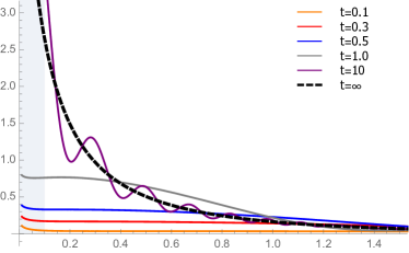
Figure 7: (Color online) Time evolution of the column momentum distribution defined in the text following a scattering length quench from $0.1a_{f}\to a_{f}$, referring to Eq. (49) using Bogoluibov approximation. It illustrates the initial narrow momentum distribution (lowest curve) evolving to a much broader momentum distribution (highest curve), corresponding to a pre-thermalized steady state. Here momentum and time are rescaled with $\xi\equiv 1/\sqrt{2mng_{f}}$ and $t_{0}\equiv 1/(ng_{f})$, respectively. The grey region indicates a range of momenta not resolved in JILA experiments, due to initial inhomogeneous real space density profile and finite trap size.

We observe that starting with a narrow BEC peak, the column momentum distribution function quickly broadens and develops a large momentum tail. The momentum distribution approaches a pre-thermalized steady-state $\tilde{n}^{ss}_{k}$ from high momenta, with momenta $k>k_{pth}(t)$ taking time $t_{pth}(k)\approx 1/E_{kf}$ to pre-thermalize footnote . Thus we obtain

$$\begin{split}t_{pth}(\hat{k})=1/\sqrt{\hat{k}^{2}(\hat{k}^{2}+2)},\end{split}$$ (50)

consistent with experiments Makotyn scaling as $1/k$ and $1/k^{2}$ at small and large momenta, respectively.

The steady-state momentum distribution, $n^{ss}_{k}$ for a $a_{i}=0.1a_{f}\rightarrow a_{f}$ is plotted in Fig. 8 and compared to the ground state $n_{k}$ for the same $a_{f}$ as well as thermal state $n_{k}$ at finite temperature. We observe that this steady-state momentum distribution lies above the ground state one, indicating that even in the long time limit the post-quench system remains in the excited states, as required by energy conservation. However, it also differs significantly from the corresponding finite-temperature thermal-equilibrium distribution, $n^{T}_{k}=(u^{2}_{k}+v^{2}_{k})\langle\hat{\alpha}^{\dagger}_{{\bf k}}\hat{\alpha}_{\bf k}\rangle_{0^{-}}+v^{2}_{k}=1/(e^{E_{kf}/T}-1)+v_{k}^{2}\coth(E_{kf}/2T)$, demonstrating that even in the long time, stationary state limit the system is only pre-thermalized. This is expected because of the quadratic, fully integrable form of the Bogoluibov Hamiltonian. The latter guarantees the absence of scattering of the Bogoluibov quasi-particles $\hat{\beta}_{\bf k}$, with a conserved momentum distribution function, that is directly related to the initial distribution by (39).

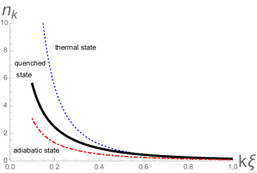
Figure 8: (Color online) Quenched steady-state momentum distribution function $n^{ss}_{k}$ following a scattering length quench $a_{i}=0.1a_{f}\to a_{f}$ (thick black curve), as compared to the ground state momentum distribution at $a_{f}$ (dash-dotted red) and the corresponding Bogoluibov thermalized distribution (dotted blue) at temperature $T=0.45ng_{f}$.

A simpler measure of the post-quench dynamics is the evolution of the condensate depletion, obtained from the momentum distribution function, $n_{k}(t)$, (48),

$$n_{d}(t) = \sum_{\bf k}n_{k}(t)=V\int\frac{d^{3}k}{(2\pi)^{3}}n_{k}(t),$$ (51)

$$= n^{0}_{d}F_{d}(\sigma,t),$$

where $n^{0}_{d}=8/(3\sqrt{\pi})(na_{f}^{3})^{1/2}$ is the ground-state depletion for $a_{s}=a_{f}$.

$$F_{d}(\sigma,t) = (\sigma)^{3/2}+\frac{3}{2}\sqrt{1-\sigma}\mathrm{Arccos}(\sqrt{\sigma})$$ (52)

$$- \frac{3\sqrt{2}}{2}\int ydy\frac{(1-\sigma)\cos(2ty\sqrt{y^{2}+2})}{(y^{2}+2)(y^{2}+2\sigma)^{1/2}}\ \ \ \ \ \ \ \$$

is the nonequilibrium depletion enhancement factor above the corresponding ground state, that interpolates between $\sigma^{3/2}$ (giving the initial depletion at $t=0^{-}$ for $a_{s}=a_{i}$) and the asymptotic depletion

$$\begin{split}F^{ss}_{d}(\sigma)\equiv F_{d}(\sigma,t\to\infty)=\sigma^{3/2}+\frac{3}{2}\sqrt{1-\sigma}\mathrm{Arccos}(\sqrt{\sigma})\end{split}$$ (53)

of the pre-thermalized state, plotted in Fig. 10.

As is clear from the asymptotics of $F_{d}(\sigma,t)$ defined by (53) and illustrated in Fig. 9, the depletion fraction monotonically increases as $\sqrt{t}$ over a characteristic time

$$t_{pth}\approx\frac{1}{ng_{f}},$$ (54)

approaching its asymptotic pre-thermalized value, that is always higher than that of the ground state with the same scattering length $a_{s}=a_{f}$.

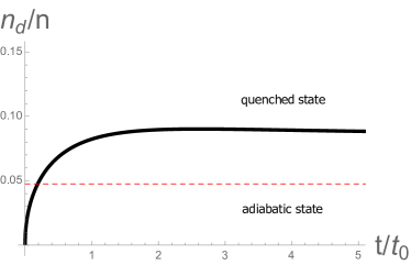
Figure 9: (Color online) Post quench dynamics of the condensate depletion fraction as a function of rescaled time in units of pre-thermalization timescale $t_{0}=\hbar/(ng_{f})=m/(4\pi a_{f}n\hbar)$ (solid black curve), following a scattering length quench from $0.1a_{f}\to a_{f}$ with $k_{n}a_{f}=0.1$ (where $k_{n}\equiv n^{1/3}$), as compared to the ground state depletion at $k_{n}a_{f}$ (dashed red line). For a typical ⁸⁵Rb experiment with $n=5\times 10^{12}cm^{-3}$, $a_{f}=1100a_{0}$ (here $a_{0}=5.29\times 10^{-11}m$ is the Bohr radius), $t_{0}\approx 360\mu s$.

The quenched steady-state depletion enhancement, $F^{ss}_{d}(\sigma)$ monotonically increasing with decreasing $\sigma$ (deeper quench), reaching a minimum at $\sigma=1$ (no quench), and exhibiting a maximum at $\sigma=0$, corresponding to initially noninteracting gas or a quench deep into unitary regime, where $a_{f}\to\infty$. We note, however, that the latter strongly-interacting resonant regime, clearly lies outside of the perturbative Bogoluibov theory. We will treat this $k_{n}a_{f}\gg 1$ nonperturbative regime in a subsequent section, using an approximate self-consistent treatment.

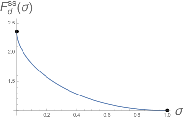
Figure 10: (Color online) Quenched steady-state depletion enhancement factor $F^{ss}_{d}(\sigma)$ above the corresponding ground state value as a function of $\sigma=a_{i}/a_{f}$ following a quench from $a_{i}\to a_{f}$. The two dots coprrespond to the maximum enhancement $F^{ss}_{d}(0)=3\pi/4$ (quenching a non-interacting gas or quenching to unitarity) and minimum enhancement $F^{ss}_{d}(1)=1$ (no quench), respectively.

IV.2 Bragg spectroscopy: structure function

A two-time structure function $S_{\bf q}(t,t^{\prime})=\langle\delta\hat{n}(-{\bf q},t)\delta\hat{n}({\bf q},t^{\prime})\rangle$ is another central probe of the nonequilibrium dynamics of degenerate atomic gases. It can be measured via Bragg spectroscopy through a stimulated two-photon transitions Papp , and via a correlation function of a measured density excitation, $\delta\hat{n}({\bf q},t)$ at momentum ${\bf q}$ and time $t$ ChinGurarie13 . The former thus allowed measurements of the excitation spectrum of a strongly interacting (⁸⁵Rb) BEC, near unitarity ($na^{3}_{s}\gg 1$), demonstrating a large deviation from the Bogoluibov and Lee-Huang-Yang (LHY) prediction of Sec. (II.1). The latter technique was used to characterize dynamics of a Feshbach-resonant Cesium gas, following a shallow quench in its scattering length ChinGurarie13 .

With current experiments in mind, for simplicity we focus on the equal-time $t=t^{\prime}$ structure function (nontrivial for nonequilibrium dynamics),

$$S_{\bf q}(t) = \langle\delta\hat{n}(-{\bf q},t)\delta\hat{n}({\bf q},t)\rangle,$$ (55)

$$= \frac{1}{V}\int_{{\bf r},{\bf r}^{\prime}}e^{i{\bf q}\cdot({\bf r}-{\bf r}^{\prime})}\langle\hat{\psi}^{\dagger}({\bf r},t)\hat{\psi}({\bf r},t)\hat{\psi}^{\dagger}({\bf r}^{\prime},t)\hat{\psi}({\bf r}^{\prime},t)\rangle_{c},$$

$$\approx S^{0}_{\bf q}(t)+\delta S^{B}_{\bf q}(t),$$

where

$$S^{0}_{\bf q}(t) = n_{c}\left[\langle\hat{a}_{\bf q}^{\dagger}(t)\hat{a}_{\bf q}(t)\rangle+\langle\hat{a}_{-{\bf q}}(t)\hat{a}_{-{\bf q}}^{\dagger}(t)\rangle\right.$$

$$\left.+\langle\hat{a}_{-{\bf q}}(t)\hat{a}_{\bf q}(t)\rangle+\langle\hat{a}_{\bf q}^{\dagger}(t)\hat{a}_{-{\bf q}}^{\dagger}(t)\rangle\right],$$

$$= n_{c}\left[C_{q}^{11}(t)+C_{q}^{22}(t)+C_{q}^{21}(t)+C_{q}^{12}(t)\right],$$

and

$$\delta S^{B}_{\bf q}(t) = \frac{1}{V}\sum_{{\bf k}\neq 0}\left[\langle\hat{a}_{\bf k}^{\dagger}(t)\hat{a}_{\bf k}(t)\rangle\langle\hat{a}_{{\bf k}-{\bf q}}(t)\hat{a}_{{\bf k}-{\bf q}}^{\dagger}(t)\rangle\right.$$

$$\left.+\langle\hat{a}_{{\bf k}}^{\dagger}(t)\hat{a}_{-{\bf k}}^{\dagger}(t)\rangle\langle\hat{a}_{{\bf k}-{\bf q}}(t)\hat{a}_{-{\bf k}+{\bf q}}(t)\rangle\right],$$

$$= \frac{1}{V}\sum_{{\bf k}\neq 0}\left[C_{k}^{11}(t)C_{-k+q}^{22}(t)+C_{k}^{(12)}(t)C_{-k+q}^{(21)}(t)\right],$$

are, respectively the quadratic and quartic contribution to $S_{\bf q}(t)$, both computed within the Bogoluibov approximation.

Utilizing the Bogoluibov analysis of the nonequilibrium quenched dynamics from the previous subsection, (Eqs.(43), (LABEL:Revolv), (45), (46), (47)) the leading quadratic contribution to $S^{B}_{\bf q}(t)$ is given by ChinGurarie13

$$S^{0}_{\bf q}(t) = S^{0}_{q}\left[1+\frac{E_{qi}^{2}-E_{qf}^{2}}{E_{qf}^{2}}\sin^{2}(E_{qf}t)\right],$$ (58)

where as a check, at initial time $S_{\bf q}^{0}(t=0)$ and/or for no-quench $g_{i}=g_{f}$ above expression reduces to the pre-quench $t=0^{-}$ structure function,

$$S^{0}_{q} = n\frac{\epsilon_{q}}{E_{qi}}\coth\left({\frac{1}{2}}\beta E_{qi}\right),$$ (59)

at temperature $T=1/\beta$.

In dimensionless units $\hat{q}=q/\sqrt{2mng_{f}}$, $\hat{t}=ng_{f}t$ and $\hat{\beta}=ng_{f}\beta$, it is given by

$$S_{\hat{q}}^{0}(\hat{t})=\frac{\hat{q}\coth(\hat{\beta}\hat{q}\sqrt{\hat{q}^{2}+2\sigma})}{\sqrt{\hat{q}^{2}+2\sigma}}\left[1-\frac{2(1-\sigma)}{\hat{q}^{2}+2}\sin^{2}\left(\hat{t}\hat{q}\sqrt{\hat{q}^{2}+2}\right)\right]\ \ \ \ \ \$$ (60)

and plotted in Fig.(11).

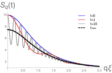
Figure 11: (Color online) Time evolution of the structure function $S_{\bf q}(t)$ defined in the text following a scattering length quench from $0.5a_{f}\to a_{f}$, referring to Eq. (60) using Bogoluibov approximation. It illustrates, following the quench, that the initial ground state structure function (highest curve) develops oscillations and becomes lower, and after some pre-thermalization timescale approaches the steady-state distribution (lowest dashed black curve). Here momentum and time are rescaled by $\xi\equiv 1/\sqrt{2mng_{f}}$ and $t_{0}\equiv 1/(ng_{f})$, respectively. The temperature $T=10ng_{f}$, for a typical ⁸⁵Rb experiment with $n=5\times 10^{12}cm^{-3}$, $a_{f}=1100a_{0}$, corresponds to 16 $nK$.

Utilizing above Bogoluibov analysis, we have further shown that the higher-order correction, $\delta S_{\bf q}^{B}(t)$ in 3d at $T=0$ is given by

$$\delta S_{\bf q}^{B}(0) = \int_{\bf k}\left[u_{ki}v_{ki}u_{-{\bf k}+{\bf q},i}v_{-{\bf k}+{\bf q},i}+u_{ki}^{2}v_{-{\bf k}+{\bf q},i}^{2}\right],$$ (61)

$$= \int_{\bf k}\left[\frac{g_{i}^{2}n^{2}+(\varepsilon_{ki}+E_{ki})(\varepsilon_{-{\bf k}+{\bf q},i}-E_{-{\bf k}+{\bf q},i})}{4E_{ki}E_{-{\bf k}+{\bf q},i}}\right],$$

$$\approx \frac{g_{i}^{2}n^{2}}{2c_{i}^{2}}\int_{\bf k}\left[\frac{1}{k^{2}+\xi_{i}^{2}k^{4}}+O(q)\right],$$

$$\propto n(na_{i}^{3})^{1/2}\left[1+O(q)\right],$$

and for weak interaction ($na^{3}_{s}\ll 1$) it is subdominant to $S_{\bf q}^{0}(t)$. It can, however, become important at finite temperature, lower dimensions and strong interactions.

IV.3 RF spectroscopy

Radio frequency (RF) spectroscopy is another important probe that has been fruitfully utilized to study spectroscopy and dynamics of resonant Fermi JinBCS-BEC and Bose Wild gases. Quite closely related to photoemission spectroscopy of solid state materials, the RF signal is the number of atoms $N_{b}(\omega_{RF})$, that undergoes a hyperfine transition from the many-body state of interest, $E_{a}$ to a weakly interacting state $E_{b}=E_{a}+\omega_{0}$, in response to the stimulated RF pulse at frequency $\omega_{RF}$.

For a weak RF pulse, the governing Hamiltonian

$$\hat{H} = \hat{H}(\hat{a}_{\bf k},\hat{a}^{\dagger}_{\bf k})+\sum_{{\bf k}}(\epsilon_{\bf k}+\omega_{0})\hat{b}_{\bf k}^{\dagger}\hat{b}_{\bf k}+\sum_{{\bf k}}I(t)\hat{b}_{\bf k}^{\dagger}\hat{a}_{\bf k}+h.c.,$$ (62)

$$\equiv \hat{H}_{0}+\hat{H}_{RF}(t),$$

is a sum of the interacting Hamiltonian for the system of $\hat{a}_{\bf k}$ bosons studied in previous subsections, the noninteracting vacuum Hamiltonian for the $\hat{b}_{\bf k}$ bosons, and the RF pulse coupling operator $\hat{H}_{RF}(t)$ that drives the transitions between the two hyperfine states, allowing a conversion of $\hat{a}_{\bf k}$ into $\hat{b}_{\bf k}$.

The RF spectroscopy signal $N_{b}(\omega)$ measures the number of $\hat{b}$ atoms transferred for an RF pulse at frequency $\omega$. It can be evaluated via $N_{b}(\omega)=\int_{0}^{\infty}dt\langle\hat{J}(t)\rangle$, where $\hat{J}(t)$ is the $\hat{a}\rightarrow\hat{b}$ “current” operator

$$\hat{J}(t)\equiv\dot{\hat{N}}_{b} = -i\sum_{\bf k}[\hat{b}_{\bf k}^{\dagger}\hat{b}_{\bf k},\hat{H}],$$ (63)

$$= -i\sum_{\bf k}\left[I(t)\hat{b}_{\bf k}^{\dagger}\hat{a}_{\bf k}-I^{*}(t)\hat{a}_{\bf k}^{\dagger}\hat{b}_{\bf k}\right].\ \ \ \$$

Appropriate for experiments, we focus on a weak RF pulse and calculate the response signal perturbatively in $I(t)$, working in the interaction representation, with $\hat{J}_{I}(t)=e^{i\int_{0}^{t}dt^{\prime}\hat{H}_{0}}\hat{J}e^{-i\int_{0}^{t}dt^{\prime}\hat{H}_{0}}$,

$$\langle\hat{J}(t)\rangle = -i\int_{0}^{t}dt^{\prime}\langle\psi|\left[\hat{J}_{I}(t),\hat{H}_{RF}^{I}(t^{\prime})\right]|\psi\rangle,$$ (65)

$$= \int_{0}^{t}dt^{\prime}\sum_{{\bf k}}I^{*}(t^{\prime})I(t)\langle\alpha_{0}|\hat{a}_{{\bf k}}^{\dagger}(t^{\prime})\hat{a}_{\bf k}(t)|\alpha_{0}\rangle$$

$$\times e^{i(\epsilon_{k}+\omega_{0})(t-t^{\prime})}+c.c..$$

Guided by the experimental protocol Makotyn , above we have taken the initial $t=0^{-}$ state $|\psi\rangle=|\alpha_{0}\rangle|0_{b}\rangle$ to be a product of a vacuum of $\hat{b}$ atoms, $|0_{b}\rangle$ and a SF condensate of $\hat{a}$ atoms, $|\alpha_{0}\rangle$, a vacuum of the Bogoluibov quasi-particles, $\hat{\alpha}_{\bf k}|\alpha_{0}\rangle=0$ for the pre-quench interaction $g_{i}$. The analysis can be straightforwardly generalized to other initial conditions and finite temperature.

It is clear from (65) that the RF signal is not generically proportional to the momentum distribution function $n_{k}(t)=\langle\hat{a}_{{\bf k}}^{\dagger}(t)\hat{a}_{\bf k}(t)\rangle$. The latter requires a sufficiently narrow pulse so as to keep $t\approx t^{\prime}$. Furthermore, a narrow excitation bandwidth is required. Under these conditions indeed we expect that at time $t$ the number of atoms $\hat{b}_{\bf k}$ produced by the RF pulse is proportional to the number of atoms $\hat{a}_{\bf k}$ with momentum ${\bf k}$, such that the resonance condition $E_{kf}-\epsilon_{k}-\omega_{0}=\omega_{RF}$ is satisfied.

Following the experiment Wild , we take the RF pulse to be a real part of

$$I(t)=I_{0}e^{-(t-t_{0})^{2}/\tau^{2}}e^{-i\omega_{RF}t},$$ (66)

with a carrier frequency $\omega_{RF}$ and a Gaussian envelope of width $\tau\gg 1/\omega_{RF}$, ensuring that the excitation is at a well-defined frequency. At the same time, in order to probe the evolving condensate dynamics at a specific time $t$, a short pulse that is narrow on the time scale of the ramp time (that can be made as short as a few microseconds) and on the characteristic many-body time scale (experimentally on the order of few hundred microseconds) that controls the condensate evolution, is required. In JILA experiment Wild , the width $\tau$ ranges from $25\mu s$ to $200\mu s$ with $\omega_{RF}\approx 2\pi\times 50$kHz.

From the analysis of the previous section, the correlator inside Eq. (65) is given by

$$\langle\hat{a}^{\dagger}_{k}(t^{\prime})\hat{a}_{k}(t)\rangle=C_{k}^{11}(t^{\prime},t),\ \ \ \ \ \ \$$

$$= u_{k}^{2}\sinh^{2}\Delta\theta_{k}e^{iE_{kf}(t^{\prime}-t)}+v^{2}_{k}\cosh^{2}\Delta\theta_{k}e^{-iE_{kf}(t^{\prime}-t)}$$

$$+u_{k}v_{k}\cosh\Delta\theta_{k}\sinh\Delta\theta_{k}(e^{iE_{kf}(t^{\prime}+t)}+e^{-iE_{kf}(t^{\prime}+t)}).$$

Using it inside Eq. (65) and leaving the detailed analysis to Appendix D.3, in the limit of $t\gg t_{0}\gg\tau\gg\omega_{RF}^{-1}$ we obtain

$$N_{b}(\omega_{RF}) = 2\pi\tau^{2}I^{2}_{0}\sum_{{\bf k}}\left[e^{-\frac{1}{2}(\epsilon_{k}+\omega_{0}-\omega_{RF}-E_{k})^{2}\tau^{2}}u^{2}_{k}\sinh^{2}\Delta\theta_{k}+e^{-\frac{1}{2}(\epsilon_{k}+\omega_{0}-\omega_{RF}+E_{k})^{2}\tau^{2}}v^{2}_{k}\cosh^{2}\Delta\theta_{k}\right.$$ (68)

$$\left.+u_{k}v_{k}\sinh 2\Delta\theta_{k}e^{-\frac{1}{2}((\epsilon_{k}+\omega_{0}-\omega_{RF})^{2}+E^{2}_{k})\tau^{2}}\cos 2Et_{0}\right].$$

Although the general result is quite involved, it simplies considerably in various important limits. For the case of broad pulse $\tau\omega_{RF}\gg 1$ with a well-defined frequency, the Gaussian factors reduce to energy-conserving $\delta$-functions. In the simplest equilibrium case, where the ground state’s $n_{k}$ ($=v^{2}_{k}$ in the Bogoluibov approximation) is probed, $\Delta\theta_{k}=0$, and we find

$$N^{gs}_{b}(\omega_{RF}) = (2\pi)^{3/2}\tau I^{2}_{0}\sum_{{\bf k}}\delta(\omega_{RF}-\omega_{0}-\epsilon_{k}-E_{k})n_{k}$$

$${}_{\omega_{RF}\gg\omega_{0}} = \frac{\tau I_{0}^{2}V}{\sqrt{2\pi m}}\frac{C_{gs}}{|\omega_{RF}-\omega_{0}|^{3/2}}.$$ (69)

In the last equality we focussed on the large frequency tail probed in the experiments Wild and $C_{gs}$ is Tan’s contact, that in the Bogoluibov approximation is given by $C_{gs}^{B}=16\pi^{2}n^{2}a_{s}^{2}$.

For a measurement of the large frequency tail, $\omega_{RF}\gg\omega_{0}$ following a quench at $t=0$, it is clear from Eq. (68) that only the second term contributes, giving

$$N_{b}(\omega_{RF}) = (2\pi)^{3/2}\tau I^{2}_{0}\sum_{{\bf k}}\delta(\omega_{RF}-\omega_{0}-\epsilon_{k}-E_{k})$$

$$\hskip 71.13188pt\times\ n^{f}_{k}\cosh^{2}\Delta\theta_{k}$$

$${}_{\omega_{RF}\gg\omega_{0}} = \frac{\tau I_{0}^{2}V}{\sqrt{2\pi m}}\frac{C_{f}}{|\omega_{RF}-\omega_{0}|^{3/2}}.$$ (70)

where within Bogoluibov approximation

$$C_{f}=16\pi^{2}n^{2}a_{f}^{2}.$$ (71)

This indicates that, while the overall momentum distribution function $n_{k}(t)$ exhibits nontrivial post-quench dynamics, the large tail of RF spectrum is not affected by the quench dynamics, and provides information about short-scale correlations in the ground state of the final state.

V Finite-rate ramp

Having studied the idealized case of a sudden $g_{i}\rightarrow g_{f}$ quench, we now analyze the dynamics following a more experimentally realistic finite-rate ramp. We model it by an idealized time-dependent coupling

$$g(t) = \left\{\begin{array}[]{ll}g_{i}+(g_{f}-g_{i})t/\tau,&\mbox{for $t<\tau$},\\ g_{f},&\mbox{for $t>\tau$},\end{array}\right.$$ (74)

with ramp time $\tau$, illustrated in Fig. 12.

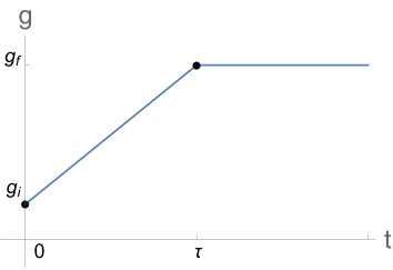
Figure 12: (Color online) Protocol of a linear ramp of coupling strength $g$. Starting with $g=g_{i}$ at ${t}=0$, the coupling strength is ramped to $g=g_{f}$ over ramp time $\tau$.

To this end, we solve the corresponding Heisenberg equations of motion

$$i\begin{pmatrix}\dot{\hat{a}}_{\bf k}\\ -\dot{\hat{a}}^{\dagger}_{-{\bf k}}\end{pmatrix} = \begin{pmatrix}\epsilon_{k}+ng(t)&ng(t)\\ ng(t)&\epsilon_{k}(t)+ng(t)\end{pmatrix}\begin{pmatrix}\hat{a}_{\bf k}(t)\\ \hat{a}^{\dagger}_{-{\bf k}}(t)\end{pmatrix}\;\;\;\;\;\;\;\;\;$$ (75)

by expressing the atomic operators $\hat{a}_{\bf k}(t)$, $\hat{a}^{\dagger}_{\bf k}(t)$ in terms of the Bogoluibov quasi-particles $\hat{\alpha}_{\bf k}$, $\hat{\alpha}^{\dagger}_{\bf k}$ of $\hat{H}(t=0)$ at the start of the ramp

$$\begin{pmatrix}\hat{a}_{\bf k}\\ \hat{a}^{\dagger}_{-{\bf k}}\end{pmatrix}=\begin{pmatrix}u_{k}(t)&v^{*}_{k}(t)\\ v_{k}(t)&u^{*}_{k}(t)\end{pmatrix}\begin{pmatrix}\hat{\alpha}_{\bf k}\\ \hat{\alpha}^{\dagger}_{-{\bf k}}\end{pmatrix}\equiv U_{k}(t)\begin{pmatrix}\hat{\alpha}_{\bf k}\\ \hat{\alpha}^{\dagger}_{-{\bf k}}\end{pmatrix}.\;\;\;$$ (76)

The dynamics is then encoded in the time evolution of a spinor $(u_{k}(t),v_{k}(t))$, with components satisfying

$$i\dot{u}_{\hat{k}} =(\hat{k}^{2}+\hat{g}(t))u_{\hat{k}}+\hat{g}(t)v_{\hat{k}},$$ (77a)

$$-i\dot{v}_{\hat{k}} =(\hat{k}^{2}+\hat{g}(t))v_{\hat{k}}+\hat{g}(t)u_{\hat{k}},$$ (77b)

where $\hat{g}(t)\equiv g(t)/g_{f}$, $\hat{t}\equiv ng_{f}t$ and $\hat{k}^{2}\equiv k^{2}/(2mng_{f})$. In term of above dimensionless variables, Eq. (74) becomes

$$\hat{g}(\hat{t}) = \left\{\begin{array}[]{ll}\sigma+\gamma\hat{t},&\mbox{for $t<\tau$},\\ 1,&\mbox{for $t>\tau$},\end{array}\right.$$ (80)

where we have defined a dimensionless ramp rate $\gamma\equiv(1-\sigma)/(ng_{f}\tau)$. We then solve these numerically, subject to the initial conditions

$$u_{k}(0) = \frac{1}{2^{1/2}}\left(\frac{{\hat{k}}^{2}+\sigma}{\sqrt{{\hat{k}}^{2}({\hat{k}}^{2}+2\sigma)}}+1\right)^{1/2},$$ (81a)

$$v_{k}(0) = -\frac{1}{2^{1/2}}\left(\frac{{\hat{k}}^{2}+\sigma}{\sqrt{{\hat{k}}^{2}({\hat{k}}^{2}+2\sigma)}}-1\right)^{1/2},$$ (81b)

that diagonalize the initial Hamiltonian at $t=0$.

We focus on the momentum distribution at $T=0$

$$n_{k}(t)=\langle 0^{-}|a^{\dagger}_{k}(t)a_{k}(t)|0^{-}\rangle=|v_{k}(t)|^{2},$$ (82)

and condensate fraction

$$n_{c}(t)=1-n_{d}(t)=1-V\int\frac{d^{3}k}{(2\pi)^{3}}n_{k}({t}).$$ (83)

We apply this analysis to interpret experiments by Claussen, et al., Claussen , where dynamics of finite-rate ramp pulse was studied as a function of ramp time $\tau$ and heretofore remained unexplained.

In Fig. 13 we plot the time dependence of the resulting condensate fraction for two densities and fixed ramp rate. Using the parameters reported in Claussen , we obtain results in qualitative agreement with these experimental measurement.

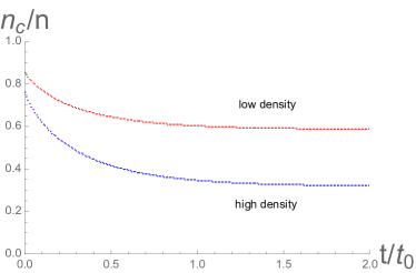
Figure 13: (Color online) Dynamics of the condensate fraction $n_{c}(t)/n$ for high density $n=1.9\times 10^{13}cm^{-3}$ (lower blue curve) and low density $n=0.7\times 10^{13}cm^{-3}$ (upper red curve), after a linear interaction ramp $g(t)$ from $g_{i}=0.001g_{f}$ to $g_{f}$ with dimensionless ramp rate $\hat{\gamma}\equiv(1-\sigma)/(\tau ng_{f})=5$. Following the experiments in Ref.Claussen, the final scattering length is $a_{f}=2700a_{0}$ and the corresponding pre-thermalization timescale $t_{0}=150\mu s$.

To explore the ramp rate dependence of the dynamics as studied by Claussen, et al., Claussen , in Fig. 14 we plot the condensate fraction as a function of ramp time $\tau$ (inverse ramp rate, in units of $(1-\sigma)/(ng_{f})$). As illustrated there, we find that the dependence on the ramp time $\tau$ is nonmonotonic and is a function of the hold time $t$. This can be understood by noting that for a sudden quench (vanishing $\tau$) at long hold times, the condensate is depleted more strongly than the ground state depletion for $g_{f}$. On the other hand, at short hold times the quenched depletion is given by the ground state for $g_{i}$. In contrast, for a slow adiabatic ramp (large $\tau$) the condensate fraction asymptotes to the adiabatic limit corresponding to that of a ground state for $g_{f}$.

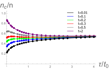
Figure 14: (Color online) Dependence of condensate fraction $n_{c}/n$ on the ramp duration $\tau$ for various hold time $t$ in units of pre-thermalization timescale $t_{0}=\hbar/(ng_{f})$ (From lowest curve to highest one, the hold times are $\hat{t}=0.01,0.1,0.2,0.3,0.5,2$, respectively). Following the experiments in Ref. Claussen, we take the final scattering length to be $a_{f}=2700a_{0}$ with $a_{i}=0.001a_{f}$ and $n=1.9*10^{12}cm^{-3}$.

Thus, for short hold time the condensate fraction decreases from $n_{c}^{g_{i}}$ to $n_{c}^{g_{f}}$ with increasing $\tau$. For long hold times, the condensate fraction increases from pre-thermalized value $n_{c}^{ss}$ to $n_{c}^{g_{f}}$ with increasing $\tau$. This behavior is qualitatively quite similar to that found in experiments of Ref. Claussen .

VI Dynamics for deep quench

In the present and subsequent sections we study the nonperturbative dynamics following a deep quench, $na^{3}_{f}\gg 1$, a regime of JILA recent experiment Makotyn that is our main focus YinLR14 . In contrast to the well-controlled, perturbative dynamics of a shallow quench discussed in Sec. IV, for deep quenches the condensate depletion dynamics is significant and cannot be neglected.

From the outset, we acknowledge that no rigorous solution in such a nonperturbative regime is available even for a purely repulsive Bose gas ground state. Nevertheless, to make progress we treat this strongly interacting nonequilibrium dynamics utilizing a nonperturbative but uncontrolled self-consistent Bogoluibov treatment. This is analogous to a BCS dynamic mean-field theory Barankov ; AGR06 , with the condensate fraction $n_{c}(t)$ playing the role of the time-dependent order parameter. We thus reduce the problem to a solution of the Bogoluibov dynamics with a time-dependent condensate fraction that is self-consistently determined. This is a dynamical generalization of our analysis of the strongly interacting Bose gas ground state in Sec. III.

Another challenge of this system is the resonant nature of the Bose gas interaction. To handle this we employ a second beyond-Bogoluibov approximation by replacing the scattering length $a_{f}$ by the density dependent scattering amplitude $|f(k_{n},a_{f})|=a_{f}/\sqrt{1+k_{n}^{2}a_{f}^{2}}\equiv\tilde{a}_{f}$, and the Hartree interaction energy $g_{f}n$ by $\tilde{g}_{f}n\equiv\frac{8\pi\epsilon_{F}}{\sqrt{1/(k_{n}a_{f})^{2}+1}}$. This qualitatively captures the crossover from the two-atom regime, $a_{f}\ll n^{-1/3}$ to a finite density limit, when $a_{f}$ reaches inter-particle spacing and the scattering amplitude saturates at $\sim k_{n}^{-1}$. While the detailed nature of this crossover is ad hoc, our qualitative predictions are insensitive to these details and only depend on the limiting values of the two regimes.

Motivated by the experiments Makotyn , we focus on an initial state that is a well-established condensate. This allows us to make progress in treating the resonant interactions by expanding in finite-momentum quasi-particle fluctuations about a macroscopically occupied ${\bf k}=0$ state. Following a sudden quench, $g_{i}\rightarrow g_{f}$, we approximate the Hamiltonian by a quadratic time-dependent form,

$$\hat{H}_{f}(t) = {\frac{1}{2}}\sum_{{\bf k}\neq 0}\begin{pmatrix}\hat{a}_{\bf k}^{\dagger}&\hat{a}_{-{\bf k}}\\ \end{pmatrix}\begin{pmatrix}\epsilon_{k}+g_{f}n_{c}(t)&g_{f}n_{c}(t)\\ g_{f}n_{c}(t)&\epsilon_{k}+g_{f}n_{c}(t)\\ \end{pmatrix}\begin{pmatrix}\hat{a}_{\bf k}\\ \hat{a}_{-{\bf k}}^{\dagger}\\ \end{pmatrix}$$ (84)

$$\equiv {\frac{1}{2}}\sum_{{\bf k}\neq 0}\hat{\Phi}^{\dagger}_{\bf k}(t)\cdot\hat{h}_{kf}(t)\cdot\hat{\Phi}_{\bf k}(t).$$

The key new ingredient (in contrast to Bogoluibov theory of Sec. II.1) is the nontrivial time-dependent condensate density, that is self-consistently determined by the total atom conservation,

$$n_{c}(t)=n-\frac{1}{V}\sum_{{\bf k}\neq 0}\langle 0^{-}|\hat{a}_{\bf k}^{\dagger}(t)\hat{a}_{\bf k}(t)|0^{-}\rangle,$$ (85)

evaluated in the pre-quench state $|0^{-}\rangle$ at $t=0^{-}$. In a homogeneous case, this is equivalent to a solution of the Gross-Petaevskii equation for the condensate order parameter $\Psi_{0}$, coupled to the Heisenberg equation of motion for the finite momentum quasi-particles. Focussing on zero temperature, we take the initial state $|0^{-}\rangle$ to be the vacuum with respect to the quasi-particles $\hat{\alpha}_{\bf k}$, that diagonalize the initial Hamiltonian, $\hat{H}_{i}=\sum_{\bf k}E_{ki}\hat{\alpha}_{\bf k}^{\dagger}\hat{\alpha}_{\bf k}$, characterized by a pre-quench $t=0^{-}$ scattering length, $a_{i}$.

The corresponding Heisenberg equation of motion

$$i\sigma_{z}\partial_{t}\hat{\Phi}_{\bf k}(t)=\hat{h}_{kf}(t)\cdot\hat{\Phi}_{\bf k}(t)$$ (86)

for $\hat{\Phi}_{\bf k}(t)=(\hat{a}_{\bf k}(t),\hat{a}_{-{\bf k}}^{\dagger}(t))$ is conveniently encoded in terms of a time-dependent Bogoluibov transformation $U_{kf}(t)$,

$$\hat{\Phi}_{\bf k}(t)=U_{{\bf k}f}(t)\hat{\Psi}_{\bf k},$$ (87)

where

$$U_{kf}(t) = \begin{pmatrix}u_{kf}(t)&v^{*}_{kf}(t)\\ v_{kf}(t)&u^{*}_{kf}(t)\end{pmatrix}$$ (88)

and $\hat{\Psi}_{\bf k}=(\hat{\beta}_{\bf k},\hat{\beta}^{\dagger}_{-{\bf k}})$ are time-independent bosonic reference operators, that diagonalize the Hamiltonian at the initial time $t=0^{+}$ after the quench, with $\hat{H}_{f}(0^{+})=\sum_{\bf k}E_{kf}(0^{+})\hat{\beta}_{\bf k}^{\dagger}\hat{\beta}_{\bf k}$.

Equivalently, $U^{\dagger}_{kf}(0^{+})h_{kf}(0^{+})U_{kf}(0^{+})=E_{kf}(0^{+})=\sqrt{\epsilon_{k}^{2}+2g_{f}n_{c}(0^{+})\epsilon_{k}}$, fixing the initial condition

$$u_{kf}(0^{+}) = \sqrt{{\frac{1}{2}}\left(\frac{\epsilon_{k}+g_{f}n_{c}(0^{+})}{E_{f}(0^{+})}+1\right)},$$ (89a)

$$v_{kf}(0^{+}) = -\sqrt{{\frac{1}{2}}\left(\frac{\epsilon_{k}+g_{f}n_{c}(0^{+})}{E_{f}(0^{+})}-1\right)},$$ (89b)

for spinor $\psi_{kf}(t)\equiv(u_{kf}(t),v_{kf}(t))$, that evolves according to

$$i\sigma_{z}\partial_{t}{\psi}_{kf}(t)=\hat{h}_{kf}(t)\cdot{\psi}_{kf}(t).$$ (90)

As for the Bogoluibov analysis in Sec. II.1, because the initial state $|0^{-}\rangle$ is a vacuum of $\hat{\alpha}_{k}$, it is convenient to further express $\hat{\Phi}_{\bf k}(t)=(\hat{a}_{\bf k}(t),\hat{a}_{-{\bf k}}^{\dagger}(t))$ in terms of the pre-quench quasi-particle basis $\hat{\Psi}_{{\bf k}}(0^{-})=(\hat{\alpha}_{\bf k},\hat{\alpha}^{\dagger}_{\bf k})$,

$$\hat{\Phi}_{\bf k}(t) = U_{kf}(t)U_{kf}^{-1}(0^{+})U_{ki}(0^{-})\hat{\Psi}_{{\bf k}}(0^{-}),$$ (91a)

$$\equiv U_{k}(t)\hat{\Psi}_{{\bf k}}(0^{-}).$$ (91b)

The post-quench dynamics is thus fully determined by the self-consistent solutions $\psi_{kf}(t)$ of Eq. (90), together with the atom number conservation constraint, (85). This can be obtained numerically in essentially exact way, as we will demonstrate in Sec. VI.2.

VI.1 Quasi-adiabatic self-consistent approximation

Despite availability of the numerical solution, to gain further physical insight it is of interest to obtain an approximate analytical solution. To this end we note that for a given slowly evolving condensate density satisfying ${\dot{n}_{c}(t)}/{n}\ll{E^{3}_{kf}}/(\hbar ng\epsilon_{k})=(\epsilon_{k})^{1/2}(\epsilon_{k}+2gn_{c})^{3/2}/(\hbar ng)$ (see Eq. (172) and YinLR14 ; KainLing ), Eq. (90) can be well-approximated by an instantaneous, quasi-adiabatic Bogoluibov transformation of $\hat{H}_{f}(t)$ (see Appendix B),

$$U_{kf}(t)=\begin{pmatrix}u_{k}(t)e^{-i\int_{0}^{t}E_{kf}(t^{\prime})}&v_{k}(t)e^{i\int_{0}^{t}E_{kf}(t^{\prime})}\\ v_{k}(t)e^{-i\int_{0}^{t}E_{kf}(t^{\prime})}&u_{k}(t)e^{i\int_{0}^{t}E_{kf}(t^{\prime})}\\ \end{pmatrix}.\quad$$ (92)

In above, $(u_{k}(t),v_{k}(t))$ is the instantaneous eigenstate of the single-particle Hamiltonian $\hat{h}_{kf}(t)$, with time dependence entering only through the time dependent condensate density, $n_{c}(t)$. Such approximation is in the spirit of the WKB quasi-local treatment of a smoothly varying potential Shankar .

More specifically the solution is given by

$$\begin{split}u_{k}(t)&=\sqrt{\frac{1}{2}\left(\frac{\epsilon_{k}+g_{f}n_{c}(t)}{E_{kf}(t)}+1\right)},\\ v_{k}(t)&=-\sqrt{\frac{1}{2}\left(\frac{\epsilon_{k}+g_{f}n_{c}(t)}{E_{kf}(t)}-1\right)},\\ E_{kf}(t)&=\sqrt{\epsilon_{k}(\epsilon_{k}+2g_{f}n_{c}(t))},\end{split}$$ (93)

with initial condition given by (89a)(89b).

After a tedious but conceptually straightforward calculation that utilizes above relations, we obtain the momentum distribution function

$$\begin{split}n_{k}(t)&=\langle 0^{-}|\hat{a}^{\dagger}_{\bf k}(t)\hat{a}_{\bf k}(t)|0^{-}\rangle\\ &=\frac{\epsilon^{2}_{k}+\epsilon_{k}(g_{i}n+g_{f}n+g_{f}n_{c}(t))+2g_{f}g_{i}n_{c}(t)n+2g_{f}n_{c}(t)n(g_{f}-g_{i})\sin^{2}(\int_{0}^{t}\sqrt{\epsilon_{k}(\epsilon_{k}+2g_{f}n_{c}(t^{\prime}))}dt^{\prime})}{2\sqrt{\epsilon_{k}(\epsilon_{k}+2g_{f}n_{c}(t))}\sqrt{(\epsilon_{k}+2g_{i}n)}\sqrt{(\epsilon_{k}+2g_{f}n)}}-\frac{1}{2},\\ \end{split}$$ (94)

with the condensate density $n_{c}(t)$ self-consistently determined according to $n_{c}(t)=n-\sum_{\bm{k}\neq 0}n_{k}(t)$.

By construction, the above expression for $n_{k}(t=0)$ reduces to the pre-quench momentum distribution function

$$n_{k}(t=0)=\frac{1}{2}\left[\frac{\epsilon_{k}+g_{i}n_{c}(0)}{E_{ki}}-1\right]=n_{ki},$$ (95)

as required by continuity. Furthermore for $g_{f}=g_{i}$, i.e., in the absence of a quench, the time-dependent part of $n_{k}$ drops out and again reduces to $n_{ki}$.

Using (94) the self-consistency condition reduces to a dimensionless form

$$\begin{split}1-\hat{n}_{c}=n^{0}_{d}F_{d}(\hat{n}_{c},\sigma),\end{split}$$ (96)

where $n^{0}_{d}=8/(3\sqrt{\pi})({na_{f}^{3}})^{1/2}$ is the depletion corresponding to the ground state of quenched Hamiltonian, $q\equiv\sqrt{k^{2}/{(2mng_{f})}}$ and $\hat{n}_{c}(t)\equiv n_{c}(t)/n$ are dimensionless variables, and

$$\begin{split}F(\hat{n}_{c},\sigma,t)=3\sqrt{2}\int dqq^{2}\left[\frac{(q^{4}+{q}^{2}(\sigma+1+\hat{n}_{c})+2\sigma\hat{n}_{c}+2\hat{n}_{c}(1-\sigma)\sin^{2}(\int_{0}^{t}ngt\sqrt{q^{2}(q^{2}+2\hat{n}_{c})}))}{2\sqrt{{q}^{2}({q}^{2}+2\hat{n}_{c})}\sqrt{({q}^{2}+2\sigma)}\sqrt{({q}^{2}+2)}}-\frac{1}{2}\right],\end{split}$$ (97)

is the quench-induced depletion-enhancement factor.

We solve Eqs.(96),(97) numerically and plot the depletion fraction $\hat{n}_{d}(t)=1-\hat{n}_{c}(t)$ as a function of time in Fig. 15.

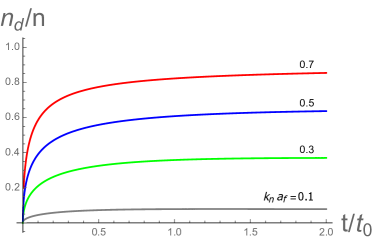
Figure 15: (Color online) Time evolution of the condensate depletion fraction $n_{d}(t)/n$ (treated within a quasi-adiabatic self-consistent dynamic field analysis, referring to Eq. (96)), following a scattering length quench from $k_{n}a_{i}=0.01$ to various $k_{n}a_{f}$ in a resonant Bose gas. Here we normalize the time with the pre-thermalization timescale $t_{0}=1/ng_{f}=m/(4\pi a_{f}n)$ associated with $k_{n}a_{f}=1$ (where $k_{n}\equiv n^{1/3}$).

We observe that the depletion fraction increases smoothly with time on the scale $t_{0}=m/(4\pi a_{f}n)$, reaching a stationary steady-state $n_{d}^{ss}$, that is an increasing function of the quench depth $k_{n}a_{f}$. Even for a deep quench to a unitary point, the self-consistent treatment ensures that the depletion, always remains below the total atom density. The slow time dependence of $n_{d}(t)$ justifies the quasi-static approximation for the high momenta ($k\gtrsim 1/\xi$) quasi-particles, but fails for the low-momenta ($k\lesssim 1/\xi$) Goldstone modes. We further note that the asymptotic depletion $n_{d}^{ss}$ always significantly exceeds the depletion for the ground state corresponding to the quenched scattering length $a_{f}$. Thus not surprisingly the thermal equilibrium is never reached in our effectively integrable harmonic model.

Having computed the condensate depletion and the associated condensate density, $n_{c}(t)$, Eq. (94) immediately gives us the momentum distribution function $n_{k}(t)$, that we illustrate in Fig. 16.

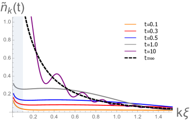
Figure 16: (Color online) Time evolution of the (column-density) momentum distribution function, $\tilde{n}_{{\bf k}_{\perp}}(t)\equiv\int dk_{z}n_{\bf k}(t)$ following a scattering length quench $k_{n}a_{i}=0.01\rightarrow k_{n}a_{f}=0.5$ (where $k_{n}\equiv n^{1/3}$) in a resonant Bose gas, computed with quasi-adiabatic self-consistent approximation. Here we normalize the time with the pre-thermalization timescale $t_{0}=1/ng_{f}=m/(4\pi a_{f}n)$ associated with $k_{n}a_{f}=1$. Here momentum and time are rescaled with $\xi\equiv 1/\sqrt{2mng_{f}}$ and $t_{0}\equiv 1/(ng_{f})$, respectively. The grey region indicates a range of momenta not resolved in JILA experiments, due to initial inhomogeneous real space density profile and finite trap size.

Following a quench, the initially narrow (for $g_{i}\ll g_{f}$) momentum distribution function (corresponding to pre-quench BEC state) displays rich dynamics. Within 2-body interaction scale it quickly develops a large momentum tail corresponding to the strong atom-atom interaction $g_{f}$. With time, the suddenly turned on interaction promotes an increasing number of atom pairs from the condensate to finite momentum excitations. The momentum distribution tail fills in from high to low momenta as pair-excitation dynamics at momentum $k$ dephases with frequency $2E_{kf}$. Thus, at time $t$, $n_{k}(t)$ establishes a pre-thermalized power-law steady-state for momenta $k>k_{pth}(t)$, latter set by $E_{k_{pth},f}t\approx 1$. Equivalently, it takes time

$$t_{pth} \approx \frac{1}{E_{k_{pth},f}},$$ (98a)

$$\sim \left\{\begin{array}[]{ll}1/k^{2},&\mbox{for $k\gg 1/\xi$},\\ 1/k,&\mbox{for $k\ll 1/\xi$},\end{array}\right.$$ (98d)

for the pre-thermalization to reach a stationary state down to momentum $k$, a distinctive feature that is consistent with JILA experiments Makotyn .

As illustrated in Fig. 17, in the long time limit (around $170\mu$-sec in ⁸⁵Rb experiments Makotyn ) a quenched Bose gas approaches a pre-thermalized stationary state, as reflected by a time-independent power-law momentum distribution

$$n_{k}(t) = \frac{\hat{k}^{4}+\hat{k}^{2}(\sigma+1+\hat{n}^{ss}_{c})+\hat{n}^{ss}_{c}(1+\sigma)}{2\sqrt{\hat{k}^{2}(\hat{k}^{2}+2\hat{n}^{ss}_{c})}\sqrt{(\hat{k}^{2}+2\sigma)}\sqrt{(\hat{k}^{2}+2)}}-\frac{1}{2},$$ (99)

$$\sim C^{ss}/k^{4},\qquad\mbox{for $k\xi\gg 1$},$$

where $C^{ss}=(4\pi a_{f}n)^{2}\left[n^{ss}_{c}/{n}+(1-\sigma)^{2}\right]$ is the nonequilibrium analog of Tan’s contact Tan . Within the above self-consistent Bogoluibov approximation the quasi-particles do not scatter, precluding full thermalization. The resulting final state remains nonequilibrium, completely determined by the depth-quench parameter $\sigma$, characterized by a diagonal density matrix ensemble.

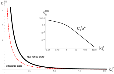
Figure 17: (Color online) A long-time nonequilibrium steady-state momentum distribution function $n_{k}^{ss}$ of a resonant Bose gas following a scattering length quench $k_{n}a_{i}=0.01\rightarrow k_{n}a_{f}=0.5$ (solid black curve), as compared to ground state momentum distribution at $k_{n}a_{f}$ (red dashed curve). The inset illustrates the emergence of a $1/k^{4}$ large momentum tail, corresponding to a steady-state “contact”.

With the above solution of the self-consistent post-quench dynamics, we can now also calculate other physical observables, such as, for example the structure function measured in Bragg spectroscopy. Using above analysis for $S_{\bf q}(t)$ in Eq. (55) we find

$$\begin{split}S_{\hat{q}}(t)&=\coth(\hat{\beta}\hat{q}\sqrt{\hat{q}^{2}+2\sigma})\frac{\hat{q}}{\sqrt{\hat{q}^{2}+2\sigma}}\\ &\quad\times\bigg{(}\frac{\sqrt{\hat{q}^{2}+2}}{\sqrt{\hat{q}^{2}+2\hat{n}_{c}(t)}}\\ &\qquad-\frac{2(1-\sigma)\sin^{2}(\hat{q}t\sqrt{\hat{q}^{2}+2\hat{n}_{c}(t)})}{\sqrt{\hat{q}^{2}+2}\sqrt{\hat{q}^{2}+2\hat{n}_{c}(t)}}\bigg{)},\end{split}$$ (100)

where $\hat{q}=q/\sqrt{2mng_{f}}$, $\hat{t}=ng_{f}t$ and $\hat{\beta}=ng_{f}\beta$.

The results are then illustrated in Fig. 5 and 18.

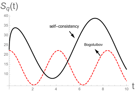
Figure 18: (Color online) Oscillation of structure function $S_{\bf q}(t)$ (treated within a quasi-adiabatic self-consistent dynamic field analysis, thick black curve, referring to Eq. (100)) as a function of time, following a scattering length quench from $0.1a_{f}\to a_{f}$ with $k_{n}a_{f}=0.7$ (where $k_{n}\equiv n^{1/3}$) at momentum $k\xi=0.5$, as compared to Bogoluibov approximation (dashed red curve).

The role of self-consistency is clear: in Fig. 5, as compared with Fig. 11, self-consistency exchanges the relative position of initial and final asymptotic steady-state curve; while in Fig. 18 it shifts the phase as well as modifies the frequency of the structure function oscillation. We expect these features to be experimentally testable by going to a deep quench regimes, $k_{n}a_{f}\gg 1$.

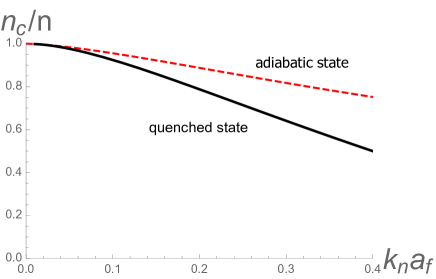
Figure 19: (Color online) Quenched steady state condensate fraction $n_{c}/n$ as a function of $k_{n}a_{f}$ (solid black curve, treated with quasi-adiabatic self-consistent dynamic field, referring to Eq.(96)), as compared with the ground state condensate fraction at $k_{n}a_{f}$ (dashed red curve), both calculated with self-consistency on $n_{c}$.

We emphasize that above analysis utilizes a quasi-adiabatic approximation, valid for ${\dot{n}_{c}(t)}/{n}\ll{E^{3}_{kf}}/(\hbar ng\epsilon_{k})$. As mentioned above we expect it to break down for sufficiently small momenta for slow Goldstone modes as well as large $k_{n}a_{f}$ value, where $\dot{n}_{c}(t)/n$ is large.

VI.2 Exact numerical solution to post quench dynamics

In this subsection we test the validity of above quasi-adiabatic approximation by analyzing the post-quench dynamics through an essentially exact numerical solution of the Heisenberg equation of motion (90). Consistent with our expectations we find that while the former provides an accurate description for a shallow quench and high momenta, it fails quantitatively (though not qualitatively) for $k_{n}a_{f}\gg 1$ and low momenta, $k\ll 1/\xi$.

As derived in previous subsection, the dynamics is governed by Eq. (90) for $\psi_{\bf k}(t)=(u_{kf}(t),v_{kf}(t))$, that relate atomic excitations, $\hat{a}_{\bf k}$ to Bogoluibov quasi-particles $\hat{\beta}_{\bf k}$. Here we solve Eq. (90) numerically together with the number conservation condition on the condensate fraction. In dimensionless form, the equations of motion are given by

$$\begin{split}i\dot{u}_{k}&=(\hat{k}^{2}+\bar{n}(t))u_{k}+\bar{n}(t)v_{k},\\ -i\dot{v}_{k}&=(\hat{k}^{2}+\bar{n}(t))v_{k}+\bar{n}(t)u_{k},\\ \end{split}$$ (101)

with the initial conditions fixed by a requirement that at $t=0$, $\psi(0^{+})$ diagonalizes $\hat{H}_{f}(0^{+})$,

$$u_{k}(t=0) = \sqrt{\frac{1}{2}[E^{-1}_{kf}\left(\epsilon_{k}+n_{c}(0)g_{f}\right)+1]},$$ (102a)

$$= \sqrt{\frac{1}{2}\left(\frac{\hat{k}^{2}+1}{\sqrt{\hat{k}^{2}(\hat{k}^{2}+2)}}+1\right)},$$

$$v_{k}(t=0) = -\sqrt{\frac{1}{2}[E^{-1}_{kf}\left(\epsilon_{k}+n_{c}(0)g_{f}\right)-1]},$$ (102b)

$$= -\sqrt{\frac{1}{2}\left(\frac{\hat{k}^{2}+1}{\sqrt{\hat{k}^{2}(\hat{k}^{2}+2)}}-1\right)},$$

where $\hat{t}\equiv ng_{f}t$, $\hat{k}^{2}\equiv k^{2}/(2mng_{f})$ and $\bar{n}(t)\equiv n_{c}(t)/n$.

Decoupling the $u_{k}(t)$ and $v_{k}(t)$ components

$$\begin{split}\ddot{u}&=[-k^{2}(k^{2}+2\bar{n}(t))+i\frac{\dot{\bar{n}}(t)}{\bar{n}(t)}(k^{2})]u+\frac{\dot{\bar{n}}(t)}{\bar{n}(t)}\dot{u},\\ \ddot{v}&=[-k^{2}(k^{2}+2\bar{n}(t))-i\frac{\dot{\bar{n}}(t)}{\bar{n}(t)}(k^{2})]v+\frac{\dot{\bar{n}}(t)}{\bar{n}(t)}\dot{v},\end{split}$$ (103)

more clearly reveals the relation of these exact equations to the quasi-adiabatic approximation of previous subsection. Indeed the latter is obtained by neglecting $\dot{\bar{n}}(t)/{\bar{n}(t)}$ relative to the instantaneous Bogoluibov dispersion $E_{kf}(t)$, clearly only possible for sufficiently large momenta.

To fully account for the self-consistent dynamics of $n_{c}(t)$, here we solve iteratively the full set of equations (103) (or equivalently Eqs.(101), (102a)(102b)) and (105). With this solution in hand we can compute an arbitrary physical quantity.

Focussing on experimentally accessible momentum distribution, we compute

$$\begin{split}n_{k}(t)&=\langle 0^{-}|\hat{a}^{\dagger}_{\bf k}(t)\hat{a}_{\bf k}(t)|0^{-}\rangle\\ &=|(u_{k}(t)\sinh\Delta\theta_{k}-v^{*}_{k}(t)\cosh\Delta\theta_{k})|^{2},\end{split}$$ (104)

together with the atom number self-consistency condition

$$\begin{split}\bar{n}(t)&=1-\frac{8}{\sqrt{\pi}}(2na^{3}_{f})^{1/2}\int d\hat{k}{\hat{k}}^{2}|(u_{k}(t)\sinh\Delta\theta_{k}\\ &\quad-v^{*}_{k}(t)\cosh\Delta\theta_{k})|^{2}.\end{split}$$ (105)

We illustrate the results in Figs. 1,3, from which we observe that the numerically computed $n_{k}(t)$ and $n_{d}(t)$ quite closely qualitatively resemble the approximate quasi-adiabatic counterparts. Yet, they differ quantitively, particularly in the case of deep quench and for small momenta. The asymptotic time-averaged value of $n_{d}(t)$ always considerably exceeds the corresponding ground state depletion and thus the pre-thermalized system remains out of equilibrium.

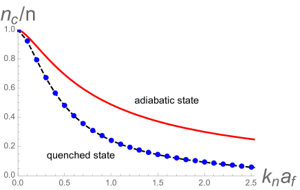
Figure 20: (Color online) Quenched steady-state condensate fraction (dash-dotted blue curve) as a function of $k_{n}a_{f}$, following a quench from $k_{n}a_{i}=0.01\to k_{n}a_{f}$ (where $k_{n}\equiv n^{1/3}$), as compared to the ground state condensate fraction at $k_{n}a_{f}$ (solid red curve, same as in Fig. 2), both calculated within self-consistent dynamic field approximation.

In Fig. 21 we compare the numerical solution with corresponding quantities obtained via various approximate approaches of previous sections. We find that for $k_{n}a_{f}\ll 1$, both the quasi-adiabatic self-consistent solution and numerical self-consistent solution, reduce to that of a straight Bogoluibov approximation, but deviate with increasing depth of the quench, $k_{n}a_{f}$. We observe that in contrast to the adiabatic approximation, the full numerical solution predicts that the condensate fraction remains finite for arbitrary large $k_{n}a_{f}$, arguing that our earlier conjecture of a nonequilibrium phase transition to a “normal” state is likely incorrect YinLR14 .

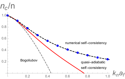
Figure 21: (Color online) Comparison of results from three different approaches to computation of the post-quench steady state condensate fraction $n_{c}/n$: numerical self-consistency (dash-dotted blue), quasi-adiabatic self-consistency (solid red) and Bogoluibov (dashed grey).

VI.3 Generalized Gibbs Ensemble

In the analysis above we found that following a scattering length quench a nonequilibrium state, characterized by a stationary momentum distribution function of atoms emerges in the long time limit. It is thus natural to explore whether this state can be captured by a Generalized Gibbs Ensemble (GGE) Rigola ; RigolOlshanniNaturePRL07 .

At the simplest level of harmonic Bogoluibov description, the final stationary state is completely determined by the initial post-quench momentum distribution function of the quasi-particles $\hat{\beta}_{k}$. The latter is in turn specified by the initial, $a_{i}$ and final $a_{f}$ scattering lengths, i.e., by the initial ground state $|0^{-}\rangle$ (vacuum of $\hat{\alpha}_{k}$) and the post-quench Hamiltonian $\hat{H}(0^{+})$, through the relation (39) derived in Sec. IV.

Since at this harmonic level the energy eigenvalues $E_{kf}$ for each momentum are separately conserved, the distribution of $\hat{\beta}_{\bf k}$ occupations can clearly be captured with GGE

$$\begin{split}\hat{\rho}_{GGE}=Z^{-1}_{GGE}e^{-\sum_{\bf k}\lambda_{k}E_{kf}\hat{\beta}^{\dagger}_{\bf k}\hat{\beta}_{\bf k}},\end{split}$$ (106)

where $Z_{GGE}=Tr\left[e^{-\sum_{\bf k}\lambda_{\bf k}E_{kf}\hat{\beta}^{\dagger}_{\bf k}\hat{\beta}_{\bf k}}\right]$ and $\lambda_{k}$ are the Lagrange multipliers (inverse of effective temperatures) for each conserved mode ${\bf k}$. These are fixed by requiring

$$n_{k}^{\beta} \equiv \langle 0^{-}|\hat{\beta}^{\dagger}_{\bf k}\hat{\beta}_{\bf k}|0^{-}\rangle=\langle\hat{\beta}^{\dagger}_{\bf k}\hat{\beta}_{\bf k}\rangle_{GGE}\equiv Tr(\hat{\beta}^{\dagger}_{\bf k}\hat{\beta}_{\bf k}\hat{\rho}_{GGE}).$$

The analysis from Sec. IV gives the left hand side

$$n_{k}^{\beta}=\frac{1}{4}\left(\frac{E_{kf}}{E_{ki}}+\frac{E_{ki}}{E_{kf}}\right)-{\frac{1}{2}},$$ (108)

determing

$$\lambda_{k}=\frac{1}{E_{kf}}\ln\left(\frac{n_{k}^{\beta}+1}{n_{k}^{\beta}}\right).$$ (109)

We now want to see if the long-time atomic momentum distribution function $n_{k}(t\rightarrow\infty)$ can be characterized by the GGE.

VI.3.1 shallow quench

For a shallow quench, captured by purely harmonic Bogoluibov approximation we have

$$\begin{split}n_{k}(t)&=\langle 0^{-}|\hat{a}^{\dagger}_{\bf k}(t)\hat{a}_{\bf k}(t)|0^{-}\rangle,\\ &=v^{2}_{k}+(u^{2}_{k}+v^{2}_{k})\langle\hat{\beta}^{\dagger}_{\bf k}(t)\hat{\beta}_{\bf k}(t)\rangle\\ &\quad-u_{k}v_{k}\langle\hat{\beta}_{\bf k}(t)\hat{\beta}_{-{\bf k}}(t)+\hat{\beta}^{\dagger}_{\bf k}(t)\hat{\beta}^{\dagger}_{-{\bf k}}(t)\rangle.\end{split}$$ (110)

In the long time limit, the time-dependence of the off-diagonal last terms dephases away, and only first two terms survive. The steady-state momentum distribution $n^{ss}_{k}$ then becomes

$$\begin{split}n^{ss}_{k}=v^{2}_{k}+(u^{2}_{k}+v^{2}_{k})\langle\hat{\beta}^{\dagger}_{\bf k}\hat{\beta}_{\bf k}\rangle\end{split}$$ (111)

Since $\langle\hat{\beta}^{\dagger}_{\bf k}\hat{\beta}_{\bf k}\rangle=\langle\hat{\beta}^{\dagger}_{\bf k}\hat{\beta}_{\bf k}\rangle_{GGE}$, it is clear that in this purely harmonic approximation the GGE does describe the steady-state distribuition.

VI.3.2 deep quench

As we demonstrated in previous subsections, for a deep quench, a self-consistency of condensate density must be implemented. This results to an effective time dependent Hamiltonian. In the simplest quasi-adiabatic approximation, we find

$$\begin{split}n_{k}(t)&=v^{2}_{k}(t)+(u^{2}_{k}(t)+v^{2}_{k}(t))\langle\hat{\beta}^{\dagger}_{\bf k}\hat{\beta}_{\bf k}\rangle\\ &\quad-u_{k}(t)v_{k}(t)\langle\hat{\beta}_{\bf k}(t)\hat{\beta}_{-{\bf k}}(t)+\hat{\beta}^{\dagger}_{\bf k}(t)\hat{\beta}^{\dagger}_{-{\bf k}}(t)\rangle.\end{split}$$ (112)

This leads to a steady-state distribution

$$\begin{split}n^{ss}_{k}=(v^{ss}_{k})^{2}+((u^{ss}_{k})^{2}+(v^{ss}_{k})^{2})\langle\hat{\beta}^{\dagger}_{\bf k}\hat{\beta}_{\bf k}\rangle,\end{split}$$ (113)

where

$$u^{ss}_{k} =\sqrt{\frac{1}{2}\big{(}\frac{\epsilon_{k}+n^{ss}_{c}g_{f}}{E_{kf}}+1\big{)}},$$ (114a)

$$v^{ss}_{k} =-\sqrt{\frac{1}{2}\big{(}\frac{\epsilon_{k}+n^{ss}_{c}g_{f}}{E_{kf}}-1\big{)}},$$ (114b)

$$E_{kf} =\sqrt{{\epsilon_{k}}^{2}+2n^{ss}_{c}g_{f}\epsilon_{k}},$$ (114c)

and $n^{ss}_{c}$ the steady-state condensate density determined by the self-consistency condition. The latter spoils the GGE description of the long-time distribution even in this approximation.

Indeed beyond the quasi-adiabatic approximation the inability of GGE to capture the long-time distribution is clear from the avoided sharp phase transition from superfluid phase to normal phase, illustrated in Fig. 21.

VII Excitation energy

We now turn to a study of the excitation energy $E_{exc}$ following a quench, defined by

$$\begin{split}E_{exc}=\langle 0^{-}|\hat{H}^{f}|0^{-}\rangle-\langle 0_{f}|\hat{H}^{f}|0_{f}\rangle,\end{split}$$ (115)

as the difference between the expectation value of the post-quench Hamiltonian in the initial state and the ground state energy of the same Hamiltonian. For a closed system and unitary energy conserving dynamics, this quantity is an important measure of the long time nonequilibrium stationary state, and in particular the resulting temperature for the equilibrated state.

Below, we first study $E_{exc}$ within perturbative Bogoluibov approximation valid for a shallow sudden quench and a dilute gas characterized by $na_{s}^{3}\ll 1$. Within this approximation the ground state energy with repulsive interactions (i.e., here for a resonant problem ignoring the bound molecular state JasonHoPaperOnUpperBranch ; ZhouPRA08 ) is given by the LHY result

$$\begin{split}E_{gs}=\langle 0_{f}|\hat{H}^{f}|0_{f}\rangle=\frac{2\pi na_{f}}{m}\left[1+\frac{128}{15\sqrt{\pi}}({na^{3}_{f}})^{1/2}\right].\end{split}$$ (116)

Our focus is then on the calculation of $\langle 0^{-}|\hat{H}^{f}|0^{-}\rangle$.

We will then generalize this analysis to arbitrary strength interactions, relating the excitation energy to Tan’s contact Tan . We then conclude by studying the excitation energy for a finite-rate ramp.

VII.1 Sudden quench

VII.1.1 Bogoluibov approximation

Within a sudden quench Bogoluibov approximation a straightforward analytical treatment is possible. To this end, leaving details to Appendix C, we expand the Hamiltonian about the condensed state,

$$\hat{H}_{f} \approx \frac{g_{f}}{2V}N^{2}+{\frac{1}{2}}\sum_{{\bf k}\neq 0}\left[(\epsilon_{k}+g_{f}n)\hat{a}_{\bf k}^{\dagger}\hat{a}_{\bf k}+g_{f}n\hat{a}_{-{\bf k}}\hat{a}_{\bf k}+h.c.\right],$$

that to quadratic order can be diagonalized as analyzed in Sec. II.1, giving

$$\hat{H}_{f} = {\frac{1}{2}}g_{f}n^{2}V-\sum_{{\bf k}\neq 0}\left[\epsilon_{k}+g_{f}n_{c}(0^{+})-E_{kf}(0^{+})\right]$$ (118)

$$+ \sum_{{\bf k}\neq 0}E_{kf}(0^{+})\hat{\beta}_{\bf k}^{\dagger}\hat{\beta}_{\bf k}.$$

The first two constant terms give the LHY ground-state energy (with UV cutoffs in the second term cancelled by the cutoff dependent terms coming from $g_{f}$ in the first term after it is expressed in terms of scattering length, $a_{f}$ as detailed in Appendix C.). They clearly cancel in the subtraction in Eq. (115), giving excitation energy density ${\cal E}_{exc}\equiv E_{exc}/V$

$${\cal E}_{exc} = \frac{1}{V}\sum_{{\bf k}\neq 0}E_{kf}(0^{+})\left[\langle 0^{-}|\hat{\beta}_{\bf k}^{\dagger}\hat{\beta}_{\bf k}|0^{-}\rangle-\langle 0_{f}|\hat{\beta}_{\bf k}^{\dagger}\hat{\beta}_{\bf k}|0_{f}\rangle\right].$$

The last term vanishes at $T=0$, since by definition $|0_{f}\rangle$ is a vacuum of $\hat{\beta}_{\bf k}$. Given that $|0^{-}\rangle$ is a vacuum of the Bogoluibov quasi-particles $\hat{\alpha}_{\bf k}$ associated with the pre-quench Hamiltonian, $\hat{H}_{i}$, it is convenient to express $\hat{\beta}_{\bf k}$ in terms of $\hat{\alpha}_{\bf k}$, using the relations (39), (40) worked out in Sec.  IV. Evaluating the expectation value

$$\langle 0^{-}|\hat{\beta}_{\bf k}^{\dagger}\hat{\beta}_{\bf k}|0^{-}\rangle = \sinh^{2}\Delta\theta,$$

$$= {\frac{1}{2}}\left[\frac{\epsilon_{k}+(g_{f}+g_{i})n}{\sqrt{(\epsilon_{k}+2g_{i}n)(\epsilon_{k}+2g_{f}n)}}-1\right],$$

gives

$${\cal E}_{exc} = {\frac{1}{2}}\int\frac{d^{3}k}{(2\pi)^{3}}\sqrt{\epsilon_{k}^{2}+2g_{f}n\epsilon_{k}}$$ (121)

$$\times\left[\frac{\epsilon_{k}+(g_{f}+g_{i})n}{\sqrt{(\epsilon_{k}+2g_{i}n)(\epsilon_{k}+2g_{f}n)}}-1\right].$$

Simple analysis shows that ${\cal E}_{exc}$ exhibits a (UV divergent) contribution

$${\cal E}_{exc}^{\Lambda} = {\frac{1}{2}}\int^{\Lambda}\frac{d^{3}k}{(2\pi)^{3}}\frac{(g_{f}-g_{i})^{2}n^{2}}{2\epsilon_{k}},$$ (122)

$$= \frac{mn^{2}}{4\pi^{2}}(g_{f}-g_{i})^{2}\Lambda.$$

set by the microscopic range $r_{0}\sim 1/\Lambda$ of the two-body potential. This remains the case even when the couplings $g_{i,f}$ are eliminated in favor of the physical scattering lengths $a_{i,f}$, using

$$g =\frac{\tilde{g}}{1-\frac{m}{2\pi^{2}}\tilde{g}\Lambda}=\frac{4\pi}{m}\frac{a_{s}}{1-\frac{2}{\pi}a_{s}\Lambda},$$ (123a)

$$\approx\frac{4\pi}{m}a_{s}(1+\frac{2}{\pi}a_{s}\Lambda),$$ (123b)

and to first order of $a_{s}\Lambda$ (assuming $a_{s}\Lambda\ll 1$)

$${\cal E}_{exc}^{\Lambda} = 4(1-\sigma)^{2}\frac{n^{2}a_{f}}{m}a_{f}\Lambda.$$ (124)

The remaining finite part of ${\cal E}_{exc}$ is then given by $\tilde{\cal E}_{exc}={\cal E}_{exc}-{\cal E}_{exc}^{\Lambda}$,

$$\tilde{\cal E}_{exc}=-\frac{128\pi^{1/2}a_{f}n^{2}}{15m}(na_{f}^{3})^{1/2}\left[\sigma^{3/2}(3\sigma-5)+2\right].$$ (125)

It is negative for all $\sigma=g_{i}/g_{f}$ and leads to

$$\begin{split}{\cal E}_{exc}&=4(1-\sigma)^{2}\frac{n^{2}a_{f}}{m}a_{f}\Lambda\\ &\quad-\frac{128\pi^{1/2}}{15}\frac{n^{2}a_{f}}{m}(na_{f}^{3})^{1/2}\left[\sigma^{3/2}(3\sigma-5)+2\right],\end{split}$$ (126)

This expression vanishes as $(\sigma-1)^{2}$ in no quench $\sigma=1$ limit. Although a negative finite correction $\tilde{\cal E}_{exc}$ is disconcerting, the total excitation energy density ${\cal E}_{exc}$ is indeed positive in the dilute regime $(na_{f}^{3})^{1/2}\ll 1\ll a_{f}\Lambda$, required for the validity of the Bogoluibov approximation commentEexc_positive .

The potential-range (UV cutoff) dependence of ${\cal E}_{exc}$ may at first sight appear surprising (even when expressed in terms of the physical scattering lengths, that renders all equilibrium properties finite). However, as we will see below, this result arises from an unphysical feature of the model protocol, namely an infinitely fast quench. We reexamine this UV dependence below by studying a more physical model with a finite-rate ramp.

VII.1.2 beyond Bogoluibov approximation and relation to Tan’s contact

Below we present a more general analysis of the excitation energy, without relying on the expansion about the condensed state, by relating it to other physical quantities like the ground state energy and Tan’s contact Tan .

We begin with the basic model Hamiltonian of resonant bosons

$$\hat{H}_{f} = \sum_{{\bf k}\neq 0}\epsilon_{k}\hat{a}_{\bf k}^{\dagger}\hat{a}_{\bf k}+\frac{g_{f}}{2V}\sum_{{\bf k}_{1},{\bf k}_{2},{\bf q}}\hat{a}_{-{\bf k}_{1}+{\bf q}/2}^{\dagger}\hat{a}_{{\bf k}_{1}+{\bf q}/2}^{\dagger}\hat{a}_{-{\bf k}_{2}+{\bf q}/2}\hat{a}_{{\bf k}_{2}+{\bf q}/2},$$

$$= \hat{H}_{i}+\frac{g_{f}-g_{i}}{2V}\sum_{{\bf k}_{1},{\bf k}_{2},{\bf q}}\hat{a}_{-{\bf k}_{1}+{\bf q}/2}^{\dagger}\hat{a}_{{\bf k}_{1}+{\bf q}/2}^{\dagger}\hat{a}_{-{\bf k}_{2}+{\bf q}/2}\hat{a}_{{\bf k}_{2}+{\bf q}/2},$$

where the bare interaction coupling $g$ is expressible in terms of the renormalized coupling $\tilde{g}^{-1}=g^{-1}+m\Lambda/(2\pi^{2})$, related to the scattering length $a_{s}(g)$,

$$\tilde{g}=\frac{4\pi a_{s}}{m}=\frac{g}{1+m\Lambda g/(2\pi^{2})}.$$ (128)

With the initial (pre-quench) state $|0^{-}\rangle\equiv|0_{i}\rangle$ the vacuum of the pre-quench Hamiltonian, $\hat{H}_{i}$, the excitation energy density is then given by

$$E_{exc} = \langle 0_{i}|\hat{H}_{i}|0_{i}\rangle-\langle 0_{f}|\hat{H}_{f}|0_{f}\rangle+\frac{g_{f}-g_{i}}{2V}\sum_{{\bf k}_{1},{\bf k}_{2},{\bf q}}\langle 0_{i}|\hat{a}_{-{\bf k}_{1}+{\bf q}/2}^{\dagger}\hat{a}_{{\bf k}_{1}+{\bf q}/2}^{\dagger}\hat{a}_{-{\bf k}_{2}+{\bf q}/2}\hat{a}_{{\bf k}_{2}+{\bf q}/2}|0_{i}\rangle,$$ (129)

$$= E^{i}_{gs}-E^{f}_{gs}+\frac{g_{f}-g_{i}}{2V}\sum_{{\bf k}_{1},{\bf k}_{2},{\bf q}}\langle 0_{i}|\hat{a}_{-{\bf k}_{1}+{\bf q}/2}^{\dagger}\hat{a}_{{\bf k}_{1}+{\bf q}/2}^{\dagger}\hat{a}_{-{\bf k}_{2}+{\bf q}/2}\hat{a}_{{\bf k}_{2}+{\bf q}/2}|0_{i}\rangle.$$

For a dilute weakly interacting gas, $na_{s}^{3}\ll 1$, we can evaluate the first two (ground state energy) terms within Bogoluibov approximation for the initial and final Hamiltonians, using the LHY result, Eq. (22) for $g_{i}$, $g_{f}$. The last term can be related to Tan’s contact.

To this end, we first note that the expectation value of the quartic interaction is related to Tan’s contact Tan ; Braaten ,

$$C = (mg)^{2}\langle\hat{\psi}^{\dagger}\hat{\psi}\hat{\psi}^{\dagger}\hat{\psi}\rangle,$$ (130)

that in Bogoluibov approximation is given by

$$C\approx(4\pi na_{s})^{2}\left(1+\frac{64}{3}(na^{3}_{s}/\pi)^{1/2}\right),$$ (131)

and is UV cutoff $\Lambda=1/r_{0}$ independent. The ground state energy density is also expressible in terms of the contact

$${\cal E}_{gs} = \frac{1}{V}\sum_{{\bf k}}\epsilon_{k}\left(n_{k}-\frac{C}{k^{4}}\right)+\frac{C}{8\pi ma_{s}},$$ (132a)

$$\approx \frac{2\pi n^{2}a_{s}}{m}\left(1+\frac{128}{15}(na^{3}_{s}/\pi)^{1/2}\right),$$ (132b)

with the last equality computed within the Bogoluibov limit.

Using Eq. (129) and (130), the excitation energy density is thus given by:

$${\cal E}_{exc} = {\cal E}^{i}_{gs}-{\cal E}^{f}_{gs}+{\frac{1}{2}}(g_{f}-g_{i})\langle 0_{i}|\hat{\psi}^{\dagger}\hat{\psi}\hat{\psi}^{\dagger}\hat{\psi}|0_{i}\rangle,$$ (133)

$$= {\cal E}_{gs}^{i}-{\cal E}_{gs}^{f}+\frac{(g_{f}-g_{i})}{2m^{2}g_{i}^{2}}C_{i}.$$

Recalling from scattering analysis, that the microscopic UV cuttoff-dependent interaction $g$ is given by

$$g = \frac{4\pi a}{m}\left(1-\frac{2}{\pi}a_{s}/r_{0}\right)^{-1},$$ (134)

allows us to express ${\cal E}_{exc}$ in terms of the more physical scattering lengths

$${\cal E}_{exc} = {\cal E}^{i}_{gs}-{\cal E}^{f}_{gs}+\frac{C_{i}}{8\pi ma_{i}^{2}}(a_{f}-a_{i})\frac{1-\frac{2}{\pi}a_{i}/r_{0}}{1-\frac{2}{\pi}a_{f}/r_{0}}.\;\;\;\;\;\;\;\;\;\;$$ (135)

As is clear from $a_{s}(g)$ in (128) plotted in Fig. 6, the scattering length falls into two distint ranges $0<|a_{s}|<{\frac{1}{2}}\pi r_{0}$ and $|a_{s}|>{\frac{1}{2}}\pi r_{0}$, where from (128) the latter is only accessible for attractive interactions, $g<0$. Analyzing above expression in the first range and within the Bogoluibov approximation (using (131),(132b)), to lowest order we recover the UV cutoff dependent result (124) of the previous subsection,

$${\cal E}_{exc} \approx \frac{2\pi n^{2}}{m}(a_{i}-a_{f})\left[1-\frac{1-\frac{2}{\pi}a_{i}/r_{0}}{1-\frac{2}{\pi}a_{f}/r_{0}}\right],\;\;\;\;\;\;$$ (136)

$$\approx \frac{4n^{2}}{m}(a_{i}-a_{f})^{2}/r_{0}$$ (137)

In the complementary more physically interesting regime $|a_{s}|>{\frac{1}{2}}\pi r_{0}$, we instead have

$${\cal E}_{exc} = {\cal E}^{i}_{gs}-{\cal E}^{f}_{gs}+\frac{C_{i}}{8\pi m}(a_{i}^{-1}-a_{f}^{-1}),$$

that in the Bogoluibov limit $na^{3}_{s}\ll 1$ (i.e., $r_{0}\ll|a_{s}|\ll n^{-1/3}$) reduces to

$${\cal E}_{exc} \approx \frac{4\pi n^{2}a_{i}}{m}\left[1-{\frac{1}{2}}\left(\frac{a_{f}}{a_{i}}+\frac{a_{i}}{a_{f}}\right)\right].$$ (139)

For weak (no bound state) attractive interactions $a_{i}<0$ this expression is positive and as required vanishes for the case of no-quench, $\sigma=a_{f}/a_{i}=1$.

For a strong resonant interactions, beyond Bogoluibov regime, excitation energy reduces to

$${\cal E}_{exc} = \frac{1}{V}\sum_{{\bf k}}\epsilon_{k}\left(\delta n^{i}_{k}-\delta n^{f}_{k}\right)+\frac{1}{4\pi m}\left[\frac{C_{i}}{a_{i}}-{\frac{1}{2}}\frac{C_{i}+C_{f}}{a_{f}}\right],$$

where $\delta n_{k}\equiv n_{k}-C/k^{4}$ is the momentum distribution with large momentum tail subtracted off.

We observe, that for $a_{s}>0$ the excitation energy appears to be negative. However, in this regime, $a_{s}>{\frac{1}{2}}\pi r_{0}$, for $a_{s}>0$ the interaction $g$ is necessarily attractive (see (128) showing that for $g>0$, $a_{s}$ is limited below ${\frac{1}{2}}\pi r_{0}$) and exhibits a molecular bound state that lies below atomic BEC continuum. Thus the initial purely atomic condensate state with $a_{s}>0$ is therefore not a ground state (the molecular bound state is) and thus there is no a priori reason to expect for the change in energy to be positive under a quench. We thus conjecture that the negative excitation energy $\varepsilon_{exc}<0$ is a reflection of such resonant interaction.

Finally, as we will show next, the UV cutoff dependent excitation energy, (137) is a reflection of the unphysical infinitely fast quench, a divergence that in a more physical situation of a finite-rate ramp is cut off by the ramp rate.

VII.2 Finite-rate ramp

In this subsection we analyze the excitation energy following a finite-rate ramp of the coupling strength, for simplicity focussing on a linear ramp, defined by Eq. (74), (80) in Sec. V, characterized by a dimensionless rate $\gamma$ and related ramp time $\tau\equiv(1-\sigma)/(ng_{f}\gamma)$. Below we will show that above short-scale divergence for a sudden quench is regularized by a finite ramp rate $\gamma$.

VII.2.1 scaling analysis

To this end we first conjecture that for a finite-rate ramp (nonzero ramp time) the dominant singular part of excitation energy is generalized to

$${\cal E}_{exc}^{\Lambda}(\gamma) = \frac{4(\sigma-1)^{2}n^{2}a_{f}}{m}a_{f}\Lambda f(E_{\Lambda}\tau),$$

$$= \frac{4(\sigma-1)^{2}n^{2}a_{f}}{m}a_{f}\Lambda f\left(E_{\Lambda}(1-\sigma)/(ng_{f}\gamma)\right),$$

where $E_{\Lambda}={\Lambda^{2}}/{2m}\approx 1/(2mr_{0}^{2})$ is the UV cutoff energy scale (corresponding to range of the potental $r_{0}\sim\Lambda^{-1}$), that sets the ramp rate scale.

We can deduce the asymptotic form of the scaling function $f(x)$ from the knowledge of the behavior of ${\cal E}_{exc}^{\Lambda}(\gamma)$ in sudden quench and adiabatic limits. In the former case of $\gamma\rightarrow\infty$, cleary $f(x)=1$ so that (124) is recovered. In the latter case of $\gamma\rightarrow 0$, we expect the system to track the ground state and thus ${\cal E}_{exc}^{\Lambda}(\tau\rightarrow\infty)\rightarrow 0$, and require for the UV cutoff $\Lambda$ to drop out.

The latter condition thus requires that $f(x\rightarrow\infty)=\kappa/\sqrt{x}$ ($\kappa$ is a dimensionless constant), so that

$${\cal E}_{exc}^{\Lambda}(\gamma) \underset{\gamma\rightarrow 0}{=} \kappa\frac{8\sqrt{2\pi}n^{2}a_{f}}{m}(na_{f}^{3})^{1/2}(1-\sigma)^{3/2}\sqrt{\gamma},\;\;\;\;\;\;\;\;\;\quad$$ (142a)

$$\equiv \frac{1}{4}\kappa{\cal E}_{0}(1-\sigma)^{3/2}\sqrt{\gamma},$$ (142b)

scaling as the square-root of the ramp rate, with ${\cal E}_{0}\equiv 32\sqrt{2\pi}\frac{n^{2}a_{f}}{m}(na_{f}^{3})^{1/2}$. This is consistent with the general predictions Polkovnikovnaturephysics , with the specific exponent of $1/2$ appearing here.

Before turning to a more microscopic analysis, we note that an estimate of experimental ramp rate is $\gamma\approx 10^{-10}$ eV and of UV energy cutoff $E_{\Lambda}\approx 10^{-7}$ eV Makotyn . Thus, in JILA experiments $E_{\Lambda}/\gamma\gg 1$, with the finite ramp rate expecting to cutoff the dependence on the microscopic cutoff $\Lambda$, and the excitation energy scaling proportional to ${\cal E}_{exc}\sim\sqrt{\gamma}$.

VII.2.2 microscopic and numerical analysis

As a complementary approach, we can use a microscopic model of a finite-rate ramp protocol, Sec. V, together with a numerical analysis to compute the resulting excitation energy.

Leaving the detailed calculations to Appendix C we find that the energy right after the finite-rate ramp is given by

$$\begin{split}{\cal E}_{total}&=2\pi\frac{n^{2}a_{f}}{m}+32\sqrt{2\pi}\frac{n^{2}a_{f}}{m}({na^{3}_{f}})^{1/2}\int dkk^{2}\bigg{[}(k^{2}+1)|v_{k}(\tau)|^{2}-\frac{1}{2}(u_{k}(\tau)v^{*}_{k}(\tau)+v_{k}(\tau)u^{*}_{k}(\tau))+\frac{1}{4k^{2}}\bigg{]},\end{split}$$ (143)

where $u_{k}(t),v_{k}(t)$ are solutions of Eqs.(77a)(77b) (see Eq. (185)). Subtracting the LHY ground state energy density ${\cal E}_{gs}$ (116), the excitation energy density is then given by

$${\cal E}_{exc}={\cal E}_{total}-{\cal E}_{gs}={\cal E}_{0}f(\sigma,\Lambda,\gamma),$$ (144)

where

$$\begin{split}f(\sigma,\Lambda,\gamma)&=\int dkk^{2}\bigg{[}(k^{2}+1)|v_{k}(\tau)|^{2}\\ &\quad-\frac{1}{2}\left(u_{k}(\tau)v^{*}_{k}(\tau)+v_{k}(\tau)u^{*}_{k}(\tau)\right)+\frac{1}{4k^{2}}\bigg{]}-\frac{4\sqrt{2}}{15}\\ \end{split}$$ (145)

is a dimensionless function that can be evaluated using numerical solutions for $u_{k}(\tau)$ and $v_{k}(\tau)$.

Displaying the results in Fig. 22, we observe that for a small ramp rate $\gamma$, the cutoff dependence drops out of the excitation energy, as curves with different cutoffs $\Lambda$ collapse. In the opposite limit of $\gamma\to\infty$, the excitation energy recovers the linear cutoff-depedence displayed for the sudden quench case, in Eq. (124).

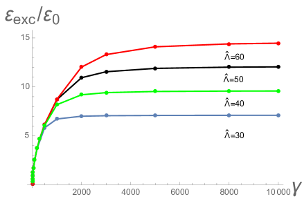
Figure 22: (Color online) Excitation energy (scaled by LHY correction to the ground state energy) following a scattering length ramp $0.5a_{f}\to a_{f}$ as a function of ramp rate $\gamma$ for different scaled momentum cutoff $\hat{\Lambda}=\Lambda\xi$ (here $\xi\equiv 1/\sqrt{2mng_{f}}$ is the coherence length). For large ramp rate $\gamma$ (fast ramp), the excitation energy ${\cal E}_{exc}$ (defined in the text) grows linearly with the UV cutoff $\Lambda$, while for small rate (slow ramp) the cutoff dependence drops out and is replaced by a square-root of the ramp rate $\gamma$.

We also verify the square-root prediction of the scaling theory for slow ramp rate, Eq.(142b), in Fig. 4, by “zooming-in” Fig. 22. The $\sigma$ (quench depth) dependence in Eq. (142b) is also confirmed by inspecting Fig. 23.

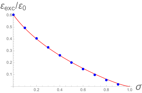
Figure 23: (Color online) Excitation energy (scaled by LHY correction to the ground state energy) following a scattering length ramp from $a_{i}\to a_{f}$ as a function of quench depth $\sigma={a_{i}}/{a_{f}}$. The blue data points are obtained for each chosen $\sigma$ at dimensionless ramp $\hat{\gamma}\equiv(1-\sigma)/(\tau ng_{f})=10$ and scaled momentum cutoff $\hat{\Lambda}=\Lambda\xi=60$; the red curve represents fitting function $y=0.58(1-x)^{3/2}$.

With this we conclude our analysis of the excitation energy and turn to the study of the dynamic analog of Tan’s contact Tan .

VIII Contact

VIII.1 Ground state contact

Contact, $C$ is a remarkable physical parameter introduced by Tan Tan , that enters in a large variety of physical observables. Most notably, it appears as a coefficient of the universal large momentum tail of the ground-state momentum distribution function

$$C = \lim_{k\to\infty}k^{4}n_{k}$$ (146)

and as a response of the ground-state energy density ${\cal E}_{gs}\equiv E_{gs}/V$ to the tuning of the scattering length, the so-called adiabatic theorem,

$$C = -{8\pi m}{}\frac{d{\cal E}_{gs}}{da^{-1}_{s}},$$ (147a)

$$= \left({mg}{}\right)^{2}\langle\hat{\psi}^{\dagger}\hat{\psi}^{\dagger}\hat{\psi}\hat{\psi}\rangle,$$ (147b)

with the second relation to the interaction energy (already noted in the previous section) obtained via the Hellmann-Feynman theorem Shankar . As we show in Appendix D.1, above can be straightforwardly evaluated in the ground state within the dilute Bogoluibov approximation refsBogoluibovContact . Though contact is quite different for fermions and bosons, in equilibrium, these relations are expected to hold independent of statistics.

The contact was first successfully measured in the ground state of stable fermionic gases, with relations experimentally verified JinRF . More recently, the contact was studied in a resonant bosonic gas via Bragg spectroscopy, utilizing the adiabatic theorem, (147a)) Wild and more directly from the large frequency $1/\omega^{3/2}$ tail (frequency analog of $1/k^{4}$ momentum tail, (146); see (69)) of the RF spectroscopy signal Wild . However, because a resonant Bose gas is fundamentally unstable and evaporates through the three-body decay, these measurements are intrinsically nonequilibrium, requiring a dynamical analysis of the contact.

VIII.2 Dynamical contact

We thus examine the contact and its associated relations for a resonant Bose gas dynamics following a quench. Immediately after the quench the states remain unchanged $|0^{-}\rangle=|0^{+}\rangle$ and only the coupling changes, $g_{i}\rightarrow g_{f}$. Thus, the relation between two forms of $C$ defined in (147a) and (147b) remains valid,

$$C_{dE}(0^{+}) = -{8\pi m}{}\frac{d{\cal E}_{f}}{da_{f}^{-1}}$$ (148)

$$= \left({mg_{f}}{}\right)^{2}\langle 0^{+}|\hat{\psi}^{\dagger}\hat{\psi}^{\dagger}\hat{\psi}\hat{\psi}|0^{+}\rangle$$

$$= \left(\frac{g_{f}}{g_{i}}\right)^{2}C_{E}(0^{-}),$$

despite the fact that $|0^{+}\rangle$ is not an eigenstate of $\hat{H}(0^{+})\equiv\hat{H}_{f}$ and thus Hellmann-Feynman theorem no longer applies.

However, the contact $C_{dE}$ is then clearly not continuous across the quench, and using (128),(134) acquires a UV cutoff dependence $\Lambda=1/r_{0}$, that drops out only in the $a_{i,f}\gg r_{0}$ limit

$$C_{dE}(0^{+}) = \left(\frac{g_{f}}{g_{i}}\right)^{2}C_{E}(0^{-}),$$ (149a)

$$= C_{E}(0^{-}),\;\;\;\mbox{$a_{i,f}\gg r_{0}$},$$

$$= \left(\frac{a_{f}}{a_{i}}\right)^{2}\left(1+\frac{4}{\pi r_{0}}(a_{f}-a_{i})\right)C_{E}(0^{-}),\;\;\;\mbox{$a_{i,f}\ll r_{0}$}$$

. (149c)

This is consistent with cutoff dependence found in the excitation energy, (137). On the other hand the momentum distribution function only depends on the state and is thus continuous across the quench. Thus, the contact $C_{n}$, defined by the large momentum tail of the distribution function, (146) is continuous across the quench and is therefore distinct from $C_{E}$.

Utilizing the analysis of Sec. IV, we next compute these contact quantities at time $t$ after the quench. We first study the contact $C_{E}(t)$ defined by the quartic interaction, (147b). Relegating the calculation details to Appendix D.2, within the Bogoluibov approximation we find

$$C_{E}(t)=(4\pi na_{f})^{2}+F_{C}(\sigma,t)C^{f}_{LHY},$$ (150)

where the $C^{f}_{LHY}$ is the LHY correction to the ground state contact for quenched Hamiltonian with $a_{f}$

$$C^{f}_{LHY}=(4\pi na_{f})^{2}\frac{64}{3\sqrt{\pi}}(na^{3}_{f})^{1/2}$$ (151)

and the time-dependent enhancement factor due to the quench is given by

$$\begin{split}F_{C}(\sigma,t)&=\frac{\sigma^{3/2}+3\sqrt{\sigma}+3\sqrt{1-\sigma}\mathrm{arccos}{\sqrt{\sigma}}}{4}\\ &\quad+\frac{3\sqrt{2}}{8}\int dyy^{2}\frac{y(1-\sigma)}{(y^{2}+2)\sqrt{y^{2}+2\sigma}}\\ &\qquad\times\cos[2\hat{t}\sqrt{y^{2}(y^{2}+2)}]\\ \end{split}$$ (152)

and illustrated in Fig. 24.

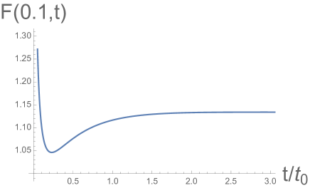
Figure 24: (Color online) Contact enhancement factor $F_{C}(\sigma,t)$ above the corresponding ground state value as a function of time following a scattering length quench $0.1a_{f}\to a_{f}$, in units of pre-thermalization time scale $t_{0}=\hbar/ng_{f}=m/(4\pi a_{f}n\hbar)$. For a typical ⁸⁵Rb experiment with $n=5\times 10^{12}cm^{-3}$, $a_{s}=1100a_{0}$, $t_{0}\approx 360\mu s$.

Immediately after the quench, at $t=0^{+}$, the quantity $F_{C}(\sigma,t)$ can be evaluated analytically, giving the contact

$$\begin{split}C_{E}(0^{+})&=(4\pi na_{f})^{2}\left[1+\frac{64}{3\sqrt{\pi}}({na_{i}^{3}})^{1/2}\right]\\ &\quad+64\pi a^{2}_{f}n^{2}\Lambda(a_{f}-a_{i}),\end{split}$$ (153)

which is the Bogoluibov limit of the general result in Eq. (149c). This UV cutoff-dependence is reflected in the large value of the numerically evaluated contact near $t=0^{+}$, in Fig. 24. As time evolves after a quench, the contact decreases dramatically within a short window of time, with the cutoff-dependence quickly vanishing. After reaching a minimum it then slowly grows to a finite steady-state value, $C_{ss}$.

At long times, the sinusoid in (152) averages out and contact reaches a steady-state value

$$\begin{split}h(\sigma)\equiv F_{C}(\sigma,t\to\infty)=\frac{\sigma^{3/2}+3\sqrt{\sigma}+3\sqrt{1-\sigma}\mathrm{arccos}{\sqrt{\sigma}}}{4}\\ \end{split}$$ (154)

plotted in Fig. 25. This steady-state contact is greater than the contact in the ground state for the same scattering length $a_{f}$.

Figure 25: (Color online) Asymptotic Contact enhancement factor $h(\sigma)\equiv F_{C}(\sigma,t\to\infty)$ following a scattering length quench $a_{i}\to a_{f}$ as a function of quench depth $\sigma={a_{i}}/{a_{f}}$. Two dots correspond to maximum enhancement $h(0)=3\pi/8$ (non-interacting initial state or unitarity final state) and minimum enhancement $h(1)=1$ (no quench), respectively.

Finally, we examine the contact associated with the tail of the momentum distribution function after the quench, which is given by Eq. (94) following a deep quench and Eq. (48) for a shallow quench, respectively. From these we straightforwardly obtain

$$\begin{split}C_{n}=\lim_{k\to\infty}k^{4}n_{k}=(4\pi a_{f}n)^{2}\left[\frac{n^{ss}_{c}}{n}+(1-\sigma)^{2}\right]\end{split}$$ (155)

and the shallow quench result is obtained by setting $n^{ss}=n$ using Bogoluibov approximation. Clearly, this is also independent of time. Thus, out of equilibrium, the three forms of the contact, $C_{n}$, $C_{E}$, $C_{dE}$ no longer coincide, like they do in the ground state.

Above analysis of various forms of contact in the nonequilibrium state thus shows that no direct relation of the coefficient of the $1/\omega^{3/2}$ tail in RF spectroscopy Wild to the equilibrium contact and its other ground state relations can be made.

IX Summary and open directions

In this manuscript we studied the dynamics of a resonant Bose gas following shallow and deep scattering length quenches and ramps, confining to a metastable regime of a positive scattering length. Utilizing a dynamic field theory extension of the Bogoluibov theory, which self-consistently accounts for a large depletion and a time-dependent condensate density, we approximately solved for the full post-quench evolution of the system. From this we then computed a variety of physical observables, such as the evolution of the momentum distribution function, the associated condensate depletion, the time-dependent structure function, the RF spectroscopy signal, the excitation energy and various forms of a “nonequilibrium contact”. We found, that following initial transient dynamics, the Bose gas exhibits a pre-thermalization to a stationary state (characterized e.g., by a stationary momentum distribution function) that differs qualitatively from the corresponding ground state. Because of integrability of the approximate model, that does not include quasi-particles scattering, the system never exhibits full thermalization to a ground state. Despite the simplicity of our model and approximate analysis, our results are in reasonable qualitative agreement with recent JILA experiments Makotyn .

Although we made significant progress in understanding the post-quench dynamics of a resonant Bose system, our work leaves a number questions for a future investigation. Our present study utilized a single-channel model and focussed on the upper-branch physics with a tunable positive scattering length, thereby neglecting the closed molecular channel. The latter may in fact be quite significant, enriching the dynamics by allowing coherent condensate oscillations not only into pairs of atomic quasi-particles in the upper branch, but also into molecular condensate and molecular quasi-particles. This extension can be quite naturally treated within a two-channel model, where the closed molecular channel is explicitly included. It would allow one to address the dynamics not only within the superfluid phase but across quantum and classical phase transitions, most notably across the quantum Ising transition between atomic and molecular superfluids and throughout the atomic-molecular phase diagram RPWmolecularBECprl04 ; StoofMolecularBEC04 ; RPWmolecularBECpra08 .

Another crucial ingredient missing in our model is the quasi-particle scattering. This is responsible for a time-independent quasi-particle momentum distribution function, that is completely fixed by the initial state, characterized by $a_{i}$ and the final scattering length $a_{f}$. This feature is responsible for the absence of thermalization of the system. It is thus desirable to extend the present model to include quasi-particle scattering, that can be handled through the Boltzmann equation for the quasi-particle distribution function. In such a generalized model, the dynamics of the atomic observables (e.g., atomic momentum distribution and structure functions) will consist of two contributions, Heisenberg evolution of atoms due to quasi-particle unitary dynamics, coupled to the evolution of the quasi-particle momentum distribution function governed by the Boltzmann equation with collision integrals. We expect that such dynamics will exhibit a second, longer time scale, set by the quasi-particle scattering that will lead to true long-time thermalization.

Finally, to treat the effects of interactions more systematically, it is desirable to have a full nonequilibrium Schwinger-Keldysh field theoretic formulation. We leave these and a number of other open question for future research LRunpublished .

Appendix A Energy conservation

In this appendix we study the time evolution of the total energy following a deep quench. Although energy is conserved under exact unitary evolution of a closed system, it is less clear whether it remains so for the time-dependent self-consistent Bogoluibov approximation employed in deep quenches. We demonstrate below that within this approximation, that neglects anomalous averages of finite momentum excitations, the total energy is indeed conserved.

To this end we study the time derivative of the full time-dependent Hamiltonian, including the constant mean-field parts derived in Sec. II, (32). It is given by

$$\begin{split}\hat{H}_{total}&=\sum_{{\bf k}\neq 0}\bigg{[}(\epsilon_{k}+gn_{c}(t))\hat{a}^{\dagger}_{\bf k}\hat{a}_{\bf k}+\frac{g}{2}n_{c}(t)(\hat{a}_{\bf k}\hat{a}_{-{\bf k}}+\hat{a}^{\dagger}_{\bf k}\hat{a}^{\dagger}_{-{\bf k}})\bigg{]}\\ &\quad+g[n_{c}(t){n}_{d}(t)+\frac{1}{2}n^{2}_{c}(t)+{n}^{2}_{d}(t)],\end{split}$$ (156)

where $g$ is the final interaction $g_{f}$ to which the system is quenched, and the energy is evaluated as

$$E_{total}(t)=\langle 0^{-}|\hat{H}_{total}(t)|0^{-}\rangle=E_{1}(t)+E_{2}(t)+E_{3}(t).$$ (157)

The time derivative of last mean-field term, $E_{3}$ is given by

$$\begin{split}\frac{dE_{3}}{dt}&=g[\dot{n}_{c}{n}_{d}+n_{c}\dot{{n}}_{d}+n_{c}\dot{n}_{c}+2{n}_{d}\dot{{n}}_{d}],\\ &=g{n}_{d}\dot{{n}}_{d},\end{split}$$ (158)

where we used the atom conservation constraint $n=n_{c}(t)+n_{d}(t)$, giving $\dot{n}_{c}(t)+\dot{n}_{d}(t)=0$.

A time derivative of the first term $E_{1}(t)$ is

$$\begin{split}\frac{dE_{1}}{dt}&\equiv\frac{d}{dt}\sum_{{\bf k}\neq 0}\left(\epsilon_{k}+gn_{c}(t)\right)\langle 0^{-}|\hat{a}^{\dagger}_{\bf k}(t)\hat{a}_{\bf k}(t)|0^{-}\rangle,\\ &=\sum_{{\bf k}\neq 0}g\dot{n}_{c}\langle\hat{a}^{\dagger}_{\bf k}\hat{a}_{\bf k}\rangle+(\epsilon_{k}+gn_{c}(t))\langle\dot{\hat{a}}^{\dagger}_{\bf k}\hat{a}_{\bf k}+\hat{a}^{\dagger}_{\bf k}\dot{\hat{a}}_{\bf k}\rangle,\end{split}$$ (159)

and of the second term $E_{2}(t)$

$$\begin{split}\frac{dE_{2}}{dt}&\equiv\frac{g}{2}\frac{d}{dt}\sum_{{\bf k}\neq 0}n_{c}(t)\langle 0^{-}|\hat{a}_{\bf k}(t)\hat{a}_{-{\bf k}}(t)+\hat{a}^{\dagger}_{\bf k}(t)\hat{a}^{\dagger}_{-{\bf k}}(t)|0^{-}\rangle,\\ &=\sum_{{\bf k}\neq 0}\frac{g}{2}\dot{n}_{c}\langle\hat{a}_{\bf k}\hat{a}_{-{\bf k}}+\hat{a}^{\dagger}_{\bf k}\hat{a}^{\dagger}_{-{\bf k}}\rangle+\frac{g}{2}n_{c}\langle\dot{\hat{a}}_{\bf k}\hat{a}_{-{\bf k}}+\hat{a}_{\bf k}\dot{\hat{a}}_{-{\bf k}}\\ &\quad+\dot{\hat{a}}^{\dagger}_{\bf k}\hat{a}^{\dagger}_{-{\bf k}}+\hat{a}^{\dagger}_{\bf k}\dot{\hat{a}}^{\dagger}_{-{\bf k}}\rangle.\end{split}$$ (160)

Using the Heisenberg equation of motion to eliminate time derivatives of atom operators we find

$$\begin{split}\dot{\hat{a}}_{\bf k}&=\frac{1}{i}[(\epsilon_{k}+gn_{c})\hat{a}_{\bf k}+gn_{c}\hat{a}^{\dagger}_{-{\bf k}}],\\ \dot{\hat{a}}_{-{\bf k}}&=\frac{1}{i}[(\epsilon_{k}+gn_{c})\hat{a}_{-{\bf k}}+gn_{c}\hat{a}^{\dagger}_{{\bf k}}].\\ \end{split}$$ (161)

With this (159) and (160) reduce to

$$\begin{split}\frac{dE_{1}}{dt}=g\dot{n}_{c}n_{d}+\frac{1}{i}\sum_{{\bf k}\neq 0}gn_{c}(\epsilon_{k}+gn_{c})\langle\hat{a}^{\dagger}_{{\bf k}}\hat{a}^{\dagger}_{-{\bf k}}-\hat{a}_{{\bf k}}\hat{a}_{-{\bf k}}\rangle\end{split}$$ (162)

and

$$\begin{split}\frac{dE_{2}}{dt}&=\sum_{{\bf k}\neq 0}\frac{g}{2}\dot{n}_{c}\langle\hat{a}_{\bf k}\hat{a}_{-{\bf k}}+\hat{a}^{\dagger}_{\bf k}\hat{a}^{\dagger}_{-{\bf k}}\rangle\\ &\quad+\frac{gn_{c}}{i}((\epsilon_{k}+gn_{c})\langle\hat{a}_{\bf k}\hat{a}_{-{\bf k}}-\hat{a}^{\dagger}_{\bf k}\hat{a}^{\dagger}_{-{\bf k}}\rangle.\end{split}$$ (163)

For the total energy we then obtain,

$$\begin{split}\frac{dE_{total}}{dt}&=\sum_{{\bf k}\neq 0}\frac{g}{2}\dot{n}_{c}[\langle\hat{a}_{\bf k}\hat{a}_{-{\bf k}}\rangle+\langle\hat{a}^{\dagger}_{\bf k}\hat{a}^{\dagger}_{-{\bf k}}\rangle]\approx 0,\\ \end{split}$$ (164)

where in the last approximation we neglected anomalous correlator of excited atoms. More precisely, following Sotiriadis and Cardy SotiriadisCardy10 , we observe that while the conventional definition of the energy is not conserved, the shifted one $E_{shifted}\equiv E_{total}-\frac{g}{2}\int dt\dot{n}_{c}[\langle\hat{a}_{\bf k}\hat{a}_{-{\bf k}}\rangle+\langle\hat{a}^{\dagger}_{\bf k}\hat{a}^{\dagger}_{-{\bf k}}\rangle]$ approximately is.

Appendix B $U(t)$ for quasi-adiabatic approximation

In this seciton, we fill in the technical details leading to $U(t)$ for quasi-adiabatic approximation in Eq. (92). The operator part of time-dependent Hamiltonian is

$$\begin{split}\hat{H}(t)&=\frac{1}{2}\sum_{{\bf k}\neq 0}((\epsilon_{k}+n_{c}(t)g_{f})(\hat{a}^{\dagger}_{k}\hat{a}_{\bf k}+\hat{a}^{\dagger}_{-{\bf k}}\hat{a}_{-{\bf k}})\\ &\quad+n_{c}(t)g_{f}(\hat{a}^{\dagger}_{\bf k}\hat{a}^{\dagger}_{-{\bf k}}+\hat{a}_{\bf k}\hat{a}_{-{\bf k}})).\end{split}$$ (165)

It can be instantaneously diagonalized by

$$\begin{pmatrix}\hat{a}_{\bf k}(t)\\ \hat{a}^{\dagger}_{-{\bf k}}(t)\end{pmatrix}=\begin{pmatrix}u_{k}(t)&v_{k}(t)\\ v_{k}(t)&u_{k}(t)\end{pmatrix}\begin{pmatrix}\hat{\gamma}_{\bf k}(t)\\ \hat{\gamma}^{\dagger}_{-{\bf k}}(t)\end{pmatrix},$$ (166)

and rewritten as

$$\begin{split}\hat{H}(t)=-\frac{1}{2}\sum_{{\bf k}\neq 0}(\epsilon_{k}+n_{c}(t)g-E_{kf}(t))\\ +\frac{1}{2}\sum_{{\bf k}\neq 0}E_{kf}(t)(\hat{\gamma}^{\dagger}_{\bf k}\hat{\gamma}_{\bf k}+\hat{\gamma}^{\dagger}_{-{\bf k}}\hat{\gamma}_{-{\bf k}}),\end{split}$$ (167)

where

$$\begin{split}u_{k}(t)&=\sqrt{\frac{1}{2}(\frac{\epsilon_{k}+g_{f}n_{c}(t)}{E_{k}(t)}+1)},\\ v_{k}(t)&=-\sqrt{\frac{1}{2}(\frac{\epsilon_{k}+g_{f}n_{c}(t)}{E_{k}(t)}-1)},\\ E_{kf}(t)&=\sqrt{\epsilon_{k}(\epsilon_{k}+2g_{f}n_{c}(t))}.\end{split}$$ (168)

The time-dependence of $\hat{\gamma}^{\dagger}_{\bf k}(t)$ and $\hat{\gamma}_{\bf k}(t)$ is obtained from the Heisenberg equation of motion,

$$\frac{d\hat{\gamma}_{\bf k}}{dt}=i[\hat{\gamma}_{\bf k},\hat{H}]+\frac{\partial\hat{\gamma}_{\bf k}}{\partial t},$$ (169)

where the last term accounts for the explicit time-dependence in Hamiltonian. To compute it we first express $\hat{\gamma}^{\dagger}_{\bf k}(t)$ and $\hat{\gamma}_{\bf k}(t)$ in terms of $\hat{a}^{\dagger}_{\bf k}(t)$ and $\hat{a}_{\bf k}(t)$.

$$\begin{pmatrix}\hat{\gamma}_{\bf k}(t)\\ \hat{\gamma}^{\dagger}_{-{\bf k}}(t)\end{pmatrix}=\begin{pmatrix}u_{k}(t)&-v_{k}(t)\\ -v_{k}(t)&u_{k}(t)\end{pmatrix}\begin{pmatrix}\hat{a}_{\bf k}(t)\\ \hat{a}^{\dagger}_{-{\bf k}}(t)\end{pmatrix},$$ (170)

Then

$$\begin{split}\frac{\partial}{\partial t}\begin{pmatrix}\hat{\gamma}_{\bf k}(t)\\ \hat{\gamma}^{\dagger}_{-{\bf k}}(t)\end{pmatrix}&=\begin{pmatrix}\dot{u}_{k}(t)&-\dot{v}_{k}(t)\\ -\dot{v}_{k}(t)&\dot{u}_{k}(t)\end{pmatrix}\begin{pmatrix}\hat{a}_{\bf k}(t)\\ \hat{a}^{\dagger}_{-{\bf k}}(t)\end{pmatrix},\\ &=\begin{pmatrix}\dot{u}_{k}(t)&-\dot{v}_{k}(t)\\ -\dot{v}_{k}(t)&\dot{u}_{k}(t)\end{pmatrix}\begin{pmatrix}u_{k}(t)&v_{k}(t)\\ v_{k}(t)&u_{k}(t)\end{pmatrix}\begin{pmatrix}\hat{\gamma}_{\bf k}(t)\\ \hat{\gamma}^{\dagger}_{-{\bf k}}(t)\end{pmatrix},\\ &=\begin{pmatrix}0&\frac{g\dot{n}_{c}(t)\epsilon_{k}}{2E^{2}_{kf}}\\ \frac{g\dot{n}_{c}(t)\epsilon_{k}}{2E^{2}_{kf}}&0\end{pmatrix}\begin{pmatrix}\hat{\gamma}_{\bf k}(t)\\ \hat{\gamma}^{\dagger}_{-{\bf k}}(t)\end{pmatrix}.\end{split}$$ (171)

Now the equation of motions become

$$\frac{d}{dt}\begin{pmatrix}\hat{\gamma}_{\bf k}(t)\\ \hat{\gamma}^{\dagger}_{-{\bf k}}(t)\end{pmatrix}=\begin{pmatrix}-iE_{kf}(t)&\frac{g\dot{n}_{c}(t)\epsilon_{k}}{2E^{2}_{kf}}\\ \frac{g\dot{n}_{c}(t)\epsilon_{k}}{2E^{2}_{kf}}&iE_{kf}(t)\end{pmatrix}\begin{pmatrix}\hat{\gamma}_{\bf k}(t)\\ \hat{\gamma}^{\dagger}_{-{\bf k}}(t)\end{pmatrix}.$$ (172)

Assuming $\dot{n}_{c}(t)$ changes slowly compared to other timescales (or more explicitly ${\dot{n}_{c}(t)}/{n}\ll{E^{3}_{kf}}/(\hbar ng\epsilon_{k})$), we can ignore the off-diagonal terms in (172) and have

$$\frac{d}{dt}\begin{pmatrix}\hat{\gamma}_{\bf k}(t)\\ \hat{\gamma}^{\dagger}_{-{\bf k}}(t)\end{pmatrix}\approx\begin{pmatrix}-iE_{kf}(t)&0\\ 0&iE_{kf}(t)\end{pmatrix}\begin{pmatrix}\hat{\gamma}_{\bf k}(t)\\ \hat{\gamma}^{\dagger}_{-{\bf k}}(t)\end{pmatrix},$$ (173)

from which we can solve $\hat{\gamma}^{\dagger}_{\bf k}(t)$ and $\hat{\gamma}_{\bf k}(t)$ as

$$\hat{\gamma}_{\bf k}(t)=\hat{\gamma}_{\bf k}e^{-i\int_{0}^{t}dt^{\prime}E_{kf}(t^{\prime})},\;\;\;\;\;\;\;\hat{\gamma}^{\dagger}_{-{\bf k}}(t)=\hat{\gamma}^{\dagger}_{-{\bf k}}e^{i\int_{0}^{t}dt^{\prime}E_{kf}(t^{\prime})},$$ (174)

thus

$$\begin{split}\begin{pmatrix}\hat{a}_{\bf k}(t)\\ \hat{a}^{\dagger}_{-{\bf k}}(t)\end{pmatrix}&=\begin{pmatrix}u_{k}(t)&v_{k}(t)\\ v_{k}(t)&u_{k}(t)\end{pmatrix}\begin{pmatrix}e^{-i\int_{0}^{t}dtE_{kf}(t^{\prime})}&0\\ 0&e^{i\int_{0}^{t}dtE_{kf}(t^{\prime})}\end{pmatrix}\begin{pmatrix}\hat{\gamma}_{\bf k}\\ \hat{\gamma}^{\dagger}_{-{\bf k}}\end{pmatrix},\\ &=\begin{pmatrix}u_{k}(t)e^{-i\int_{0}^{t}dtE_{kf}(t^{\prime})}&v_{k}(t)e^{i\int_{0}^{t}dtE_{kf}(t^{\prime})}\\ v_{k}(t)e^{-i\int_{0}^{t}dtE_{kf}(t^{\prime})}&u_{k}(t)e^{i\int_{0}^{t}dtE_{kf}(t^{\prime})}\end{pmatrix}\begin{pmatrix}\hat{\gamma}_{\bf k}\\ \hat{\gamma}^{\dagger}_{-{\bf k}}\end{pmatrix}.\end{split}$$ (175)

Comparing this with Eq. (87) , we find

$$\begin{split}U(t)=\begin{pmatrix}u_{k}(t)e^{-i\int_{0}^{t}dtE_{kf}(t^{\prime})}&v_{k}(t)e^{i\int_{0}^{t}dtE_{kf}(t^{\prime})}\\ v_{k}(t)e^{-i\int_{0}^{t}dtE_{kf}(t^{\prime})}&u_{k}(t)e^{i\int_{0}^{t}dtE_{kf}(t^{\prime})}\end{pmatrix}.\end{split}$$ (176)

Appendix C Energy after quench

In this section we evaluate the total energy of the system after the sudden quench. Separating the energy into kinectic part and interaciton part

$$\begin{split}\langle 0^{-}|\hat{H}^{f}|0^{-}\rangle=\langle 0^{-}|\hat{H}^{f}_{KE}|0^{-}\rangle+\langle 0^{-}|\hat{H}^{f}_{int}|0^{-}\rangle,\end{split}$$ (177)

with

$$\begin{split}\hat{H}^{f}_{KE}=\frac{1}{2}\sum_{{\bf k}\neq 0}\epsilon^{0}_{k}(\hat{a}^{\dagger}_{\bf k}\hat{a}_{\bf k}+\hat{a}^{\dagger}_{-{\bf k}}\hat{a}_{-{\bf k}}),\\ \end{split}$$ (178)

$$\begin{split}\hat{H}^{f}_{int}=\frac{1}{2}Vg_{f}n^{2}+\frac{1}{2}\sum_{{\bf k}\neq 0}[ng_{f}(\hat{a}^{\dagger}_{\bf k}\hat{a}_{\bf k}+\hat{a}^{\dagger}_{-{\bf k}}\hat{a}_{-{\bf k}})+ng_{f}(\hat{a}^{\dagger}_{\bf k}\hat{a}^{\dagger}_{-{\bf k}}+\hat{a}_{\bf k}\hat{a}_{-{\bf k}})],\end{split}$$ (179)

we then use Bogoluibov transformation to evaluate them respectively by expressing $\hat{a}_{\bf k}$ in terms of pre-quench basis $\hat{\alpha}_{\bf k}$, obtaining

$$\begin{split}\hat{H}_{KE}=\sum_{{\bf k}\neq 0}\epsilon_{k}\hat{a}^{\dagger}_{\bf k}\hat{a}_{\bf k}=\sum_{{\bf k}\neq 0}\epsilon_{k}\left(|u_{k}|^{2}\hat{\alpha}^{\dagger}_{\bf k}\hat{\alpha}_{\bf k}-u^{*}_{k}v_{k}\hat{\alpha}^{\dagger}_{\bf k}\hat{\alpha}^{\dagger}_{-{\bf k}}-u_{k}v^{*}_{k}\hat{\alpha}_{-{\bf k}}\hat{\alpha}_{\bf k}+|v_{k}|^{2}\hat{\alpha}_{-{\bf k}}\hat{\alpha}^{\dagger}_{-{\bf k}}\right),\end{split}$$ (180)

and

$$\begin{split}\hat{H}_{int}&=\frac{1}{2}Vg_{f}n^{2}+ng_{f}\sum_{{\bf k}\neq 0}[|v_{k}|^{2}-\frac{1}{2}(u^{*}_{k}v_{k}+u_{k}v_{k}^{*})]\\ &\quad+\frac{1}{2}ng_{f}\sum_{{\bf k}\neq 0}\left[\left(|u^{2}_{k}|+|v^{2}_{k}|-(u^{*}_{k}v_{k}+u_{k}v^{*}_{k})\right)(\hat{\alpha}^{\dagger}_{\bf k}\hat{\alpha}_{{\bf k}}+\hat{\alpha}^{\dagger}_{-{\bf k}}\hat{\alpha}_{-{\bf k}})+(u^{2}_{k}+v^{2}_{k}-2u_{k}v_{k})(\hat{\alpha}^{\dagger}_{\bf k}\hat{\alpha}^{\dagger}_{-{\bf k}}+\hat{\alpha}_{{\bf k}}\hat{\alpha}_{-{\bf k}})\right].\end{split}$$ (181)

Since $\hat{\alpha}_{\bf k}|0^{-}\rangle=0$, we have

$$\langle 0^{-}|\hat{H}_{KE}|0^{-}\rangle=\sum_{{\bf k}\neq 0}\epsilon_{k}|v_{k}|^{2},$$ (182)

and

$$\begin{split}&\langle 0^{-}|\hat{H}^{f}_{int}|0^{-}\rangle=\frac{1}{2}V\tilde{g}_{f}n^{2}+n\tilde{g}_{f}\sum_{{\bf k}\neq 0}\left[|v_{k}|^{2}-\frac{1}{2}(u^{*}_{k}v_{k}+u_{k}v_{k}^{*})+\frac{n\tilde{g}_{f}}{4\epsilon_{k}}\right],\end{split}$$ (183)

during which coupling $g$ has been expanded to second order

$$\begin{split}g=\frac{4\pi a}{m}+\frac{(4\pi a)^{2}}{m^{2}V}\sum_{{\bf k}\neq 0}\frac{1}{2\epsilon_{k}}\equiv\tilde{g}+\frac{\tilde{g}^{2}}{V}\sum_{{\bf k}\neq 0}\frac{1}{2\epsilon_{k}}.\end{split}$$ (184)

Therefore, the total energy is

$$\begin{split}E_{tot}(t=0^{+})&=\langle 0^{-}|\hat{H}_{KE}+\hat{H}_{int}|0^{-}\rangle,\\ &=\frac{1}{2}V\tilde{g}_{f}n^{2}+n\tilde{g}_{f}\sum_{{\bf k}\neq 0}\left[\left(\frac{\epsilon_{k}}{n\tilde{g}}+1\right)|v_{k}|^{2}-\frac{1}{2}(u^{*}_{k}v_{k}+u_{k}v_{k}^{*})+\frac{n\tilde{g}_{f}}{4\epsilon_{k}}\right],\\ &=\frac{2\pi na_{f}}{m}+\frac{32\sqrt{2\pi}na_{f}}{m}({na^{3}_{f}})^{1/2}\int dkk^{2}\left[(k^{2}+1)|v_{k}|^{2}-\frac{1}{2}(u_{k}v^{*}_{k}+v_{k}u^{*}_{k})+\frac{1}{4k^{2}}\right].\end{split}$$ (185)

For a sudden quench, the expressions for $u_{k}$ and $v_{k}$ are simple

$$\begin{split}u_{k}&=\sqrt{\frac{1}{2}(\frac{\epsilon_{k}+n\tilde{g}_{i}}{\sqrt{\epsilon_{k}(\epsilon_{k}+2n\tilde{g}_{i})}}+1)},\\ v_{k}&=-\sqrt{\frac{1}{2}(\frac{\epsilon_{k}+n\tilde{g}_{i}}{\sqrt{\epsilon_{k}(\epsilon_{k}+2n\tilde{g}_{i})}}-1)}.\\ \end{split}$$ (186)

Plugging Eq. (186) into (182) and (183), we obtain the kinetic energy as

$$\begin{split}\langle 0^{-}|\hat{H}_{KE}|0^{-}\rangle&=\sum_{{\bf k}\neq 0}\frac{1}{2}\epsilon_{k}(\frac{\epsilon_{k}+n\tilde{g}_{i}}{\sqrt{\epsilon_{k}(\epsilon_{k}+2n\tilde{g}_{i})}}-1),\\ &=\frac{1}{2}n\tilde{g}_{i}(2m\tilde{g}_{i}n)^{3/2}\frac{4\pi V}{(2\pi)^{3}}\int dyy^{2}\left[\frac{y^{2}+1}{\sqrt{y^{2}(y^{2}+2)}}-1\right],\\ &=N\frac{4a_{i}n}{m}\Lambda a_{i}-\frac{128\sqrt{\pi}a_{i}n}{5m}N({na^{3}_{i}})^{1/2},\end{split}$$ (187)

the interaction energy as

$$\begin{split}\langle 0^{-}|\hat{H}^{f}_{int}|0^{-}\rangle&=\frac{1}{2}V\tilde{g}_{f}n^{2}+\frac{1}{2}n\tilde{g}_{f}\sum_{{\bf k}\neq 0}(\epsilon_{k}/\sqrt{\epsilon_{k}(\epsilon_{k}+n\tilde{g}_{f})}-1+n\tilde{g}_{f}/2\epsilon_{k}),\\ &=\frac{1}{2}Vn^{2}\tilde{g}_{f}+\frac{1}{2}n\tilde{g}_{f}(2m\tilde{g}_{f}n)^{\frac{3}{2}}\frac{4\pi V}{(2\pi)^{3}}\int dyy^{2}\left(\frac{y}{\sqrt{y^{2}+2\sigma}}-1+\frac{1}{2y^{2}}\right),\\ &=\frac{2\pi a_{f}n}{m}N\left[1+\frac{64}{3}(\frac{na^{3}_{i}}{\pi})^{\frac{1}{2}}\right]+(1-2\sigma)N\frac{4a_{f}n}{m}\Lambda a_{f},\end{split}$$ (188)

and the total energy as

$$\begin{split}E_{tot}&=\langle 0^{-}|\hat{H}_{KE}+\hat{H}_{int}|0^{-}\rangle=\frac{4(1-\sigma)^{2}na_{f}}{m}Na_{f}\Lambda-\frac{128\sqrt{\pi}na_{i}}{5m}N({na^{3}_{i}})^{1/2}+\frac{2\pi na_{f}}{m}N\left[1+\frac{64}{3\sqrt{\pi}}({na^{3}_{i}})^{1/2}\right],\end{split}$$ (189)

which is Eq. (126) in the text. The ground state energy can be easily obtained by setting $\sigma=1$, and one obtains

$$\begin{split}E_{tot}=\frac{2\pi a_{s}n}{m}N[1+\frac{128}{15}(\frac{na^{3}_{s}}{\pi})^{\frac{1}{2}}].\\ \end{split}$$ (190)

as the cutoff dependences of kinetic energy and interaction energy cancel each other, recovering the LHY result as expected.

Appendix D Contact

D.1 Ground state contact

In this paper, we follow E. Braaten et.al Braaten and take the working definition of contact to be

$$\begin{split}C=(mg)^{2}\langle\int dr\hat{\psi}^{\dagger}(r,t)\hat{\psi}^{\dagger}(r,t)\hat{\psi}(r,t)\hat{\psi}(r,t))\rangle=2m^{2}g\langle\hat{H}_{int}\rangle/V.\end{split}$$ (191)

At $T=0$ for $na^{3}_{s}\ll 1$, the interaction energy of Bose gas is given in Appendix C. For ground state, $\langle O|\hat{H}_{int}|O\rangle$ can be evaluated by applying $\sigma=1$ to Eq. (188), which gives

$$\begin{split}\langle O|\hat{H}_{int}|O\rangle&=\frac{2\pi a_{s}Nn}{m}\left[1+\frac{64}{3\sqrt{\pi}}(na^{3}_{s})^{1/2}\right]-\frac{4\Lambda a^{2}_{s}Nn}{m},\\ &=2Nn/m\left[a_{s}\pi\left(1+\frac{64}{3\sqrt{\pi}}(na^{3}_{s})^{1/2}\right)-2a^{2}_{s}\Lambda\right].\end{split}$$ (192)

The last term contains the same divergence as the bare interaction $g$, and we show below they exactly cancel each other to give a finite contact.

$$\begin{split}C&=2m^{2}g\langle O|\hat{H}_{int}|O\rangle/V,\\ &=2m^{2}\left(\frac{4\pi a_{s}}{m}+\frac{8\Lambda a^{2}_{s}}{m}\right)\langle O|\hat{H}_{int}|O\rangle/V,\\ &=8m(\pi a_{s}+2\Lambda a^{2}_{s})\langle O|\hat{H}_{int}|O\rangle/V,\\ &=(4\pi a_{s})^{2}n^{2}\left[1+\frac{64}{3\sqrt{\pi}}({na^{3}_{s}})^{1/2}+\frac{128}{3{\pi}^{3/2}}a_{s}\Lambda({na^{3}_{s}})^{1/2}+O(\Lambda^{2}a^{2}_{s})\right].\end{split}$$ (193)

Thus to the order of $(na^{3}_{s})^{1/2}$, the contact value for ground state at $T=0$ is

$$\begin{split}C=(4\pi a_{s})^{2}nN\left[1+\frac{64}{3\sqrt{\pi}}({na^{3}_{s}})^{1/2}\right].\\ \end{split}$$ (194)

For bosons in thermal equilibrium, one central Tan’s relation is the adiabatic theorem, which relates the energy change with respect to scattering length to the contact. The theorem states the following thing

$$\begin{split}C={8\pi ma^{2}_{s}}\frac{{d\cal E}_{gs}}{da_{s}}.\\ \end{split}$$ (195)

Since the ground state energy is given by Eq. (116), it is straightforward to show that

$$\begin{split}{8\pi ma^{2}_{s}}\frac{d{\cal E}_{gs}}{da_{s}}=(4\pi a_{s}n)^{2}\left[1+\frac{64}{3\sqrt{\pi}}({na^{3}_{s}})^{\frac{1}{2}}\right].\end{split}$$ (196)

Thus we have verified the adiabatic theorem in ground state.

Another important Tan’s relation is the momentum theorem, which relates contact to the high momentum tail of the momentum distribution function

$$\begin{split}C=\lim_{k\to\infty}k^{4}n_{k}.\end{split}$$ (197)

For ground state at $T=0$, momentum distribution $n_{k}$ is given by Eq. (21), giving

$$\begin{split}\lim_{k\to\infty}k^{4}n_{k}=C_{0}+O(1/k^{2}),\end{split}$$ (198)

with $C_{0}=(4\pi a_{s}n)^{2}$. Thus we recover the lowest order of contact obtained in Eq. (194).

We can also generalize the contact to large $na_{s}^{3}$ case. From Eq. (32), the ground state energy is modified as

$$\begin{split}{\cal E}_{gs}&=\langle O|\hat{H}_{total}|O\rangle\\ &=\frac{2\pi a_{s}Vn^{2}}{m}\left[1+\left(\frac{{n}_{d}}{n}\right)^{2}+\frac{128({na^{3}_{s}})^{1/2}}{15\sqrt{\pi}}\left(\frac{{n}_{c}}{n}\right)^{5/2}\right].\end{split}$$ (199)

Then the adiabatic theorem gives

$$\begin{split}C&=8\pi ma^{2}_{s}\frac{d{\cal E}_{gs}}{da_{s}}\\ &=(4\pi a_{s}n)^{2}\left[1+\left(\frac{{n}_{d}}{n}\right)^{2}+\frac{64({na^{3}_{s}})^{1/2}}{3\sqrt{\pi}}\left(\frac{n_{c}}{n}\right)^{5/2}\right].\end{split}$$ (200)

It is straightforward to verify that this also agrees with contact obtained via Eq. (191). Here, condensate density $n_{c}$ and depletion density $n_{d}$ are determined self-consistently by Eq. (34).

D.2 Dynamical contact

An important quantity to determine dynamical contact is the interaction energy $\langle 0^{-}|\hat{H}^{f}_{int}|0^{-}\rangle$. In this section, still assuming a sudden quench, we further study the dynamics of interaction energy and focus on its asymptotic long time limit, and use it to construct the dynamical contact as in Eq. (191). Using Eq. (36a) to decompose $\hat{a}_{k}$ into post-quench basis $\hat{\beta}_{k}(t)$, as $\hat{\beta}_{k}(t)$ evolve simply according to Eq. (42), combined with Eq. (179), we obtain

$$\begin{split}&\langle 0^{-}|\hat{H}^{f}_{int}|0^{-}\rangle\\ &=\frac{1}{2}Vg_{f}n^{2}-\frac{1}{2}\sum_{{\bf k}\neq 0}ng\frac{\epsilon_{k}+2ng_{f}-\sqrt{\epsilon_{k}(\epsilon_{k}+2ng_{f})}}{\epsilon_{k}+2ng_{f}}+\frac{1}{2}\sum_{{\bf k}\neq 0}\frac{\epsilon_{k}gn}{\sqrt{\epsilon_{k}(\epsilon_{k}+2ng_{f})}}[\langle\beta^{\dagger}_{\bf k}\beta_{\bf k}\rangle+\langle\beta^{\dagger}_{-{\bf k}}\beta_{-{\bf k}}\rangle\\ &\quad+\langle\beta^{\dagger}_{{\bf k}}\beta^{\dagger}_{-{\bf k}}\rangle e^{2iE_{k}t}+\langle\beta_{{\bf k}}\beta_{-{\bf k}}\rangle e^{-2iE_{k}t},]\\ &=\frac{1}{2}Vg_{f}n^{2}+\frac{(n\tilde{g}_{f})^{2}}{4\epsilon_{k}}-\frac{1}{2}\sum_{{\bf k}\neq 0}ng_{f}\frac{\epsilon_{k}+2ng_{f}-\sqrt{\epsilon_{k}(\epsilon_{k}+2ng_{f})}}{\epsilon_{k}+2ng_{f}}+\sum_{{\bf k}\neq 0}\frac{1}{2}\epsilon_{k}ng_{f}[\frac{\epsilon_{k}+ng_{f}+ng_{i}-\sqrt{(\epsilon_{k}+2ng_{i})(\epsilon_{k}+2ng_{f})}}{(\epsilon_{k}+2ng_{f})\sqrt{\epsilon_{k}(\epsilon_{k}+2ng_{i})}},\\ &\quad+\frac{n(g_{f}-g_{i})}{(\epsilon_{k}+2ng_{f})\sqrt{\epsilon_{k}(\epsilon_{k}+2ng_{i})}}\cos[2t\sqrt{\epsilon_{k}(\epsilon_{k}+2ng_{f})}].\end{split}$$ (201)

Rescaling time and momentum and taking the integral, we obtain

$$\begin{split}\langle 0^{-}|\hat{H}^{f}_{int}|0^{-}\rangle&=\frac{1}{2}Ng_{f}n+\frac{1}{2}ng_{f}(2mg_{f}n)^{\frac{3}{2}}\frac{4\pi V}{(2\pi)^{3}}\int dyy^{2}\\ &\quad\times[y\frac{y^{2}+1+\sigma-\sqrt{(y^{2}+2\sigma)(y^{2}+2)}}{(y^{2}+2)\sqrt{y^{2}+2\sigma}}+\frac{y}{\sqrt{y^{2}+2\sigma}}-1+\frac{1}{2y^{2}}+\frac{y(1-\sigma)}{(y^{2}+2)\sqrt{y^{2}+2\sigma}}\cos(2\hat{t}\sqrt{y^{2}(y^{2}+2)}]\\ &=\frac{2Nna_{f}\pi}{m}[1+F_{C}(\sigma,t)\frac{64}{3\sqrt{\pi}}(na^{3}_{f})^{1/2})]-\frac{4Nna^{2}_{f}\Lambda}{m},\\ \end{split}$$ (202)

where $F_{C}(\sigma,t)=h(\sigma)+T(t,\sigma,\Lambda)$ and

$$\begin{split}h(\sigma)=\frac{{\sigma}^{3/2}+3\sqrt{\sigma}+3\sqrt{1-\sigma}\mathrm{arccos}{\sqrt{\sigma}}}{4},\end{split}$$ (203)

$$\begin{split}T(t,\sigma,\Lambda)=\frac{3\sqrt{2}}{8}\int dyy^{2}\frac{y(1-\sigma)}{(y^{2}+2)\sqrt{y^{2}+2\sigma}}\times\cos[2\hat{t}\sqrt{y^{2}(y^{2}+2)}].\\ \end{split}$$ (204)

Following Eq. (193), to the order of $(na^{3})^{1/2}$ we obtain the dynamical contact after a quench,

$$C_{E}(t)=(4\pi na_{f})^{2}+F_{C}(\sigma,t)C^{f}_{LHY},$$ (205)

given in Eq. (150) of the main text. In the asymptotically long time limit, $T(t\to\infty,\sigma,\Lambda)\to 0$.

D.3 RF spectroscopy

In this appendix, we dervie Eq. (68) of Sec. IV.3. With $\hat{J}_{I}(t)=e^{i\int_{0}^{t}dt^{\prime}\hat{H}_{0}}\hat{J}e^{-i\int_{0}^{t}dt^{\prime}\hat{H}_{0}}$,

$$\langle\hat{J}(t)\rangle = \langle\psi|\hat{J}(t)|\psi\rangle,$$ (206)

$$= \langle\psi|e^{i\int_{0}^{t}dt^{\prime}(\hat{H}_{0}+\hat{H}_{1}(t^{\prime}))}Je^{-i\int_{0}^{t}dt^{\prime}(\hat{H}_{0}+\hat{H}_{1}(t^{\prime}))}|\psi\rangle,$$

$$= \langle\psi_{I}(t)|\hat{J}_{I}(t)|\psi_{I}(t)\rangle,$$

$$= \langle\psi|e^{i\int_{0}^{t}dt^{\prime}(\hat{H}_{0}+\hat{H}_{RF}(t^{\prime}))}e^{-i\int_{0}^{t}dt^{\prime}\hat{H}_{0}}\hat{J}_{I}(t)e^{i\int_{0}^{t}dt^{\prime}\hat{H}_{0}}e^{-i\int_{0}^{t}dt^{\prime}(\hat{H}_{0}+\hat{H}_{RF}(t^{\prime}))}|\psi\rangle,$$

$$= \langle\psi|T^{*}\left[e^{i\int_{0}^{t}dt^{\prime}\hat{H}_{RF}^{I}(t^{\prime})}\right]\hat{J}_{I}(t)T\left[e^{-i\int_{0}^{t}dt^{\prime}\hat{H}_{RF}^{I}(t^{\prime})}\right]|\psi\rangle,$$

$$= -i\int_{0}^{t}dt^{\prime}\langle\psi|\left[\hat{J}_{I}(t),\hat{H}_{RF}^{I}(t^{\prime})\right]|\psi\rangle.$$

The state $|\psi\rangle=|\alpha_{0},0_{b}\rangle$ a product state of a vacuum of $b$ atoms, $|0_{b}\rangle$ and a SF condensate of $a$ atoms, $|\alpha_{0}\rangle$, corresponding to the $t=0^{-}$ state (ground state for $T=0$: $\hat{\alpha}_{\bf k}|\alpha_{0}\rangle=0$) before the ramp (quench) to a new scattering length, which we will take to be a vacuum of Bogoluibov quasi-particles for $t=0^{-}$ interactions at $T=0$.

Plugging the expressions for $\hat{J}_{I}(t)$ and $\hat{H}_{1}(t)$ into above equation, we obtain the current as

$$\begin{split}\langle\hat{J}(t)\rangle&=\int_{0}^{t}dt^{\prime}\sum_{{\bf k},{\bf k}^{\prime}}\langle\psi|\bigg{[}I(t)\hat{b}_{\bf k}^{\dagger}(t)\hat{a}_{\bf k}(t)-I^{*}(t)\hat{a}_{\bf k}^{\dagger}(t)\hat{b}_{\bf k}(t)\\ &\quad+ign_{0}\sum_{\bf k}(\hat{a}_{-{\bf k}}(t)\hat{a}_{\bf k}(t)-\hat{a}_{{\bf k}}^{\dagger}(t)\hat{a}_{-{\bf k}}^{\dagger}(t)),\quad I(t^{\prime})\hat{b}_{{\bf k}^{\prime}}^{\dagger}(t^{\prime})\hat{a}_{{\bf k}^{\prime}}(t^{\prime})+I^{*}(t^{\prime})\hat{a}_{{\bf k}^{\prime}}^{\dagger}(t^{\prime})\hat{b}_{{\bf k}^{\prime}}(t^{\prime})\bigg{]}|\psi\rangle,\\ &=\int_{0}^{t}dt^{\prime}\sum_{{\bf k},{\bf k}^{\prime}}I(t)I^{*}(t^{\prime})\langle\psi|(\hat{a}_{\bf k}(t)\hat{a}_{{\bf k}^{\prime}}^{\dagger}(t^{\prime})\hat{b}_{\bf k}^{\dagger}\hat{b}_{{\bf k}^{\prime}}-\hat{a}_{{\bf k}^{\prime}}^{\dagger}(t^{\prime})\hat{a}_{\bf k}(t)\hat{b}_{{\bf k}^{\prime}}\hat{b}_{\bf k}^{\dagger})|\psi\rangle e^{i\epsilon_{k}t-i\epsilon_{k^{\prime}}t^{\prime}+i\omega_{0}(t-t^{\prime})}+c.c.,\\ &=-\int_{0}^{t}dt^{\prime}\sum_{{\bf k}}I^{*}(t^{\prime})I(t)\langle\alpha_{0}|\hat{a}_{{\bf k}}^{\dagger}(t^{\prime})\hat{a}_{\bf k}(t)|\alpha_{0}\rangle e^{i(\epsilon_{k}+\omega_{0})(t-t^{\prime})}+c.c.,\end{split}$$ (207)

Now the RF spectroscopy signal can be evaluated as

$$\begin{split}N_{b}(\omega_{RF})&=-\int_{0}^{\infty}dt\langle\hat{J}(t)\rangle\\ &=\int_{0}^{\infty}dt\int_{0}^{t}dt^{\prime}\sum_{{\bf k}}I^{*}(t^{\prime})I(t)\langle\alpha_{0}|\hat{a}_{{\bf k}}^{\dagger}(t^{\prime})\hat{a}_{\bf k}(t)|\alpha_{0}\rangle e^{i(\epsilon_{k}+\omega_{0})(t-t^{\prime})}+c.c.,\\ &={\frac{1}{2}}\int_{0}^{\infty}dt\int_{0}^{\infty}dt^{\prime}\sum_{{\bf k}}I^{*}(t^{\prime})I(t)\langle\alpha_{0}|\hat{a}_{{\bf k}}^{\dagger}(t^{\prime})\hat{a}_{\bf k}(t)|\alpha_{0}\rangle e^{i(\epsilon_{k}+\omega_{0})(t-t^{\prime})}+c.c..\end{split}$$ (208)

where we utilized the $t\rightarrow t^{\prime}$ symmetry to simplify the integral.

Plugging the correlator in Eq. (46) into Eq. (208), we obtain

$$\begin{split}N_{b}(\omega_{RF})&={\frac{1}{2}}\int_{0}^{\infty}dt\int_{0}^{\infty}dt^{\prime}\sum_{{\bf k}}I^{*}(t^{\prime})I(t)\langle\alpha_{0}|\hat{a}_{{\bf k}}^{\dagger}(t^{\prime})\hat{a}_{\bf k}(t)|\alpha_{0}\rangle\times e^{i(\epsilon_{k}+\omega_{0})(t-t^{\prime})}+c.c.,\\ &={\frac{1}{2}}\int_{0}^{\infty}dt\int_{0}^{\infty}dt^{\prime}\sum_{{\bf k}}I^{2}_{0}e^{-(t^{\prime}-t_{0})^{2}/\tau^{2}}e^{-(t-t_{0})^{2}/\tau^{2}}\times[e^{i(\epsilon_{k}+\omega_{0}-\omega_{RF}-E_{k})(t-t^{\prime})}u^{2}_{k}(\sinh\Delta\theta_{k})^{2}+e^{i(\epsilon_{k}+\omega_{0}-\omega_{RF}+E_{k})(t-t^{\prime})}\\ &\quad\times v^{2}_{k}(\cosh\Delta\theta_{k})^{2}+\frac{1}{2}u_{k}v_{k}\sinh 2\Delta\theta_{k}(e^{i(\epsilon_{k}+\omega_{0}-\omega_{RF}+E_{k})t}e^{-i(\epsilon_{k}+\omega_{0}-\omega_{RF}-E_{k})t^{\prime}}+e^{i(\epsilon_{k}+\omega_{0}-\omega_{RF}-E_{k})t}e^{-i(\epsilon_{k}+\omega_{0}-\omega_{RF}+E_{k})t^{\prime}})]+c.c.,\\ &=\pi\tau^{2}I^{2}_{0}\sum_{{\bf k}}[e^{-\frac{1}{2}(\epsilon_{k}+\omega_{0}-\omega_{RF}-E_{k})^{2}\tau^{2}}u^{2}_{k}(\sinh\Delta\theta_{k})^{2}+e^{-\frac{1}{2}(\epsilon_{k}+\omega_{0}-\omega_{RF}+E_{k})^{2}\tau^{2}}v^{2}_{k}(\cosh\Delta\theta_{k})^{2}+\frac{1}{2}u_{k}v_{k}\sinh 2\Delta\theta_{k}\\ &\quad\times(e^{-\frac{1}{4}(\epsilon_{k}+\omega_{0}-\omega_{RF}-E_{k})^{2}\tau^{2}-\frac{1}{4}(\epsilon_{k}+\omega_{0}-\omega_{RF}+E_{k})^{2}\tau^{2}})\cos(2Et_{0})],\\ &=\pi\tau^{2}I^{2}_{0}\sum_{{\bf k}}[e^{-\frac{1}{2}(\epsilon_{k}+\omega_{0}-\omega_{RF}-E_{k})^{2}\tau^{2}}u^{2}_{k}(\sinh\Delta\theta_{k})^{2}+e^{-\frac{1}{2}(\epsilon_{k}+\omega_{0}-\omega_{RF}+E_{k})^{2}\tau^{2}}v^{2}_{k}(\cosh\Delta\theta_{k})^{2}\\ &\quad+\frac{1}{2}u_{k}v_{k}\sinh 2\Delta\theta_{k}\times(e^{-\frac{1}{2}((\epsilon_{k}+\omega_{0}-\omega_{RF})^{2}+E^{2}_{k})\tau^{2}}\cos(2Et_{0}))],\\ \end{split}$$ (209)

which gives Eq. (68) of the main text. In above derivation we have used $\hat{b}_{\bf k}(t)=\hat{b}_{\bf k}e^{−i\epsilon_{k}t}$ for atoms in the noninteracting hyperfine state, dropped the number non-conserving $\hat{b}^{\dagger}\hat{b}^{\dagger}$,$\hat{b}\hat{b}$ terms, neglecting a weak condensation that is always in principle induced by the linear coupling to the a-Bose condensate during the time that the RF coupling pulse is on.

References

- (1) C. Chin, et al., Rev. Mod. Phys. 82, 1225 (2010).
- (2) I. Bloch, J. Dalibard, and W. Zwerger, Rev. Mod. Phys. 80, 885 (2008).
- (3) M. W. Zwierlein, et al., Nature (London) 435, 1047 (2005).
- (4) V. Gurarie and L. Radzihovsky, Ann. Phys. (NY) 322, 2 (2007)
- (5) M. Bartenstein, et al., Phys. Rev. Lett. 92, 120401 (2004).
- (6) C. A. Regal, M. Greiner, D. S. Jin, Phys. Rev. Lett. 92, 040403 (2004).
- (7) T. L. Ho, Phys. Rev. Lett. 92, 090402 (2004).
- (8) M. Y. Veillette, D. E. Sheehy, and L. Radzihovsky, Phys. Rev. A 75, 043614 (2007).
- (9) P. Nikolic and S. Sachdev, Phys. Rev. A 75, 033608 (2007).
- (10) G. Partridge, et al., Science 311, 503–505 (2006).
- (11) L. Radzihovsky and D. Sheehy, Rep. Prog. Phys. 73, 076501 (2010); Phys. Rev. Lett. 96, 060401 (2006).
- (12) Greiner, Markus, et al., Nature (London) 415, 39 (2002).
- (13) S. Doniach, Phys. Rev. B 24, 5063 (1981).
- (14) D. Jaksch, et al., Phys. Rev. Lett. 81, 3108 (1998).
- (15) K. M. O’Hara, et al., Science 298, 2179 (2002).
- (16) Z. Shen, L. Radzihovsky, and V. Gurarie, Phys. Rev. Lett. 109, 245302 (2012).
- (17) C. H. Cheng, and S-K. Yip, Phys. Rev. Lett. 95, 070404 (2005).
- (18) V. Gurarie, L. Radzihovsky, and A. V. Andreev, Phys. Rev. Lett. 94, 230403 (2005).
- (19) C. A. Regal, et al., Phys. Rev. Lett. 90, 053201 (2003).
- (20) G. B. Jo, et al., Science 325, 1521 (2009).
- (21) A. Polkovnikov, et al., Rev. Mod. Phys. 83, 863 (2011).
- (22) M. A. Cazalilla, et al., Rev. Mod. Phys. 83, 1405 (2011).
- (23) T. Langen, R. Geiger, and J. Schmiedmayer, Annu. Rev. Condens. Matter Phys. 6, 201(2015).
- (24) M. Srednicki, Phys. Rev. A 50, 888 (1994).
- (25) M. Rigol, D. Vanja, and M. Olshanii, Nature (London) 452, 854 (2008).
- (26) T. Kinoshita, W. Trevor, and D. S. Weiss, Nature (London) 440, 900 (2006).
- (27) M. Rigol, et al., Phys. Rev. Lett. 98, 050405 (2007).
- (28) E. Altman and A. Vishwanath, Phys. Rev. Lett. 95, 110404 (2005).
- (29) R. A. Barankov, L. S. Levitov, and B. Z. Spivak, Phys. Rev. Lett. 93, 160401 (2004).
- (30) A. V. Andreev, V. Gurarie, and L. Radzihovsky, Phys. Rev. Lett. 93, 130402 (2004).
- (31) E. A. Yuzbashyan, O. Tsyplyatyev, and B. L. Altshuler. Phys. Rev. Lett. 96, 097005 (2006).
- (32) A. Mitra and T. Giamarchi, Phys. Rev. Lett. 107, 150602 (2011).
- (33) V. Gurarie, J. Stat. Mech. 2013, 02014 (2013).
- (34) P. Calabrese and J. Cardy, Phys. Rev. Lett. 96, 136801 (2006).
- (35) S. Sotiriadis and J. Cardy, Phys. Rev. B 81, 134305 (2010).
- (36) A. Chandran, et al., Phys. Rev. B 88, 024306 (2013).
- (37) S. S. Natu and E. J. Mueller, Phys. Rev. A 87, 053607 (2013).
- (38) C. L. Hung, V. Gurarie, and C. Chin, Science 341, 1213 (2013).
- (39) X. Yin and L. Radzihovsky, Phys. Rev. A 88, 063611 (2013).
- (40) A. Bacsi and D. Balazs, Phys. Rev. B 88, 155115 (2013).
- (41) A. Mitra, Phys. Rev. B 87, 205109 (2013).
- (42) M. Fagotti, et al., Phys. Rev. B 89, 125101 (2014).
- (43) N. Nessi, A. Iucci, and M. A. Cazalilla, Phys. Rev. Lett. 113, 210402 (2014).
- (44) R. A. Barankov, L. S. Levitov, and B. Z. Spivak, Phys. Rev. Lett. 93, 160401 (2004).
- (45) M. S. Foster, et al., Phys. Rev. B 88, 104511 (2013).
- (46) M. S. Foster, et al., Phys. Rev. Lett. 113, 076403 (2014).
- (47) E. A. Donley, et al., Nature (London) 417, 529 (2002).
- (48) N. R. Claussen, et al., Phys. Rev. Lett. 89, 010401 (2002).
- (49) S. J. J. M. F. Kokkelmans and M. J. Holland, Phys. Rev. Lett. 89, 180401 (2002).
- (50) A. Rancon, et al., Phys. Rev. A 88, 031601 (2013).
- (51) L. Radzihovsky, J. I. Park, and P. B. Weichman. Phys. Rev. Lett. 92, 160402 (2004).
- (52) M. W. J. Romans, et al., Phys. Rev. Lett. 93, 020405 (2004).
- (53) L. Radzihovsky, P. B. Weichman, and J. I. Park, Ann. Phys. (NY) 323, 2376 (2008).
- (54) D. Borzov, et al., Phys. Rev. A 85, 023620 (2012).
- (55) L. Bonnes and S. Wessel, Phys. Rev. B 84, 054510 (2011).
- (56) P. Makotyn, et al., Nature Physics 10, 116 (2014)
- (57) D. S. Petrov and G. V. Shlyapnikov, Phys. Rev. A 64, 012706 (2001).
- (58) J. L. Song and F. Zhou, Phys. Rev. Lett. 103, 025302 (2009).
- (59) X. Yin and L. Radzihovsky, unpublished
- (60) T. L. Ho, Phys. Rev. Lett. 108, 195301 (2012).
- (61) Although we refer to the initial state as the ground, for a bosonic system on the BEC side, it is not, as lower-lying molecular (and higher number cluster) states exist. However, on short time scales relevant to experiments, we confine our analysis to the upper-branch JasonHoPaperOnUpperBranch ; ZhouPRA08 , valid for the initial preparation far detuned from the Feshbach resonance Makotyn .
- (62) A. G. Sykes, et al., Phys. Rev. A 89, 021601 (2014)
- (63) J. T. Stewart, et al., Phys. Rev. Lett. 104, 235301 (2010).
- (64) R. J. Wild, et al., Phys. Rev. Lett. 108, 145305 (2012).
- (65) N. N. Bogoluibov, J. Phys. U.S.S.R. 11, 23 (1947)
- (66) A. L. Fetter and J. D. Walecka, Quantum theory of many-particle systems (Courier Corporation, 2003).
- (67) J. Zinn-Justin, Quantum field theory and critical phenomena (Clarendon, Oxford, 1989).
- (68) P. M. Chaikin and T. C. Lubensky, Principles of condensed matter physics (Cambridge University Press, Cambridge, 2000).
- (69) V. N. Popov, Functional Integrals and Collective Modes (Cambridge University Press, New York, 1987, Chap. 6)
- (70) M. H. Anderson, et al., Science 269, 198 (1995).
- (71) K. B. Davis, et al., Phys. Rev. Lett. 75, 3969 (1995).
- (72) S. B. Papp, et al., Phys. Rev. Lett. 101, 135301 (2008).
- (73) R. Shankar, Principles of quantum mechanics (Springer Science Business Media, 2012).
- (74) B. Kain and H. Ling, arXiv:1401.2390v2
- (75) S. Tan, Ann. Phys. (NY) 323, 2952 (2008).
- (76) commentEexcpositive
- (77) A. Polkovnikov and V. Gritsev, Nature Physics 4, 477 (2008).
- (78) E. Braaten and L. Platter, Phys. Rev. Lett. 100, 205301 (2008).
- (79) A. Schakel, arXiv:1007.3452