Abstract

We perform a theoretical study of the nonlinear dynamics of nonlinear optical isolator devices based on coupled microcavities with gain and loss. This reveals a correspondence between the boundary of asymptotic stability in the nonlinear regime, where gain saturation is present, and the $PT$-breaking transition in the underlying linear system. For zero detuning and weak input intensity, the onset of optical isolation can be rigorously derived, and corresponds precisely to the transition into the $PT$-broken phase of the linear system. When the couplings to the external ports are unequal, the isolation ratio exhibits an abrupt jump at the transition point, whose magnitude is given by the ratio of the couplings. This phenomenon could be exploited to realize an actively controlled nonlinear optical isolator, in which strong optical isolation can be turned on and off by tiny variations in the inter-resonator separation.

OCIS codes: (230.4555) Coupled resonators; (230.3240) Isolators; (130.4310) Nonlinear.

1 Introduction

For many years, the implementation of compact optical isolators has been a major research goal in the field of integrated optics [1, 2]. Optical isolation requires the breaking of Lorentz reciprocity; this is traditionally achieved using magneto-optic materials, but such materials are challenging to incorporate into integrated optics devices [3, 4]. The most commonly-pursued alternative method for breaking reciprocity is to exploit optical nonlinearity [1, 5, 6, 7, 8, 9, 10, 11]. Two recent demonstrations of nonlinearity-based on-chip optical isolators, by Peng et al. [9] and Chang et al. [10], have drawn particular attention. These experiments featured a pair of coupled whispering-gallery microcavities, one containing loss and the other saturable (nonlinear) gain. Light transmission across the structure was found to be strongly nonreciprocal, depending on whether it first passed through the gain or loss resonator. Aided by the high $Q$ factors of the resonators, isolation was observed for record-low powers of $\sim 1\mu$W [9].

The use of dual resonators containing gain and loss in [9, 10] was inspired by “$PT$ symmetric optics”, which concerns optical structures that are invariant under simultaneous parity-flip ($P$) and time-reversal ($T$) operations [12, 13, 14, 15, 16, 17, 18, 19, 20, 21, 22, 23]. The concept originated from the observation that $PT$ symmetric Hamiltonians, despite being non-Hermitian, can exhibit real eigenvalue spectra [24, 25], as well as “$PT$-breaking transitions” between real and complex eigenvalue regimes. The $PT$-breaking transition point is an “exceptional point”, where two eigenstates coalesce and the effective Hamiltonian becomes defective [26, 27]. Near the transition, the dynamical behavior of the optical fields can exhibit highly interesting features [28, 29, 30, 31]; for instance, the presence of gain saturation has been found to stabilize $PT$-symmetric steady states past the usual $PT$ transition point [29, 30].

Despite these intriguing conceptual links, it was not clear from [9, 10] how $PT$ symmetry relates to the working of the nonlinear optical isolators in question. Strictly speaking, $PT$ symmetry holds in the dual-resonator structures only in the linear limit; in the nonlinear regime, the gain saturates and no longer matches the loss, so the structures are not $PT$ symmetric and do not possess distinct “$PT$-symmetric” or “$PT$-broken” phases. Peng et al., in [9], indicated that optical isolation occurs (in the nonlinear regime) if the system is tuned so that it would be $PT$-broken in the linear regime; however, the actual correspondence was not shown theoretically nor experimentally. The dynamical behavior of the system, including the uniqueness and stability of the steady-state solution(s), was also unexplored.

In this paper, we present a theoretical analysis of the dual-resonator structure, aiming to clarify the relationships between the $PT$ phase, the performance of the nonlinear optical isolator, and the uniqueness and stability of the steady-state optical modes. Using coupled-mode theory [32, 33, 34, 35], we study the conditions for steady-state solutions to exist, and the asymptotic stability of those solution(s). We find that stability in the nonlinear system has a close correspondence with the $PT$ transition boundary of the underlying linear system.

In the “weak-input limit”, where the input intensity is low relative to the gain saturation threshold within the amplifying resonator, we show that the nonlinear solutions at non-zero frequency detunings are asymptotically stable in the $PT$-symmetric phase. In the $PT$-broken phase, the solutions become unstable at sufficiently large frequency detunings, and the nonlinear system exhibits limit-cycle oscillations, which might be useful for frequency generation applications (such as frequency combs).

For small frequency detunings, multiple steady-state solutions can exist in the $PT$-broken phase, but only the highest-intensity solution is asymptotically stable. Specifically at zero detuning, there is always one stable steady-state solution, and the nonlinear system exhibits a sharp transition between isolating behavior (corresponding to the $PT$-broken phase) and reciprocal behavior (corresponding to the $PT$-symmetric phase). Although this transition coincides exactly with the $PT$ transition point, it is an inherently nonlinear effect, arising from a jump between different solution branches of the transmission intensity equations. However, the performance of the isolator can be significantly limited by the contributions to the nonlinearity caused by a reflected wave [11].

We also show that the performance of the nonlinear optical isolator is also modified in a useful way when the two resonator-to-waveguide coupling rates are unequal. In this case, a small shift across the transition point causes the isolation ratio (the ratio between forward and backward transmission intensities) to undergo an abrupt jump, which approaches a discontinuity in the weak-input limit. The magnitude of this jump is given by the ratio of the coupling rates. This phenomenon can be used to realize a nonlinear optical isolator that exhibits very large changes in the isolation ratio, actively controlled by tiny shifts in (e.g.) the inter-resonator separation.

2 Coupled-mode equations

The dual-resonator structure is shown schematically in Fig. 1(a). The setup is identical to the experiments reported in [9, 10], consisting of two evanescently coupled microcavities with resonant frequencies $\omega_{1}$ and $\omega_{2}$. One resonator contains saturable gain, and the other is lossy. The resonators are coupled to separate optical fiber waveguides, which act as input/output ports (labeled 1–4), with couplings $\kappa_{1}$ and $\kappa_{2}$. The direct inter-resonator coupling rate is $\mu$. In the “forward transmission” configuration, light is injected from port 1 at a fixed operating frequency $\omega$, exiting at ports 2 and 4. Alternatively, in the “backward transmission” configuration, light is injected at port 4 and exit at ports 1 and 3. We are interested in the level of isolation between ports 1 and 4, which serve as the operational input and output ports for the device.

The dual-resonator system can be described by coupled-mode equations [9, 10], formulated using the standard framework of coupled-mode theory [32, 33, 34, 35]. In this section and the next, we briefly summarize these equations, which have previously been presented in [9, 10]. For forward transmission, the coupled-mode equations are

$$\frac{da_{1}}{dt} =(i\Delta\omega_{1}+g)a_{1}-i\mu a_{2}$$ (1)

$$\frac{da_{2}}{dt} =(i\Delta\omega_{2}-\gamma)a_{2}-i\mu a_{1}+\sqrt{\kappa_{2}}s_{\mathrm{in}}$$ (2)

$$I_{F} =\kappa_{1}|a_{1}|^{2}.$$ (3)

Here, $a_{1}$ and $a_{2}$ denote the complex amplitudes for the slowly-varying field amplitudes in the gain resonator and loss resonators, respectively; $\Delta\omega_{1,2}\equiv\omega-\omega_{1,2}$ denote the operating frequency’s detuning from each resonator’s natural frequency; $g>0$ and $\gamma>0$ are the net gain rate in resonator 1 and the net loss rate in resonator 2; $s_{\mathrm{in}}$ is the amplitude of the incoming light in port 1; and $I_{F}$ is the power transmitted forward into port 4. For the moment, we assume that there is no reflected wave re-entering the system from port 4; the effects of such a reflected wave will be discussed in Section 7.

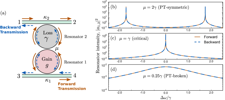
Fig. 1: (a) Schematic of a resonator with saturable gain coupled to a lossy resonator, with both resonators coupled to optical fiber ports. Solid arrows indicate forward transmission (port $1\rightarrow 4$), and dashed arrows indicate backward transmission (port $4\rightarrow 1$). (b)–(d) Transmission characteristics in the linear (non-gain-saturated) regime, when the gain and loss are $PT$ symmetric ($g=\gamma=0.4$). Here, we plot the intensity in the active resonator ($|a_{1}|^{2}$) under forward transmission (solid lines), and in the passive resonator ($|a_{2}|^{2}$) under backward transmission (dashes), versus the frequency detuning. These resonator intensities are proportional to the forward and backward transmission intensities via Eqs. (3) and (6). In the $PT$-symmetric phase $\mu>\gamma$, there are two transmission peaks; in the $PT$-broken phase $\mu<\gamma$, these merge into a single peak.

For backward transmission, a different set of coupled-mode equations holds:

$$\frac{da_{1}}{dt} =(i\Delta\omega_{1}+g)a_{1}-i\mu a_{2}+\sqrt{\kappa_{1}}\,s_{\mathrm{in}}$$ (4)

$$\frac{da_{2}}{dt} =(i\Delta\omega_{2}-\gamma)a_{2}-i\mu a_{1}$$ (5)

$$I_{B} =\kappa_{2}\,|a_{2}|^{2},$$ (6)

where $I_{B}$ is the power transmitted into port 1.

The gain/loss rates $g$ and $\gamma$ consist of several radiative and non-radiative terms [9]:

$$g =\frac{1}{2}\left(g^{\prime}-\gamma_{1}-\kappa_{1}\right)$$ (7)

$$\gamma =\frac{1}{2}\left(\gamma_{2}+\kappa_{2}\right),$$ (8)

where $g^{\prime}$ is the intrinsic amplification rate in resonator 1, and $\gamma_{1,2}$ are the intrinsic loss rates in the resonators. Until stated otherwise, we will impose the following simplifying restrictions:

$$\kappa_{1} =\kappa_{2}=\gamma_{1}=\gamma_{2},$$ (9)

$$\Delta\omega_{1} =\Delta\omega_{2}\equiv\Delta\omega,$$ (10)

$$g^{\prime} =\frac{g_{0}}{1+\left|a_{1}/a_{s}\right|^{2}}.$$ (11)

Equation (9) corresponds to a “critical coupling” criterion with respect to the individual cavity-waveguide couplings. The intrinsic loss and outcoupling rates are all tuned to the same value; note also that $g=g^{\prime}/2-\gamma$. Equation (10) states that the resonators have the same natural frequency. Equations (9)–(10) serve as simplifying assumptions, to avoid dealing with a proliferation of free parameters; later, we will discuss the implications of relaxing these assumptions. Another important constraint, $PT$ symmetry, will be imposed in the next section. Equation (11) describes saturable gain, where $g_{0}$ is the unsaturated amplification rate, and $a_{s}\in\mathbb{R}^{+}$ is a gain saturation threshold.

The experimentally realized systems reported in [9, 10] operated in the 1550 nm wavelength band, with rate parameters $\mu$, $g_{0}$, $\gamma$ and $\kappa_{1,2}$ on the order of 10 MHz in [9], and 100 MHz in [10]. The coupling rates $\mu$ and $\kappa_{1,2}$ can be tuned via the inter-resonator and resonator-waveguide separations. The input power $|s_{\mathrm{in}}|^{2}$ ranged from zero to around 10–100 $\mu$W [9, 10].

The suitability of the system as an optical isolator is characterized using the “isolation ratio”, which is the ratio of forward to backward transmittance at fixed input power:

$$R\equiv\frac{T_{F}}{T_{B}}=\frac{I_{F}(I_{\mathrm{in}})}{I_{B}(I_{\mathrm{in}})},$$ (12)

where $I_{F}$ is obtained by solving Eqs. (1)–(3) with $\dot{a_{1}}=\dot{a_{2}}=0$ (steady state), and $I_{B}$ is obtained from Eqs. (4)–(6). When the system is reciprocal, $R=1$. The isolation ratio was also used in [9, 10] as the figure of merit for optical isolation. However, it is worth noting that the forward and backward transmissions are being compared under the assumption that, in either case, no reflected wave is present. We will discuss this limitation in greater detail in Section 7.

3 Linear operation

We now impose the important constraint $g=\gamma$. This means that in the linear regime, $a_{s}\rightarrow\infty$, the gain and loss resonators become $PT$ symmetric. To understand the implications, consider the “closed” system without resonator-fiber couplings. Its detuning eigenfrequencies are

$$\Delta\omega=i\,\frac{g-\gamma}{2}\pm\sqrt{\mu^{2}-\gamma g-\left(\frac{g-\gamma}{2}\right)^{2}}.$$ (13)

When $g=\gamma$, these reduce to $\Delta\omega=\pm\sqrt{\mu^{2}-\gamma^{2}}$. As $\mu$ and $\gamma$ are varied while keeping $g=\gamma$, the system has a $PT$ symmetry-breaking transition at $\mu=\gamma$. For $\mu>\gamma$, the detunings are real ($PT$-symmetric phase), and for $\mu<\gamma$ they are purely imaginary ($PT$-broken phase).

With the resonator-fiber couplings introduced, the eigenmodes become transmission resonances. In the $PT$-symmetric phase $\mu>\gamma$, the resonator modes and transmission amplitudes exhibit two intensity peaks, at $\Delta\omega=\pm\sqrt{\mu^{2}-\gamma^{2}}$, corresponding to the (real) detunings of the closed system, as shown in Fig. 1(b). In the $PT$-broken phase $\mu<\gamma$, there is a single peak at zero detuning, as shown in Fig. 1(d). As noted by Peng et al. [9], the $PT$-symmetric and $PT$-broken phases will give very different behaviors once gain saturation is introduced.

In the linear regime, Eqs. (1)–(3) and Eqs. (4)–(6) obey optical reciprocity by explicit construction [33]. For fixed $s_{\mathrm{in}}$, the forward and backward transmission amplitudes are exactly equal, $I_{F}=I_{B}$; the isolation ratio is $R=1$, as shown in Fig. 1(b)–(d).

4 Nonlinear operation: multiple solutions and stability

We turn now to the nonlinear, gain-saturated regime, setting $g_{0}=4\gamma$, so that $g\rightarrow\gamma$ as $a_{s}\rightarrow\infty$. This means the system would be $PT$ symmetric in the absence of gain saturation. If we use $a_{s}$ as the natural intensity scale for the coupled-mode equations, the nonlinear system has four remaining independent parameters: $\Delta\omega$, $\mu$, $\gamma$, and $|s_{\mathrm{in}}|^{2}$.

For finite $a_{s}$, optical reciprocity is broken. However, the system is no longer $PT$ symmetric, since $g\neq\gamma$, and thus we can no longer rigorously define “$PT$ symmetric” or “$PT$ broken” phases. Still, we can relate the nonlinear system’s behavior to the $PT$ symmetric phases as defined in the linear limit.

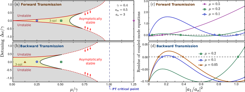
Fig. 2: (a)–(b) Domains in which the nonlinear coupled-mode equations have multiple steady-state solutions, for forward (a) and backward (b) transmission. Here, we show the parameter space defined by the frequency detuning $\Delta\omega$ and inter-resonator coupling $\mu$, with fixed $\gamma=0.4$, $s_{\mathrm{in}}=0.5$, and $a_{s}=3$; symbols indicate the points in the parameter space corresponding to the curves in (c) and (d). Within the small-$\Delta\omega$ region bounded by the red curves, the highest-intensity (or only) solution is asymptotically stable. (c)–(d) Plots showing the emergence of multiple solutions at several values of $\mu$, fixing $\Delta\omega=0$. The horizontal axis is the normalized intensity in the gain resonator, $|a_{1}/a_{s}|^{2}$; the vertical axis is the left-hand side of the cubic Eq. (14), and its counterpart for backward transmission; the steady-state coupled-mode equations are satisfied when the curves cross zero.

In the linear regime, the solutions to the coupled-mode equations were unique. With nonlinearity, the coupled-mode equations can have multiple steady-state solutions. For forward transmission, steady-state solutions are determined by combining Eqs. (1)–(2) into:

$$|\alpha|^{2}x^{3}+\Big{(}2|\alpha-1|^{2}-2-\beta\Big{)}x^{2}+\Big{(}|\alpha-2|^{2}-2\beta\Big{)}x-\beta=0,$$ (14)

where $\alpha$, $\beta$, and $x$ are the following dimensionless variables:

$$\alpha=\frac{(-i\Delta\omega+\gamma)^{2}+\mu^{2}}{\gamma(-i\Delta\omega+\gamma)},\quad\beta=\frac{\mu^{2}}{\Delta\omega^{2}+\gamma^{2}}\,\frac{1}{\gamma}\,\left|\frac{s_{\mathrm{in}}}{a_{s}}\right|^{2},\quad x=\left|\frac{a_{1}}{a_{s}}\right|^{2}.$$ (15)

Since $x\in\mathbb{R}^{+}$, there is either one, two, or three physical steady-state solutions. There must be at least one solution, since the polynomial has a positive third-order coefficient and negative zeroth-order coefficient. The backward transmission case is handled similarly, using Eqs. (4)–(5); it gives the same cubic equation as Eq. (14), but with the replacement

$$\beta=\frac{1}{\gamma}\,\left|\frac{s_{\mathrm{in}}}{a_{s}}\right|^{2}.$$ (16)

Solving the polynomial reveals a domain in parameter space where there are three physical steady-state solutions, outside of which the solution is unique. This is shown in Fig. 2(a)–(b). The three-solution domain lies within the “$PT$-broken” phase of the linear system, $\mu<\gamma$.

The boundaries of the three-solution domain depend on $\gamma$ and $s_{\mathrm{in}}$, as the choice of forward or backward transmission. It consists of two sets of curves; the black curves in Fig. 2(a)–(b) involve a degeneracy of two low-intensity roots of the cubic polynomial [Fig. 2(c)–(d)]. Crossing this boundary causes no discontinuity in the intensity of the stable steady-state solution. The red curves in Fig. 2(a)–(b) involve the degeneracy of two high-intensity roots of the cubic polynomial (14); crossing this boundary destabilizes the steady-state solution.

Through numerical stability analysis, detailed in Appendix A, we find that the highest-intensity solution in the three-solution domain is asymptotically stable (i.e., the Lyapunov exponents are all negative). The two lower-intensity solutions are unstable: small perturbations from these steady states eventually evolve into the highest-intensity state. In the one-solution domain, the solution is asymptotically stable for small detuning $\Delta\omega$, and unstable for large $\Delta\omega$.

Interestingly, the region of asymptotic stability in the nonlinear system is closely connected to the $PT$ symmetry phases of the linear system. For $\mu<\gamma$, which corresponds to the $PT$-broken phase, the frequency range of asymptotic stability is bounded by the solid and dashed red curves shown in Fig. 2(a)–(b). These bounds diverge at $\mu=\gamma$, which corresponds to the transition from the $PT$-broken to the $PT$-symmetric phase in the linear system. For $\mu>\gamma$, the steady state solution becomes asymptotically stable for all $\Delta\omega$.

In the one-solution domain, the onset of asymptotic instability (at sufficiently large $\Delta\omega$) is associated with the appearance of sustained time-domain beating in both the resonator intensities and the transmittance. This is a Hopf bifurcation [36] from a stable state to limit cycle behavior (see Fig. 7 in Appendix A).

5 Isolation ratios at zero detuning

Let us now focus on zero detuning, $\Delta\omega=0$. In this case, there is always an asymptotically stable steady-state solution, and we shall be able to derive an important connection to the $PT$ transition of the linear system. The variables $\alpha$ and $\beta$, defined in Eq. (15), simplify to

$$\alpha =1+\left(\frac{\mu}{\gamma}\right)^{2}$$ (17)

$$\beta =\frac{\left|s_{\mathrm{in}}/a_{s}\right|^{2}}{\gamma}\times\left\{\begin{array}[]{ll}\displaystyle\left(\frac{\mu}{\gamma}\right)^{2},&(\text{Forward})\\ 1,&(\text{Backward}).\end{array}\right.$$ (20)

Hence, the cubic polynomial in Eq. (14) is entirely determined by two quantities: (i) $\mu/\gamma$ and (ii) $|s_{\mathrm{in}}/a_{s}|^{2}/\gamma$. The first quantity is also the tuning parameter for the $PT$ transition. The second quantity determines the strength of the input relative to the gain saturation threshold. We will be particularly interested in the “weak-input” limit, defined as

$$s_{\mathrm{in}}\ll\sqrt{\gamma}\,a_{s}.$$ (21)

When $\beta\ll 1$, the steady state behavior will be principally determined by the $PT$-tuning parameter $\mu/\gamma$.

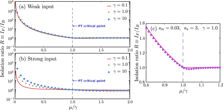
Fig. 3: Isolation ratio versus $\mu/\gamma$ at zero frequency detuning ($\Delta\omega=0$), for (a) weak inputs $s_{\mathrm{in}}=0.15$ and $a_{s}=3$, and (b) strong inputs regime $s_{\mathrm{in}}=9$ and $a_{s}=3$, using several choices of $\gamma$. In the weak-input regime, the isolation ratio is mainly determined by the $PT$-breaking parameter $\mu/\gamma$. The system becomes reciprocal for $\mu/\gamma>1$, corresponding to the $PT$-symmetric phase of the linear system. (c) Close-up of the isolation ratio behavior in the weak-input regime, showing the kink in the dependence on $\mu/\gamma$ at the $PT$ transition point $\mu/\gamma=1$. Circles show exact numerical solutions of the coupled-mode equations, and the solid curve shows the analytic approximations of Eqs. (24)–(25).

Figure 3 plots the isolation ratio $R\equiv I_{F}/I_{B}$ versus $\mu/\gamma$, for several different values of $\gamma$ and $s_{\mathrm{in}}$. In the weak-input regime, the isolation ratio curves are almost identical for different $\gamma$, which verifies that the system is controlled by the combination $\mu/\gamma$. For $\mu/\gamma<1$, corresponding to the $PT$-broken phase of the linear system, we find that $R>1$, and hence the system functions as a good optical isolator. For $\mu/\gamma>1$, we find that $R\approx 1$. This agrees with the qualitative behaviors reported in [9].

Let us examine the vicinity of the transition point in greater detail. Figure 3(c) shows that in the weak input regime, the isolation ratio curve exhibits a kink at $\mu/\gamma=1$. To understand this, we return to the definition of the isolation ratio:

$$R=\frac{I_{F}}{I_{B}}=\left(\mu/\gamma\right)^{-2}\,\frac{x_{F}}{x_{B}},$$ (22)

where $x_{F}$ and $x_{B}$ are the solutions to Eq. (14) for the forward and backward transmission cases. For $\beta\rightarrow 0$, Eq. (14) reduces to

$$x\left(x-\frac{1-(\mu/\gamma)^{2}}{1+(\mu/\gamma)^{2}}\right)^{2}\approx 0.$$ (23)

For $\mu/\gamma<1$, the double-root in Eq. (23) is positive. Hence, in this approximation, the three-solution domain discussed in Section 4 extends over the entire range $\mu/\gamma<1$ along the zero-detuning line. The asymptotically stable solution corresponds to the double-root, which is equal for forward and backward transmission, to lowest order in $\beta$. Hence, we can use Eq. (22) to show that

$$R\approx\left(\mu/\gamma\right)^{-2}\;\;\;\text{for}\;\;\mu/\gamma<1,\;\;s_{\mathrm{in}}\ll\sqrt{\gamma}\,a_{s}.$$ (24)

For $\mu/\gamma>1$, the double-root is negative, so the only valid root in the $\beta\rightarrow 0$ limit is $x=0$. For non-zero $\beta$, this root becomes $\mathcal{O}(\beta)$, so Eq. (20) implies that $x_{F}/x_{B}\approx(\mu/\gamma)^{2}$. This yields the isolation ratio

$$R\approx 1\quad\quad\quad\text{for}\;\;\mu/\gamma>1,\;\;s_{\mathrm{in}}\ll\sqrt{\gamma}\,a_{s}.$$ (25)

The limiting expressions (24)–(25) are plotted in Fig. 3(c), and agree well with the numerical solutions. This helps explain why the $PT$ phase of the linear system affects the isolation functionality of the nonlinear system. Both phenomena are determined by the parameter $\mu/\gamma$, with a critical point at $\mu/\gamma=1$. The kink in the isolation ratio arises from switching solution branches at the critical point.

6 Imbalanced input/output couplings

Thus far, we have assumed that the waveguide-resonator couplings, $\kappa_{1}$ and $\kappa_{2}$, are equal. If the couplings are unequal, the isolation behavior of the system can be quite different. To study this, we replace Eq. (9) with

$$\gamma_{1}+\kappa_{1}=\gamma_{2}+\kappa_{2}=2\gamma.$$ (26)

For $g_{0}=4\gamma$, the gain in resonator 1 is

$$g=\frac{2\gamma}{1+|a_{1}/a_{s}|^{2}}-\gamma,$$ (27)

which ensures that the decoupled system remains $PT$ symmetric with critical point $\mu=\gamma$, as before. With this generalization, the steady-state equations (14)–(16) are altered only by the replacements

$$\begin{aligned} \beta&\rightarrow\frac{\kappa_{2}}{\gamma}\beta\;\;\;(\text{Forward})\\ \beta&\rightarrow\frac{\kappa_{1}}{\gamma}\beta\;\;\;(\text{Backward}).\end{aligned}$$ (28)

By varying the couplings and losses so that Eq. (26) is satisfied, we can access different values of $\kappa_{1}/\kappa_{2}$, subject to the constraint $0<\kappa_{1},\kappa_{2}<2\gamma$.

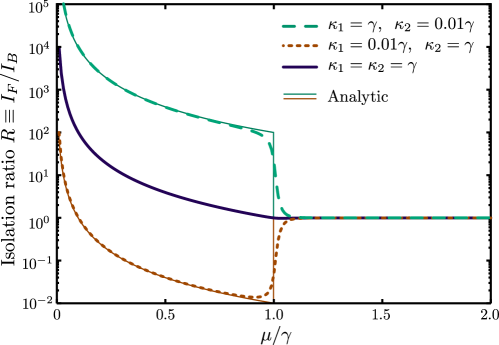
Fig. 4: Isolation ratio versus $\mu/\gamma$ for different microcavity-waveguide coupling rates. The system parameters are $\Delta\omega=0$, $s_{\mathrm{in}}=0.03$, $a_{s}=3$, $\gamma=1$, and $g_{0}=4\gamma$. Thin solid lines show the analytic approximation in the weak-input limit ($s_{\mathrm{in}}\ll\sqrt{\gamma}\,a_{s}$), given by Eq. (29).

The discussion of Section 5 generalizes to this case in a straightforward way. Using the previous zero-detuning and weak-input assumptions, we find that $x_{F}/x_{B}\approx 1$ for $\mu/\gamma<1$, as before; but for $\mu/\gamma>1$, Eq. (28) gives $x_{F}/x_{B}\approx\beta_{F}/\beta_{B}=(\kappa_{2}/\kappa_{1})(\mu/\gamma)^{2}$. The isolation ratio now becomes

$$\begin{aligned} R&=(\kappa_{1}/\kappa_{2})(\mu/\gamma)^{-2}x_{F}/x_{B}\\ &\approx\left\{\begin{array}[]{ll}(\kappa_{1}/\kappa_{2})\,\left(\mu/\gamma\right)^{-2}&\text{for}\;\;\mu/\gamma<1\\ 1&\text{for}\;\;\mu/\gamma>1.\end{array}\right.\end{aligned}$$ (29)

For $\kappa_{1}\neq\kappa_{2}$, this predicts a discontinuity in the isolation ratio at $\mu/\gamma=1$.

Figure 4 plots dependence of the isolation ratios on $\mu/\gamma$, at zero detuning, for the cases of (i) $\kappa_{1}\ll\kappa_{2}$, (ii) $\kappa_{1}\gg\kappa_{2}$, and (iii) $\kappa_{1}=\kappa_{2}$. In all three cases, the isolation ratio approaches unity for $\mu/\gamma>1$. However, for $\mu/\gamma<1$, the unequal-coupling curves exhibit an abrupt change corresponding to a factor of $\kappa_{1}/\kappa_{2}$ (which is two orders of magnitude for these examples). Interestingly, for $\kappa_{1}\ll\kappa_{2}$, the isolation ratio in fact decreases below unity, before increasing again as $\mu/\gamma\rightarrow 0$. The numerical results match Eq. (29) very well.

This phenomenon may be exploited in device applications for realizing an actively switchable optical isolator. Using a small variation in the $\mu/\gamma$ parameter (e.g., by varying the inter-cavity separation, which affects $\mu$), we can switch between strong optically isolating and reciprocal regimes.

7 Effect of a simultaneous reflected wave

We have analyzed the nonlinear system and its isolation ratio under the assumption that light propagates in one direction at a time (i.e., forward or backward). This is a good assumption if the isolator is part of a optical circuit operating with optical pulses, such that any reflected pulse re-entering the isolator (due to scattering from other parts of the circuit) does so at a later time, after the initial pulse has already died away. When forward and backward waves are simultaneously present, however, both contribute to the nonlinearity, causing the isolator to fail. This is a general limitation of optical isolators based on nonlinearity [11].

In order to model simultaneous forward and backward waves, we modify the coupled-mode equations to include resonator modes with the opposite circulation. Similar to the previous “forward” configuration, we suppose the main incident wave enters at port 1 with amplitude $s_{f}$. In addition, there is a back-propagating wave, incident at port 4 with amplitude $s_{b}$, which eventually exits at port 1. The modified equations are (taking $\Delta\omega=0$ for simplicity):

$$\frac{da_{1}}{dt} =ga_{1}-i\mu a_{2}$$ (30)

$$\frac{da_{2}}{dt} =-\gamma a_{2}-i\mu a_{1}+\sqrt{\kappa_{2}}s_{f}$$ (31)

$$\frac{da_{1}^{\prime}}{dt} =ga_{1}^{\prime}-i\mu a_{2}^{\prime}+\sqrt{\kappa_{1}}s_{b}$$ (32)

$$\frac{da_{2}^{\prime}}{dt} =-\gamma a_{2}^{\prime}-i\mu a_{1}^{\prime}.$$ (33)

The opposite-circulation mode amplitudes are denoted by $a_{1}^{\prime}$ and $a_{2}^{\prime}$. The back-propagating wave enters into the final term on the right-hand side of Eq. (32), coupling to the $a_{1}^{\prime}$ mode. Both modes in the gain resonator now contribute to the gain saturation, so

$$g=\frac{2\gamma}{1+\left|a_{1}/a_{s}\right|^{2}+\left|a_{1}^{\prime}/a_{s}\right|^{2}}-\gamma.$$ (34)

Instead of the isolation ratio, we now consider the transmittance of the backward wave:

$$T_{b}=\frac{\kappa_{2}|a_{2}^{\prime}|^{2}}{|s_{b}|^{2}}.$$ (35)

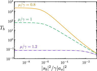
Fig. 5: Transmittance $T_{b}$ of a back-propagating wave, versus the normalized backward incident power $|s_{b}|^{2}/\gamma|a_{s}|^{2}$. A forward-propagating wave with $|s_{f}|^{2}/\gamma|a_{s}|^{2}=10^{-4}$ is simultaneously present; the other parameters are $a_{s}=3$, $\gamma=\kappa_{1}=1$, and $\kappa_{2}=0.01\gamma$. Note that $T_{b}$ can exceed unity because of the presence of gain in the system; this feature can be suppressed if desired by adding loss to the waveguide leads.

Figure 5 plots $T_{b}$ versus the normalized backward incident power , with fixed forward incident power. The features of this plot can be understood as follows: the functioning of the isolator requires the backward wave to cause gain saturation, but when $|s_{b}|^{2}$ is too small, the gain saturation is dominated by the forward wave. Thus, for small $|s_{b}|^{2}$ we find that $T_{b}$ is approximately constant; in fact, it equals the forward transmittance at the power level $|s_{f}|^{2}$. As $|s_{b}|^{2}$ increases, the backward wave starts to affect the gain saturation, and isolation behavior appears in the form of a decrease in $T_{b}$. However, this is only apparent for $\mu<\gamma$ (corresponding to the $PT$-broken regime of the linear system), since it is in this regime that the isolation ratio deviates from unity.

8 Conclusion

We have analyzed the relationship between the linear and nonlinear behaviors of dual microcavity resonators with gain and loss. The $PT$ transition of the linear system is shown to correspond closely with the dynamical and steady-state behaviors of the gain-saturated nonlinear system, for which $PT$ symmetry does not strictly apply. For $\mu>\gamma$, corresponding to the linear system’s “$PT$-symmetric” phase, the resonances are always asymptotically stable, and the isolation ratio approaches unity. But for $\mu<\gamma$, corresponding to the linear system’s “$PT$-broken” phase, the coupled-mode dynamics become unstable at sufficiently large frequency detunings, leading to self-sustained oscillations. If steady-state operation is desired, it is preferable to adopt zero detuning.

Using the “weak-input” approximation, we derived a kink in the isolation ratio at the critical point $\mu=\gamma$. Upon relaxing the constraint of equal waveguide-port couplings, this kink turns into a discontinuity, meaning that the isolation ratios vary extremely quickly with $\mu/\gamma$ in the vicinity of the critical point. This could be useful for using the inter-resonator coupling as an active control parameter. Finally, this analysis assumed that light propagates in one direction at a time, either forward or backwards, which holds for pulsed optical circuits where reflections appear at a later time. If both forward and backward waves are simultaneously present, however, the device will fail to act as a nonlinear isolator if the backward wave is too weak.

Appendix A: Stability analysis

This appendix discusses the stability analysis for the nonlinear coupled-mode equations. For forward transmission, we combine Eqs. (1)–(3) and (9)–(11) with the “$PT$ symmetry” condition $g_{0}=4\gamma$, to obtain the time-dependent equations

$$\frac{da_{1}}{dt} =\left(i\Delta\omega-\frac{\gamma+\kappa_{1}}{2}+\frac{2\gamma}{1+\left|a_{1}/a_{s}\right|^{2}}\right)a_{1}(t)-i\mu a_{2}(t),$$ (36)

$$\frac{da_{2}}{dt} =(i\Delta\omega-\frac{\gamma+\kappa_{2}}{2})\,a_{2}(t)-i\mu a_{1}(t)+\sqrt{\kappa_{2}}\,s_{\mathrm{in}}.$$ (37)

We assume a steady-state input $s_{\mathrm{in}}$, and define

$$a_{1}(t) =\tilde{a_{1}}+\rho_{1}(t)$$ (38)

$$a_{2}(t) =\tilde{a_{2}}+\rho_{2}(t),$$ (39)

where $\tilde{a}_{1,2}$ is the steady-state solution that we wish to analyze and $\rho_{1,2}(t)$ are time-dependent perturbations. We insert this into Eqs. (36)–(37), omitting terms that are quadratic or higher-order in $\rho_{1}$ and $\rho_{2}$. The gain-saturation factor simplifies to:

$$\frac{2\gamma}{1+|a_{s}|^{-2}(\tilde{a}_{1}+\rho_{1})(\tilde{a}_{1}^{*}+\rho_{1}^{*})} \approx\frac{2\gamma}{1+|a_{s}|^{-2}(|\tilde{a}_{1}|^{2}+\tilde{a}_{1}\rho_{1}^{*}+\tilde{a}_{1}^{*}\rho_{1})}$$ (40)

$$\approx\frac{2\gamma}{1+\left|\tilde{a}_{1}/a_{s}\right|^{2}}\,\left[1-\frac{\tilde{a}_{1}\rho_{1}^{*}(t)+\tilde{a_{1}}^{*}\rho_{1}(t)}{|a_{s}|^{2}+|\tilde{a_{1}}|^{2}}\right].$$ (41)

The result is a pair of time-dependent equations,

$$\frac{d\rho_{1}}{dt} =A\rho_{1}(t)+B\rho_{1}^{*}(t)+C\rho_{2}(t)$$ (42)

$$\frac{d\rho_{2}}{dt} =C\rho_{1}(t)+D\rho_{2}(t),$$ (43)

where

$$A =i\Delta\omega\,-\,\frac{\gamma+\kappa_{1}}{2}\,+\,\frac{2\gamma}{1+\left|\tilde{a}_{1}/a_{s}\right|^{2}}\,-\,\frac{2\gamma\,|\tilde{a_{1}}/a_{s}|^{2}}{\left(1+|\tilde{a}_{1}/a_{s}|^{2}\right)^{2}}$$ (44)

$$B =-\frac{2\gamma\,\tilde{a_{1}}^{2}/|a_{s}|^{2}}{\left(1+|\tilde{a}_{1}/a_{s}|^{2}\right)^{2}}$$ (45)

$$C =-i\mu$$ (46)

$$D =i\Delta\omega-\frac{\gamma+\kappa_{2}}{2}$$ (47)

We then assume that the perturbations have the exponential time-dependence

$$\rho_{1}(t) =u_{1}e^{\lambda t}+v_{1}^{*}e^{\lambda^{*}t}$$ (48)

$$\rho_{2}(t) =u_{2}e^{\lambda t}+v_{2}^{*}e^{\lambda^{*}t}.$$ (49)

Plugging these into Eqs. (42)–(47), we derive the matrix equation

$$\begin{bmatrix}A&B&C&0\\ B^{*}&A^{*}&0&C^{*}\\ C&0&D&0\\ 0&C^{*}&0&D^{*}\end{bmatrix}\begin{bmatrix}u_{1}\\ v_{1}\\ u_{2}\\ v_{2}\end{bmatrix}=\lambda\begin{bmatrix}u_{1}\\ v_{1}\\ u_{2}\\ v_{2}\end{bmatrix}.$$ (50)

A stable state must have Lyapunov exponents $\mathrm{Re}(\lambda)<0$ for all four eigenvalues. For backward transmission, we can derive equations that have exactly the same form as Eqs. (42)–(50), except that the steady-state amplitudes $\tilde{a}_{1}$ and $\tilde{a}_{2}$ must be computed using Eqs. (4)–(5).

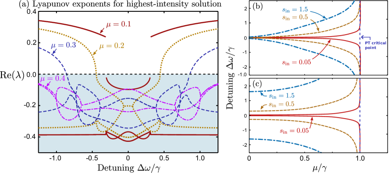
Fig. 6: (a) Lyapunov exponents for the highest-intensity steady-state solution under forward transmission, versus detuning $\Delta\omega$. Results are shown for $\mu\in\{0.1,0.2,0.3,0.4\}$. The other model parameters are fixed at $\gamma=0.4$ and $s_{\mathrm{in}}=0.5$. (b) Bounds of the asymptotic stability region under forward transmission, for several values of the amplitude $s_{\mathrm{in}}$, with fixed $\gamma=0.4$ and $a_{s}=3$. The bandwidth of the asymptotic stability region increases with $\mu$, and diverges at $\mu=\gamma$, which is the $PT$ transition point of the linear system. (c) Bounds of the asymptotic stability region under backward transmission, with the same model parameters.

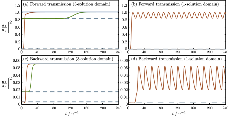
Fig. 7: Time-dependent mode amplitudes under (a) forward transmission for $\Delta\omega=0$ (three-solution domain), (b) forward transmission for $\Delta\omega=0.2$ (one-solution domain), (c) backward transmission for $\Delta\omega=0$ (three-solution domain), and (d) backward transmission for $\Delta\omega=0.2$ (one-solution domain). The other model parameters are $\mu=0.1$, $\gamma=0.4$, $a_{s}=3.0$, and $s_{\mathrm{in}}=0.5$. We start each simulation with initial conditions perturbed from a steady-state solution by $\delta a_{1}=\delta a_{2}=0.001$. In the three-solution domain, perturbing the two lower-intensity solutions causes the system to evolve to the highest-intensity steady-state, which is asymptotically stable.

As discussed in Section 4, there is a domain in parameter space where the coupled-mode equations admit three solutions. The Lyapunov exponents indicate that the highest-intensity solutions are asymptotically stable. Figure 6(a) plots the Lyapunov exponents for the highest-intensity solutions versus the detuning $\Delta\omega$ (in the parts of this plot that lie outside the three-solution domain, the highest-intensity solution is the only one). The exponents become negative within a frequency band centered around $\Delta\omega=0$. This agrees with Fig. 2(a)–(b). The discontinuity in the $\mu=0.1$ curve results from crossing into the three-solution domain, whereupon a new branch of asymptotically stable solutions become the highest-intensity solutions. For $\mu>\gamma$, the solution is asymptotically stable for all $\Delta\omega$. As for the lower-intensity solutions, they are partially unstable, with one or more exponents satisfying $\mathrm{Re}(\lambda)>0$.

To verify these results, we solve the time-domain coupled-mode equations numerically (using the LSODE solver). Figure 7(a) and (c) shows the time-dependent intensities, under forward and backward transmission, within the three-solution domain ($\mu=0.1$ and $\Delta\omega=0.0$, with $a_{s}=3.0$ $s_{\mathrm{in}}=0.5$ as before). Perturbations to the lower-intensities steady states cause the system to evolve into the highest-intensity steady state, as expected from the stability analysis.

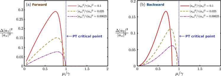
Fig. 8: Beating amplitudes $\Delta|a_{1,2}|^{2}/|a_{s}|^{2}$, defined as the difference of the maximum and minimum values of $|a_{1,2}(t)|^{2}/|a_{s}|^{2}$ over time $t$, versus the $PT$-breaking parameter $\mu/\gamma$. The amplitudes $a_{1,2}(t)$ are solved numerically using the full time-dependent coupled-mode equations, using $\Delta\omega=0.5$, $\gamma=0.4$, $s_{\mathrm{in}}=0.5$, and $a_{s}=3$.

In the single-solution domain, the steady-state solution loses its stability at large detunings, as indicated in Fig. 2(a)–(b). This occurs through a Hopf bifurcation [36]: small perturbations away from the steady state induce a limit cycle, i.e. a self-sustained oscillation in the mode amplitudes, as shown in Fig. 7. The oscillation’s mid-point coincides roughly with the real part of the unphysical complex root of Eq. (14).

Figure 8 shows the beating amplitude versus $\mu/\gamma$. The system is detuned so that $\Delta\omega=0.5$. For small $\mu/\gamma$, the beating is non-zero, but at $\mu\approx\gamma$ the system crosses the asymptotic stability boundary and reaches a steady state where $\Delta|a_{1,2}|^{2}/|a_{s}|^{2}=0$. This is another interesting link between the coupled-mode dynamics and the $PT$ transition.