A Serial Multilevel Hypergraph Partitioning Algorithm

Abstract

The graph partitioning problem has many applications in scientific computing such as computer aided design, data mining, image compression and other applications with sparse-matrix vector multiplications as a kernel operation. In many cases it is advantageous to use hypergraphs as they, compared to graphs, have a more general structure and can be used to model more complex relationships between groups of objects. This motivates our focus on the less-studied hypergraph partitioning problem.

In this paper, we propose a serial multi-level bipartitioning algorithm. One important step in current heuristics for hypergraph partitioning is clustering during which similar vertices must be recognized. This can be particularly difficult in irregular hypergraphs with high variation of vertex degree and hyperedge size; heuristics that rely on local vertex clustering decisions often give poor partitioning quality. A novel feature of the proposed algorithm is to use the techniques of rough set clustering to address this problem. We show that our proposed algorithm gives on average between 18.8% and 71.1% better quality on these irregular hypergraphs by comparing it to state-of-the-art hypergraph partitioning algorithms on benchmarks taken from real applications.

1 Introduction

This paper is concerned with hypergraph partitioning. A hypergraph is a generalization of a graph in which edges (or hyperedges) can contain any number of vertices rather than just two. Thus hypergraphs are able to represent more complex relationships and model less structured data catayk1999 ; hendrickson1998graph ; wang2014bilionnode and thus can, for some applications in High Performance Computing, provide an improved model. For this reason, hypergraph modelling and hypergraph partitioning have become widely used in the analysis of scientific applications alp1996 ; catayk1999 ; curino2010schism ; bey2014 ; hu2014 ; marquez2015 ; tian2009 ; zhou2006learning .

We propose a Feature Extraction Hypergraph Partitioning (FEHG) algorithm for hypergraph partitioning which makes novel use of the technique of rough set clustering. We evaluate it in comparison with several state-of-the-art algorithms.

1.1 The Hypergraph Partitioning Problem

We first define the problem formally. A hypergraph $H=(V,E)$ is a finite set of vertices $V$ and a finite set $E\subseteq 2^{V}$ of hyperedges. Each hyperedge $e\in E$ can contain any number of vertices (constrast with a graph where every edge contains two vertices). Let $e\in E$ and $v\in V$ be a hyperedge and a vertex of $H$, respectively. Then hyperedge $e$ is said to be incident to $v$ or to contain $v$, if $v\in e$. This is denoted $e\triangleright v$. The pair $\langle e,v\rangle$ is further called a pin of $H$. The degree of $v$ is the number of hyperedges incident to $v$ and is denoted $d(v)$. The size or cardinality of a hyperedge $e$ is the number of vertices it contains and is denoted $|e|$. An example of a hypergraph with 16 vertices and 16 hyperedges is given in Fig. 1.

Figure 1: A sample hypergraph $H$ with $16$ vertices and 16 hyperedges. Vertices and hyperedges are represented as square and circular nodes, respectively. The weights of the vertices and hyperedges are assumed to be 1.

Let $\omega\colon V\mapsto\mathbb{N}$ and $\gamma\colon E\mapsto\mathbb{N}$ be functions defined on the vertices and hyperedges of $H$. For $v\in V$ and $e\in E$, we call $\omega(v)$ and $\gamma(e)$ the weights of $v$ and $e$. For a non-negative integer $k$, a k-way partitioning of $H$ is a collection of non-empty disjoint sets $\Pi=\left\{\pi_{1},\pi_{2},\cdots,\pi_{k}\right\}$ such that $\bigcup_{i=1}^{k}\pi_{i}=V$. If $k=2$, we call $\Pi$ a bipartition. We say that vertex $v\in V$ is assigned to a part $\pi$ if $v\in\pi$. Furthermore, the weight of a part $\pi\in\Pi$ is the sum of the weights of the vertices assigned to that part. A hyperedge $e\in E$ is said to be connected to (or spans on) the part $\pi$ if $e\cap\pi\neq\emptyset$. The connectivity degree of a hyperedge $e$ is the number of parts connected to $e$ and is denoted $\lambda_{e}(H,\Pi)$. A hyperedge is said to be cut if its connectivity degree is more than 1.

We define the partitioning cost of a $k$-way partitioning $\Pi$ of a hypergraph $H$:

$$\operatorname{cost}(H,\Pi)=\sum\nolimits_{e\in E}(\gamma(e)\cdot(\lambda_{e}(H,\Pi)-1))$$ (1)

The imbalance tolerance is a real number $\epsilon\in(0,1)$. Then a $k$-way partitioning $\Pi$ of a hypergraph $H$ satisfies the balance constraint if

$$\mkern 1.5mu\overline{\mkern-1.5muW\mkern-1.5mu}\mkern 1.5mu\cdot(1-\epsilon)\leqslant\omega(\pi)\leqslant\mkern 1.5mu\overline{\mkern-1.5muW\mkern-1.5mu}\mkern 1.5mu\cdot(1+\epsilon),\;\forall\pi\in\Pi$$ (2)

where $\mkern 1.5mu\overline{\mkern-1.5muW\mkern-1.5mu}\mkern 1.5mu=\sum\nolimits_{v\in V}\omega(v)/k$ is the average weight of a part.

The Hypergraph Partitioning Problem is to find a $k$-way partitioning with minimum cost subject to the satisfaction of of the balance constraint.

1.2 Heuristics for Hypergraph Partitioning

The Hypergraph Partitioning Problem is known to be NP-Hard garey1979computers , but many good heuristic algorithms have been proposed to solve the problem ccatalyurek2011patoh ; devetal2006 ; fm1982 ; karypis1999kway and we now briefly give an overview of the methods that have been developed.

As graph partitioning is a well-studied problem and good heuristic algorithms are known fjall1998graphsurvey one might expect to solve the hypergraph partitioning problem using graph partitioning. This requires a transformation of the hypergraph into a graph that preserves its structure. There is no known algorithm for this purpose ihler1993 .

Move-based or flat algorithms start with an initialisation step in which vertices are assigned at random to the parts. Then the algorithm builds a new problem solution based on the neighbourhood structure of the hypergraph fm1982 ; san1989kfm . The main weakness of these algorithms is that while the solution found is locally optimal, whether or not it is also globally optimal seems to depend on the density of the hypergraph and the initial random distribution goldberg1983 . Saab and Rao saab1992rao show that the performance of one such algorithm (the KL algorithm) improves as the graph density increases.

Recursive bipartitioning algorithms generate a bipartitioning of the original hypergraph and are then recursively applied independently to both parts until a $k$-way partitioning is obtained fm1982 ; ccatalyurek2011patoh ; devetal2006 . Direct $k$-way algorithms calculate a $k$-way partitioning by working directly on the hypergraph san1989kfm . There is no consensus on which paradigm gives better partitioning. Karypis reports some advantages of direct $k$-way partitioning over recursive algorithms karytech2002 . Cong et al. report that direct algorithms are more likely to get stuck in local minima cong1998 . Aykanat et al. report that direct algorithms give better results for large $k$ aykanat2008fixed . In fact, recursive algorithms are widely used in practice and are seen to achieve good performance and quality.

We mention in passing that other algorithms consider the hypergraph partitioning problem with further restrictions. Multi-constraint algorithms, are used when more than one partitioning objective is defined by assigning a weight vector to the vertices aykanat2008fixed . In the context of VLSI circuit partitioning, there are terminals, such as I/O chips, that are fixed and cannot be moved. Therefore when partitioning these circuits some vertices are fixed and must be assigned to particular parts. Problems of this type are easier to solve and faster running times can be achieved alpert2000fixed ; ccatalyurek2011patoh ; aykanat2008fixed .

In this paper, we introduce a multi-level algorithm so let us describe this general approach. These algorithms have three distinct phases: coarsening, initial partitioning and uncoarsening. During coarsening vertices are merged to obtain hypergraphs with progressively smaller vertex sets. After the coarsening stage, the partitioning problem is solved on the resulting smaller hypergraph. Then in the uncoarsening stage, the coarsening stage is reversed and the solution obtained on the small hypergraph is used to provide a solution on the input hypergraph. The coarsening phase is sometimes also known as the refinement phase.

During coarsening the focus is on finding clusters of vertices to merge to form vertices in the coarser hypergraph. One wishes to merge vertices that are, in some sense, alike so a metric of similarity is required; examples are Euclidean distance, Hyperedge Coarsening, First Choice (FC), or the similarity metrics proposed by Alpert et al. alpert1998multilevel , and Catalyurek and Aykanat catayk1999 .

A problem encountered with high dimensional data sets is that the similarity between objects becomes very non-uniform and defining a similarity measure and finding similar vertices to put into one cluster is very difficult. This situation is more probable when the mean and standard deviation of the vertex degrees increases (see, for example, the analysis of Euclidean distance as a similarity measures by Ertöz et al. ertozetal2003 ). Although other measures, such as cosine measure and jaccard distance, address the issue and resolve the problem to some extent, they also have limitations. For example, Steinbach et al. steinbach2000 have evaluated these measures and found that they fail to capture similarity between text documents in document clustering techniques (used in areas such as text mining and information retrieval). The problem is that cosine and jaccard distances emphasise the importance of shared attributes for measuring similarity and they ignore attributes that are not common to pairs of vertices. Consequently, other algorithms use other clustering techniques to resolve the problem such as shared nearest neighbour (SNN) methods ertoz2002new and global vertex clustering information.

Decisions for vertex clustering are made locally and global decisions are avoided due to their high cost and complexity though they give better results ale2006 . All proposed heuristics reduce the search domain and try to find vertices to be matched using some degree of randomness devetal2006 . This degrades the quality of the partitioning by increasing the possibility of getting stuck in a local minimum and they are highly dependent on the order the vertices are selected for matching. A better trade-off is needed between the low cost of local decisions and the high quality of global ones.

Furthermore, there is a degree of redundancy in modelling scientific applications with hypergraphs. Removing this redundancy can help in some optimisations such as clustering decisions, storage overhead, and processing requirements. An example is proposed by Heinz and Chandra bey2014 in which the hypergraph is transformed into a Hierarchy DAG (HDAG) representation and reducing the memory requirement for storing hypergraphs. Similarly, one can identify redundancies in the coarsening phase and make better vertex clustering decisions and achieve better partitioning on the hypergraph.

The FEHG algorithm proposed in this paper makes novel use of the technique of rough set clustering to categorise the vertices of a hypergraph in the coarsening phase. FEHG treats hyperedges as features of the hypergraph and tries to discard unimportant features to make better clustering decisions. It also focuses on the trade-off to be made between local vertex matching decisions (which have low cost in terms of the space required and time taken) and global decisions (which can be of better quality but have greater costs). The emphasis of our algorithm is on the coarsening phase: good vertex clustering decisions here can lead to high quality partitioning karytech2002 .

2 Preliminaries

2.1 Rough Set Clustering

Rough set clustering is a mathematical approach to uncertainty and vagueness in data analysis. The idea was first introduced by Pawlak in 1991 pawlak1991 . The approach is different from statistical approaches, where the probability distribution of the data is needed, and fuzzy logic, where a degree of membership is required for an object to be a member of a set or cluster. The approach is based on the idea that every object in a universe is tied with some knowledge or attributes such that objects which are tied to the same attributes are indiscernible and can be put together in one category pawlak2005rough .

The data to be classified are called objects and they are described in an information system:

Definition 1 (Information System)

An information system is a system represented as $\mathfrak{I}=(\mathbb{U},\mathbf{A},\mathbf{V},\mathcal{F})$ where: [itemize] @ $\mathbb{U}$ is a non-empty finite set of objects or the universe. @ $\mathbf{A}$ is a non-empty finite set of attributes with size $|\mathbf{A}|=t$. @ $\mathbf{V}=(\mathbf{V}_{1},\mathbf{V}_{2},\ldots,\mathbf{V}_{t})$ where, for each $a\in\mathbf{A}$, $\mathbf{V}_{a}$ is the set of values for $a$. @ $\mathcal{F}:\mathbb{U}\times\mathbf{A}\mapsto\mathbf{V}$ is a mapping function such that, for $u\in\mathbb{U},a\in\mathbf{A}$, $\mathcal{F}(u,a)\in\mathbf{V}_{a}$.

For any subset of attributes $\mathbf{B}=\left\{b_{1},b_{2},\cdots,b_{j}\right\}\subseteq\mathbf{A}$, the B-Indiscernibility relation is defined as follow:

$$\text{IND}(\mathbf{B})=\left\{(u,v)\in\mathbb{U}^{2}\mid\forall b\in\mathbf{B},\,\mathcal{F}(u,b)=\mathcal{F}(v,b)\right\}$$ (3)

When $(u,v)\in\text{IND}(\mathbf{B})$, it is said that $u$ and $v$ are indiscernible under $B$. The equivalence class of $u$ with respect to $B$ is represented as $[u]_{\mathbf{B}}$ and includes all objects which are indiscernible with $u$. The equivalence relation provides a partitioning of the universe $\mathbb{U}$ in which each object belongs only one part and it is denoted $\mathbb{U}/\text{IND}(\mathbf{B})$ or simply $\mathbb{U}/\mathbf{B}$.

The set of attributes can contain some redundancy. Removing this redundancy could lead us to a better clustering decisions and data categorisation while still preserving the indiscernibility relation amongst the objects wroblewski1998 ; ziarko1995 . The remained attributes after removing the redundancy is called the reduct set roughreview2009 . More precisely, if $\mathbf{B}\subseteq\mathbf{A}$, then $\mathbf{B}$ is a reduct of $\mathbf{A}$ if $\mbox{IND}(\mathbf{B})=\mbox{IND}(\mathbf{A})$ and $\mathbf{B}$ is minimal (that is, no attribute can be removed from $\mathbf{B}$ without changing the indiscernibility relation). But the reduct is not unique and it is known that finding a reduct of an information system is an NP-hard problem skowron1992 . This is one of the computational bottlenecks of rough set clustering. A number of heuristic algorithms have been proposed for problems where the number of attributes is small. Examples have been given by Wroblewski using genetic algorithms wroblewski1995 ; wroblewski1998 , and by Ziarko and Shan who use decision tables based on Boolean algebra ziarko1995 . These methods are not applicable to hypergraphs which usually represent applications with high dimensionality and where the operations have to be repeated several time during partitioning. We propose a relaxed feature reduction method for hypergraphs by defining the Hyperedge Connectivity Graph (HCG).

2.2 The Hyperedge Connectivity Graph

The Hyperedge Connectivity Graph (HCG) of a hypergraph is the main tool used used in our algorithm for removing superfluous and redundant information during vertex clustering in the coarsening phase. The similarity between two hyperedges $e_{i}$ and $e_{j}$ is denoted $sim(e_{i}\cdot e_{j})$ (we will discuss later possible similarity measures).

Definition 2 (Hyperedge Connectivity Graph)

For a given similarity threshold $s\in(0,1)$, the Hyperedge Connectivity Graph (HCG) of a hypergraph $H=(V,E)$ is a graph $\mathcal{G}^{s}=(\mathcal{V},\mathcal{E})$ where $\mathcal{V}=E$ and two hyperedges $e_{i},e_{j}\in\mathcal{V}$ are adjacent in $\mathcal{G}^{s}$ if $sim(e_{i},e_{j})\geqslant s$.

The definition is similar to that of intersection graphs erdos1966representation (graphs that represent the intersections of a family of sets) or line graphs of hypergraphs (graphs whose vertex set is the set of the hyperedges of the hypergraph and two hyperedges are adjacent when their intersection is non-empty). The difference is the presence of the similarity measure that reduces the number of edges in the HCG. Different similarity measures, such as Jaccard Index or Cosine Measure, can be used for measuring the similarity. As the hyperedges of the hypergraph are weighted, similarity between two hyperedges is scaled according to the weight of hyperedges: for $e_{i},e_{j}\in E$ the scaling factor is $\frac{\gamma(e_{i})+\gamma(e_{j})}{2\times\max_{e\in E}\left(\gamma(e)\right)}$. One of the characteristics of the HCG is that it assigns hyperedges to non-overlapping clusters (that is, the connected components of the HCG).

3 The Serial Partitioning Algorithm

The proposed Feature Extraction Hypergraph Partitioning (FEHG) algorithm is a multi-level recursive serial bipartitioning algorithm composed of three distinct phases: coarsening, initial partitioning, and uncoarsening. The emphasis of FEHG is on the coarsening phase as it is the most important phase of the multi-level paradigm karytech2002 .

We provide a general outline of the algorithm before going into further detail. In the coarsening phase, we transfer the hypergraph into an information system and we use rough set clustering decisions to match pairs of vertices. This is done in several steps. First, the reduct set is found to reduce the size of the system and remove superfluous information. Second, the vertices of the hypergraph are categorised using their indispensability relations. These categories are denoted as core and non-core where, in some sense, vertices that belong to the same core are good candidates to be matched together and the non-core vertices are what is left over. The cores are traversed before the non-cores for finding pair-vertex matches. The whole coarsening procedure is depicted in Fig. 2.

Figure 2: The coarsening phase at a glance. The dashed arrow means that non-core vertex list is processed after all cores have been processed.

3.1 The Coarsening

The first step of the coarsening stage is to transfer the hypergraph $H=(V,E)$ into an information system. The information system representing the hypergraph is $\mathcal{I}_{H}=(V,E,\mathbf{V},\mathcal{F})$; that is, the objects are the vertices$V$ and the attributes are the hyperedges $E$. We define the set of values as each being in $[0,1]$ and the mapping function is defined as:

$$\mathcal{F}(v,e)=\frac{f(e)}{\sum\nolimits_{\forall e^{\prime}\triangleright v}\gamma(e^{\prime})},$$ (4)

where $f(e)=\gamma(e)$ if $e\triangleright v$ and is otherwise 0.

The transformation of the hypergraph given in Fig. 1 into an information system is given in Table 1.

Table 1: The transformation of the hypergraph $H$ depicted in Fig. 1 into an information system. The values are rounded to 2 decimal places.

	$e_{1}$	$e_{2}$	$e_{3}$	$e_{4}$	$e_{5}$	$e_{6}$	$e_{7}$	$e_{8}$	$e_{9}$	$e_{10}$	$e_{11}$	$e_{12}$	$e_{13}$	$e_{14}$	$e_{15}$	$e_{16}$
$\mathbf{v_{1}}$	$0.33$	$0$	$0$	$0$	$0.33$	$0$	$0$	$0$	$0$	$0.33$	$0$	$0$	$0$	$0$	$0$	$0$
$\mathbf{v_{2}}$	$0.25$	$0.25$	$0$	$0$	$0$	$0$	$0.25$	$0$	$0$	$0$	$0$	$0$	$0$	$0$	$0.25$	$0$
$\mathbf{v_{3}}$	$0$	$0$	$0.33$	$0$	$0$	$0$	$0.33$	$0$	$0.33$	$0$	$0$	$0$	$0$	$0$	$0$	$0$
$\mathbf{v_{4}}$	$0$	$0.16$	$0.16$	$0.16$	$0$	$0$	$0$	$0.16$	$0$	$0$	$0$	$0.16$	$0$	$0$	$0$	$0.16$
$\mathbf{v_{5}}$	$0.33$	$0$	$0$	$0$	$0$	$0$	$0.33$	$0$	$0$	$0.33$	$0$	$0$	$0$	$0$	$0$	$0$
$\mathbf{v_{6}}$	$0$	$0$	$0.33$	$0$	$0$	$0$	$0$	$0$	$0.33$	$0$	$0.33$	$0$	$0$	$0$	$0$	$0$
$\mathbf{v_{7}}$	$0$	$0$	$0$	$0$	$0$	$0.33$	$0.33$	$0$	$0$	$0$	$0$	$0$	$0$	$0.33$	$0$	$0$
$\mathbf{v_{8}}$	$0$	$0.2$	$0$	$0.2$	$0$	$0$	$0$	$0.2$	$0$	$0$	$0$	$0.2$	$0$	$0$	$0$	$0.2$
$\mathbf{v_{9}}$	$0$	$0$	$0$	$0$	$0$	$0.25$	$0$	$0$	$0.25$	$0$	$0.25$	$0$	$0$	$0.25$	$0$	$0$
$\mathbf{v_{10}}$	$0$	$0$	$0$	$0$	$0.33$	$0$	$0$	$0$	$0$	$0.33$	$0$	$0$	$0.33$	$0$	$0$	$0$
$\mathbf{v_{11}}$	$0$	$0$	$0$	$0$	$0$	$0$	$0$	$0$	$0$	$0$	$0.5$	$0$	$0$	$0.5$	$0$	$0$
$\mathbf{v_{12}}$	$0$	$0$	$0$	$0.33$	$0$	$0$	$0$	$0$	$0$	$0$	$0$	$0.33$	$0$	$0$	$0$	$0.33$
$\mathbf{v_{13}}$	$0$	$0$	$0$	$0$	$0.5$	$0$	$0$	$0$	$0$	$0$	$0$	$0$	$0.5$	$0$	$0$	$0$
$\mathbf{v_{14}}$	$0$	$0$	$0$	$0$	$0$	$0$	$0$	$0$	$0$	$0$	$0$	$0$	$0$	$1.0$	$0$	$0$
$\mathbf{v_{15}}$	$0$	$0$	$0$	$0$	$0$	$0$	$0$	$0$	$0$	$0$	$0$	$0$	$0$	$0$	$1.0$	$0$
$\mathbf{v_{16}}$	$0$	$0$	$0$	$0.25$	$0$	$0$	$0$	$0.25$	$0$	$0$	$0$	$0.25$	$0$	$0$	$0$	$0.25$

Calculating the HCG: Initially, hyperedges are not assigned to any cluster. Then, until all hyperedges are assigned, a hyperedge $e$ is selected, a new cluster number is assigned to it and the cluster is developed around $e$ by processing its adjacent hyperedges using Definition 2. At the end of HCG calculation, each hyperedge is assigned to exactly one cluster. We refer to the cluster set as edge partitions and denote it $E^{\mathrm{R}}$. The size and weight of each $e_{\mathrm{R}}\in E^{\mathrm{R}}$ is the number of hyperedges it contains and the sum of their weights, respectively. An example of the HCG for the sample hypergraph in Fig. 1 and similarity threshold $s=0.5$ is depicted in Fig. 3.

Figure 3: An example of Hyperedge Connectivity Graph (HCG) of the hypergraph $H$ depicted in Fig. 1 and the similarity threshold $s=0.5$.

Hyperedges belonging to the same edge partition are considered to be similar. For each edge partition, we choose a representative and all other hyperedges in the same edge partition are removed from the information system $\mathcal{I}_{H}$ and replaced by their representative. After this reduction, the new information system is built and represented as $\mathcal{I}^{\mathrm{R}}_{H}=\left(V,E^{\mathrm{R}},\mathbf{V}^{\mathrm{R}},\mathcal{F}^{\mathrm{R}}\right)$ in which the attribute set is replaced by $E^{\mathrm{R}}$. In the new information system, the set of values is $\mathbf{V}^{\mathrm{R}}_{e_{\mathrm{R}}}\subseteq\mathbb{N}$. Furthermore, the mapping function for $\forall e_{\mathrm{R}}\in E^{\mathrm{R}}$ is redefined as follows:

$$\mathcal{F}^{\mathrm{R}}(v,e_{\mathrm{R}})=\left|{\left\{e\triangleright v\,\wedge\,e\in e_{\mathrm{R}}|e\in E\ \right\}}\right|.$$ (5)

We can further reduce the set of attributes by picking the most important ones. For this purpose, we define a clustering threshold $c\in[0,1]$ and the mapping function is changed according to Eq.(6) below to construct the final information system $\mathcal{I}^{\mathrm{f}}$.

$$\mathcal{F}^{f}(v,e_{\mathrm{R}})=\begin{cases}1,&\mbox{if}\,\frac{\mathcal{F}^{\mathrm{R}}(v,e_{\mathrm{R}})}{\mid\left\{e\triangleright v,\forall e\in E\right\}\mid}\geqslant c\\ 0,&\mbox{otherwise}.\end{cases}$$ (6)

An example of the reduced information system and the final table using the clustering threshold $c=0.5$ for the hypergraph of Fig. 1 is depicted in Table 3. The final table is very sparse compared to the original table. At this point, we use rough set clustering. For every vertex, we calculate its equivalence class. Then, a partitioning $\mathbb{U}/\text{IND}(E^{\mathrm{R}})$ on the vertex set is obtained using the equivalence relations. We refer to parts in $\mathbb{U}/\text{IND}(E^{\mathrm{R}})$ as cores such that each vertex belongs to a unique core. For some of the vertices in the hypergraph, the mapping function gives zero output for all attributes that is $\mathcal{F}^{\mathrm{f}}(v,e_{\mathrm{R}})=0,\,\forall e_{\mathrm{R}}\in E^{\mathrm{R}}$. These vertices are assigned to a list denoted as the non-core vertex list.

Table 2: The reduced information system that is built based on the HCG in Fig. 3.

	$C_{1}$	$C_{2}$	$C_{3}$	$C_{4}$	$C_{5}$	$C_{6}$
$\mathbf{v_{1}}$	$3$	$0$	$0$	$0$	$0$	$0$
$\mathbf{v_{2}}$	$1$	$1$	$1$	$1$	$0$	$0$
$\mathbf{v_{3}}$	$0$	$0$	$1$	$1$	$0$	$2$
$\mathbf{v_{4}}$	$1$	$0$	$3$	$0$	$0$	$0$
$\mathbf{v_{5}}$	$2$	$0$	$0$	$1$	$0$	$0$
$\mathbf{v_{6}}$	$0$	$0$	$0$	$0$	$0$	$3$
$\mathbf{v_{7}}$	$0$	$0$	$0$	$1$	$2$	$0$
$\mathbf{v_{8}}$	$0$	$0$	$3$	$0$	$0$	$0$
$\mathbf{v_{9}}$	$0$	$0$	$0$	$0$	$2$	$2$
$\mathbf{v_{10}}$	$3$	$0$	$0$	$0$	$0$	$0$
$\mathbf{v_{11}}$	$0$	$0$	$0$	$0$	$1$	$1$
$\mathbf{v_{12}}$	$0$	$0$	$3$	$0$	$0$	$0$
$\mathbf{v_{13}}$	$2$	$0$	$0$	$0$	$0$	$0$
$\mathbf{v_{14}}$	$0$	$0$	$0$	$0$	$1$	$0$
$\mathbf{v_{15}}$	$0$	$1$	$0$	$0$	$0$	$0$
$\mathbf{v_{16}}$	$0$	$0$	$1$	$0$	$0$	$0$

Table 3: The final information system for clustering threshold $c=0.5$.

	$C_{1}$	$C_{2}$	$C_{3}$	$C_{4}$	$C_{5}$	$C_{6}$
$\mathbf{v_{1}}$	$1$	$0$	$0$	$0$	$0$	$0$	}43mm[Core 1]
$\mathbf{v_{5}}$	$1$	$0$	$0$	$0$	$0$	$0$
$\mathbf{v_{10}}$	$1$	$0$	$0$	$0$	$0$	$0$
$\mathbf{v_{13}}$	$1$	$0$	$0$	$0$	$0$	$0$
$\mathbf{v_{2}}$	$0$	$0$	$0$	$0$	$0$	$0$
$\mathbf{v_{3}}$	$0$	$0$	$0$	$0$	$0$	$1$	}23mm[Core 2]
$\mathbf{v_{6}}$	$0$	$0$	$0$	$0$	$0$	$1$
$\mathbf{v_{4}}$	$0$	$0$	$1$	$0$	$0$	$0$	}43mm[Core 3]
$\mathbf{v_{8}}$	$0$	$0$	$1$	$0$	$0$	$0$
$\mathbf{v_{12}}$	$0$	$0$	$1$	$0$	$0$	$0$
$\mathbf{v_{16}}$	$0$	$0$	$1$	$0$	$0$	$0$
$\mathbf{v_{9}}$	$0$	$0$	$0$	$0$	$1$	$1$	}23mm[Core 4]
$\mathbf{v_{11}}$	$0$	$0$	$0$	$0$	$1$	$1$
$\mathbf{v_{7}}$	$0$	$0$	$0$	$0$	$1$	$0$	}23mm[Core 5]
$\mathbf{v_{14}}$	$0$	$0$	$0$	$0$	$1$	$0$
$\mathbf{v_{15}}$	$0$	$1$	$0$	$0$	$0$	$0$	}13mm[Core 6]

We observe that cores are built using global clustering information. The final operation is to match pairs of vertices. Cores are visited sequentially one at a time and they are searched locally to find pair matches. Inside each core, a vertex $u$ is selected at random and matched with its “most similar” neighbour. Then the process is repeated with the remaining vertices. These decisions are made with a local measure of similarity. We use the Weighted Jaccard Index that is defined as follows:

$$J\left(u,v\right)=\frac{\sum_{\left\{e\triangleright v\,\wedge\,e\triangleright u\right\}}\gamma\left(e\right)}{\sum_{\left\{e\triangleright v\,\vee\,e\triangleright u\right\}}\gamma(e)},\quad v,u\in V\mbox{, and}\;\forall e\in E.$$ (7)

This is similar to non-weighted jaccard index in PaToH (where it is called Scaled Heavy Connectivity Matching). This captures similarity in high dimensional datasets better than Euclidean based similarity measures. Vertices that do not find any pair matches during core search are transferred into the non-core vertex list (such as $v_{15}$ in Table 2).

One possible problem is that only a small fraction of the hypergraph’s vertices might belong to cores. This can happen, for example, the average vertex degree in the hypergraph is high so there is a large denominator in Eq.(6).

As proposed by Karypis karytech2002 , we define the compression ratio between two levels of coarsening in the multi-level paradigm with $c$ levels as follows:

$$r=\frac{|V_{i}|}{|V_{i+1}|},\forall 0\leqslant i<c$$ (8)

An advantage of the multi-level approach is that it provides a trade-off between quality and speed-up. The more coarsening levels, the better the partitioning quality, but the longer the running time and the greater the memory consumption. On the other hand, with few coarsening levels, we end up with a large hypergraph in which it is not possible to find a good partitioning. Having many coarsening levels will give a very small coarsest hypergraph with perhaps few feasible solutions. This may result in a poor partitioning quality. Karypis karytech2002 provides a tradeoff between quality and levels of partitioning by limiting the compression ratio $r$ to between $1.5$ and $1.8$. In order to satisfy a certain compression ratio, we will visit the non-core vertex list and select vertices randomly. For every selected vertex, the algorithm finds a pair match among its unmatched adjacent vertices in the non-core list.

When pair matches are found, the hypergraph is contracted to build a coarser hypergraph for the next coarsening level. This is done by merging matched vertices. The weight of the coarser vertex is the sum of the weight of two merged vertices and its set of incident hyperedges is the union of the hyperedges incident on each of the merged vertices. After building the coarser hypergraph, we perform two final operations on the hyperedge list. First, hyperedges of unit size are removed as they do not have any impact on the partitioning cut. Second, identical hyperedges (that is, those having the same vertex set) are detected and each set of identical hyperedges is replaced by a single hyperedge whose weight is the sum of the weight of hyperedges in the set. To find identical hyperedges, each hyperedge is hashed to an integer number based on its vertex list. To avoid hash conflicts, the content of the hyperedges are compared if they hash to the same number.

3.2 Initial Partitioning and Refinement

The coarsening phase ends when the number of the vertices in the coarsest hypergraph is less than a threshold (that is $100$ in our algorithm). The size of the coarsest hypergraph is very small compared to the original hypergraph and its partitioning can be calculated quickly. We use a series of algorithms for this purpose. The best partitioning that preserves the balancing constraint is selected and it is projected back to the original hypergraph. The category of algorithms used for this stage are random (randomly assigns vertices to the parts), linear (linearly assigns vertices to the parts starting from a random part), and FM Based (selects a vertex randomly and assigns it to part 1 and all other vertices to part 0; then the FM algorithm is run and the bipartitioning is developed).

Then partitioning algorithms refine the partitioning as the hypergraph is projected back in the uncoarsening phase. Due to the success of the FM algorithm in practice, we use a variation of FM algorithm known as Early-Exit FM (FM-EE) karytech2002 and Boundary FM (BFM) ccatalyurek2011patoh .

4 Evaluations

In this section we provide the evaluation of our algorithm compared to state-of-the-art partitioning algorithms including PHG (the Zoltan hypergraph partitioner) devetal2006 , PaToH ccatalyurek2011patoh and hMetis hmetis15url . PaToH is a serial hypergraph partitioner developed by Çatalyürek and it is claimed to be the fastest multilevel recursive bipartitioning based tool. The earliest and the most popular tool for serial hypergraph partitioning is hMetis developed by Karypis and Kumar; it is specially designed for VLSI circuit partitioning and the algorithms are based on multilevel partitioning schemes and support recursive bisectioning (shmetis and hmetis) and direct $k$-way partitioning (kmetis). Finally, Zoltan data management services for parallel dynamic applications is a toolkit developed at Sandia National Laboratories. The library includes a wide range of tools for problems such as Dynamic Load Balancing, Graph/Hypergraph Colouring, Matrix Operations, Data Migration, Unstructured Communications, Distributed Directories and Graph/Hypergraph Partitioning. It follows a distributed memory model and uses MPI for interprocessor communications. It is available within Trilinos, an open source software project for scientific applications, since version 9.0 trilinosurl .

All of these algorithms are multi-level recursive bipartitioning algorithms and PHG is a parallel hypergraph partitioner while the other two are serial partitioning tools.

For the evaluation, we have selected a number of test hypergraphs from a variety of scientific applications with different specifications. The hypergraphs are obtained from the University of Florida Sparse Matrix Collection sparsecollection2011 . It is a large database of sparse matrices from real applications. Each sparse matrix from the database is treated as the hypergraph incident matrix with the vertices and hyperedges as rows and columns of the matrix, respectively. This is similar to the column-net model proposed in catayk1999 . The weight of each vertex and each hyperedge is assumed to be 1. The list of test data used for our evaluation is in Table 4.

Table 4: Tested hypergraphs for sequential algorithm simulation and their specifications

Hypergraph	Description	Rows	Columns	Non-Zeros	NSCC1
CNR-2000	Small web crawl of Italian CNR domain	325,557	325,557	3,216,152	100,977
AS-22JULY06	Internet routers	22,963	22,963	96,872	1
CELEGANSNEURAL	Neural Network of Nematode C. Elegans	297	297	2,345	57
NETSCIENCE	Co-authorship of scientists in Network Theory	1,589	1,589	5,484	396
PGPGIANTCOMPO	Largest connected component in graph of PGP users	10,680	10,680	48,632	1
GUPTA1	Linear Programming matrix ($A\times A^{T}$)	31,802	31,802	2,164,210	1
MARK3JAC120	Jacobian from MULTIMOD Mark3	54,929	54,929	322,483	1,921
NOTREDAME_WWW	Barabasi’s web page network of nd.edu	325,729	325,729	929,849	231,666
PATENTS_MAIN	Pajek network: mainNBER US Patent Citations	240,547	240,547	560,943	240,547
STD1_JAC3	Chemical process simulation	21,982	21,982	1,455,374	1
COND-MAT-2005	Collaboration network, www.arxiv.org	40,421	40,421	351,382	1,798

• NSCC stands for the Number of Strongly Connected Components.

The simulations are done on a computer with Intel(R) Xeon(R) CPU E5-2650 2.00GHz processor, 8GB of RAM and 40GB of disk space and the operating system running on the system is 32-Bit Ubuntu 12.04 LTS. Furthermore, we set the imbalance tolerance to $2\%$ and the number of parts (the value of $k$) is each of $\left\{2,4,8,16,32\right\}$. The final imbalances achieved by the algorithms are not reported because the balancing requirement was always met.

4.1 Algorithm Parameters

Each of the evaluated tools has different input parameters that can be set by the user. We use default parameters for each tool. All algorithms use a variation of the FM algorithm (FM-EE and BFM) in their refinement phase. PHG uses an agglomerative coarsening algorithm that uses the inner product as the measure of similarity between the vertices devetal2006 . This is also used in hMetis. The default partitioning tool for hMetis is shmetis and the default coarsening scheme is the Hybrid First Choice (HFC) scheme which is a combination of the First Choice (FC) karytech2002 and Greedy First Choice scheme (which is a variation of the FC algorithm in which vertices are grouped and the grouping is biased in favor of faster reduction in the number of the hyperedges in the coarser hypergraph). PaToH is initialised by setting the SBProbType parameter to PATOH_SUGPARAM_DEFAULT. It uses Absorption Clustering using Pins as the default coarsening algorithm (this is an agglomerative vertex clustering scheme). The similarity metric, known as absorption metric, of two vertices $u$ and $v$ is calculated as follows:

$$\sum_{\left\{\forall e\in E\mid u\in e\textit{ and }v\in e\right\}}\frac{1}{|e|-1}.$$ (9)

The algorithm finds the absorption metric for every pin that connects $u$ and the cluster that vertex $v$ is already assigned to. See the manuals of the tools for the full description of the parameters ccatalyurek2011patoh ; karypis1998hmetis ; zoltanurl .

The FEHG algorithm has two parameters that need to be set: the similarity threshold in Definition 2 for building the HCG, and the clustering threshold in Eq.(6). In the rest of this subsection, we look further at these two parameters.

In graph theory, a set of vertices are said, informally, to be clustered if they induce more edges (or hyperedges) than one would expect if the edges had been placed in the graph at random. There are various ways in which one can formally define a clustering coefficient (CC) of either a vertex or a graph, and for hypergraphs various definitions have been proposed gavin2002functional ; klamt2009hypergraphs ; latapy2008basic . We need something a little different as we are interested in the clustering of hyperedges and we want to take account of their weights. Given a hypergraph $H=(V,E)$, we define CC for a hyperedge $e\in E$ as follows:

$$\text{CC}(e)=\begin{cases}\frac{\sum\nolimits_{\left\{e^{\prime}\cap e\neq\emptyset\right\}}\left(\left(\frac{\left|{e\cap e^{\prime}}\right|}{\left|{e}\right|-1}\right)\cdot\gamma(e^{\prime})\right)}{\sum\nolimits_{\left\{v\in e\right\}}\sum\nolimits_{\left\{e^{\prime\prime}\triangleright v\right\}}\gamma(e^{\prime\prime})},\,\forall e^{\prime},e^{\prime\prime}\in E\backslash e,&\mbox{if}\,\left|{e}\right|>1\\ 0,&\mbox{otherwise},\end{cases}$$ (10)

and the CC of $H$ is calculated as the average of CC over all its hyperedges:

$${CC}_{H}=\sum_{e\in E}{\frac{CC(e)}{|E|}}.$$ (11)

During coarsening, each time we proceed to the next coarsening level, the structure of the hypergraph changes and so the value of CC in the coarser hypergraph is different. To recalculate the CC value in each coarsening level could be costly so we are interested in finding a way of updating the CC value without a complete recalculation (possibly sacrificing accuracy in the process). Foudalis et al. foudalis2011social studied the structure of social network graphs and looked at several characteristic metrics including the clustering coefficient. They found that social networks have high CC compared to random networks, and that the CC is negatively correlated to the degree of vertices. Two vertices with low vertex degree are more likely to cluster to each other than two vertices with higher degree. In addition, Bloznelis bloznelis2013 has theoretically investigated random intersection graphs and shown that the CC is inversely related to the average vertex degree in the graph. Based on these results, we update the value of CC from one coarsening level to the next based on the inverse of the average vertex degree. Finally, the similarity threshold is set as the CC of the hypergraph at the beginning of the coarsening phase. In the simulation section, we investigate how our algorithm performs, in terms of partition quality and running time, when the similarity threshold is updated compared to when it is recalculated in each coarsening level.

Figure 4: The variation of bipartitioning cut based on the clustering threshold. Values are normalised with the best cut for each hypergraph.

In order to investigate the impact of the clustering threshold on the quality of the partitioning, we have checked the dependency of the algorithm on the clustering threshold. Figure 4 depicts the quality of the 2-way partitioning of the hypergraphs for variable clustering threshold values. The cut is normalised based on the best partitioning cut for each hypergraph. The average correlation between the cut and the clustering threshold over all hypergraphs is calculated to be $0.2442$ and excluding CNR-2000 is $0.2096$, a very weak correlation. The standard deviation of the changes with respect to the average cut values is also less than $4.2\%$ over all hypergraphs. Therefore, changing the clustering threshold has a very small effect on the partitioning quality. (An exception occurs for the CNR-2000 hypergraph such that the variation of change is very high.) Hyperedges with high CC values are those that are more likely clustered with other hyperedges and those with low CC values do not form any cluster and form edge partitions in HCG of size 1. Consequently, we can remove every edge partition in HCG of unit size and set the value of the clustering threshold to zero in Eq.(6). As an example, edge partitions $C_{2}$ and $C_{4}$ can be removed from the reduced information system in Table 3 without causing any changes in the cores. Using this strategy, the partitioning cut for CNR-2000 is $29.9\%$ better than the best bipartitioning cut reported in Fig. 4 and this is achieved for $c=0.6$.

4.2 Simulations

In the first evaluation, we assume unit weight for both vertices and hyperedges of the hypergraph. In this situation, a partitioning algorithms performs well if it can capture strongly connected components of the hypergraph. A strongly connected component is a group of the vertices that are tightly coupled together. Assuming that the hypergraph represents a graph (by limiting the hyperedge cardinality to two), a strongly connected component is a clique. Because the weight of all hyperedges is 1, the aim of the partitioning algorithm is to take these cliques out of the cut as they are the major cause of increasing the cut; therefore, the vertex connectivity is more important for identifying those cliques. An algorithm that identifies those cliques and merged their vertices to build a coarser vertex is the one that gives better partitioning quality and the clustering algorithm that captures those strongly connected components in the first few levels of coarsening would obtain competitive partitioning qualities.

Table 5: Quality comparison of the algorithms for different part sizes and $2\%$ imbalance tolerance. The values are normalised according to the minimum value for each hypergraph; therefore, the algorithm that gives $1.0$ cut value is considered to be the best. Unit weights are assumed for both vertices and hyperedges.

		Number of Parts
		2		4		8		16		32
		AVE	BEST	AVE	BEST	AVE	BEST	AVE	BEST	AVE	BEST
	FEHG	1.11	1.00	1.02	1.00	1.04	1.01	1.01	1.00	1.01	1.03
AS-22JULY06	PHG	2.90	2.46	1.77	1.56	1.64	1.36	1.43	1.34	1.37	1.32
	hMetis	1.34	1.95	1.19	1.30	1.16	1.18	1.04	1.06	1.09	1.04
	PaToH	1.00	1.43	1.00	1.03	1.00	1.00	1.00	1.00	1.00	1.00
	Min Value	136	93	355	319	629	599	1051	995	1591	1529
	FEHG	1.00	1.00	1.09	1.00	1.10	1.06	1.11	1.08	1.07	1.03
CELEGANSNEURAL	PHG	1.07	1.00	1.04	1.03	1.02	1.00	1.06	1.00	1.00	1.00
	hMetis	1.17	1.21	1.00	1.05	1.00	1.04	1.00	1.02	1.00	1.00
	PaToH	1.01	1.04	1.00	1.06	1.03	1.07	1.03	1.06	1.05	1.05
	Min Value	79	77	195	184	354	342	548	536	773	769
	FEHG	1.37	1.00	1.71	1.07	1.59	1.41	1.53	1.45	1.63	1.51
CNR–2000	PHG	35.88	45.62	12.48	9.17	5.73	4.84	3.54	2.98	2.42	2.02
	hMetis	12.19	18.82	8.24	8.43	5.08	4.71	3.46	3.29	2.66	2.50
	PaToH	1.00	1.71	1.00	1.00	1.00	1.00	1.00	1.00	1.00	1.00
	Min Value	81	45	244	202	569	509	1014	911	1927	1830
	FEHG	1.00	1.00	1.00	1.00	1.00	1.00	1.01	1.02	1.01	1.00
COND–MAT–2005	PHG	1.17	1.17	1.11	1.10	1.05	1.05	1.03	1.03	1.02	1.01
	hMetis	1.05	1.07	1.11	1.12	1.11	1.12	1.11	1.10	1.01	1.01
	PaToH	1.02	1.02	1.03	1.03	1.00	1.00	1.00	1.10	1.00	1.00
	Min Value	2134	2087	5057	4951	8609	8485	12370	12150	16270	16150
	FEHG	0.0	0.0	0.0	0.0	2.00	1.50	1.50	1.00	2.08	1.81
NETSCIENCE*	PHG	0.0	0.0	0.0	0.0	1.50	1.00	1.40	1.00	1.87	1.5
	hMetis	2.0	2.0	5.0	5.0	4.22	3.50	1.75	1.75	1.99	1.87
	PaToH	0.0	0.0	0.0	0.0	1.00	1.00	1.00	1.00	1.00	1.00
	Min Value	0	0	0	0	2	2	8	8	16	16
	FEHG	2.12	1.27	1.00	1.00	1.04	1.00	1.00	1.08	1.00	1.00
PGPGIANTCOMPO	PHG	13.23	1.83	1.44	1.04	1.25	1.04	1.02	1.00	1.08	1.00
	hMetis	9.7	9.61	1.46	1.71	1.04	1.40	1.31	1.40	1.26	1.27
	PaToH	1.00	1.00	1.04	1.27	1.00	1.04	1.02	1.15	1.08	1.06
	Min Value	18	18	242	200	419	400	695	617	956	930
	FEHG	1.00	1.00	1.00	1.00	1.00	1.00	1.00	1.00	1.00	1.00
GUPTA1	PHG	1.58	1.45	1.31	1.24	1.15	1.04	1.07	1.04	1.09	1.05
	hMetis	1.73	1.82	1.61	1.69	1.58	1.64	1.60	1.57	1.51	1.48
	PaToH	1.22	1.17	1.08	1.09	1.04	1.05	1.05	1.07	1.08	1.09
	Min Value	486	462	1466	1384	3077	2893	5342	5134	8965	8519
	FEHG	1.01	1.01	1.02	1.01	1.01	1.00	1.00	1.00	1.06	1.07
MARK3JAC120	PHG	1.00	1.01	1.02	1.02	1.02	1.00	1.00	1.00	1.72	1.78
	hMetis	1.00	1.00	1.00	1.02	1.00	1.00	1.30	1.00	4.20	1.78
	PaToH	1.00	1.02	1.00	1.00	1.00	1.00	1.26	1.20	1.00	1.00
	Min Value	408	400	1229	1202	2856	2835	6317	6245	3142	2944
	FEHG	0	0	1.00	1.00	1.12	1.12	1.09	1.03	1.06	1.07
NOTREDAME*	PHG	4326	4326	158.56	288.69	13.82	16.78	2.09	3.06	1.72	1.78
	hMetis	880	707	67.92	129.92	10.98	12.65	3.36	3.37	2.23	2.30
	Patoh	24	22	1.90	3.31	1.00	1.00	1.00	1.00	1.00	1.00
	Min Value	0	0	27	13	316	259	1577	1484	3142	2944
	FEHG	1.20	1.00	1.03	1.01	1.05	1.03	1.00	1.00	1.00	1.00
PATENTS–MAIN	PHG	12.49	13.19	2.52	2.30	1.79	1.65	1.42	1.38	1.23	1.18
	hMetis	2.38	2.77	1.16	1.24	1.26	1.43	1.26	1.31	1.21	1.22
	PaToH	1.00	1.02	1.00	1.00	1.00	1.00	1.00	1.00	1.01	1.00
	Min Value	643	528	3490	3198	6451	6096	11322	10640	16927	16460
	FEHG	1.01	1.00	1.00	1.03	1.00	1.00	1.00	1.00	1.00	1.00
STD1–JAC3	PHG	1.15	1.08	1.16	1.10	1.18	1.13	1.28	1.35	1.33	1.29
	hMetis	1.05	1.00	1.52	1.03	1.54	1.23	1.70	1.53	1.71	1.51
	Patoh	1.00	1.00	1.08	1.00	1.16	1.14	1.00	1.26	1.30	1.29
	Min Value	1490	1371	3735	3333	7616	6167	13254	11710	22242	21200

• When the minimum cut for the average or best cases are zero, the values shown are actual cut values rather than normalised values.

Each algorithm is run 20 times and its average cut is stated in Table 5 as well as the best cut among all runs. The results in the table are normalised with respect to the minimum value among algorithms. For example, FEHG finds the minimum average cut of 79 for a bipartitioning on the CELEGANSNEURAL hypergraph. PHG, hMetis and PaToH find, respectively, average bipartitioning cuts that are worse by factors of $1.07$, $1.17$, and $1.01$. The results show that FEHG performs very well compared to PHG and hMetis and it is competitive with PaToH; considering the best cut, this is found in 30 (of the 55 cases) by FEHG and in 27 of the cases by PaToH (this includes some ties). As can be seen from the results, all algorithms give similar partitioning cut when the hypergraph has only a few strongly connected components. In this situation, even the local clustering algorithms can capture these strongly connected components and merge their vertices; therefore the differences in partitioning cut for different algorithms that are using different clustering methods (either global or local) is very small.

As the number of strongly connected components increases, it is harder to identify those components especially when the boundaries between them are not clear and they have overlaps. This situation happens in hypergraphs such as Notredame, Patents-Main, and CNR-2000. As shown, FEHG achieves a superior quality improvement compared to Zoltan and hMetis, but PaToH still generates very good partitionings with absorption clustering using pins. One reason that may explain this is that PaToH allows matching between a group of vertices instead of pair-matching. Therefore, the algorithm can merge strongly connected components of vertices in the first few levels of coarsening and remove them from the cut. Though hMetis also allows multiple matches, it seems that the agglomerative clustering strategy of PaToH is much better compared to the hybrid first choice algorithm in hMetis.

The standard deviation (STD) from the average cut is calculated for some of the algorithms and is reported in Table 6. This shows the reliability of the partitioning algorithm when it is used in practical applications. The values are reported as a percentage of STD based on the average partitioning cut for each algorithm. We note, first, that the standard deviation is an increasing function of the number of parts (this is due to the recursive bipartitioning nature of the algorithms which adds to the STD in each recursion), and, second, that the percentage of the STD based on the average cut is decreasing as the number of parts increases (as the average cut increases exponentially when as the number of parts increases, while the increase of the STD is linear). We observe very good reliability for hMetis despite the fact that it gives the worst quality (on average) compared to the others. If we consider bring the average of the cut into the calculation, the least reliability is obtained for hMetis and PHG. Our evaluations recognises FEHG and PHG as the most reliable algorithms compared to others.

Table 6: The percentage of the Standard Deviation (STD) of the cut based on the average partitioning cut for each algorithm with variable number of parts. Unit weights are assumed for both vertices and hyperedges.

		Number of Parts
		2	4	8	16	32
	FEHG	22.4	8.8	3.8	2.8	1.7
AS-22JULY06	PHG	21.8	14.6	7.6	5.8	4.1
	hMetis	0	1.6	1.6	2.1	1.6
	PaToH	2.9	4.5	3.2	3.5	2.7
	FEHG	56.4	31.3	24.8	14	6.9
CNR-2000	PHG	18.9	24.9	17.4	13.3	11.4
	hMetis	7.5	8.1	8.3	6.8	4.5
	PaToH	47.9	79	17.2	15.1	9.2
	FEHG	1.3	1.1	1.0	0.7	0.6
COND_MAT	PHG	1.5	1.5	1	0.9	0.8
	hMetis	0.6	1.3	0.8	0.9	0.8
	PaToH	1.8	3.7	1.1	1.2	1.1
	FEHG	8	23	18	16	18
PGPGIANT	PHG	48	65	45	53	46
	hMetis	3	11	13	24	25
	PaToH	0	0	7	2	5
	FEHG	20	9.5	4.1	2.3	1.9
GUPTA1	PHG	20.1	18.6	8.6	7.5	4.4
	hMetis	1.7	3.1	2.2	2.6	2.1
	PaToH	0	0	1.7	0.3	0.5
	FEHG	1.5	1.4	0.8	1.3	3.9
MARK3JAC	PHG	1	1.2	0.9	0.8	2.0
	hMetis	3.2	1.2	1	2.6	1.6
	PaToH	0	0.9	0.6	3.1	8.5
	FEHG	0	33.2	11.2	6.7	3.6
NOTREDAME	PHG	0	2.9	1.5	1.6	1.4
	hMetis	9.5	3.5	3.1	2.7	1.8
	Patoh	4.1	15.5	8.5	3.3	2
	FEHG	23.2	7.6	4	2.9	2
PATENTS	PHG	16	19.7	15.1	9.8	7.7
	hMetis	2.4	1.7	1.4	1.1	1.1
	PaToH	10.9	4.2	3.4	2	1.8
	FEHG	17.3	6.6	5.6	4.1	2.5
STD1_JAC3	PHG	13.3	8.7	8.3	4.5	2.7
	hMetis	6.7	29.1	17.5	10.3	7.9
	Patoh	8.4	12.6	7.9	6.2	3.3

(a)

(b) No results for hMetis for 16 and 32 parts.

(c)

Figure 5: Comparing the variation of the average cut for different partitioning numbers. The weight of vertices are unit and the weight of hyperedges are their sizes.

(a)

(b)

(c)

Figure 6: (Continued) Comparing the variation of the average cut for different partitioning numbers. The weight of vertices are unit and the weight of hyperedges are their sizes.

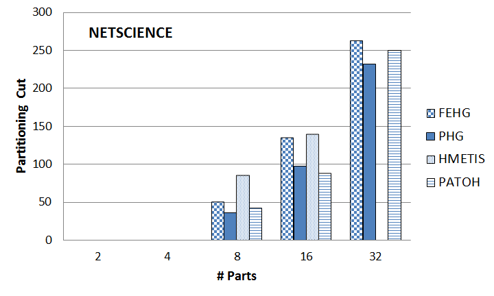
(a) Cut of size zero found for 2-way and 4-way partitioning. No results for hMetis for 32-way partitioning.

(b)

(c)

Figure 7: (Continued) Comparing the variation of the average cut for different partitioning numbers. The weight of vertices are unit and the weight of hyperedges are their sizes.

(a)

(b)

Figure 8: (Continued) Comparing the variation of the average cut for different partitioning numbers. The weight of vertices are unit and the weight of hyperedges are their sizes.

In some practical applications such as parallel distributed systems, hypergraph partitioning is employed to reduce the communication volume between the processor set. In this situation, the weight of hyperedges represents the volume of communications between a group of vertices, and the objective of hypergraph partitioning is to reduce the number of messages communicated between processors as well as the volume of communications. In order to model this scenario, we set the weight of the hyperedges to be their sizes for the next phase of simulations. The main reason for this simulation is that we want to investigate the performance of the clustering algorithms in multi-level hypergraph partitioning tools when there are weights on the hyperedges.

When hyperedges have different weights, vertex connectivity is no longer the only measure used for clustering decisions. Compared to the previous scenario, taking a group of strongly connected components of vertices will not always result in cut reduction as connectivity, as well as how tightly the vertices are connected to each other, is important. The simulation results for this scenario are depicted in Fig. 5.

According to the results, FEHG gives the best partitioning cut on most of the hypergraphs (in 40 out of the 55 cases). In our evaluation, we have three different types of hypergraphs. The first group are those with very irregular structure and high variation of vertex degree or hyperedge size: CNR-2000, GUPTA1, Notredame_WWW, AS-22JULY06, and STD_JAC3. FEHG gives much better quality, finding smaller cuts than the other algorithms in every case. This shows that FEHG suits well this type of hypergraph (such as is found in social networks).

The second group have less irregularity: COND-MAT-2005, PGPGIANTCOMPO, and CELEGANSNEURAL hypergraphs. These hypergraphs have less variable vertex degree or hyperedge size than the first group. Again, FEHG gives the best partitioning results on these types of hypergraphs, but the difference between all partitioners, except hMetis, is small. On these types of hypergraphs, we can get reasonable partitioning quality using local partitioners and the performance of the algorithm highly depends on the vertex similarity measure; for example, the one proposed by hMetis gives the worst quality.

The third group are those with regular structure and very small variability of vertex degree and hyperedge size: NETSCIENCE, PATENTS_MAIN, and MARK3JAC120. The evaluations show that the quality of FEHG is worse than the other partitioners. In the case of NETSCIENCE (which has a very small size), most of the algorithms go through only one level of coarsening. The difference between the cuts is less than 50. Due to the regular structure, local vertex matching decisions give much better results than global vertex matching. We have noticed that in these hypergraphs, the algorithm builds cores that contain a very small fraction of the vertices. Therefore, FEHG mostly relies on the local and random vertex matching which is based on Jaccard similarity. It seems that Jaccard similarity does not perform well compared to the other partitioners and the agglomerative vertex matching of PHG gives the best results.

The results show that PaToH, which was very competitive with our algorithm for the unit hyperedge size tests, here generates very bad partitioning results. This suggests that our algorithm is more reliable than PaToH considered over all types of hypergraphs. Overall, PaToH and, then, hMetis generate the worst partitioning quality. Some of the partitioning results are not reported for hMetis because the algorithm terminates with an internal error on some of the hypergraphs and part numbers. Perhaps the reason is that hMetis suits only partitioning on unit hyperedge size as it is designed for VLSI circuit partitioning.

The running times of the algorithms are reported in Table 7. The ranking of algorithms in order of decreasing running time is hMetis, FEHG, PHG, and PaToH. We note that allowing multiple matches of the vertices can provide not only better partitioning quality compared to pair-matching, but also that it can improve the running time of the algorithm because of the faster reduction in hypergraph size during coarsening. In the case of non-unit hyperedge weights, we have tested our algorithm to see the effects of multiple matching on the performance of the algorithm. In order to do this, we match all vertices that belong to a core when a core is found in our rough set clustering algorithm. The only limitation is that we do not allow the weight of a coarser vertex to exceed the size of a part because it makes it difficult to maintain the balance constraint. The evaluation shows that using multiple matching in our algorithm can improve the runtime by up to 7% and the maximum improvement is observed for CNR-2000 (up to 30% improvement in runtime).

Table 7: Comparing the running time of algorithms for different partitioning. Vertices have unit weights and hyperedge weights are equal to their size. The times are reported in milliseconds.

		Number of Parts
		2	4	8	16	32
	FEHG-ADJ	109	210	308	412	523
AS-22JULY06	PHG	157	274	413	522	634
	hMetis	126	344	803	1370	5902
	PaToH	82	212	336	422	514
	FEHG-ADJ	8	15	21	27	33
CELEGANSNEURAL	PHG	4	7	19	25	22
	HMETIS	12	18	32	–	–
	PATOH	4	4	6	8	12
	FEHG-ADJ	5	10	17	27	34
NETSCIENCE	PHG	4	6	10	22	32
	HMETIS	–	–	14	20	–
	PATOH	2	2	4	4	8
	FEHG-ADJ	114	224	325	408	491
PGPGIANTCOMPO	PHG	44	57	89	114	147
	HMETIS	170	234	354	452	544
	PATOH	12	20	32	46	62
	FEHG-ADJ	19480	30570	39720	50140	57560
CNR-2000	PHG	3035	5202	7317	9267	11060
	HMETIS	22590	41680	50990	61190	68850
	PATOH	2004	3960	6000	8084	10390
	FEHG-ADJ	1843	3014	4020	4918	6095
GUPTA1	PHG	937	1853	2648	3453	4285
	HMETIS	994	4066	11990	43000	331000
	PATOH	914	2140	3544	5370	7298
	FEHG-ADJ	708	1304	1913	2546	3192
MARK3JAC120	PHG	318	588	891	1204	1592
	HMETIS	1748	4570	7010	9410	11130
	PATOH	128	272	416	604	796
	FEHG-ADJ	1588	4071	6487	9095	11130
NOTREDAME_WWW	PHG	2129	3673	5054	6203	7207
	HMETIS	5442	12770	17190	23270	28060
	PATOH	632	1262	1950	2626	3316
	FEHG-ADJ	1933	3187	4430	5860	7514
PATENTS_MAIN	PHG	1274	2156	2919	3610	4251
	HMETIS	11850	24080	32860	38580	42630
	PATOH	396	734	1024	1340	1648
	FEHG-ADJ	4970	12270	19610	26710	32630
STD1_JAC3	PHG	1116	2005	2775	3451	4033
	HMETIS	4086	11480	19610	57300	175500
	PATOH	1720	3884	5372	8380	10830
	FEHG-ADJ	643	1137	1612	2210	2772
COND-MAT-2005	PHG	318	535	750	954	1178
	HMETIS	3800	7038	9930	13740	20020
	PATOH	162	284	370	500	584

In another evaluation, we have evaluated the performance of our clustering coefficient update strategy. For this purpose, we calculate the CC of the hypergraph in every coarsening level and compare the results with when updates are used. The quality does not improve in all cases. For example, the quality of the third type of hypergraph described above was diminished by 1% on average. The best quality improvement is for CNR-2000 that is 6% and it was between 0.2% to 1.5% on other hypergraphs. On the other hand, the runtime of the algorithms are increased by up to 16%. This shows that our update method is very reliable and there is no need to calculate the CC in each coarsening level.

Table 8: The time that FEHG algorithm spends in each phase of the algorithms. Times are reported in seconds.

[90]Parts		[80]AS-22JULY06	[80]CELEGANSNEURAL	[80]NETSCIENCE	[80]PGPGIANTCOMPO	[80]NOTREDAME	[80]PATENTS_MAIN	[80]STD1_JAC3	[80]COND-MAT-2005
	Overall	0.1461	0.0080	0.0059	0.0831	1.5562	1.9312	7.3650	0.6155
	Build	0.0230	0.0003	0.0014	0.0118	0.4568	0.3496	0.4181	0.0697
	Recursion	0.0000	0.0000	0.0000	0.0000	0.0000	0.0000	0.0000	0.0000
2	Vcycle	0.0036	0.0000	0.0003	0.0025	0.0048	0.0604	1.7775	0.0203
	HCG	0.0224	0.0034	0.0007	0.0257	0.0000	0.4512	3.6833	0.2475
	Matching	0.0352	0.0000	0.0009	0.0071	0.0000	0.2275	0.1238	0.0638
	Coarsening	0.0332	0.0000	0.0013	0.0181	0.0000	0.4377	1.1945	0.1108
	InitPart	0.0190	0.0040	0.0003	0.0124	1.0467	0.3019	0.0466	0.0748
	Refinement	0.0086	0.0000	0.0007	0.0051	0.0286	0.0868	0.1072	0.0260
	Overall	0.3722	0.0218	0.0167	0.2456	6.2414	4.9619	18.2084	1.7036
	Build	0.0235	0.0009	0.0006	0.0113	0.5750	0.3474	0.4182	0.0700
	Recursion	0.0161	0.0008	0.0026	0.0081	0.2712	0.2091	0.4072	0.0562
8	Vcycle	0.0095	0.0009	0.0004	0.0088	0.1453	0.1625	4.8115	0.0604
	HCG	0.0514	0.0023	0.0049	0.0727	1.7675	1.1641	8.7172	0.6657
	Matching	0.0903	0.0005	0.0012	0.0184	0.7289	0.5581	0.3300	0.1749
	Coarsening	0.0838	0.0013	0.0043	0.0470	1.3447	1.0932	3.0456	0.3349
	InitPart	0.0650	0.0116	0.0002	0.0553	1.1754	1.1883	0.1084	0.2346
	Refinement	0.0309	0.0033	0.0024	0.0230	0.2041	0.2150	0.3463	0.1017
	Overall	0.6258	0.0360	0.0363	0.4007	9.8867	7.6629	28.5887	2.7925
	Build	0.0233	0.0009	0.0010	0.0110	0.4578	0.3456	0.4173	0.0699
	Recursion	0.0331	0.002	0.0027	0.0157	0.5302	0.3908	0.8082	0.112
32	Vcycle	0.0156	0.0013	0.0024	0.0159	0.2789	0.2547	9.6070	0.0992
	HCG	0.0776	0.0023	0.0029	0.1059	2.9710	1.8239	11.8124	0.9619
	Matching	0.1317	0.0004	0.0028	0.0292	1.1691	0.8517	0.4540	0.2597
	Coarsening	0.1267	0.0012	0.0054	0.0771	2.5044	1.7197	4.3973	0.5536
	InitPart	0.1372	0.0230	0.0133	0.0905	1.4581	1.8681	0.3006	0.4734
	Refinement	0.0772	0.0045	0.0053	0.0535	0.4734	0.3724	0.7559	0.2545

Finally, the detailed running time of FEHG and the amount of time the algorithm spends in each section is given in Table 8 for $\left\{2,8,32\right\}$-way partitioning on some of the hypergraphs. In the table, the overall running time is given in the first row. Build is the time for building data structures and preparation time, recursion is recursive bipartitioning time, vcycle is the amount of time for reduction and hypergraph projection in the multi-level paradigm, HCG is for building HCG, matching includes the time for rough set matching algorithm. Finally, coarsening, initPart and refinement are the time taken for building the coarser hypergraph in the coarsening phase, initial partitioning and uncoarsening phases of FEHG.

The most time consuming part of the algorithm is building HCG: around $27\%$ of the whole running time. The rough set clustering takes only $13\%$ of the runtime. Building the coarser hypergraph and the initial partitioning and the coarsening each takes around $20\%$. One can reduce the initial partitioning time by decreasing the number of algorithms in this section. According to the data, the part where one can most usefully perform optimisations is in building the HCG. If the number of hyperedges is much higher than the number of vertices, its running time can take up most of the algorithm’s running time. The refinement phase takes at most $6\%$ of the whole running time. Therefore, using mores passes of the FM algorithm to improve the quality will not increase the overall time significantly. On the other hand, there is little need for this. As discussed in karytech2002 , a good coarsening algorithm causes less effort in the refinement phase and increasing the passes of the FM algorithm does not make considerable improvement to the cut. This is the case for our FEHG algorithm.

5 Conclusion

In this paper, we have proposed a serial multi-level hypergraph partitioning algorithm (FEHG) based on feature extraction and attribute reduction using rough set clustering. The hypergraph is transformed into an information system and rough set clustering techniques are used to find pair-matches of the vertices during the coarsening phase. This was done by, first, categorising the vertices into core and non-core vertices which is a global clustering decision using indispensability relations. In the later step, cores are traversed one at a time to find best matchings between vertices. This provides a trade-off between global and local vertex matching decisions.

The algorithm is evaluated against the state-of-the-art partitioning algorithms and we have shown that FEHG can achieve up to 40% quality improvement on hypergraphs from real applications. We chose our test hypergraphs to model different scenarios in real applications and we found that FEHG is the most reliable algorithm and generates the highest quality partitionings on most of the hypergraphs. The quality improvement was much better in hypergraphs with more irregular structures; that is, with higher variation of vertex degree or hyperedge size.

We found that one of the drawbacks of local vertex matching decisions is that they perform very differently under various problem circumstances and their behaviour can change based on the structure of the hypergraph under investigation. The worst case observed was PaToH that generated very good and competitive partitioning compared to our algorithm when the hyperedge weights were assumed to be 1, while it gave much worse quality when the hyperedge weights were driven by the hyperedge sizes.

Evaluation of the runtime of the algorithms has shown that the FEHG, while using global clustering decisions, runs slower than PHG and PaToH, but faster than hMetis. We showed that the runtime can be improved by using multiple matching on the vertex set instead of pair-matching. Furthermore, we have observed that the most time consuming part of the algorithm is building HCG. In future work, we are planning to improve this aspect of the proposed algorithm to improve the runtime.

The performance of serial hypergraph partitioning algorithms is limited and it is not possible to partition very large hypergraphs with billions of vertices and hyperedges using the computing resources of one computer, and in future work we will propose a scalable parallel version of the FEHG algorithm based on the parallel rough set clustering techniques.

- (1) Alpert, C., Caldwell, A., Kahng, A., Markov, I.: Hypergraph partitioning with fixed vertices [vlsi cad]. Computer-Aided Design of Integrated Circuits and Systems, IEEE Transactions on 19(2), 267–272 (2000)
- (2) Alpert, C.J.: Multi-way graph and hypergraph partitioning. Ph.D. thesis, UCLA Computer Science Department (1996)
- (3) Alpert, C.J., Huang, J.H., Kahng, A.B.: Multilevel circuit partitioning. Computer-Aided Design of Integrated Circuits and Systems, IEEE Transactions on 17(8), 655–667 (1998)
- (4) Aykanat, C., Cambazoglu, B.B., Uçar, B.: Multi-level direct k-way hypergraph partitioning with multiple constraints and fixed vertices. Journal of Parallel and Distributed Computing 68(5), 609–625 (2008)
- (5) Bloznelis, M., et al.: Degree and clustering coefficient in sparse random intersection graphs. The Annals of Applied Probability 23(3), 1254–1289 (2013)
- (6) Çatalyürek, Ü., Aykanat, C.: Patoh (partitioning tool for hypergraphs). In: Encyclopedia of Parallel Computing, pp. 1479–1487. Springer (2011)
- (7) Catalyurek, U.V., Aykanat, C.: Hypergraph-partitioning-based decomposition for parallel sparse-matrix vector multiplication. Parallel and Distributed Systems, IEEE Transactions on 10(7), 673–693 (1999)
- (8) Cong, J., Lim, S.K.: Multiway partitioning with pairwise movement. In: Proceedings of the 1998 IEEE/ACM International Conference on Computer-aided Design, ICCAD ’98, pp. 512–516. ACM, New York, NY, USA (1998)
- (9) Curino, C., Jones, E., Zhang, Y., Madden, S.: Schism: a workload-driven approach to database replication and partitioning. Proceedings of the VLDB Endowment 3(1-2), 48–57 (2010)
- (10) Davis, T.A., Hu, Y.: The university of florida sparse matrix collection. ACM Transactions on Mathematical Software 38(1), 1 (2011)
- (11) Devine, K., Boman, E., Heaphy, R., Bisseling, R., Catalyurek, U.: Parallel hypergraph partitioning for scientific computing. In: Parallel and Distributed Processing Symposium, 2006. IPDPS 2006. 20th International, p. 10pp (2006)
- (12) Erdos, P., Goodman, A.W., Pósa, L.: The representation of a graph by set intersections. Canad. J. Math 18(106-112), 86 (1966)
- (13) Ertoz, L., Steinbach, M., Kumar, V.: A new shared nearest neighbor clustering algorithm and its applications. In: Workshop on Clustering High Dimensional Data and its Applications at 2nd SIAM International Conference on Data Mining, pp. 105–115 (2002)
- (14) Ertöz, L., Steinbach, M., Kumar, V.: Finding clusters of different sizes, shapes, and densities in noisy, high dimensional data. In: SDM, pp. 47–58. SIAM (2003)
- (15) Fiduccia, C.M., Mattheyses, R.M.: A linear-time heuristic for improving network partitions. In: 19th Conference on Design Automation, pp. 175–181. IEEE (1982)
- (16) Fjällström, P.O.: Algorithms for graph partitioning: A survey. Linköping electronic articles in computer and information science 3(10) (1998)
- (17) Foudalis, I., Jain, K., Papadimitriou, C., Sideri, M.: Modeling social networks through user background and behavior. In: Proceedings of the 8th International Conference on Algorithms and Models for the Web Graph, WAW’11, pp. 85–102. Springer-Verlag (2011)
- (18) Garey, M.R., Johnson, D.S.: Computers and intractability: a guide to the theory of np-completeness. 1979. San Francisco, LA: Freeman (1979)
- (19) Gavin, A.C., Bösche, M., Krause, R., Grandi, P., Marzioch, M., Bauer, A., Schultz, J., Rick, J.M., Michon, A.M., Cruciat, C.M., et al.: Functional organization of the yeast proteome by systematic analysis of protein complexes. Nature 415(6868), 141–147 (2002)
- (20) George, K.: Multilevel hypergraph partitioning. Tech. rep., University of Minnesota (2002)
- (21) Goldberg, M.K., Burstein, M.: Heuristic improvement technique for bisection of VLSI networks. IBM Thomas J. Watson Research Division (1983)
- (22) Heintz, B., Chandra, A.: Beyond graphs: Toward scalable hypergraph analysis systems. SIGMETRICS Perform. Eval. Rev. 41(4), 94–97 (2014)
- (23) Hendrickson, B.: Graph partitioning and parallel solvers: Has the emperor no clothes? In: Solving Irregularly Structured Problems in Parallel, pp. 218–225. Springer (1998)
- (24) Hu, T., Liu, C., Tang, Y., Sun, J., Xiong, H., Sung, S.Y.: High-dimensional clustering: a clique-based hypergraph partitioning framework. Knowledge and information systems 39(1), 61–88 (2014)
- (25) Ihler, E., Wagner, D., Wagner, F.: Modeling hypergraphs by graphs with the same mincut properties. Inf. Process. Lett. 45(4), 171–175 (1993)
- (26) Karypis, G.: hmetis: Hypergraph and circuit partitioning - version 1.5 (2007)
- (27) Karypis, G., Kumar, V.: hmetis: A hypergraph partitioning package version 1.5”, user manual (1998)
- (28) Karypis, G., Kumar, V.: Multilevel k-way hypergraph partitioning. In: Proceedings of ACM/IEEE Design Automation Conference, pp. 343–348 (1999)
- (29) Klamt, S., Haus, U.U., Theis, F.: Hypergraphs and cellular networks. PLoS Comput Biol 5(5), e1000,385 (2009)
- (30) Latapy, M., Magnien, C., Del Vecchio, N.: Basic notions for the analysis of large two-mode networks. Social Networks 30(1), 31–48 (2008)
- (31) Malewicz, G., Austern, M.H., Bik, A.J., Dehnert, J.C., Horn, I., Leiser, N., Czajkowski, G.: Pregel: A system for large-scale graph processing. In: Proceedings of the 2010 ACM SIGMOD International Conference on Management of Data, SIGMOD ’10, pp. 135–146. ACM, New York, NY, USA (2010)
- (32) Márquez, C., Cesar, E., Sorribes, J.: Graph-based automatic dynamic load balancing for hpc agent-based simulations. In Proc. of 3rd Workshop on Parallel and Distributed Agent-Based Simulations (PADABS2015), Vienna, Austria (2015)
- (33) Pawlak, Z.: Rough Sets: Theoretical Aspects of Reasoning About Data. Kluwer Academic Publishers, Norwell, MA, USA (1991)
- (34) Pawlak, Z., Polkowski, L., Skowron, A.: Rough sets: An approach to vagueness. Encyclopedia of Database Technologies and Applications pp. 575–580 (2005)
- (35) Saab, Y., Rao, V.: On the graph bisection problem. Circuits and Systems I: Fundamental Theory and Applications, IEEE Transactions on 39(9), 760–762 (1992)
- (36) Sanchis, L.: Multiple-way network partitioning. Computers, IEEE Transactions on 38(1), 62–81 (1989)
- (37) Sandia National Laboratories: Trilinos: Open source software libraries for the development of scientific applications (2014)
- (38) Sandia National Laboratories: Zoltan: Parallel partitioning, load balancing and data-management services (2014)
- (39) Skowron, A., Rauszer, C.: The discernibility matrices and functions in information systems. In: Intelligent Decision Support, pp. 331–362. Springer (1992)
- (40) Steinbach, M., Karypis, G., Kumar, V., et al.: A comparison of document clustering techniques. KDD workshop on text mining 400(1), 525–526 (2000)
- (41) Thangavel, K., Pethalakshmi, A.: Review: Dimensionality reduction based on rough set theory: A review. Appl. Soft Comput. 9(1), 1–12 (2009)
- (42) Tian, Z., Hwang, T., Kuang, R.: A hypergraph-based learning algorithm for classifying gene expression and arraycgh data with prior knowledge. Bioinformatics 25(21), 2831–2838 (2009)
- (43) Trifunovic, A.: Parallel algorithms for hypergraph partitioning. Ph.D. thesis, University of London (2006)
- (44) Wang, L., Xiao, Y., Shao, B., Wang, H.: How to partition a billion-node graph. In: Data Engineering (ICDE), 2014 IEEE 30th International Conference on, pp. 568–579. IEEE (2014)
- (45) Wróblewski, J.: Finding minimal reducts using genetic algorithms. In: Proccedings of the second annual join conference on infromation science, pp. 186–189 (1995)
- (46) Wróblewski, J.: Genetic algorithms in decomposition and classification problems. In: Rough Sets in Knowledge Discovery 2, pp. 471–487. Springer (1998)
- (47) Zhou, D., Huang, J., Schölkopf, B.: Learning with hypergraphs: Clustering, classification, and embedding. In: Advances in neural information processing systems, pp. 1601–1608 (2006)
- (48) Ziarko, W., Shan, N.: Discovering attribute relationships, dependencies and rules by using rough sets. In: hicss, p. 293. IEEE (1995)