Comment on an Effect Proposed by A.G. Lebed in Semiclassical Gravity

Abstract

A.G. Lebed has given an argument that when a hydrogen atom is transported slowly to a different gravitational potential, it has a certain probability of emitting a photon. He proposes a space-based experiment to detect this effect. I show here that his arguments also imply the existence of nuclear excitations, as well as an effect due to the earth’s motion in the sun’s potential. This is not consistent with previous results from underground radiation detectors. It is also in conflict with astronomical observations.

I Introduction

A.G. Lebedlebed has calculated the behavior of a hydrogen atom that is prepared in its ground state and then transported slowly through the earth’s gravitational field. The metric is taken to be

$$ds^{2}=(1+2\phi)dt^{2}-(1-2\phi)d\ell^{2},$$ (1)

where $c=1$, the spatial line element is $d\ell^{2}=dx^{2}+dy^{2}+dz^{2}$, and the gravitational potential $\phi\ll 1$ varies between the initial and final positions. In ref. lebed , the metrical dilation is treated as an adiabatic perturbation of the Hamiltonian. This perturbation puts the atom into a superposition of states, leading to decay by photon emission with probability $P$.

The more standard approach in semiclassical gravitywald would have been to rewrite the Einstein field equations $G_{ij}=8\pi T_{ij}$ as $G_{ij}=\langle 8\pi T_{ij}\rangle$. In that approach, any excitation of the atom by gravity would result from the curvature of spacetime, which depends on the second derivatives of the metric. In order to calculate the curvature we would need to know not just a parametrization of the form (1) but more detailed information about how the metric varied in a neighborhood of the atom’s world-line. But the phenomenon predicted in ref. lebed   is not a curvature effect. It is an effect of the metric itself (not its derivatives) on an arbitrarily small particle. Furthermore, in the adiabatic approximation the excitation probability $P$ depends only on the value of the metric tensor at the final position as compared with its initial value. Such a comparison is coordinate-dependent, and is presumably meant to be carried out in harmonic coordinates. To a local observer, the emission of radiation would appear to violate conservation of energy; this would have to be accounted for somehow by the extraction of energy from the gravitational field.

Generalizing to systems bound by forces other than electromagnetic ones, let the potential be $U=-kr^{n}$. This allows us to recover the case of an electrical attraction when $k=e^{2}$ and $n=-1$, but we can also mock up a bag of quarks by taking $n=1$. Carrying through the calculations of ref. lebed   with these generalizations, we obtain a perturbation to the Hamiltonian

$$\Delta H=(m+K+U)\phi+V\phi,$$ (2)

where the factor in parentheses is subsumed in the particle’s mass, and the second term contains the operator $V=2K-nU$, which has a vanishing expectation value by the quantum virial theorem.carlip The probability of excitation is the product of two factors, which I notate as

$$P=f_{g}^{2}f_{s}^{2}.$$ (3)

The first of these is gravitational,

$$f_{g}=\phi-\phi_{0}.$$ (4)

The second one depends on the structure of the quantum-mechanical system, and is given by

$$f_{s}=\langle 2|V|1\rangle/\Delta E,$$ (5)

where $\Delta E=E_{2}-E_{1}$ is the difference in energy between the two states. The factor $f_{s}$ is of order unity for hydrogen.lebed

II Solar Effect

We should have effects not just from the earth’s gravity but from the sun’s as well. Moving an atom between the earth’s surface and a distant point, as originally proposed, produces $f_{g}=6.9\times 10^{-10}$. The earth’s motion from perihelion to aphelion gives $f_{g}=3.3\times 10^{-10}$. Since these are within a factor of 2 of one another, it would seem that given any space-based experimental design, one could achieve a far greater sensitivity at a much lower cost by substituting a large sample of atoms on earth for a small sample aboard a space probe.

III Scale-Independence, and Some Systems of Interest

The only dependence of the predicted effect on the structure of the system comes from the value of the exponent $n$ in the potential, and from equation (5) for the quantity $f_{s}$. The latter is the dimensionless ratio of two energies, and does not depend on the linear dimensions of the system, so that the effect is completely independent of scale. This scale-independence arises because the effect is due to the gravitational potential at a point, rather than to curvature. We therefore expect generically that excitations would occur for almost any quantum-mechanical system, including hadrons, nuclei, atoms, and molecules of all sizes.

The structure factor $f_{s}$ depends on the matrix element $V_{21}=\langle 2|V|1\rangle$, and calculating this matrix element explicitly for all of these systems would be a significant project. But regardless of the value of the exponent $n$ in the potential, $V_{21}$ is essentially a measure of the total internal energy of the system, so it is not unreasonable, for the sake of some order-of-magnitude estimates, to assume that it can be estimated as such. There is a selection rule that there can be no change in spin or parity. We would also like to find states 1 and 2 such that 2 has the dynamical character of a radial excitation of 1 so that there is a significant coupling to the metrical dilation measured by $V$, and so that a many-body system can be treated by taking $r$ to be a generalized coordinate describing a collective spatial dilation. Under these assumptions we have simply $f_{s}\sim E/\Delta E$. This ratio will often be of order unity, as in hydrogen, but in some cases it is orders of magnitude higher.

	system	excitation	$E/\Delta E$	radiation
i	proton	$\text{N}(1440)\text{P}_{11}$	$\sim 1$	$\pi^{0}$
ii	heavy nucleus	isoscalar giant monopole resonance	$\sim 10^{2}\text{--}10^{4}$	particle emission
iii	H atom	$n=2$	$\sim 1$	photon
iv	$\text{C}_{60}$ (fullerene)	$0.061\ \text{eV}$ “breathing” mode	$\sim 10^{6}$	photon

Table 1: Properties of some relevant quantum-mechanical systems.

Table 1 summarizes some systems in which one would expect the effect to occur. These are labeled i through iv for reference. The excitations in systems i, ii, and iv have all been interpreted as “breathing” modes of vibration, which suggests that the estimate $f_{s}\sim E/\Delta E$ is reasonable for them.

For an atomic or molecular experiment of the type suggested in ref. lebed , it is to be remarked that rather than hydrogen, other systems, such as large molecules, iv, would be expected to produce excitations with probabilities greater by a factor of $f_{s}^{2}=10^{12}$ or more. Molecules of this size have been diffracted by a grating in experiments, which demonstrates the possibility of placing them in a superposition of states.arndt

The transition rate for example ii is not straightforward to estimate by the techniques used here, but it raises the possibility that otherwise stable nuclei on earth would decay by particle emission.

IV Memory Effect

In the simple example of constant-velocity motion through a uniform gravitational field, the effect is predicted to grow quadratically with the time since the system was first formed. Such a non-exponential decay means that a hydrogen atom, for example, would retain a memory of the potential in which it was formed, and that an observer could access this memory, at least at the statistical level.

Although ref. lebed  proposes using a “tank of a pressurized hydrogen” aboard a satellite, it seems likely that a collision would erase a hydrogen molecule’s memory. It would therefore be preferable to work with a system such as a nucleus, which may remain isolated from its environment for billions of years.

V Hadronic Excitations

In the remainder of this paper I will consider excitation of the proton, example i in table 1. There is an excited state, labeled $\text{N}(1440)\text{P}_{11}$, that matches the spin-parity $1/2^{+}$ of the ground state and is believed to be a radial excitation of the three quarks. For these reasons, we expect $f_{s}\sim E/\Delta E\sim 1$ for excitation of this state. Its most frequent mode of decay is radiation of a neutral pion.

Let us estimate the rate at which hydrogen nuclei on earth would be expected to emit pions. The rate of decay is

$$\Gamma =dP/dt$$ (6)

$$=f_{s}^{2}d(f_{g}^{2})/dt$$ (7)

$$=2f_{s}^{2}(\phi-\phi_{0})d\phi/dt$$ (8)

$$=-2f_{s}^{2}(\phi-\phi_{0})\textbf{g}\cdot\textbf{v},$$ (9)

where g is the sun’s gravitational field and v is the velocity of a hydrogen atom, both as measured by a static observer. (The dependence of the effect on g violates the equivalence principle, and ref. lebed  explicitly interprets the effect as such a violation.)

The potential $\phi_{0}$ would be the potential at which the proton was formed, and we need to define this time of formation. As discussed in section IV, a memory of this potential is carried by the system in this theory, and it is not entirely obvious what would serve to erase its memory. I will assume that this occurs when there is any collision, i.e., when the proton approaches another nucleus, coming within the range of the strong nuclear force. Some protons on earth were formed during big-bang nucleosynthesis (BBN), but others have participated in collisions at the cores of stars. Still others will have undergone their last collision during a type I supernova, near the surface of a white dwarf star. It is a consequence of the model in ref. lebed  that all these classes of protons differ in their subsequent behavior. Since ref. lebed  assumes a static spacetime, we will not consider the BBN component, which has existed over cosmological timescales. For the component whose memory was reset by collisions at the core of a star, we estimate $|\phi_{0,c}|\sim 3M_{\odot}/R_{\odot}\sim 6\times 10^{-6}$, which is $\ll 1$ as assumed in ref. lebed , but much larger than the changes in potential considered there. For those that have been recycled through a supernova, we may have $|\phi_{0,sn}|\sim 10^{-4}$, but the astrophysics is more complicated in this case, so in the following discussion I will use the more conservative estimate based on $\phi_{0,c}$. (Variations in the gravitational potential within the galaxy are smaller than these values, with the potential experienced by our solar system being about $-1.7\times 10^{-6}$.kafle ) In section VI.2, I give an astronomical check on the predictions of ref. lebed  that is entirely independent of such estimates of $\phi_{0}$, or of the assumption that the memory of $\phi_{0}$ can be retained for long periods of time.

Due to the sign of $\phi-\phi_{0}$, these protons would radiate during the half of the year when the earth is moving from perihelion to aphelion. The probability of decay during such a six-month period is estimated to be $7\times 10^{-15}$, resulting in an average rate of radiation

$$\Gamma\sim 4\times 10^{-22}\ \textup{s}^{-1}.$$ (10)

In the following section I will compare this with experiment.

VI Empirical Bounds

VI.1 Underground Radiation Detectors

The excited state of the proton described above decays by emission of a pion, which would be detectable by its decay into a high-energy electromagnetic cascade. A number of underground experiments have already been carried out to detect neutrinos or search for dark matter, and these experiments would have been extremely sensitive to such a phenomenon. One of the most important sources of background in such an experiment is cosmic-ray-induced muons, which also create high-energy cascades. This is the reason that the experiments are carried out underground. In addition, various steps are taken in order to block or reject the resulting events, including the rejection of the kind of high-multiplicity, high-energy events that are of interest here. However, preliminary studies have been carried out in which the experimental trigger was left wide open, in order to precisely characterize the muon-induced background.

I consider here the Large-Volume Detector apparatus (LVD), which consists of 983 tons of hydrocarbon scintillator located about one kilometer underneath the Gran Sasso massif. This scintillator contains $N=9.4\times 10^{31}$ hydrogen atoms. Multiplying by the rate of radiation estimated in section V, we find a predicted count rate

$$R=\Gamma N\sim 2\times 10^{10}\ \textup{s}^{-1}.$$ (11)

The LVD collaboration has made detailed measurements of the flux of muons through their detector.aglietta aglietta2 In these observations, the direction from which the muon entered the detector is reconstructed, and is found to decay exponentially with the depth of rock through which the muon would have had to travel. For angles very close to horizontal, the flux of muons is measured to be $\sim 10^{-12}\ \textup{cm}^{-2}\textup{s}^{-1}\textup{sr}^{-1}$.

The effect discussed here would have caused the creation of similar high-energy electromagnetic cascades originating from protons within the detector’s own active volume. These cascades would have been emitted isotropically, and therefore would have shown up as part of the same count rate attributed above to muon-induced cascades. To be consistent with the measurement above, their rate would have been limited to

$$R\lesssim 3\times 10^{-5}\ \textup{s}^{-1}.$$ (12)

This is inconsistent with expectations from ref. lebed  by a factor of $10^{15}$. Even this is likely to be an underestimate; references aglietta and aglietta2 do not state explicitly whether the analysis looked for such events coming in the upward direction, but if so, then the effect implied by ref. lebed  would be ruled out by even more orders of magnitude.

The Super-Kamiokande collaboration has searched for proton decayskamiokande via the processes $\textup{p}\rightarrow\textup{e}^{+}\pi^{0}$ and $\textup{p}\rightarrow\mu^{+}\pi^{0}$, finding a limit on the rate of decay of $\sim 10^{-41}\ \textup{s}^{-1}$. Since the analysis of the data from this experiment employed sophisticated kinematic reconstructions in order to search for these specific processes, this rate cannot be directly compared with the estimate in equation (10) for the rate of $\textup{p}\rightarrow\textup{p}\pi^{0}$, which would have shown up in the analysis as an event that violated conservation of energy-momentum. Nevertheless, since the two rates differ by a factor of $10^{20}$, it appears unlikely that a background due to neutral pion emission would have gone unnoticed.

VI.2 The Galactic Center

An independent empirical check on the predicted effect comes from observations of stars and gas clouds in tight orbits about Sagittarius A*, the supermassive black hole at the center of our galaxy. Because the potentials experienced by these objects are much larger than the value of $\phi_{0,c}$ assumed above, the behavior of the protons in this environment is independent of the assumption employed earlier that a proton retains a memory of the gravitational potential over billions of years.

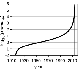
Figure 1: Simulation of the instantaneous power liberated by pion emission in the gas cloud G2, from apastron to periastron. $M=2M_{\odot}$, $\phi_{0}=0$, and $f_{s}=1$ are assumed.

The object G2 is in a highly elliptical, high-velocity orbit about Sag A*. It has been interpreted as a cloud of gas and dust which is heated by a star hidden at its center.witzel Its orbit,gillessen2 with an eccentricity of 0.966, is nearly a radial free-fall toward A*, with periastron taking place in 2013. Its motion and magnitude in the Ks band ($2.2\ \mu\textup{m}$) were observed from 2005 to 2014, and its brightness remained constant throughout this period ($\lesssim 0.2$ magnitudes of variation). A fit to a blackbody curve gives a luminosity of $29L_{\odot}$. If the central star is on the main sequence, then its mass is $2M_{\odot}$; if not, then the mass may be smaller. Figure 1 shows the rate at which energy would have been liberated through pion emission by a body of mass $2M_{\odot}$, composed of hydrogen, tracing out G2’s Keplerian orbit. The result is a spike in power equivalent to $10^{6}L_{\odot}$, which is not consistent with the observed lack of variation, and indeed probably would have destroyed the star. The peak power is not appreciably changed by changing the potential of formation from zero to $\phi_{0}=-8\times 10^{-6}$, which is a typical potential experienced by G2 during its orbit. Therefore this conclusion remains valid even if a proton’s memory of its potential of formation is limited to decades rather than billions of years.

Another astronomical test is available from observations of the star S2, a main-sequence B1 star that is also orbiting Sag A*. Assuming $M=15M_{\odot}$, $\phi_{0}=0$, and $f_{s}=1$, a calculation similar to the one described above gives a peak power of $2\times 10^{7}L_{\odot}$, or about 700 times the normal luminosity of a B1V star. Intriguingly, observations have shown an unexpected 40% rise in the star’s luminosity when it was near perihelion, but explanations have been suggested using standard physics.gillessen

VII Conclusions

I have examined a provocative claim by A.G. Lebed that a quantum-mechanical system can be induced to emit radiation by moving it slowly to a different gravitational potential. This prediction is incompatible with existing terrestrial experiments and astronomical observations.

VIII Acknowledgments

I thank B. Shotwell and S. Carlip for helpful discussions.

References

- (1) A. G. Lebed, Adv. High Energy Phys. 2014, 678087 (2014) doi:10.1155/2014/678087 [arXiv:1404.3765 [gr-qc]].
- (2) Wald, General Relativity, University of Chicago Press (1984), p. 410.
- (3) S. Carlip, Am. J. Phys. 66, 409 (1998) doi:10.1119/1.18885 [gr-qc/9909014].
- (4) Markus Arndt et al., Nature, 401, 680 (1999).
- (5) P. R. Kafle, S. Sharma, G. F. Lewis and J. Bland-Hawthorn, Astrophys. J. 794, no. 1, 59 (2014) doi:10.1088/0004-637X/794/1/59 [arXiv:1408.1787 [astro-ph.GA]].
- (6) M. Aglietta et al., Astropart. Phys. 2, 103 (1994). doi:10.1016/0927-6505(94)90033-7
- (7) M. Aglietta et al. [LVD Collaboration], Phys. Rev. D 58, 092005 (1998) doi:10.1103/PhysRevD.58.092005 [hep-ex/9806001].
- (8) H. Nishino et al. [Super-Kamiokande Collaboration], Phys. Rev. Lett. 102, 141801 (2009) doi:10.1103/PhysRevLett.102.141801 [arXiv:0903.0676 [hep-ex]].
- (9) G. Witzel et al., Astrophys. J. 796, no. 1, L8 (2014) doi:10.1088/2041-8205/796/1/L8 [arXiv:1410.1884 [astro-ph.HE]].
- (10) S. Gillessen et al., Astrophys. J. 763, no. 2, 78 (2013) doi:10.1088/0004-637X/763/2/78 [arXiv:1209.2272 [astro-ph.GA]].
- (11) S. Gillessen, F. Eisenhauer, S. Trippe, T. Alexander, R. Genzel, F. Martins and T. Ott, Astrophys. J. 692, 1075 (2009) doi:10.1088/0004-637X/692/2/1075 [arXiv:0810.4674 [astro-ph]].