Evidence of the Galactic outer ring $R_{1}R_{2}^{\prime}$ from young open clusters and OB-associations

Abstract

The distribution of young open clusters in the Galactic plane within 3 kpc from the Sun suggests the existence of the outer ring $R_{1}R_{2}^{\prime}$ in the Galaxy. The optimum value of the solar position angle with respect to the major axis of the bar, $\theta_{\textrm{b}}$, providing the best agreement between the distribution of open clusters and model particles is $\theta_{\textrm{b}}=35\pm 10^{\circ}$. The kinematical features obtained for young open clusters and OB-associations with negative Galactocentric radial velocity $V_{R}$ indicate the solar location near the descending segment of the outer ring $R_{2}$.

Keywords Galaxy: structure; Galaxy: kinematics and dynamics; Galaxy: open clusters and associations; galaxies: spirals

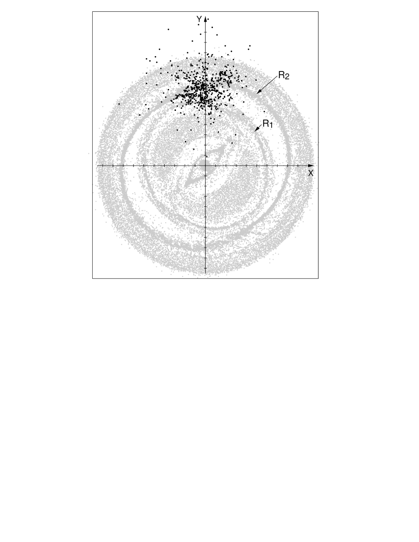
Fig. 1 : Distribution of young open clusters (black circles) from the catalog by Dias et al. (2002) and model particles (gray circles) in the Galactic plane. Only clusters with $\log\textrm{age}<8.00$ and located within 0.5 kpc ($|z|<0.5$ kpc) from the Galactic plane are considered. The positions of model particles (gas and OB particles) correspond to the position angle of the Sun with respect to the bar of $\theta_{\textrm{b}}=45^{\circ}$. The $X$-axis points in the direction of Galactic rotation and the $Y$-axis is directed away from the Galactic center. One tick interval along the $X$- and $Y$-axis corresponds to 1 kpc. The Sun is located at (0, 7.5 kpc). The arrows show the positions of the outer rings $R_{1}$ and $R_{2}$. Of the two rings, $R_{1}$ is located a bit closer to the Galactic center than the $R_{2}$.

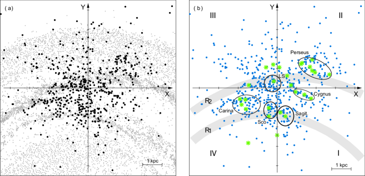
Fig. 2 : (a) Distribution of young ($\log\textrm{age}<8.00$) open clusters (black circles) from the catalog by Dias et al. (2002) and model particles (grey points) in the Galactic plane zoomed in to a larger scale. The Sun is at the origin. The positions of the model particles are drawn for $\theta_{\textrm{b}}=45^{\circ}$. The $X$-axis points in the direction of Galactic rotation and the $Y$-axis is directed away from the Galactic center. (b) The distribution of young open clusters (circles colored blue in electronic edition) and rich OB-associations (asterisks colored green in electronic edition) in the Galactic plane. Only OB-associations containing more than 30 members ($N_{t}>30$) in the catalogue by Blaha & Humphreys (1989) are shown. The locations of the outer rings $R_{1}$ and $R_{2}$ are indicated by gray arches. The positions of the Sagittarius, Scorpio, Carina, Cygnus, Local System (LS) and Perseus stellar-gas complexes are drawn by ellipses. The Sagittarius and Scorpio complexes are located in the vicinity of the ring $R_{1}$. The Perseus complex and Local System lie near the ring $R_{2}$. The Carina complex is situated in-between the two outer rings, where they seem to fuse together. As for the Cygnus complex, its connection with some global structure is unclear. Roman numerals show the numbers of quadrants.

1 Introduction

Open clusters are compact groups of stars born inside one giant molecular cloud during a short time interval. Young open clusters are gravitationally bound objects in distinction from OB-associations, which are loose groups of O and B-type stars. Such differences between young clusters and OB-associations are based on the comparison of their mass with the velocity dispersions inside them. The fact that all stars inside an open cluster have nearly the same age gives researchers the opportunity to fit the cluster main sequence and colour-colour diagrams to model grids derived from zero age main sequence (ZAMS) and a set of isochrones corresponding to different abundances. The result of fitting is the determination of many important physical characteristics of clusters, such as heliocentric distance, age, and metallicity (Kholopov, 1980; Mermilliod, 1981).

Young open clusters indicate the positions of giant molecular clouds but unlike gaseous objects, open clusters allow their distances to be determined quite precisely with an accuracy of $\sim 5\%$ as far as we ignore possible errors in the zero point of the adopted ZAMS (Dambis, 1999). So the concentration of young open clusters in some complexes suggests the presence of gas there and traces the positions of spiral arms and Galactic rings.

We suppose that the Galaxy contains a two-com-ponent outer ring $R_{1}R_{2}^{\prime}$ made up of two elliptical gaseous rings stretched perpendicularly to each other and located near the solar circle (Fig. 1). The sign of apostrophe means the pseudoring $R_{2}^{\prime}$ – incomplete ring made up of two tightly wound spiral arms. The idea that the Galaxy contains outer rings was first put forward by Kalnajs (1991).

Two main classes of outer rings and pseudorings have been identified: rings $R_{1}$ (pseudorings $R^{\prime}_{1}$) elongated perpendicular to the bar and rings $R_{2}$ (pseudorings $R^{\prime}_{2}$) elongated parallel to the bar. In addition, there is a combined morphological type $R_{1}R_{2}^{\prime}$ which exhibits elements of both classes (Buta, 1995; Buta & Combes, 1996; Buta & Crocker, 1991). Modelling shows that outer rings are usually located near the Outer Lindblad resonance (OLR) of the bar (Schwarz, 1981; Byrd et al., 1994; Rautiainen & Salo, 1999, 2000, and other papers).

Comeron et al. (2014) used the data from mid-infrared survey (Spitzer Survey of Stellar Structure in Galaxies, Sheth et al., 2010) to find that the frequency of outer rings is 16% for all spiral galaxies located inside 20 Mpc and over 40% for disk galaxies of early morphological types (galaxies with large bulges). The above authors have also found that the frequency of outer rings increases from $15\pm 2\%$ to $32\pm 7\%$ when going through the family sequence from SA to SAB, and decreases again to $20\pm 2\%$ for SB galaxies.

Note that the catalogue by Buta (1995) includes several tens of galaxies with rings $R_{1}R_{2}^{\prime}$. Here are some examples of galaxies with the $R_{1}R_{2}^{\prime}$ morphology that can be viewed as possible prototypes of the Milky Way: ESO 245-1, NGC 1079, NGC 1211, NGC 3081, NGC 5101, NGC 5701, NGC 6782, and NGC 7098. Their images can be found in de Vaucouleurs Atlas of Galaxies by Buta et al. (2007) at http://bama.ua.edu/ rbuta/devatlas/

There is extensive evidence for the existence of the bar in the Galaxy derived on the basis of infra-red observations (Blitz & Spergel, 1991; Benjamin et al., 2005; Cabrera-Lavers et al., 2007; González-Fernández et al., 2012; Churchwell et al., 2009) and gas kinematics in the central region (Binney et al., 1991; Englmaier & Gerhard, 1999; Weiner & Sellwood, 1999). The general consensus is that the major axis of the bar is oriented in the direction $\theta_{\textrm{b}}=15\textrm{--}45^{\circ}$ in such a way that the end of the bar closest to the Sun lies in quadrant I, where $\theta_{\textrm{b}}$ is the position angle between the line connecting the Sun and the Galactic center and the direction of the major axis of the bar. The semi-major axis of the Galactic bar is supposed to lie in the range $a=3.5\textrm{--}5.0$ kpc. Assuming that its end is located close to its corotation radius (CR), i.e. we are dealing with a so-called fast bar (Debattista & Sellwood, 2000), and that the rotation curve is flat, we can estimate the bar angular speed $\Omega_{b}$, which appears to be constrained to the interval $\Omega_{b}=40\textrm{--}65$ km s^-1 kpc^-1. This means that the OLR of the bar is located in the solar vicinity: $|R_{OLR}-R_{0}|<1.5$ kpc. Studies of the kinematics of old disk stars in the nearest solar neighbourhood, $r<250$ pc, reveal the bimodal structure of the distribution of ($u$, $v$) velocities, which is also interpreted to be a result of the solar location near the OLR of the bar (Dehnen, 2000; Fux, 2001, and other papers).

The explanation of the kinematics of young objects in the Perseus stellar-gas complex (see its location in Fig. 2b) is a serious test for different concepts of the Galactic spiral structure. The fact that the velocities of young stars in the Perseus stellar-gas complex are directed toward the Galactic center, if interpreted in terms of the density-wave concept (Lin et al., 1969), indicates that the trailing fragment of the Perseus arm must be located inside the corotation circle (CR) (Burton & Bania, 1974; Mel’nik et al., 2001; Mel’nik, 2003; Sitnik, 2003), and hence imposes an upper limit for its pattern speed $\Omega_{sp}<25$ km s^-1 kpc^-1, which is inconsistent with the pattern speed of the bar $\Omega_{b}=40\textrm{--}65$ km s^-1 kpc^-1 mentioned above.

The studies of Galactic spiral structure are usually based on the classical model developed by Georgelin & Georgelin (1976), which includes four spiral arms with a pitch angle of $\sim 12^{\circ}$ (see e.g.  the review by Vallée, 2013). The main achievement of this purely spiral model is that it can explain the distribution of HII regions in the Galactic disk (Russeil, 2003). This model became more physical after incorporation of the bar into it (Englmaier & Gerhard, 1999). However, the bar and spiral arms connected with it rotate with the angular speed $\Omega_{b}=50\textrm{--}60$ km s^-1 kpc^-1, and this model cannot explain the kinematics of young stars in the Perseus complex. Bissantz et al. (2003) developed the model of Englmaier & Gerhard (1999) by adding a pair of spiral arms rotating slower than the bar with $\Omega_{sp}=20$ km s^-1 kpc^-1. However, it remains unclear what mechanism can sustain this slower spiral pattern in the disk.

Liszt (1985) criticizes the use of kinematical distances for tracing the Galactic spiral structure. He shows that kinematical distances derived for HII regions, HI and CO clouds can be wrong due to kinematic-distance ambiguity and velocity perturbation from spiral arms. Moreover, Adler & Roberts (1992) show that bright spots in the diagrams (l, $V_{LSR}$) which are interpreted as ”clouds” can consist of a chain of clouds extending over several kpc along the line of sight.

Models of the Galaxy with the outer ring $R_{1}R_{2}^{\prime}$ reproduce well the radial and azimuthal components of the residual velocities (observed velocities minus the velocity due to the rotation curve and solar motion to the apex) of OB-associations in the Sagittarius (see its location in Fig. 2b) and Perseus complexes. The radial velocities of most OB-associations in the Perseus stellar-gas complex are directed toward the Galactic center and this indicates the presence of the ring $R_{2}$ in the Galaxy, while the radial velocities in the Sagittarius complex are directed away from the Galactic center suggesting the existence of the ring $R_{1}$. The nearly zero azimuthal component of the residual velocity of most OB-associations in the Sagittarius complex precisely constrains the solar position angle with respect to the bar major axis, $\theta_{\textrm{b}}=45\pm 5^{\circ}$. We considered models with analytical bars and N-body simulations (Mel’nik & Rautiainen, 2009; Rautiainen & Mel’nik, 2010).

The classical model of Galactic spiral structure can explain the existence of so-called tangential directions related to the maxima in the thermal radio continuum as well as HI and CO emission, which are associated with the tangents to the spiral arms (Englmaier & Gerhard, 1999; Vallée, 2008). Models of a two-component outer ring can also explain the existence of some of the tangential directions which, in this case, can be associated with the tangents to the outer and inner rings. Our model diagrams (l ,V${}_{\textrm{LSR}}$) reproduce the maxima in the direction of the Carina, Crux (Centaurus), Norma, and Sagittarius arms. Additionally, N-body model yields maxima in the directions of the Scutum and 3-kpc arms (Mel’nik & Rautiainen, 2011, 2013).

Pettitt at al. (2014) simulated the (l,V${}_{\textrm{LSR}}$) diagrams for models with analytical bar. Their gas disks form the two-component outer rings $R_{1}R_{2}$ 200–500 Myr after the start of the simulation. The above authors found observations to agree best with the model with the solar position angle of $\theta_{\textrm{b}}\approx 45^{\circ}$ and the bar pattern speed in the range of $\Omega_{b}=50\textrm{--}60$ km s^-1 kpc^-1.

Elliptic outer rings can be divided into the ascending and descending segments: in the ascending segments galactocentric distance $R$ decreases with increasing azimuthal angle $\theta$, which itself increases in the direction of galactic rotation, whereas in the descending segments distance $R$, on the contrary, increases with increasing angle $\theta$. Ascending and descending segments of the rings can be regarded as fragments of trailing and leading spiral arms, respectively. Note that if considered as fragments of the spiral arms, the ascending segments of the outer ring $R_{2}$ have the pitch angle of $\sim 6^{\circ}$ (Mel’nik & Rautiainen, 2011).

Schwarz (1981) associates two main types of outer rings with two main families of periodic orbits existing near the OLR of the bar (Contopoulos & Papayannopoulos, 1980). The main periodic orbits are followed by numerous chaotic orbits, and this guidance enables elliptical rings to hold a lot of gas in their vicinity. The rings $R_{1}$ are supported by $x_{1}(2)$-orbits (using the nomenclature of Contopoulos & Grosbol, 1989) lying inside the OLR and elongated perpendicular to the bar, while the rings $R_{2}$ are supported by $x_{1}(1)$-orbits located slightly outside the OLR and elongated along the bar. However, the role of chaotic and periodic orbits appears to be different inside and outside the CR of the bar: chaos is dominant outside corotation, while most orbits in the bar are ordered (Contopoulos & Patsis, 2006; Voglis et al., 2007). Not only periodic orbits induced by the bar and regular orbits related to them, but also manifolds connected to the unstable Lagrangian points near the ends of the bar, may contribute to the formation of outer rings and pseudorings (Romero-Gómez et al., 2007; Harsoula & Kalapotharakos, 2009; Athanassoula et al., 2010).

The study of classical Cepheids from the catalogue by Berdnikov et al. (2000) revealed the existence of ”the tuning-fork-like” structure in the distribution of Cepheids: at longitudes $l>180^{\circ}$ (quadrants III and IV) Cepheids concentrate strongly to the arm located near the Carina complex (the Carina arm), while at longitudes $l<180^{\circ}$ (quadrants I and II) there are two regions of high surface density located near the Perseus and Sagittarius complexes. The term ”the Carina arm” was used to designate the part of the Sagittarius-Carina arm (Fig. 11 in Georgelin & Georgelin, 1976) that starts near the Carina complex and continues to larger Galactocentric distances. In a morphological study the Carina arm cannot be distinguished from the ascending segment of the ring $R_{2}$. This morphology suggests that outer rings $R_{1}$ and $R_{2}$ come closest to each other somewhere near the Carina complex (see its location in Fig. 2b). We have also found some kinematical features in the distribution of Cepheids, which suggest the location of the Sun near the descending segment of the ring $R_{2}$ (Mel’nik et al., 2015).

In this paper we study the distribution and kinematics of young open clusters and OB-associations. Section 2 describes the models and catalogues used; Section 3 considers the morphological and kinematical features that suggest the existence of $R_{1}R_{2}^{\prime}$ ring in the Galaxy, and Section 4 presents the main conclusions.

2 Catalogues and Models

There are several large catalogues of open clusters. Dias et al. (2002) compiled a catalogue of the physical and kinematic parameters of open clusters using data reported by different authors. This catalogue, which is updated continuously, is available at http://www.astro.iag.usp.br/ocdb/ and presently lists 2167 clusters. Kharchenko et al. (2013) determined physical, structural and kinematic parameters of 3006 Galactic clusters. Mermilliod (1992) created WEBDA database of stars in open clusters (https://www.univie.ac.at/webda/), where positional, photometric and spectroscopic data for individual stars in cluster fields is stored. Mermilliod & Paunzen (2003) analysed these data and derived the astrophysical parameters (reddening, distance and age) of 573 open clusters.

In the last decade many embedded clusters (stellar groups recently born and still containing a lot of gas within their volumes) were detected from near- and mid-infrared surveys (see e. g.  the reviews by Glushkova, 2013; Morales et al., 2013). However, distances to most of these objects reman uncertain mainly because of the variable extinction law in the field of embedded clusters. The determination of their colour excesses requires detailed photometric and spectroscopic studies. For example, the estimates of the distance to the embedded cluster Westerlund 2 ranged from $r=2$ to 8 kpc, before a detailed study of this region has been carried out (Carraro et al., 2013). In this paper we consider only optically observed clusters.

For our study we have chosen the catalogue by Dias et al. (2002), which provides the most reliable estimates of distances, ages and other parameters. Its new version (3.4) contains 627 young clusters with the ages less than 100 Myr.

Paunzen & Netopil (2006) established a list of 72 ”standard” open clusters covering a wide range of ages, reddenings and distances selected on the basis of smallest errors from the available parameters in the literature. Their analysis is based on the averaged values from widely different methods and authors. The authors then compared the derived mean values with the parameters of open clusters published by Dias et al. (2002). They found that if one uses the parameters of the catalogue by Dias et al. (2002) then the expected errors are comparable with those derived by averaging the independent values from the literature. They concluded that ages, reddenings and distances in the catalog by Dias et al. (2002) are good for statistical research.

We adopted the proper motions of open clusters based on the Hipparcos catalogue (Hipparcos, 1997) from the paper by Baumgardt et al. (2000), and if they were absent there, from the catalogues by Glushkova et al. (1996, 1997), which are available at https://www.univie.ac.at/webda/elena.html. In the latter lists the proper motions were derived from the Four-Million Star Catalogue of positions and proper motions (4M-catalogue, Volchkov et al., 1992) and then reduced to the Hipparcos system. We chose these catalogues of proper motions because of the careful selection of star cluster members.

For kinematical study, we also use OB-associations from the list by Blaha & Humphreys (1989), which includes 91 objects. Their heliocentric distances $r_{\textrm{BH}}$ were reduced to the short distance scale $r=0.8\cdot r_{\textrm{BH}}$ (Sitnik & Mel’nik, 1996). The kinematical data were adopted from the catalogue by Mel’nik & Dambis (2009). The ages of OB-associations are supposed to be less than 30 Myr (Humphreys & McElroy, 1984; Bressan et al., 2012).

We use the simulation code developed by H. Salo (Salo, 1991; Salo & Laurikainen, 2000) to construct two different types of models (models with analytical bars and models based on N-body simulations), which reproduce the kinematics of OB-associations in the Perseus and Sagittarius complexes. Among many models with outer rings, we chose model 3 from the series of models with analytical bars (Mel’nik & Rautiainen, 2009) to compare with observations. This model has nearly flat rotation curve. The bar semi-axes are equal to $a=4.0$ kpc and $b=1.3$ kpc. The positions and velocities of $5\cdot 10^{4}$ model particles (gas+OB) are considered at time $T\approx 1$ Gyr from the start of the simulation. We scaled and turned this model with respect to the Sun to achieve the best agreement between the velocities of model particles and those of OB-associations in five stellar-gas complexes identified by Efremov & Sitnik (1988).

We adopt a solar Galactocentric distance of $R_{0}=7.5$ kpc (Rastorguev et al., 1994; Dambis et al., 1995; Glushkova et al., 1998; Nikiforov, 2004; Feast et al., 2008; Groenewegen et al., 2008; Reid at al., 2009b; Dambis et al., 2013; Francis & Anderson, 2014). As model 3 was adjusted for $R_{0}=7.1$ kpc, we rescaled all distances for model particles by a factor of $k=7.5/7.1$. Note that the particular choice of $R_{0}$ in the range 7 -9 kpc has practically no effect on the analysis of the morphology and kinematics of stars located within 3 kpc from the Sun.

3 Results

3.1 Space distribution of young open clusters

The distribution of young open clusters in the Galactic plane can reveal regions of intense star formation, which can be associated with spiral arms or Galactic rings. Figure 1 shows the distribution of young open clusters from the catalog by Dias et al. (2002) and model particles in the Galactic plane. Only clusters with ages less than 100 Myr and located within 0.5 kpc ($|z|<0.5$ kpc) from the Galactic plane are considered. We can see the model location of the outer rings $R_{1}$ and $R_{2}$ calculated for the solar position angle with respect to the bar major axis of $\theta_{\textrm{b}}=45^{\circ}$.

Figure 2a shows the distribution of young open clusters from the catalog by Dias et al. (2002) and model particles in a larger scale. To avoid cluttering with other objects, we made another plot (Fig. 2b), where we indicate the positions of rich OB-associations as well. The catalog by Blaha & Humphreys (1989) includes 27 rich OB-associations containing more than 30 members ($N_{t}>30$). Figure 2b also presents the positions of the Sagittarius, Scorpio, Carina, Cygnus, Local System and Perseus stellar-gas complexes from the list by Efremov & Sitnik (1988). We can see a tuning-fork-like structure in the distribution of young open clusters and OB-associations. At negative x-coordinates (on the left-hand side) most of the clusters concentrate to the only one arm (the Carina arm), while at positive x-coordinates (on the right-hand side) most of the clusters lie near the Perseus or the Sagittarius complexes. The Carina stellar-gas complex is located in-between the two outer rings, where they come closest to each other. The Sagittarius and Scorpio complexes lie near the ring $R_{1}$, while the Perseus complex and Local System, on the contrary, are situated near the ring $R_{2}$. In quadrant III, young objects within $r<1.5$ kpc concentrate to the Sun, while more distant objects distribute nearly randomly over a large area. As for the Cygnus complex, its connection with some global structure (outer ring or spiral arm) is unclear. However, the kinematics of young objects in the Cygnus complex is similar to that in the Perseus stellar-gas complex (Sitnik & Mel’nik, 1996, 1999), and we therefore tend to consider the Cygnus complex as a spur of the ring $R_{2}$, which can be rather lumpy.

Using the model distribution, we can quite accurately approximate the position of two outer rings by two ellipses oriented perpendicular to each other. The outer ring $R_{1}$ can be represented by the ellipse with the semi-axes $a_{1}=6.3$ and $b_{1}=5.8$ kpc, while the outer ring $R_{2}$ fits well the ellipse with $a_{2}=8.5$ and $b_{2}=7.6$ kpc. These values correspond to the solar Galactocentric distance $R_{0}=7.5$ kpc. The ring $R_{1}$ is stretched perpendicular to the bar and the ring $R_{2}$ is aligned with the bar, hence the position of the sample of open clusters with respect to the rings is determined by the position angle $\theta_{\textrm{b}}$ of the Sun with respect to the major axis of the bar. The outer rings do not touch each other because gas particles located on the orbits which cross near the OLR were scattered due to collisions during the formation of the outer rings. We now try to find the optimum angle $\theta_{\textrm{b}}$ providing the best agreement between the positions of the open clusters and the orientation of the outer rings.

Figure 3 shows the $\chi^{2}$ functions – the sums of normalized squared deviations (Press et al., 1987) of open clusters from the outer rings – calculated for different values of the angle $\theta_{\textrm{b}}$. Figure 3a shows the $\chi^{2}$ curve derived for the distribution of 564 young clusters located within $r<3.5$ kpc of the Sun. We can see a minimum at $\theta_{\textrm{min}}=35^{\circ}$ here. The random error of this estimate is of about $\pm 3^{\circ}$. Table 1 lists the parameters of the observed sample: the number $N$ of clusters, the standard deviation $\sigma$ of a cluster from the model position of the outer rings, and the angle $\theta_{\textrm{min}}$ corresponding to the minimum on the $\chi^{2}$ curve.

Figure 3b shows the $\chi^{2}$ functions computed for 10 random samples also containing 564 objects and distributed along the heliocentric distance $r$ in accordance with a power law $n(r)=r^{-1}$ that simulates the effect of selection (see section 3.2). An example of a such a random sample is shown in Figure 4a. The $\chi^{2}$ functions calculated for random samples demonstrate a plateau in the $0<\theta_{\textrm{b}}\leq 30^{\circ}$ range and a steep rise in the $30<\theta_{\textrm{b}}<90^{\circ}$ interval (Fig. 3b). A comparison of images shown in Figure 3a and Figure 3b indicates that the minimum at $\theta_{\textrm{min}}=35^{\circ}$ exists only on the curve obtained for the observed objects suggesting that it is not due to some specific best-fitting angles which are, in principle, possible in the cases involving only a small region of the Galactic plane.

Fig. 3 : The $\chi^{2}$ functions calculated for different values of the solar position angle $\theta_{\textrm{b}}$ with respect to the major axis of the bar. (a) The $\chi^{2}$ function derived for the distribution of 564 young clusters from catalog by Dias et al. (2002) located within $r<3.5$ kpc of the Sun. It has a minimum at $\theta_{\textrm{b}}=35\pm 3^{\circ}$. (b) The $\chi^{2}$ functions computed for 10 random samples containing 564 objects and distributed in the Galactic plane in accordance with the power law $n(r)\sim r^{-1}$ that simulates the effect of selection. We show one such sample in Fig. 4a. The $\chi^{2}$ curves calculated for random samples demonstrate a plateau at the $0<\theta_{\textrm{b}}\leq 30^{\circ}$ interval followed by a steep rise in the $30<\theta_{\textrm{b}}<90^{\circ}$ interval. The dissimilarity of the curves shown in ”a” and ”b” panels leads us to conclude that the minimum of the curve in panel ”a” is not due to some model effects.

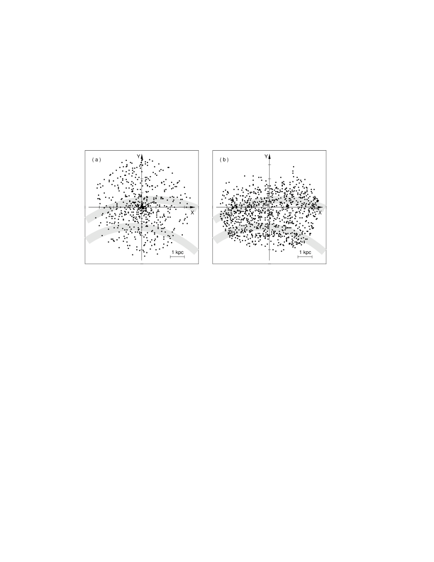
Fig. 4 : Examples of random samples generated to study selection effects. (a) Simulated objects are distributed in the Galactic plane in accordance with the power law $n(r)\sim r^{-1}$. The sample contains 564 objects. (b) Simulated objects are distributed near the outer rings at the Gaussian law with the standard deviation of $\sigma_{r}=0.8$ kpc. The ring $R_{2}$ is supposed to contain 64% of all objects. Only 20% of $N_{\textrm{mod}}=5000$ objects are shown. All simulated objects are located within 3.5 kpc from the Sun. The $X$-axis points in the direction of Galactic rotation and the $Y$-axis is directed away from the Galactic center. The Sun is at the origin.

Table 1 : Parameters of the sample

Sample	$N_{\textrm{obs}}$	$\sigma$	$\theta_{\textrm{min}}$
$0<r<3.5$ kpc	564	0.80 kpc	$35\pm 3^{\circ}$

We made some modifications to the observed sample to show how the overdensities in the Perseus and Carina complexes influence the shape of the $\chi^{2}$ function. Figure 5 shows the $\chi^{2}$ curves computed for the observed sample of open clusters after the mirror reflection of some regions with respect to the axis $Y$. All $\chi^{2}$ functions were calculated for the same number of objects $N_{\textrm{obs}}=564$. Sample designated as ”S1” was obtained from the observed distribution by changing ($l\to 360^{\circ}-l$) for objects located in quadrants II and III. In sample ”S1” the overdensity associated with the Perseus complex is located in quadrant III and the minimum of the corresponding $\chi^{2}$ curve becomes shallower in comparison with that obtained for the observed sample. This flattening of the $\chi^{2}$ curve is caused by the fact that the ring $R_{2}$ reaches larger $y$-coordinates in quadrant II than in quadrant III (Fig. 2). It is true for all values of $\theta_{\textrm{b}}$ from the expected interval 15–45^∘. Hence moving the Perseus complex into quadrant III increases deviations from the rings, and, consequently, increases the corresponding values of $\chi^{2}$.

Sample ”S2” (Fig. 5) is obtained by changing ($l\to 360^{\circ}-l$) for objects of quadrants IV and I, while objects of quadrants I and II are left at their original places. In sample ”S2” the overdensity associated with the Carina complex is located in quadrant I just between the rings $R_{1}$ and $R_{2}$. This transformation increases the deviations from the rings for objects of the Carina complex and causes the flattening the $\chi^{2}$ curve as well.

Sample ”S3” is a result of the ($l\to 360^{\circ}-l$) transformation of coordinates of all objects (Fig. 5). Here the overdensities associated with the Perseus and Carina complexes lie in quadrants III and I, respectively. We can see that the corresponding $\chi^{2}$ curve is practically flat in the interval $\theta_{\textrm{b}}=15\textrm{--}45^{\circ}$. The disappearance of the minimum here is due to the tuning-fork-like structure in the distribution of the observed objects. The mirror reflection creates the tuning-fork-like structure pointed in the opposite direction (one segment lies at positive $x$-coordinates and two segments are located at negative $x$-coordinates), which is inconsistent with the position of the outer rings obtained for $\theta_{\textrm{b}}=15\textrm{--}45^{\circ}$.

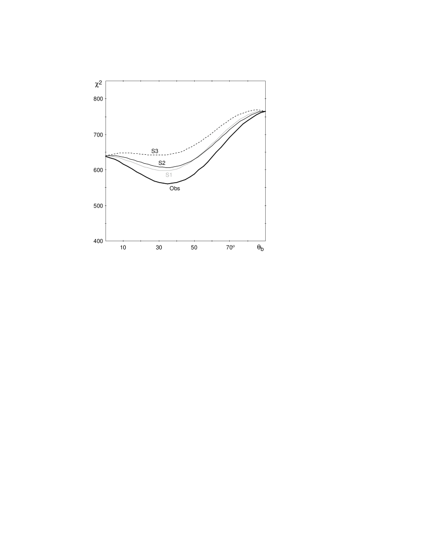
Fig. 5 : The $\chi^{2}$ functions computed for several samples of objects designated as ”Obs” (the thick solid line), ”S1” (the gray line),”S2” (the thin solid line), and ”S3” (the dashed line). The curve obtained for the observed sample of 564 young open clusters from the catalog by Dias et al. (2002) (”Obs”) has the deepest minimum. The modified sample ”S1” is obtained from the observed one by the mirror reflection of objects located in quadrants II and III with respect to the axis $Y$, which is identical with the ($l\to 360^{\circ}-l$) transformation. In sample ”S1” the overdensity associated with the Perseus stellar-gas complex is located in quadrant III. Sample ”S2” is obtained by changing ($l\to 360^{\circ}-l$) for objects located in quadrants IV and I, while objects of quadrants I and II are left at their original palaces. In sample ”S2” the overdensity associated with the Carina complex is located in quadrant I between the outer rigs $R_{1}$ and $R_{2}$. Sample ”S3” is made by applying the ($l\to 360^{\circ}-l$) transformation to all objects. Here the overdensities associated with the Perseus and Carina complexes are located in quadrants III and I, respectively. We can see that the $\chi^{2}$ curves calculated successively for the samples ”Obs”, ”S1”, ”S2”, and ”S3” have increasingly shallow minima.

Figure 6 shows the histogram of the deviations (minimal distances) $d$ of young open clusters from the model positions of the outer rings calculated for $\theta_{\textrm{b}}=35^{\circ}$. Here we can clearly see the concentration of observed clusters to the model positions of the outer rings. Deviations $d$ from the rings in the direction of the increasing $y$-coordinates are considered positive and those in the opposite direction are considered negative. The distribution of deviations can be approximated by the Gaussian law with a standard deviation of $\sigma=0.8$ kpc. The excess of positive deviations at $d>1.5$ kpc is due to clusters located in the direction of the anticenter. The fraction of clusters located in the vicinity of 1.5 kpc ($\sim 2\sigma$) from the rings appears to be 95%, which is in good agreement with the Gaussian law.

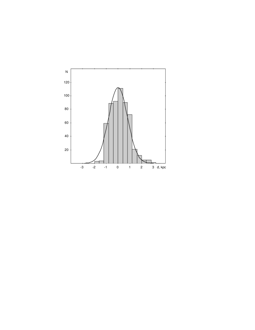
Fig. 6 : Distribution of the deviations (minimal distances) $d$ of young open clusters from the model positions of the outer rings calculated for $\theta_{\textrm{b}}=35^{\circ}$. It can be approximated by the Gaussian law with a standard deviation of $\sigma_{r}=0.8$ kpc (the solid line). Deviations from the rings in the direction of increasing $y$-coordinates are considered positive and those in the opposite direction are considered negative. The excess of positive deviations at $d>1.5$ kpc is due to clusters located in the direction of the anticenter. The fraction of clusters located within 1.5 kpc ($\sim 2\sigma$) of the rings appears to be 95%, as expected in the case of the Gaussian law.

We studied the effect of objects located in different regions on the location of the minimum of the $\chi^{2}$ curve. Removing the clusters located within the 0.5-kpc region ($r<0.5$ kpc) decreases $\theta_{\textrm{min}}$ from 35 to $30^{\circ}$. This shift appears due to the fact that the outer ring $R_{2}$ passes through the solar vicinity at angle $\theta_{\textrm{b}}=90^{\circ}$. So nearby clusters ”favour” greater $\theta_{\textrm{b}}$ values. However, there is also an opposite effect: excluding distant clusters located in the direction of the anticenter ($y>2.5$ kpc) from the observed sample increases $\theta_{\textrm{min}}$ from 35 to $40^{\circ}$. These clusters ($y>2.5$ kpc) are located far from both outer rings and therefore ”favour” the $\theta_{\textrm{b}}=0^{\circ}$ value in the case of which the ring $R_{2}$ crosses the $Y$-axis at maximum Galactocentric distance. We hence tend regard the uncertainty of $\pm 5^{\circ}$ as a random error of our method.

We made an attempt to simulate the influence of selection effects by assigning to every model object the probability $P$ of its detection. Generally, the detection of a cluster depends on a lot of things: the richness and angular size of a cluster, the number of resolved individual members and their visual brightness, the surface density of field stars, and the amount of extinction along the line of sight (Morales et al., 2013).

Let us suppose that the probability of detection of a cluster is determined mainly by the brightness of its stars. Then the probability of cluster detection is a function of its apparent distance modulus $DM$ which depends on the heliocentric distance to the cluster $r$ and the extinction $A_{V}$ toward it:

$$DM=5\lg r+10+A_{V},$$ (1)

where $r$ is in kpc.

The probability $P$ of detection of some objects is usually assumed to be equal to unity within some region of parameters and to be exponentially decreasing function beyond it. We can thus write the probability $P(DM)$ in the following way:

$$\begin{array}[]{cc}P(DM)=&\left\{\begin{array}[]{lcr}1&\textrm{if}&DM<DM_{0}\\ &&\\ e^{-(DM-DM_{0})/s_{0}}&\textrm{else,}&\\ \end{array}\right.\\ \end{array}$$ (2)

where the scale factor $s_{0}$ and zero point $DM_{0}$ are determined by fitting between the distributions of the distance moduli $DM$ of observed and model clusters.

To simulate the sample of clusters we adopted the value of the solar position angle $\theta_{\textrm{tru}}$ and scattered $N_{\textrm{mod}}=5000$ model objects with respect to the outer rings $R_{1}$ and $R_{2}$ in accordance with the Gaussian law with the standard deviation of $\sigma_{r}=0.8$ kpc within 3.5 kpc of the Sun, as it is shown in Figure 4b.

Note that among 564 young open clusters from the catalog by Dias et al. (2002) located within $r<3.5$ kpc, 408 objects ( 70%) appears to lie within 0.8 kpc from one of the two outer rings, of those 262 (64%) are located in the vicinity of the ring $R_{2}$. We therefore distributed simulated objects among two rings placing 64% of all objects in the ring $R_{2}$.

To calculate the distance modulus for a model object we must assign to it some value of the extinction $A_{V}$. That has been done in accordance with the extinction of observed young ($\log\textrm{age}<8.00$) clusters located in the nearby region and derived from their colour excess $A_{V}=3.1E_{B-V}$ (Cardelli et al., 1989). For each model objects situated at point (x, y) we selected observed young clusters from the catalog by Dias et al. (2002) located within the radius of $r_{e}=0.25$ kpc from the point (x, y), and calculated their average value of extinction $\overline{A_{V}}$. If there are less than $n_{e}<10$ observed clusters in the region of radius $r_{e}$ we successively increased the radius to $r_{e}=0.50$, 0.75, and 1.00 kpc. The radius $r_{e}=1.0$ kpc is the largest considered and the corresponding region always includes at least $n_{e}\geq 2$ observed clusters. Note that more than 93% of model objects have extinction estimates $\overline{A_{V}}$ averaged over $n_{e}>10$ observed young clusters.

The distance moduli $DM$ for model objects were calculated as follows:

$$DM=5\lg r+10+\overline{A_{V}}+\eta,$$ (3)

where $\eta$ is the error of the estimated distance modulus. We supposed that $\eta$ is distributed according to the Gaussian law with standard deviation $\sigma_{e}$, which is proportional to the average extinction $\overline{A_{V}}$ with some factor $k_{e}$:

$$\sigma_{e}=k_{e}\cdot\overline{A_{V}},$$ (4)

which is also determined, along with $s_{0}$ and $DM_{0}$, by fitting the distributions of distance moduli of model and observed objects.

Figure 7 shows the distributions of the distance moduli $DM$ of observed and model clusters. The model distribution is one of the best-fitting obtained with the parameters: $s_{0}=6.0^{m}$, $k_{e}=0.55$, and $DM_{0}=9.0^{m}$. The difference in calculating the model and observed distributions is that every model cluster is counted with the weight factor $P(DM)$, but not as unit entity as it was done for the observed distribution. We then normalize the model distribution so that it would contain the same number of clusters as the observed sample. Thus the normalized number of model clusters $N_{i}^{\textrm{mod}}$ in the bin $DM_{i-1}$– $DM_{i}$ is determined as follows:

$$N_{i}^{\textrm{mod}}=\sum_{k=1}^{k=j}P_{k}(DM)\cdot N_{\textrm{obs}}/N_{\textrm{mod}},$$ (5)

where $j$ is the number of model clusters in the distance-modulus bin considered, $P_{k}(DM)$ is the probability of their detection, $N_{\textrm{obs}}=564$ and $N_{\textrm{mod}}=5000$ are the numbers of observed and model clusters, respectively.

Table 2 : Study of selection effects

$\theta_{\textrm{tru}}$	$\theta_{\textrm{min}}$
$32.0^{\circ}$	$34.7\pm 1.2^{\circ}$
$33.0^{\circ}$	$35.5\pm 1.2^{\circ}$
$34.0^{\circ}$	$36.5\pm 1.2^{\circ}$
$35.0^{\circ}$	$37.5\pm 1.2^{\circ}$
$36.0^{\circ}$	$37.9\pm 1.1^{\circ}$
$37.0^{\circ}$	$38.8\pm 1.1^{\circ}$

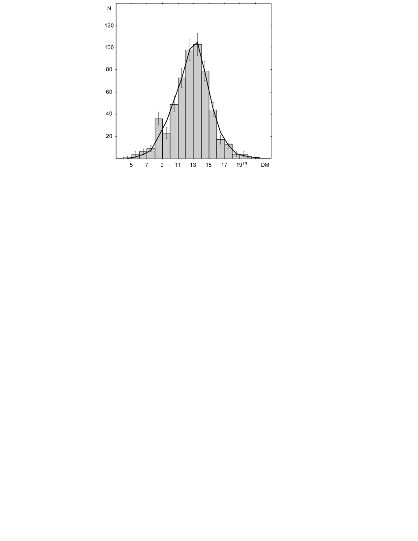
Fig. 7 : Distributions of the apparent distance moduli $DM$ for the observed and model clusters. The histogram shows the distribution of 564 observed clusters. The error bars show the uncertainty due to Poisson noise $\sqrt{N_{i}^{\textrm{obs}}}$. The solid line indicates one of the normalized distributions of model objects obtained for the best-fitting parameters: $s_{0}=6.0^{m}$, $k_{e}=0.55$, and $DM_{0}=9.0^{m}$.

We computed the $\chi^{2}$ statistic for fitting the distance modulus distributions of the model and observed clusters (Fig. 7) by the following formula:

$$\chi^{2}=\sum_{i=1}^{i=17}\frac{(N_{i}^{\textrm{mod}}-N_{i}^{\textrm{obs}})^{2}}{N_{i}^{\textrm{obs}}},$$ (6)

where the scatter in each column of the histogram (Fig. 7) is supposed to be due to the Poisson noise $\sim\sqrt{N_{i}^{\textrm{obs}}}$ and the number of bins is $i=17$.

Figure 8 shows the $\chi^{2}$ functions calculated from Eq. 6 plotted versus one of the parameters $s_{0}$, $k_{e}$, and $DM_{0}$ with all other fixed at their best-fitting values of $s_{0}=6.0$, $k_{e}=0.55$, and $DM_{0}=9.0^{m}$. The selection zero point $DM_{0}$ is determined very poorly, but its $\chi^{2}$ function demonstrates a kink near $\sim 9^{m}$, where the considerable growth follows the flat distribution. We can give only upper estimate of $DM_{0}$ equal to $\sim 9^{m}$, which in the case of zero extinction corresponds to $r_{0}=0.63$ kpc. Generally, extinction must not be large near the Sun and its presence must decrease the value of $r_{0}$ as well. Thus, the sample of young open clusters from the catalog by Dias et al. (2002) can be regarded as complete only within the radius $r<0.63$ kpc.

Fig. 8 : The behaviour of $\chi^{2}$ (Eq. 6) as a function of one of the parameters $s_{0}$, $k_{e}$, and $DM_{0}$ with all other parameters fixed at their best-fitting values of $s_{0}=6.0^{m}$, $k_{e}=0.55$, and $DM_{0}=9.0^{m}$. The error bars show the standard deviation in determination of the $\chi^{2}$ values and allows us to estimate the errors: $s_{0}=6.0\pm 1.2^{m}$, $k_{e}=0.55\pm 0.075$, and $DM_{0}=9.0^{+0.8m}_{-3.0}$. The parameter $DM_{0}$ is poorly determined, but its $\chi^{2}$ function shows a kink near $\sim 9^{m}$, where initially flat behavior turns into appreciable growth. Generally we can give only upper estimate for $DM_{0}$ equal to $\sim 9^{m}$.

Table 2 lists the values $\theta_{\textrm{tru}}$ of the angle $\theta_{\textrm{b}}$ used for simulating random samples and the calculated values $\theta_{\textrm{min}}$ derived from the location of the minimum of the $\chi^{2}$ curve. We determined the $\theta_{\textrm{min}}$ values for 200 simulated samples and then averaged them. A comparison of $\theta_{\textrm{tru}}$ and $\theta_{\textrm{min}}$ reveals a small bias $\Delta_{s}$, so that the calculated angles $\theta_{\textrm{min}}$ are always greater than their true values. For $\theta_{\textrm{min}}=35^{\circ}$ this bias equals $\Delta_{s}=-2.5^{\circ}$.

However, if we suppose that the probability of detection of model clusters is $P=1$ we obtain a systematical correction with the opposite sign, $\Delta_{s}=+5^{\circ}$, so that the calculated values are always smaller than the true ones. Generally, this shift is due to the objects located in the direction of the anticenter.

Note that the shift between the $\theta_{\textrm{tru}}$ and $\theta_{\textrm{min}}$ values decreases with decreasing the scatter $\sigma_{r}$ of model objects with respect to the outer rings.

We tend to regard the $\theta_{\textrm{b}}=35^{\circ}$ value as a good compromise to account for the combined effect of different factors. We summed the random $\pm 5^{\circ}$ and systematical $\pm 5^{\circ}$ errors because of their possible correlation to obtain an upper limit of $\sim 10^{\circ}$ for the combined error.

Note that our study of the sample of classical Cepheids yields $\theta_{\textrm{b}}=37\pm 13^{\circ}$ for the position angle of the Sun with respect to the bar’s major axis (Mel’nik et al., 2015). And the cause of this coincidence is that a tuning-fork-like structure is also present in the Cepheid distribution.

3.2 Surface density and extinction in different sectors

To study the distribution of clusters with respect to the Sun, we calculated their surface density in the Galactic plane. The variations in the surface density and extinction toward clusters provide some information about selection effects and the distribution of dust in the Galaxy. Here we verify the hypothesis that selection effects, if we consider their influence in $45^{\circ}$-width sectors of the Galactic plane, affect the sample of young clusters in nearly the same way irrespective of the direction, implying that the density maxima in the Carina and Perseus complexes can be attributed to real density enhancement rather than the lack of corresponding observations in other sectors.

To study selection effects, we subdivide the sample of young open clusters into 8 subsamples confined by $45^{\circ}$-width sectors: $l=0\textrm{--}45^{\circ}$, 45–90^∘, 90–135^∘, 135–180^∘, 180–225^∘, 225–270^∘, 270–315^∘, and 315–360^∘. For each sector we calculate the number of clusters in annuli of width $\Delta r=0.5$ kpc in the Galactic plane. The ratio of the number of clusters in 1/8-th of an annulus to its area gives us the average surface density of clusters in each sector per kpc². Table 3 lists the surface density values $n_{1}$, $n_{2}$,…, $n_{8}$ in different sectors derived for different distance intervals $r_{1}$ – $r_{2}$. It also gives the total surface density $n_{0}$ averaged over all sectors and the standard deviation $\sigma_{0}$ of the surface densities $n_{1}$, $n_{2}$,…, $n_{8}$ in sectors 1–8 from the average surface density $n_{0}$, which depends only on distance.

Figure 9a shows the variations of surface densities $n_{1}$, $n_{2}$,…, $n_{8}$, and $n_{0}$ along heliocentric distance $r$. The density maxima corresponding to the Carina and Perseus complexes are also indicated. The corresponding peaks of surface density are underlined in Table 3. The standard deviation $\sigma_{0}$ in the distance interval 0.5–3 kpc amounts, on average, to 40% of the total surface density $n_{0}(r)$. The errors $\sigma_{p}$ of the estimated surface density $n(r)$ in different sectors caused by the Poisson noise are, on average, twice smaller than the corresponding standard deviation $\sigma_{0}$ arising from the scatter of values obtained for different sectors. The average in the distance interval 1.5–2.5 kpc is $\overline{\sigma_{p}}=4$ cluster$\cdot$kpc^-2. The peaks in the Carina and Perseus complexes can be seen to deviate significantly from the total surface density $n_{0}(r)$ – the deviations amount to (1.9–2.1)$\sigma_{0}$ or $3\sigma_{p}$. We can hence conclude that these regions of enhanced density really exist at a significance level of $P\geq 2\sigma_{0}$. We cannot say the same of the Sagittarius complex (sector 1, $r=1\textrm{--}1.5$ kpc), where surface density exceeds the average value only by $0.7\sigma_{0}$ or $1.1\sigma_{p}$. However, this density peak extends beyond the corresponding sector and continues into the adjacent sector (sector 8, $r=1\textrm{--}1.5$ kpc) where density exceeds the average value by $1\sigma_{0}$ or $1.2\sigma_{p}$ (Table 3).

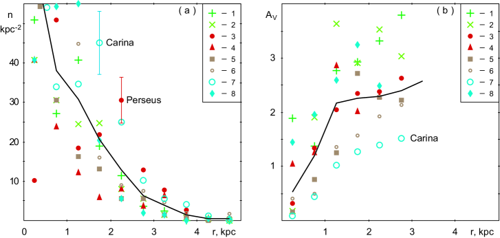
Fig. 9 : (a) Surface density $n$ in the Galactic plane calculated for young open clusters as a function of the heliocentric distance $r$ for 8 different sectors. Different symbols correspond to different sectors. In electronic edition four quadrants are represented by different colors. The errors of the computed surface density $n(r)$ in different sectors caused by the Poisson noise are, on average, twice smaller than the corresponding $\sigma_{0}$ values. The individual error bars are shown only for the Carina and Perseus complexes. The surface density $n_{0}$ averaged over all sectors is shown by a solid line. (b) The extinction $A_{V}$ along $r$ calculated for different sectors and $A^{0}_{V}$ averaged over all sectors (the solid line). The mean uncertainty of sector-averaged $A_{V}$ values is 0.4^m. The numbers 1–8 indicate the sectors: $l=0\textrm{--}45^{\circ}$ (1), 45–90^∘ (2), 90–135^∘ (3), 135–180^∘ (4), 180–225^∘ (5), 225–270^∘ (6), 270–315^∘ (7), and 315–360^∘ (8).

We assume that surface density of clusters decreases due to selection effects at a power law rate: $n(r)\sim r^{-\beta}$. We use seven surface density values in the interval 0–3.5 kpc to determine exponent $\beta$ and its error $\varepsilon_{\beta}$ for functions $n_{1}(r)$, $n_{2}(r)$,…, $n_{8}(r)$, and $n_{0}(r)$ (Table 3). The exponent $\beta$ derived for the total distribution $n_{0}(r)$ appears to be $\beta=1.03\pm 0.21$ and the corresponding exponents for different sectors, as a rule, coincide with this value within the errors. The only exception is the sector 180–225^∘ (5), where $\beta=1.62\pm 0.18$. The steep decline of surface density in this sector is possibly due to the physical lack of clusters in quadrant III.

Figure 9b demonstrates the variations of extinction $A_{V}$ toward open clusters along the distance $r$ in different sectors of the Galactic plane. We calculated extinction $A_{V}$ for each sector and each distance range based on the average colour excess of open clusters located there. Also shown is the average extinction $A^{0}_{V}(r)$ calculated for all sectors. The mean uncertainty of sector-averaged $A_{V}$ values is 0.4^m. Several interesting features are immediately apparent. First, extinction grows most rapidly in the sectors 0–45^∘ (1), 45–90^∘ (2) and 315–360^∘ (8). Second, the minimal values of extinction are observed in the direction of the Carina complex 270–315^∘ (7) and in the direction of the anticenter 225–270^∘ (6). Third, variations of extinction in the sector of the Perseus stellar-gas complex 90–135^∘ (3) are very close to those of average extinction $A^{0}_{V}$.

Note that we found similar features in variations of extinction for classical Cepheids (Mel’nik et al., 2015). Both groups of young objects, open clusters and Cepheids, show a sharp growth of extinction in the direction toward the Galactic center (see also Neckel & Klare, 1980; Marshall et al., 2006). This steep increase can be attributed to the presence of the Galactic outer ring $R_{1}$ at the heliocentric distance 1–2 kpc in this direction. The other feature – lower extinction in the direction of the Carina complex 270–315^∘ – can also be seen in the sample of classical Cepheids. Generally, low extinction in some direction means that the line of sight crosses interstellar medium with lower concentration of dust. Probably, there is a lack of dust in the space between the Sun and the Carina complex. The same is true for the anticenter direction. Moreover, lack of dust often correlates with lack of gas (Xu et al., 1997; Amôres & Lepine, 2005, and references therein).

Table 3 : Surface density in different sectors

$r_{1}$ – $r_{2}$	$n_{1}$	$n_{2}$	$n_{3}$	$n_{4}$	$n_{5}$	$n_{6}$	$n_{7}$	$n_{8}$	$n_{0}$	$\sigma_{0}$
	0–45∘	45–90∘	90–135∘	135–180∘	180–225∘	225–270∘	270–315∘	315–360∘	All
kpc			Perseus				Carina
0.0 – 0.5	50.9	40.7	10.2	40.7	173.2	122.2	71.3	40.7	68.8	53.3
0.5 – 1.0	27.2	30.6	50.9	23.8	30.6	54.3	34.0	54.3	38.2	12.8
1.0 – 1.5	40.7	24.4	18.3	12.2	16.3	44.8	34.6	55.0	30.8	15.3
1.5 – 2.0	18.9	24.7	21.8	5.8	13.1	16.0	45.1	20.4	20.7	11.5
2.0 – 2.5	11.3	7.9	30.6	7.9	5.7	9.1	24.9	5.7	12.9	9.5
2.5 – 3.0	3.7	5.6	13.0	3.7	5.6	7.4	10.2	1.9	6.4	3.7
3.0 – 3.5	2.4	1.6	7.8	6.3	1.6	4.7	5.5	1.6	3.9	2.5
$\beta$	1.08	1.05	0.97	0.89	1.62	1.28	0.79	1.34	1.03
$\varepsilon_{\beta}$	$\pm 0.34$	$\pm 0.35$	$\pm 0.36$	$\pm 0.15$	$\pm 0.18$	$\pm 0.19$	$\pm 0.27$	$\pm 0.50$	$\pm 0.21$
All values of surface density $n_{1}$, $n_{2}$,…, $n_{0}$, $\sigma_{0}$ are in the units of cluster$\cdot$kpc-2

3.3 Rotation curve

We use the sample of young ($\log\textrm{age}<8.00$) open clusters from the catalog by Dias et al. (2002) to determine the parameters of the rotation curve and compare them with those derived from the samples of OB-associations and classical Cepheids. We selected open clusters located within 3 kpc from the Sun and within 0.5 kpc ($|z|<0.5$ kpc) from the Galactic plane. In total, we have 187 young clusters with known proper motions, and 212 with known line-of-sight velocities. The line-of-sight velocities of clusters were taken from the catalogue by Dias et al. (2002, version 3.4). Of them $\sim 50\%$ were determined by Dias et al. (2014). We use only line-of-sight velocities and proper motions determined from the data for at least two cluster members ($n_{vr}\geq 2$, $n_{pm}\geq 2$). Of 187 cluster proper motions 53 were adopted from the list by Baumgardt et al. (2000) and the remaining 134 proper motions, from the list by Glushkova et al. (1996, 1997), which is available at http://www.sai.msu.su/groups/cluster/cl/pm/. The proper motions used in this study are derived or reduced to the Hipparcos system (Hipparcos, 1997).

We suppose that the motion of young objects in the disk obeys a circular rotation law. Then we can write the so-called Bottlinger equations for the line-of-sight velocities $V_{r}$ and proper motions along Galactic longitude $\mu_{l}$:

$$\begin{array}[]{l}V_{r}=R_{0}\cdot(\Omega-\Omega_{0})\cdot\sin l\cdot\cos b\\ \qquad-(u_{0}\cdot\cos l\cdot\cos b+v_{0}\cdot\sin l\cdot\cos b+w_{0}\cdot\sin b),\end{array}$$ (7)

$$\begin{array}[]{l}4.74\cdot\mu_{l}\cdot r=R_{0}\cdot(\Omega-\Omega_{0})\cdot\cos l-\Omega\cdot r\cdot\cos b\\ \qquad-(-u_{0}\cdot\sin l+v_{0}\cdot\cos l).\end{array}$$ (8)

The parameters $\Omega$ and $\Omega_{0}$ are the angular rotation velocities at the Galactocentric distance $R$ and at the distance of the Sun $R_{0}$, respectively. The velocity components $u_{0}$ and $v_{0}$ characterize the solar motion with respect to the centroid of objects considered in the direction toward the Galactic center and Galactic rotation, respectively. The velocity component $w_{0}$ is directed along the $z$-coordinate and we set it equal to $w_{0}=7.0$ km s^-1. The factor 4.74 converts the left-hand part of Eq. 8 (where proper motion and distance are in mas yr^-1 and kpc, respectively) into the units of km s^-1.

We expanded the angular rotation velocity $\Omega$ at Galactocentric distance $R$ into a power series in $(R-R_{0})$:

$$\Omega=\Omega_{0}+\Omega^{\prime}_{0}\cdot(R-R_{0})+0.5\cdot\Omega^{\prime\prime}_{0}\cdot(R-R_{0})^{2},$$ (9)

where $\Omega^{\prime}_{0}$ and $\Omega^{\prime\prime}_{0}$ are its first and second derivatives taken at the solar Galactocentric distance.

We simultaneously solve the equations for the line-of-sight velocities and proper motions. We also use weight factors $p_{vr}$ and $p_{vl}$ to balance the errors of line-of-sight and transversal velocity components:

$$p_{vr}=(\sigma_{0}^{2}+\varepsilon^{2}_{vr})^{-1/2},$$ (10)

$$p_{vl}=(\sigma_{0}^{2}+(4.74\cdot\varepsilon_{\mu l}\cdot r)^{2})^{-1/2},$$ (11)

where $\sigma_{0}$ is the so-called ”cosmic” velocity dispersion, which is approximately equal to the rms deviation of the velocities from the rotation curve (for more details see Dambis et al., 1995; Mel’nik et al., 1999; Mel’nik & Dambis, 2009). We adopted the errors of the line-of-sight velocities $\varepsilon_{vr}$ and proper motions $\varepsilon_{\mu l}$ from the corresponding catalogues.

We used an iterative cycle with 3$\sigma$ clipping to determine both the parameters of motion and the ”cosmic” velocity dispersion $\sigma_{0}$. At each iteration the line-of-sight velocities that deviate by more than $3\sigma_{0}$ from the computed rotation curve were eliminated. We also excluded proper motions which deviate by more than 6.0 mas yr^-1 ($3\cdot 2$ mas yr^-1, where 2 mas yr^-1 is the average error of proper motions considered) from the rotation curve. The rotation curve and solar motion parameters remain practically unchanged in subsequent iterations, but $\sigma_{0}$ decreases from 23 to 15 km s^-1. The final sample includes 156 and 209 equations for proper motions and line-of-sight velocities, respectively.

Table 4 lists the final values of the parameters of the rotation curve $\Omega_{0}$, $\Omega^{\prime}_{0}$, $\Omega^{\prime\prime}_{0}$ and solar motion $u_{0}$, $v_{0}$ and the final value of velocity dispersion $\sigma_{0}$ calculated for young open clusters. Also listed are the number of conditional equations $N$ and the value of Oort constant $A=-0.5R_{0}\Omega^{\prime}$. For comparison we also give the parameters derived for the sample of OB-associations (Mel’nik & Dambis, 2009) and those inferred for classical Cepheids (Mel’nik et al., 2015). We can see a good agreement between the parameters obtained for young open clusters and OB-associations (see also Fig. 10).

Note the large value of $\Omega_{0}=30.3\pm 1.2$ km s^-1 kpc^-1 obtained for young open clusters, which coincides with that calculated for OB-associations and maser sources, $\Omega_{0}=31\pm 1$ km s^-1 kpc^-1 (Reid at al., 2009a; Mel’nik & Dambis, 2009; Bobylev & Baikova, 2010). On the other hand, the angular velocity $\Omega_{0}$ at the solar Galactocentric distance estimated from the kinematics of Cepheids (Feast & Whitelock, 1997; Bobylev & Baikova, 2012) is systematically lower than the value derived from young open clusters and OB-associations. The parameters computed for young open clusters and Cepheids are consistent within the errors except for the second derivative $\Omega^{\prime\prime}_{0}$, which is equal to $1.65\pm 0.29$ and $1.07\pm 0.17$ km s^-2 kpc^-1, respectively (Table 4). Moreover, the rotation curve of Cepheids seems to be slightly descending, whereas that of OB-associations is nearly flat within the 3 kpc. The cause of this discrepancy is currently not clear.

The standard deviation of the velocities from the rotation curve equals $\sigma_{0}=15.2$, 7.16 and 10.84 km s^-1 for young open clusters, OB-associations and Cepheids, respectively (Table 4), which is consistent with other estimates (e.g.   Zabolotskikh et al., 2002). The larger value of $\sigma_{0}=15.2$ km s^-1 derived for clusters reflects the quality of the kinematical data rather than the physical scatter: all these objects are quite young, their ages do not exceed 200 Myr and they all must demonstrate the same physical scatter with respect to rotation curve to within 1–2 km s^-1. Possibly, the crowding in cluster fields prevents accurate measurements of line-of-light velocities and proper motions. Furthermore, the line-of-sight velocities of young open clusters are based on measured velocities of early-type stars, which usually have low accuracy because of the small number and large width of spectral lines involved.

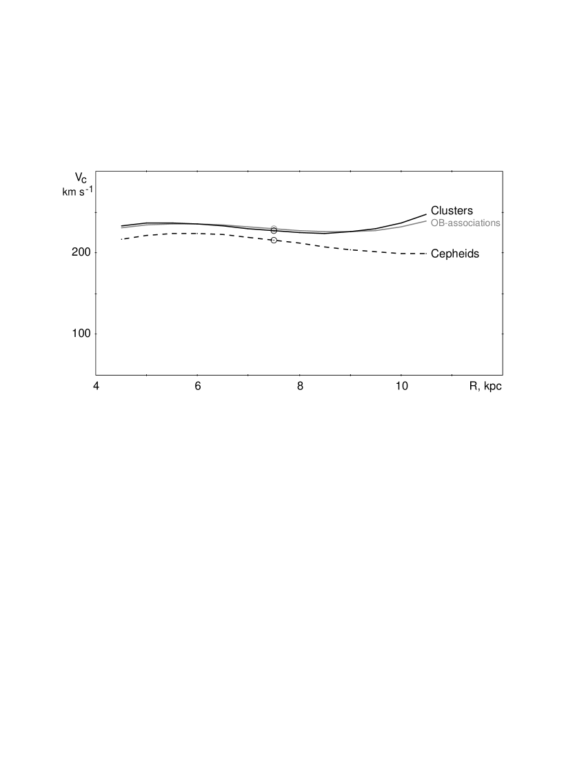
Fig. 10 : Galactic rotation curve derived from an analysis of line-of-sight velocities and proper motions of young open clusters (the black line), which practically coincides with that obtained for OB-associations (the gray line). The rotation curve computed for Cepheids lies systematically lower (the dashed line). The circle shows position of the Sun.

Table 4 : Parameters of the rotation curve and solar motion

Objects	$\Omega_{0}$	$\Omega^{\prime}_{0}$	$\Omega^{\prime\prime}_{0}$	$u_{0}$	$v_{0}$	A	$\sigma_{0}$	N
	km s-1	km s-1	km s-1	km s-1	km s-1	km s-1	km s-1
	kpc-1	kpc-2	kpc-3			kpc-1
Young open clusters	30.3	-4.73	1.65	9.8	11.1	17.7	15.20	365
$A<10^{8}$ yr	$\pm 1.2$	$\pm 0.24$	$\pm 0.29$	$\pm 1.3$	$\pm 1.5$	$\pm 0.9$
OB-associations	30.6	-4.73	1.43	7.7	11.6	17.7	7.16	132
	$\pm 0.9$	$\pm 0.18$	$\pm 0.21$	$\pm 1.0$	$\pm 1.3$	$\pm 0.7$
Classical Cepheids	28.8	-4.88	1.07	8.1	12.7	18.3	10.84	474
	$\pm 0.8$	$\pm 0.14$	$\pm 0.17$	$\pm 0.8$	$\pm 1.0$	$\pm 0.6$

3.4 Residual velocities of young open clusters and model particles

Residual velocities characterize non-circular motions in the Galactic disk. We calculated them as the differences between the observed heliocentric velocities and the computed velocities due to the circular rotation law and the adopted components of the solar motion defined by the parameters listed in Table 4 (first line). For model particles the residual velocities are determined with respect to the model rotation curve. We consider the residual velocities in the radial $V_{R}$ and azimuthal $V_{T}$ directions. Positive radial residual velocities $V_{R}$ are directed away from the Galactic center, while positive azimuthal residual velocities $V_{T}$ are in the sense of Galactic rotation.

The velocity field of gas clouds moving along the outer elliptic galactic rings is characterized by alternation of the negative and positive radial residual velocities $V_{R}$ directed toward and away from the galactic center, respectively (Mel’nik & Rautiainen, 2009). In the ascending segments of the rings (trailing spiral fragments) gas clouds have positive velocities $V_{R}$ directed away from the galactic center, while in the descending segments (leading spiral fragments), on the contrary, $V_{R}$ is directed toward the center. This becomes clear when we remember that outer rings lie outside the CR of the bar. Hence, in the reference frame co-rotating with the bar gas clouds rotate along the outer rings in the sense opposite that of galactic rotation, i.e. move in the sense of decreasing azimuthal angle $\theta$. In the descending segments, as defined, galactocentric distance $R$ increases with increasing azimuthal angle $\theta$ (leading spiral arm fragments), but if objects rotate in the sense of decreasing angle $\theta$ the distance $R$ must decrease. So in the descending segments of the outer rings objects must approach the galactic center. In the 3 kpc solar neighborhood there is only one descending segment of the outer rings – that of the ring $R_{2}$. Hence within 3 kpc of the Sun, objects with negative velocities $V_{R}$ must outline the location of the ring $R_{2}$.

Figure 11a shows the distribution of young open clusters ($\log\textrm{age}<8.00$) and OB-associations with negative radial residual velocities ($V_{R}<0$) in the Galactic plane. The sample includes 90 objects (57 clusters and 33 OB-associations) located within 3 kpc from the Sun. We consider only OB-associations with the line-of-sight velocity and proper motion based on data for at least two cluster members ($n_{vr}\geq 2$, $n_{pm}\geq 2$), and the same is true for open clusters. Within $r<3.0$ kpc from the Sun, the elliptic ring $R_{2}$ can be represented as a fragment of the leading spiral arm. We solve 90 equations by $\chi^{2}$-minimization (Press et al., 1987) to find the parameters of the spiral law. The pitch angle of the spiral-arm derived from clusters and OB-associations appears to be $i=20\pm 5^{\circ}$. The positive value of the pitch angle $i$ indicates that Galactocentric distance $R$ increases with increasing azimuthal angle $\theta$ what corresponds to the leading spiral arm fragment and suggests the solar position near the descending segment of the outer ring. Both types of objects, young clusters and OB-associations, give the same result: $i=19.3\pm 6.7^{\circ}$ and $i=20.3\pm 6.4^{\circ}$, respectively. Obviously, these objects demonstrate similar behavior.

Note that the pitch angle $i=20\pm 5^{\circ}$ obtained for clusters and OB-associations differs strongly from the value derived for model particles $i=6.6\pm 0.6^{\circ}$. The cause of this discrepancy is that objects of the Perseus and Carina complexes deviate from the smooth contour of the outer ring $R_{2}$. If we exclude the most distant parts of these regions, for example, by reducing the neighborhood considered from 3 to 2 kpc from the Sun, the pitch angle estimate decreases from $i=20\pm 5^{\circ}$ to $i=11.4\pm 5.3^{\circ}$. The latter value was derived for 60 objects (39 clusters and 21 OB-associations) located within $r<2$ kpc of the Sun. The values of $i=11.4\pm 5.3^{\circ}$ and $i=6.6\pm 0.6^{\circ}$ obtained for observed objects and model particles are consistent within the errors. The value of $i=11.4\pm 5.3^{\circ}$ is positive at the significance level $P>2\sigma$, which means that the spiral fragment to which young open clusters and OB-associations concentrate is leading.

In this context the question of the ragged structure of the ring $R_{2}$ comes up. Though the deviations from the smooth contour of the ring $R_{2}$ can result from errors in the parameters of distant objects, there is another aspect of the problem. A two-component outer ring $R_{1}R_{2}$ usually includes not just a pure $R_{2}$ ring but a pseudoring $R_{2}^{\prime}$ (broken ring) (Buta, 1995). Such deviations from pure ring morphology are also observed in numerical simulations (e.g. Rautiainen & Salo, 2000, Figure 3) with the break usually located on the descending segment of the ring. Hence the fact that the Perseus and Carina complexes deviate from the smooth elliptic segment in different directions – away from the Galactic center in the Perseus stellar-gas complex and toward the center in the Carina complex – may indicate the pseudoring morphology. This question requires further study.

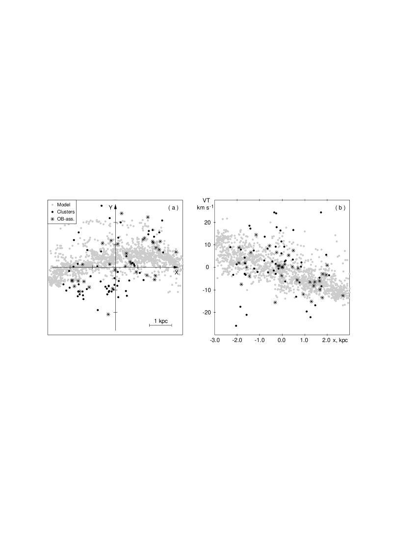
Fig. 11 : Comparison of the distribution of young open clusters ($\log\textrm{age}<8.00$) (the circles colored blue in electronic edition) and OB-associations (the asterisks colored green in electronic edition) with that of model particles (gray circles). We selected only objects with radial residual velocities directed toward the Galactic center ($V_{R}<0$). The positions of model particles (gas and OB particles) are calculated for the solar position angle $\theta_{\textrm{b}}=45^{\circ}$. (a) Distribution of observed objects and model particles in the Galactic plane. The selected clusters and OB-associations must outline the descending segment of the outer ring $R_{2}$, i. e. concentrate to a fragment of a leading spiral. The $X$-axis is directed in the sense of the Galactic rotation and the $Y$-axis, away from the Galactic center. The Sun is at the origin. (b) Dependence of azimuthal residual velocity $V_{T}$ on coordinate $x$ for objects with $V_{R}<0$. All objects demonstrate the decrease in $V_{T}$ with increasing $x$.

The residual azimuthal velocity $V_{T}$ also oscillates along the elliptic ring. These oscillations are shifted by $\pi/4$ in phase with respect to those of the radial velocity $V_{R}$ and are associated with ordered epicyclic motion of gas clouds and young stars near the OLR of the bar (Mel’nik & Rautiainen, 2009).

Figure 11b shows the dependence of azimuthal residual velocity $V_{T}$ on coordinate $x$ for young open clusters, OB-associations and model particles with negative radial residual velocities ($V_{R}<0$). These objects are supposed to belong to the descending segment of the outer ring $R_{2}$ and must show the decrease of $V_{T}$ with increasing $x$. The regression coefficient calculated for young clusters and OB-associations located within 3 kpc of the Sun is $k=-1.85\pm 0.90$ and differs significantly from the value calculated for model particles $k=-3.45\pm 0.07$. However, if we leave only OB-associations we would get $k=-3.03\pm 0.85$, which is negative at significance level of $P>3\sigma$ and agrees well with the model value.

4 Discussion and conclusions

We study the distribution and kinematics of young open clusters from the catalogue by Dias et al. (2002) in terms of the model of the Galactic ring $R_{1}R_{2}^{\prime}$ (Mel’nik & Rautiainen, 2009). The best agreement between the distribution of observed clusters and model particles is achieved for the solar position angle of $\theta_{\textrm{b}}=35\pm 10^{\circ}$ with respect to the bar major axis. It is due to of ”the tuning-fork-like” structure in the distribution of clusters: at negative x-coordinates most of the clusters concentrate to the only one arm (the Carina arm), while at positive x-coordinates most of the clusters lie near the Perseus or the Sagittarius complexes (Fig. 2).

We studied the influence of objects located in different regions on the position of the minimum of the $\chi^{2}$ curve. Excluding the clusters lying within the 0.5-kpc region ($r<0.5$ kpc) from the observed sample decreases the value of $\theta_{\textrm{min}}$ from 35 to $30^{\circ}$, while the exclusion of distant clusters located in the direction of the anticenter ($y>2.5$ kpc) increases $\theta_{\textrm{min}}$ from 35 to $40^{\circ}$.

We performed mirror reflection of the distribution of observed clusters with respect to the $Y$-axis, which is identical to the ($l\to 360^{\circ}-l$) transformation. The reflection obliterates the minimum of the $\chi^{2}$ curve. After the reflection clusters form a tuning-fork-like structure pointed in the opposite direction (one segment at the positive $x$-coordinates and two segments at the negative $x$-coordinates), which is inconsistent with the position of the outer rings calculated for $\theta_{\textrm{b}}=15\textrm{--}45^{\circ}$.

We simulated the influence of selection effects by assigning to every model object the probability $P$ of its detection depending on its apparent distance modulus $DM$. The probability $P$ is assumed to be equal to unity for $DM<DM_{0}$ and decrease exponentially with $DM$ at $DM\geq DM_{0}$ (Eq. 2). We determined the parameters of the dependence $P(DM)$ by fitting the distributions of distance moduli $DM$ of the observed and model clusters (Figs. 7, 8). We computed the extinction $A_{V}$ for model objects in accordance with the extinction of observed clusters located in the nearby region. We scattered the model clusters in the vicinity of the model positions of the outer rings and computed the $\chi^{2}$ function for 200 model samples. A comparison of the $\theta_{\textrm{tru}}$ and $\theta_{\textrm{min}}$ values reveals a small bias $\Delta_{s}=-2.5^{\circ}$ which does not exceed the random errors of $\pm 5^{\circ}$ (Table 2).

We consider the value of $\theta_{\textrm{b}}=35^{\circ}$ as a good compromise reflecting the combined influence of different effects. The upper limit of the combined error including random and systematic errors is $\pm 10^{\circ}$.

An analysis of the surface density $n$ of young clusters in different sectors of the Galactic plane suggests a weak dependence of selection effects on the direction. We found that extinction $A_{V}$ toward open clusters grows most rapidly in the direction of the Galactic center ($l=315\textrm{--}360^{\circ}$ and 0–45^∘) and in the sector 45–90^∘, while it is minimal in the direction of the the Carina complex 270–315^∘ and the anticenter 225–270^∘. Note that we found similar features in the variations of extinction for classical Cepheids (Mel’nik et al., 2015). Possibly, the sharp growth of extinction can be attributed to the presence of the Galactic outer ring $R_{1}$ at the heliocentric distance 1–2 kpc in the direction to the Galactic center.

The parameters of the rotation curve derived from the sample of young open clusters agree well with those obtained for OB-associations (Mel’nik & Dambis, 2009, Table 4). The rotation curve is nearly flat in the 3 kpc solar neighborhood with the large value of the Galactic angular velocity at the solar radius $\Omega_{0}=30.3\pm 1.2$ km s^-1 kpc^-1.

We study the distribution of young open clusters and OB-associations with negative radial residual velocities $V_{R}$, which within 3 kpc of the Sun must outline the descending segment of the ring $R_{2}$. Clusters and OB-association demonstrate similar distribution in the Galactic plane: objects of both types concentrate to the fragment of the leading spiral arm (see also Mel’nik, 2005). Within 2 kpc from the Sun, the pitch angles of the spiral fragment derived for model particles $i=6.0\pm 0.5^{\circ}$ and observed objects $i=11.4\pm 5.3^{\circ}$ are consistent within the errors.

We also found the azimuthal velocity $V_{T}$ to decrease with increasing coordinate $x$ for objects with negative radial residual velocities ($V_{R}<0$). The regression coefficient calculated for 33 OB-associations located within 3 kpc of the Sun, $k=-3.03\pm 0.85$, agrees well with the value $k=-3.45\pm 0.07$ calculated for model particles.

The morphological and kinematical features discussed have also been found for the sample of classical Cepheids (Mel’nik et al., 2015). Thus, all types of objects – young open clusters, OB-associations and classical Cepheids – suggest the presence of the outer ring $R_{1}R_{2}^{\prime}$ in the Galaxy.

References

- Adler & Roberts (1992) Adler, D. S., Roberts, W. W.: 1992, Astrophys. J., 384, 95
- Amôres & Lepine (2005) Amôres, E. B., Lepine, J. R. D.: 2005, Astron. J., 130, 659
- Athanassoula et al. (2010) Athanassoula, E., Romero-Gómez, M., Bosma, A., Masdemont, J. J.: 2010, Mon. Not. R. Astron. Soc., 407, 1433
- Baumgardt et al. (2000) Baumgardt, H., Dettbarn, C., & Wielen, R.: 2000, Astrophys. J. Suppl. Ser., 146, 251
- Benjamin et al. (2005) Benjamin, R. A. et al.: 2005, Astrophys. J., 630, L149
- Berdnikov et al. (2000) Berdnikov, L. N., Dambis, A. K., Vozyakova, O. V.: 2000, Astrophys. J. Suppl. Ser., 143, 211
- Binney et al. (1991) Binney, J., Gerhard, O., Stark, A. A., Bally, J., Uchida, K. I.: 1991, Mon. Not. R. Astron. Soc., 252, 210
- Bissantz et al. (2003) Bissantz, N., Englmaier, P., Gerhard, O.: 2003 Mon. Not. R. Astron. Soc., 340, 949
- Blaha & Humphreys (1989) Blaha, C., Humphreys, R. M.: 1989, Astron. J., 98, 1598
- Blitz & Spergel (1991) Blitz, L., Spergel, D. N.: 1991, Astrophys. J., 379, 631
- Bobylev & Baikova (2010) Bobylev, V. V., Baikova, A. T.: 2010, Mon. Not. R. Astron. Soc., 408, 1788
- Bobylev & Baikova (2012) Bobylev, V. V., Baikova, A. T.: 2012, Astron. Lett., 38, 638
- Bressan et al. (2012) Bressan, A., Marigo, P., Girardi, L., Salasnich, B., Dal Cero, C., Rubele, S., Nanni, A.: 2012, Mon. Not. R. Astron. Soc., 427, 127
- Burton & Bania (1974) Burton, W. B., Bania, T. M.: 1974, Astron. Astrophys., 33, 425
- Buta (1995) Buta, R.: 1995, Astrophys. J. Suppl. Ser., 96, 39
- Buta & Combes (1996) Buta, R., Combes, F.: 1996, Fundam. Cosmic Phys., 17, 95
- Buta & Crocker (1991) Buta, R., Crocker, D. A.: 1991, Astron. J., 102, 1715
- Buta et al. (2007) Buta, R., Corwin, H. G., Odewahn, S. C. 2007, The de Vaucouleurs Atlas of Galaxies, Cambridge Univ. Press., Cambridge
- Byrd et al. (1994) Byrd, G., Rautiainen, P., Salo, H., Buta, R., Crocker, D. A.: 1994, Astron. J., 108, 476
- Cabrera-Lavers et al. (2007) Cabrera-Lavers, A., Hammersley, P. L., González-Fernández, C., López-Corredoira, M., Garzón, F., Mahoney, T. J.: 2007, Astron. Astrophys., 465, 825
- Cardelli et al. (1989) Cardelli, J. A., Clayton, G. C., Mathis, J. S.: 1989, Astrophys. J., 345, 245
- Carraro et al. (2013) Carraro, G., Turner, D., Majaess, D., Baume, G.: 2013, Astron. Astrophys., 555, 50
- Churchwell et al. (2009) Churchwell, E. et al.: 2009, Publ. Astron. Soc. Pac., 121, 213
- Comeron et al. (2014) Comerón, S. et al.: 2014, Astron. Astrophys., 562, 121
- Contopoulos & Grosbol (1989) Contopoulos, G., Grosbol, P.: 1989, Astron. Astrophys. Rev., 1, 261
- Contopoulos & Papayannopoulos (1980) Contopoulos, G., Papayannopoulos, Th.: 1980, Astron. Astrophys., 92, 33
- Contopoulos & Patsis (2006) Contopoulos, G., Patsis, P. A.: 2010, Mon. Not. R. Astron. Soc., 369, 1039
- Dambis et al. (1995) Dambis, A. K., Mel’nik, A. M., Rastorguev, A. S.: 1995, Astron. Lett., 21, 291
- Dambis (1999) Dambis, A. K.: 1999, Astron. Lett., 25, 7
- Dambis et al. (2013) Dambis, A. K., Berdnikov, L. N., Kniazev, A. Y., Kravtsov, V. V., Rastorguev, A. S., Sefako, R., Vozyakova, O. V.: 2013, Mon. Not. R. Astron. Soc., 435, 3206
- Debattista & Sellwood (2000) Debattista, V. P., Sellwood, J. A.: 2000, Astrophys. J., 543, 704
- Dehnen (2000) Dehnen, W.: 2000, Astron. J., 119, 800
- Dias et al. (2002) Dias, W. S., Alessi, B. S., Moitinho, A., Lepine, J. R. D.: 2002, Astron. Astrophys., 389, 871
- Dias et al. (2014) Dias, W. S., Monteiro, H., Caetano, T. C., Lepine, J. R. D., Assafin, M., Oliveira, A. F.: 2014, Astron. Astrophys., 564, 79
- Efremov & Sitnik (1988) Efremov, Y. N., Sitnik, T. G.: 1988, Soviet Astron. Lett., 14, 347
- Englmaier & Gerhard (1999) Englmaier, P., Gerhard, O.: 1999, Mon. Not. R. Astron. Soc., 304, 512
- Hipparcos (1997) ESA 1997, The Hipparcos and Tycho Catalogues, ESA SP-1200, Noordwijk
- Feast & Whitelock (1997) Feast, M. W., Whitelock, P. A.: 1997, Mon. Not. R. Astron. Soc., 291, 683
- Feast et al. (2008) Feast, M. W., Laney, C. D., Kinman, T. D., van Leeuwen, F., Whitelock, P. A.: 2008, Mon. Not. R. Astron. Soc., 386, 2115
- Francis & Anderson (2014) Francis, Ch., Anderson, E.: 2014, Mon. Not. R. Astron. Soc., 441, 1105
- Fux (2001) Fux, R.: 2001, Astron. Astrophys., 373, 511
- Georgelin & Georgelin (1976) Georgelin, Y. M., Georgelin, Y. P.: 1976, Astron. Astrophys., 49, 57
- Glushkova (2013) Glushkova, E. V.: 2013, AN, 334, 843
- Glushkova et al. (1996) Glushkova, E. V., Zabolotskikh, M. V., Rastorguev, A. S., Uglova, I. M., Fedorova, A. A., Volchkov, A. A.: 1996, Astron. Lett., 22, 764
- Glushkova et al. (1997) Glushkova, E. V., Zabolotskikh, M. V., Rastorguev, A. S., Uglova, I. M., Fedorova, A. A.: 1997, Astron. Lett., 23, 71
- Glushkova et al. (1998) Glushkova, E. V., Dambis, A. K., Mel’nik, A. M., Rastorguev, A. S.: 1998 Astron. Astrophys.329, 514
- González-Fernández et al. (2012) González-Fernández, C., López-Corredoira, M., Amôres, E. B., Minniti, D., Lucas, P., Toledo, I.: 2012, Astron. Astrophys., 546, 107
- Groenewegen et al. (2008) Groenewegen, M. A. T., Udalski, A., Bono, G.: 2008, Astron. Astrophys., 481, 441
- Harsoula & Kalapotharakos (2009) Harsoula, M., Kalapotharakos, C.: 2009, Mon. Not. R. Astron. Soc., 394, 1605
- Humphreys & McElroy (1984) Humphreys, R. M, McElroy, B.: 1984, Astrophys. J., 284, 565
- Kalnajs (1991) Kalnajs, A. J. 1991, in Sundelius, B., ed., Dynamics of Disk Galaxies. Göteborgs Univ., Göthenburg, p. 323
- Kharchenko et al. (2013) Kharchenko, N. V., Piskunov, A. E., Röser, S., Schilbach, E., Scholz, R.-D.: 2013, Astron. Astrophys., 558, 53
- Kholopov (1980) Kholopov, P. N.: 1980, Soviet Astron., 24, 7
- Lin et al. (1969) Lin, C. C., Yuan, C., Shu, F. H.: 1969, Astrophys. J., 155, 721
- Liszt (1985) Liszt, H. S. 1985, in H. van Woerden et al., eds, Proc. IAU Symp. 106, The Milky Way Galaxy. Dordrecht, D. Reidel Publishing Co., p. 283
- Marshall et al. (2006) Marshall, D. J., Robin, A. C., Reyle, C., Schultheis, M., Picaud, S.: 2006, Astron. Astrophys., 453, 635
- Mel’nik (2003) Mel’nik, A. M.: 2003, Astron. Lett., 29, 304
- Mel’nik (2005) Mel’nik, A. M.: 2005, Astron. Lett., 31, 80
- Mel’nik & Dambis (2009) Mel’nik, A. M., Dambis, A. K.: 2009, Mon. Not. R. Astron. Soc., 400, 518
- Mel’nik & Rautiainen (2009) Mel’nik, A. M., Rautiainen, P.: 2009, Astron. Lett., 35, 609
- Mel’nik & Rautiainen (2011) Mel’nik, A. M., Rautiainen, P.: 2011, Mon. Not. R. Astron. Soc., 418, 2508
- Mel’nik & Rautiainen (2013) Mel’nik, A. M., Rautiainen, P.: 2013, AN, 334, 777
- Mel’nik et al. (1999) Mel’nik, A. M., Dambis, A. K., Rastorguev, A. S.: 1999, Astron. Lett., 25, 518
- Mel’nik et al. (2001) Mel’nik, A. M., Dambis, A. K., Rastorguev, A. S.: 2001, Astron. Lett., 27, 521
- Mel’nik et al. (2015) Mel’nik, A. M., Rautiainen, P., Berdnikov, L. N., Dambis, A. K., Rastorguev, A. S.: 2015, AN, 336, 70
- Mermilliod (1981) Mermilliod, J.-C.: 1981, Astron. Astrophys., 97, 235
- Mermilliod (1992) Mermilliod, J.-C.: 1992, Bull. Inform. CDS, 40, 115
- Mermilliod & Paunzen (2003) Mermilliod, J.-C., Paunzen, E.: 2003, Astron. Astrophys., 410, 511
- Morales et al. (2013) Morales, E. F. E., Wyrowski, F., Schuller, F., Menten, K.,: 2013, Astron. Astrophys., 560, 76
- Neckel & Klare (1980) Neckel, Th., Klare, G.: 1980, Astrophys. J. Suppl. Ser., 42, 251
- Nikiforov (2004) Nikiforov, I. I. 2004, ASP Conf. Ser. Vol. 316, Astron. Soc. Pac., San Francisco, p. 199
- Paunzen & Netopil (2006) Paunzen, E., Netopil, M.: 2006, Mon. Not. R. Astron. Soc., 371, 1641
- Pettitt at al. (2014) Pettitt, A. R., Dobbs, C. L., Acreman, D. M., Price, D. J.: 2014, Mon. Not. R. Astron. Soc., 444, 919
- Press et al. (1987) Press, W. H., Flannery, B. P., Teukolsky, S. A., Wetterling, W. T., Kriz, S. 1987, Numerical Recipes: The Art of Scientific Computing, Cambridge Univ. Press, Cambridge
- Rastorguev et al. (1994) Rastorguev, A. S., Pavlovskaya, E. D., Durlevich, O. V., Filippova, A. A.: 1994, Astron. Lett., 20, 591
- Rautiainen & Mel’nik (2010) Rautiainen, P., Mel’nik, A. M.: 2010, Astron. Astrophys., 519, 70
- Rautiainen & Salo (1999) Rautiainen, P., Salo, H.: 1999, Astron. Astrophys., 348, 737
- Rautiainen & Salo (2000) Rautiainen, P., Salo, H.: 2000, Astron. Astrophys., 362, 465
- Reid at al. (2009a) Reid, M. J., Menten, K. M., Brunthaler, A., Zheng, X. W., Moscadelli, L., Xu, Y.: 2009a, Astrophys. J., 693, 397
- Reid at al. (2009b) Reid, M. J., Menten, K. M., Zheng, X. W., Brunthaler, A., Xu, Y.: 2009b, Astrophys. J., 705, 1548
- Romero-Gómez et al. (2007) Romero-Gómez, M., Athanassoula, E., Masdemont, J. J., García-Gómez, C.: 2007, Astron. Astrophys., 472, 63
- Russeil (2003) Russeil, D.: 2003, Astron. Astrophys., 397, 133
- Salo (1991) Salo, H.: 1991, Astron. Astrophys., 243, 118
- Salo & Laurikainen (2000) Salo, H., Laurikainen, E.: 2000, Mon. Not. R. Astron. Soc., 319, 377
- Schwarz (1981) Schwarz, M. P.: 1981, Astrophys. J., 247, 77
- Sheth et al. (2010) Sheth, K. et al.: 2010, Publ. Astron. Soc. Pac., 122, 1397
- Sitnik (2003) Sitnik, T. G.: 2003, Astron. Lett., 29, 311
- Sitnik & Mel’nik (1996) Sitnik, T. G., Mel’nik, A. M.: 1996, Astron. Lett., 22, 422
- Sitnik & Mel’nik (1999) Sitnik, T. G., Mel’nik, A. M.: 1999, Astron. Lett., 25, 156
- Vallée (2008) Vallée, J. P.: 2008, Astron. J., 135, 1301
- Vallée (2013) Vallée, J. P.: 2013, Intern. J. A&A, 3, 20
- Voglis et al. (2007) Voglis, N., Harsoula, M., Contopoulos, G.: 2007, Mon. Not. R. Astron. Soc., 381, 757
- Volchkov et al. (1992) Volchkov, A. A., Kuz’min, A. V., Nesterov, V. V. 1992, in: O Chetyrekhmillionnom Kataloge Zvezd (On the Four-Million Star Catalogue), eds. A. P. Gulyaev, V. V. Nesterov, Izd. MGU, Moscow, p.67
- Weiner & Sellwood (1999) Weiner, B. J., Sellwood, J. A.: 1999, Astrophys. J., 524, 112
- Xu et al. (1997) Xu, C., Buat, V., Boselli, A., Gavazzi, G.: 1997, Astron. Astrophys., 324, 32
- Zabolotskikh et al. (2002) Zabolotskikh, M. V., Rastorguev, A. S., Dambis, A. K.: 2002, Astron. Lett., 28, 454