Study of Some Chaotic Inflationary Models in $f(R)$ Gravity

Abstract

In this paper, we discuss inflationary scenario via scalar field and fluid cosmology for anisotropic homogeneous universe model in $f(R)$ gravity. We consider an equation of state which corresponds to quasi-de Sitter expansion and investigate the effect of anisotropy parameter for different values of deviation parameter. We evaluate potential models like linear, quadratic and quartic which correspond to chaotic inflation. We construct the observational parameters for power-law model of $f(R)$ gravity and construct the graphical analysis of tensor-scalar ratio and spectral index which indicates consistency of these parameters with Planck 2015 data.

Keywords: Inflation; $f(R)$ gravity; Slow-roll approximation.
PACS: 04.50.kd; 98.80.Cq; 95.36.+x.

1 Introduction

One of the crucial advancement on the landscape of modern cosmology is the detection of cosmic acceleration of the universe as well as mysteries behind its origin. The most conclusive evidence for the present accelerated epoch appears in the measurements of supernovae type Ia supported by some renowned observations like cosmic microwave background (CMB), weak lensing and large scale structure. The existence of this epoch is due to some hidden source with surprising characteristics referred as dark energy (DE). Astrophysical observations resolve the enigma about the birth of the universe by introducing a model known as big-bang model (Mukhanov 2005). According to this standard model, matter or radiation dominated phase identifies a decelerated expansion of the universe but this decelerated expansion introduces some long standing issues like flatness, monopole and horizon. To overcome these critical issues, an epoch of rapid acceleration named as “inflation” was suggested. It is defined as an era of few Planck lengths which experiences a rapid exponential expansion due to some gravitational effects (Lyth and Liddle 2009).

The idea of accelerated epoch was presented by Guth (1981) and Sato (1981) who proposed that rapid expansion appeared due to the existence of false vacuum filled with bubbles. This idea experienced some shortcomings like it corresponds to de Sitter expansion and the universe becomes inhomogeneous at the end of inflation. Such issues lead to another version of inflation, referred as chaotic inflation (Albrecht and Steinhardt 1982) in which a scalar field behaves like a source of accelerated expansion. The magnitude of this scalar field is assumed to be negatively large but the field starts rolling down slowly towards the origin of potential. At this stage, the potential approaches to its minimum position leading to the end of inflation which initiates the reheating phase (Linde 1983). An alternate approach to deal with inflationary scenario is the fluid cosmology. It is the simplest technique which is even supported by imperfect fluids that describe radiations and matter different from standard one (Nojiri and Odintsov 2005).

The FRW models describe isotropic and homogeneous nature of the universe, it ignores all structure of the universe along with observed anisotropy in CMB temperature. Bianchi type cosmological models are the simplest anisotropic models to analyze anisotropy effect in the early universe on behalf of present day observations. This anisotropy motivated many researchers to analyze inflation in the background of anisotropic universe. For homogeneous and anisotropic models, the anisotropy is strongly reduced by an inflationary phase. The investigations of homogeneous and anisotropic models also indicate that the initial anisotropy of the universe decides the fate of the inflationary mechanisms. If the initial anisotropy is too large then the universe cannot re-enter into a thermal stage but for reasonably small values of anisotropy, the inflationary phase will end with a phase transition leading to a highly isotropic Friedmann universe (Barrow and Turner 1982). Akarsu and Kilinc (2010) investigated Bianchi type I (BI) universe model which describes de Sitter universe via anisotropic equation of state (EoS) parameter. Sharif and Saleem (2014) studied locally rotationally symmetric (LRS) BI model to analyze warm inflation through vector fields and found consistency of this anisotropic model with experimental data. The same authors (2015) also studied the effects of bulk viscous pressure in warm inflation and checked the consistency of cosmological parameters with recent WMAP7 and Planck results.

The accelerated expansion of the universe and its evidences motivate researchers to propose gravitational theories which can extend general relativity to deal with puzzling nature of DE. The $f(R)$ theory is one of such modifications where $R$ represents Ricci scalar and $f(R)$ describes a generic function. Mukhanov (2013) analyzed cosmic inflation with a deviating EoS parameter and formulated consistent range of observational parameters. Bamba et al. (2014) studied reconstruction method of inflationary models and evaluated corresponding observational parameters for different $f(R)$ models. They found that power-law model of $f(R)$ gravity yields most compatible results for Planck and BICEP2 constraints. Myrzakulov and his collaborators (2015) discussed the reconstruction technique of feasible inflationary models via scalar field and fluid cosmology.

Artymowski and Lalak (2014) studied modified Starobinsky inflationary model in Einstein as well as Jordan frames and found compatible results for both BICEP2 and Planck constraints. Huang (2014) investigated the behavior of polynomial $f(R)$ model in inflationary paradigm and found that spectral index as well as tensor-scalar ratio remain compatible to Planck observations. Bamba and Odintsov (2015) discussed inflationary scenario in the background of $f(R)$ gravity as well as loop quantum cosmology. They concluded that for all these inflationary models, observational parameters yield consistent results for Planck observational data. The same authors (2016) explored inflationary universe for a viscous fluid model and formulated observational parameters. Sharif and Ikram (2017) explored inflationary dynamics via scalar field and fluid cosmology of isotropic and homogeneous universe in $f(G)$ gravity. They found potential functions that correspond to chaotic and starobinsky potential models and determined the consistent behavior of observational parameters with Planck 2015.

The most attractive feature of chaotic inflationary model is to describe large quantum fluctuations appearing at Planck time and also to discuss superheavy particle production, preheating as well as primordial gravitational waves (Kofman et al. 1994; Chung 1998). The behavior of chaotic inflationary scenario along with supergravity also studied on brane (Maartens et al. 2000). Gao et al. (2014) explored chaotic inflationary model via fractional potential and formulated observational parameters for different fractional exponents in supergravity. Myrzakul et al. (2015) studied chaotic inflation in higher order modified gravities via flat FRW universe model. They investigated the behavior of massive as well as non-massive self-interacting scalar fields and found viable inflation for massive scalar field but obtained unrealistic inflationary paradigm for quartic potential. We (2016, 2017a, 2017b) have investigated the chaotic as well as warm inflationary scenario for homogenous and isotropic flat universe model in the context of $f(R)$ gravity.

In this paper, we study inflationary power-law model of $f(R)$ gravity using scalar field and fluid cosmology for anisotropic homogeneous universe. The format of this paper is as follows. Section 2 deals with some basic features of inflationary dynamics and construct inflationary parameters. In sections 3 and 4, we analyze these two approaches for different values of deviation parameter and discuss the effect of anisotropy parameter graphically. We conclude our results in the last section.

2 Some Basic Features of Inflation

We consider LRS BI universe model as

$$ds^{2}=-\tilde{N}^{2}(t)dt^{2}+a^{2}(t)dx^{2}+b^{2}(t)(dy^{2}+dz^{2}),$$ (1)

where $\tilde{N}$ represents lapse function and scale factor $a$ determines expansion of the universe along $x$-direction whereas $b$ measures the same expansion in $y$ and $z$-directions. For spatially homogeneous metric, the normal congruence to the homogeneous hypersurface satisfies the condition that the ratio of shear and expansion scalars is constant which leads to a linear form, $a=b^{m},~{}m\neq 0,1$ (Collins et al. 1980). Using this relationship, the above model reduces to the following form

$$ds^{2}=-\tilde{N}^{2}(t)dt^{2}+b^{2m}(t)dx^{2}+b^{2}(t)(dy^{2}+dz^{2}).$$ (2)

The action of $f(R)$ gravity is given by (Nojiri and Odintsov 2011)

$$\mathcal{A}=\int d^{4}x\sqrt{-g}\left(\frac{f(R)}{2\kappa^{2}}+\mathcal{L}_{m}\right),$$ (3)

where $\mathcal{L}_{m}$ is the matter Lagrangian. For perfect fluid, the corresponding field equations become

$$\rho_{eff} = \frac{1}{2\kappa^{2}}\left(f-Rf_{R}+\frac{18(2m+1)}{(m+2)^{2}}H^{2}f_{R}+6H\dot{f_{R}}\right),$$ (4)

$$p_{eff} = -\frac{1}{2\kappa^{2}}\left(f-Rf_{R}+(18H^{2}+12\dot{H})\frac{(2m+1)}{(m+2)^{2}}f_{R}+\frac{12(2m+1)}{(m+2)^{2}}H\dot{f_{R}}\right.$$ (5)

$$+ \left.2\ddot{f_{R}}\right),$$

where $R=2[(m^{2}+m+1)\frac{\dot{b}^{2}}{b^{2}}+(m+2)\frac{\ddot{b}}{b}],~{}H(t)=\left(\frac{m+2}{3}\right)\frac{\dot{b}}{b}$, $\rho_{eff},~{}p_{eff}$ represent Hubble parameter, effective energy density and pressure, respectively. The time derivative of effective energy density leads to

$$\dot{\rho}_{eff}=\frac{1}{2\kappa^{2}}\left(\frac{36(2m+1)}{(m+2)^{2}}H\dot{H}f_{R}+\frac{432(2m+1)}{(m+2)^{2}}H^{3}\dot{H}f_{RR}-288H^{3}\dot{H}f_{RR}\right).$$ (6)

The Hubble flow parameters are given by

$$\epsilon_{1}=-\frac{\dot{H}}{H^{2}},\quad\epsilon_{2}=\frac{\dot{\epsilon_{1}}}{H\epsilon_{1}},$$ (7)

where $\dot{H}$ is negative and $\epsilon_{1},~{}\epsilon_{2}$ are positive quantities. During inflation, $\epsilon_{1}$ and $\epsilon_{2}$ must be very small such as $\epsilon_{1}<<1$ and $\epsilon_{2}<<1$. When $\epsilon_{1}=1=\epsilon_{2}$, the inflating universe vanishes (Linde 1990). To measure the extent of inflation, we have

$$\mathcal{N}\equiv N|_{t=t_{i}}=\left(\frac{m+2}{3}\right)\int^{t_{f}}_{t_{i}}\frac{\dot{b}(t)}{b(t)}dt,$$ (8)

where $t_{f}$ and $t_{i}$ represent cosmological time at the ending and beginning of inflation, respectively. The approximate extent of inflation is found to be 70 but according to fluctuation spectrum of CMB, this limit of the e-folds becomes more smaller, i.e., $40<\mathcal{N}<60$. For anisotropic universe, the amplitude of scalar and tensor power spectra $(\Delta_{\mathcal{R}}^{2},~{}\Delta_{\mathcal{T}}^{2})$, scalar spectral index $(n_{s})$ and tensor-scalar ratio ($r$) are defined (Sharif and Saleem 2015) as

$$\Delta^{2}_{\mathcal{R}} = \frac{\kappa^{2}H^{2}}{8\pi^{2}\epsilon_{1}},\quad\Delta^{2}_{\mathcal{T}}=\frac{2\kappa^{2}H^{2}}{\pi^{2}},\quad n_{s}=1-\frac{d\ln\Delta^{2}_{\mathcal{R}}}{dN},$$

$$r = \frac{\Delta^{2}_{\mathcal{T}}}{\Delta^{2}_{\mathcal{R}}},\quad H=\frac{(m+2)}{3}\left(\frac{\dot{b}}{b}\right),\quad N=\mathcal{N}.$$ (9)

For general power-law model $f(R)=f_{0}R^{n},~{}n\neq 0,1$, where $f_{0},~{}n$ are positive constants (Hussain et al. 2012), the field equations are reduced to

$$\rho_{eff} = \frac{1}{2\kappa^{2}}\left(\frac{18(2m+1)}{(m+2)^{2}}H^{2}nf_{0}R^{n-1}+6n(n-1)f_{0}HR^{n-2}\dot{R}\right.$$ (10)

$$+ \left.(1-n)f_{0}R^{n}\right),$$

$$p_{eff} = -\frac{1}{2\kappa^{2}}\left((1-n)f_{0}R^{n}+(18H^{2}+12\dot{H})\frac{(2m+1)}{(m+2)^{2}}nf_{0}R^{n-1}+2(n-1)\right.$$ (11)

$$\times n\left.f_{0}R^{n-2}\{\frac{6(2m+1)}{(m+2)^{2}}H\dot{R}+\ddot{R}\}+2n(n-1)(n-2)f_{0}R^{n-3}\dot{R}^{2}\right).$$

The value of $H(t)$ and its derivative can be found using slow-roll approximation in Eqs.(6) and (10) as

$$H^{2} = \left(\frac{4\kappa^{2}(m+2)^{2}\rho_{eff}}{12^{n}f_{0}\{2(1-n)(m+2)^{2}+3n(2m+1)\}}\right)^{\frac{1}{n}},$$ (12)

$$\dot{H} = \left(\frac{2\kappa^{2}(m+2)^{2}\dot{\rho}_{eff}H}{12^{n}f_{0}n\{2(1-n)(m+2)^{2}+3n(2m+1)\}H^{2n}}\right).$$ (13)

Using these values in Eq.(7), we obtain

$$\epsilon_{1}=\frac{3(1+\omega_{eff})}{2n},\quad\epsilon_{2}=-\frac{d}{dN}[\ln(1+\omega_{eff})].$$ (14)

The effective ingredients appear due to the presence of matter contents or scalar field. A linear relationship of these effective quantities leads to a significant parameter, i.e., EoS parameter ($\omega_{eff}=\frac{p_{eff}}{\rho_{eff}}$) which is used to characterize different phases of the universe. This divides DE phase in eras like quintessence for $-1<\omega_{eff}\leq-1/3$ whereas $\omega_{eff}<-1$ and $\omega_{eff}=-1$ correspond to phantom era and cosmological constant (describes de Sitter expansion), respectively. The non-vanishing accelerated expansion of the universe is represented by these values of $\omega_{eff}$. For vanishing rapid acceleration, there must be a small deviation such as $\omega_{eff}\simeq-1$ instead of $\omega_{eff}=-1$. This deviation leads to quasi-de Sitter expansion and provides a sufficient duration of rapid expansion which elegantly admits a graceful exit from acceleration to deceleration phase when deviating EoS parameter approaches to the order of unity (Mukhanov 2013).

To study quasi-de Sitter inflationary epoch, we consider EoS parameter that successfully describes the graceful exit of inflating universe into radiation dominated era given by

$$\omega_{eff}\simeq-1+\frac{\nu}{(1+N)^{\mu}},\quad\mu,~{}\nu>0,$$ (15)

where $\nu$ is of order unity and $N$ denotes the e-folds until the end of inflation. The corresponding conservation law $(\dot{\rho}_{eff}+3H\rho_{eff}(1+\omega_{eff})=0)$ gives

$$-\frac{d{\rho}_{eff}}{dN}+\frac{3\rho_{eff}\nu}{(N+1)^{\mu}}=0.$$ (16)

Here, $\frac{d}{dt}=-H(t)\frac{d}{dN}$ and hence we obtain the following solutions

$$\rho_{eff} \simeq \gamma(N+1)^{3\nu},\quad\mu=1,$$ (17)

$$\rho_{eff} \simeq \gamma\exp\left(\frac{-3\nu}{(\mu-1)(N+1)^{\mu-1}}\right),\quad\mu\neq 1,$$ (18)

where $\gamma$ is the integration constant and for $N=0$, $\rho_{eff}\simeq\gamma$ when $\mu=1$ whereas $\rho_{eff}\simeq\gamma\exp[-3\nu/(\mu-1)]$ when $\mu\neq 1$ at the end of inflation. For Eq.(15), the Hubble flow parameters can be written in terms of e-folds as

$$\epsilon_{1}\simeq\frac{3\nu}{2n(N+1)^{\mu}},\quad\epsilon_{2}\simeq\frac{\mu}{(N+1)}.$$ (19)

For $\mu<1$, $\epsilon_{1}$ is a dominant parameter whereas for $\mu>1$, $\epsilon_{2}$ dominates. When $\mu=1$, both parameters play a key role to discuss inflation at the perturbational level.

The effective energy density fluctuations are measured by the amplitude of scalar power spectrum. The scalar power spectrum is given by

$$\Delta^{2}_{\mathcal{R}}=\frac{\kappa^{2}(m+2)^{2}H^{2}}{4\pi^{2}\epsilon_{1}\{6(2m+1)f_{R}+72(2m+1)H^{2}f_{RR}-48(m+2)^{2}H^{2}f_{RR}\}}.$$ (20)

Using $f(R)$ power-law model and Eq.(15) with (17) and (18), we obtain scalar power spectrum and spectral index as

$$\Delta^{2}_{\mathcal{R}} \simeq \gamma^{\frac{2}{n}-1}\left(\frac{4\kappa^{2}(m+2)^{2}}{12^{n}f_{0}\{2(1-n)(m+2)^{2}+3n(2m+1)\}H^{2n}}\right)^{\frac{2}{n}}$$ (21)

$$\times \frac{(\mathcal{N}+1)^{1-3\nu+\frac{6\nu}{n}}}{4\pi^{2}\nu},\quad\mu=1,$$

$$\Delta^{2}_{\mathcal{R}} \simeq \gamma^{\frac{2}{n}-1}\left(\frac{4\kappa^{2}(m+2)^{2}}{12^{n}f_{0}\{2(1-n)(m+2)^{2}+3n(2m+1)\}H^{2n}}\right)^{\frac{2}{n}}$$

$$\times \frac{(\mathcal{N}+1)^{\mu}}{4\pi^{2}\nu}\exp\left[\left(\frac{-3\nu}{(\mu-1)(\mathcal{N}+1)^{\mu-1}}\right)\left(\frac{2}{n}-1\right)\right],$$

$$\quad\mu \neq 1,$$ (22)

$$1-n_{s} \simeq \frac{1-3\nu+\frac{6\nu}{n}}{\mathcal{N}+1},\quad\mu=1,$$ (23)

$$\quad 1-n_{s} \simeq \frac{\mu(\mathcal{N}+1)^{\mu-1}+3\nu(\frac{2}{n}-1)}{(\mathcal{N}+1)^{\mu}},\quad\mu\neq 1.$$ (24)

The tensor-scalar ratio for the EoS parameter (15) is

$$\quad r \simeq 8\kappa^{2}\nu\gamma^{1-\frac{1}{n}}\left(\frac{12^{n}f_{0}\{2(1-n)(m+2)^{2}+3n(2m+1)\}}{4\kappa^{2}(m+2)^{2}}\right)^{\frac{1}{n}}$$ (26)

$$\times (\mathcal{N}+1)^{-1+3\nu-\frac{3\nu}{n}},\quad\mu=1,$$

$$\quad r \simeq 8\kappa^{2}\nu\gamma^{1-\frac{1}{n}}(\mathcal{N}+1)^{-\mu}\left(\frac{12^{n}f_{0}\{2(1-n)(m+2)^{2}+3n(2m+1)\}}{4\kappa^{2}(m+2)^{2}}\right)^{\frac{1}{n}}$$ (27)

$$\times \exp\left[\left(\frac{-3\nu}{(\mu-1)(\mathcal{N}+1)^{\mu-1}}\right)\left(1-\frac{1}{n}\right)\right],\quad\mu\neq 1.$$

We can investigate reconstruction of different models for $\mu=1,~{}\mu\neq 1$. Since $n_{s}$ is smaller than unity in both cases and $\epsilon_{1},~{}\epsilon_{2}$ are positive, thus an elegant exit from inflation is possible in this case. Moreover, recent observations form Planck 2015 (Ade et al. 2016) predict the values of spectral index and tensor-scalar ratio as $n_{s}=0.9666\pm 0.0062$ (68%CL) and $r<0.10$ (95%CL).

3 Inflationary Model for $\mu=1$

In this section, we reconstruct inflationary model corresponding to spectral index (23). The corresponding Hubble flow functions and EoS parameter take the form

$$\epsilon_{1}\simeq\frac{3\nu}{2n(N+1)},\quad\epsilon_{2}\simeq\frac{1}{(N+1)},$$ (28)

$$\omega_{eff}=-1+\nu\left(\frac{\gamma}{\rho_{eff}}\right)^{\frac{1}{3\nu}}.$$ (29)

At the ending phase of inflation, $\gamma$ represents effective energy density for $\rho_{eff}=\gamma$. The tensor-scalar ratio turns out to be

$$r \simeq 8\kappa^{2}\nu\gamma^{1-\frac{1}{n}}\left(\frac{12^{n}f_{0}\{2(1-n)(m+2)^{2}+3n(2m+1)\}}{4\kappa^{2}(m+2)^{2}}\right)^{\frac{1}{n}}$$ (30)

$$\times \left(\frac{1-3\nu+\frac{6\nu}{n}}{1-n_{s}}\right)^{-1+3\nu-\frac{3\nu}{n}}.$$

Now, we investigate viability of inflationary scenario in the context of scalar field and fluid cosmology.

3.1 Inflation via Scalar Field

Inflation can also be analyzed by introducing a minimally coupled scalar field $(\phi)$ subject to a potential $V(\phi)$. In this case, Lagrangian takes the form

$$\mathcal{L}_{\phi}=-\frac{1}{2}g^{\alpha\beta}\partial_{\alpha}\phi\partial_{\beta}\phi-V(\phi).$$ (31)

The sum and difference of kinetic $\left(\frac{\dot{\phi}^{2}}{2}\right)$ and potential $(V(\phi))$ energies define effective energy density $\rho_{eff}$ and pressure $p_{eff}$, respectively which yield EoS parameter as

$$\omega_{eff}=\frac{p_{eff}}{\rho_{eff}}=\frac{\frac{\dot{\phi}^{2}}{2}-V(\phi)}{\frac{\dot{\phi}^{2}}{2}+V(\phi)}.$$ (32)

The energy conservation law implies that

$$\ddot{\phi}+3H\dot{\phi}+V^{\prime}(\phi)=0,$$ (33)

where prime denotes derivative with respect to $\phi$. This equation of motion is also known as scalar wave or Klein-Gordon equation.

To discuss the fluctuation patches arising from quantum fluctuations in the early universe, chaotic inflation imposes some initial conditions at the beginning of inflation. In chaotic inflationary scenario, inflaton field is found to be negatively very large and this inflationary paradigm ends for $\phi\sim M_{Pl}$. Due to this propagating behavior of inflaton field, the corresponding chaotic inflationary models are also known as large field models. This inflationary scenario also describe quasi-de Sitter expansion when $\omega_{eff}\simeq-1$ for $H=H_{dS}$ and slow-roll approximation is valid as well. Due to slow-roll approximation, inflaton and matter or radiation interactions are considered to be useless which implies that kinetic energy becomes much smaller than the potential energy of inflaton field (Guth 1981).

This approximation technique analyzes inflationary paradigm through slow-roll parameters defined as

$$\epsilon=-\frac{\dot{H}}{H^{2}},\quad\eta=-\frac{\dot{H}}{H^{2}}-\frac{\ddot{H}}{2H\dot{H}}\equiv 2\epsilon-\frac{\dot{\epsilon}}{2\epsilon H}.$$ (34)

In terms of Hubble flow functions, these parameters can be expressed as

$$\epsilon=\epsilon_{1},\quad\eta=2\epsilon_{1}-\frac{\epsilon_{2}}{2},$$ (35)

which are valid for

$$\left|\frac{\dot{H}}{H^{2}}\right|\ll 1,\quad\left|\frac{\ddot{H}}{2H\dot{H}}\right|\ll 1.$$ (36)

In inflationary era, strong energy condition is violated which leads to

$$\dot{\phi}^{2}\ll V(\phi),\quad\ddot{\phi}\ll 3H\dot{\phi}.$$ (37)

Under the slow-roll approximation, this yields

$$3H\dot{\phi}\simeq-V^{\prime}(\phi),\quad 3H\ddot{\phi}\simeq-V^{\prime\prime}(\phi)\dot{\phi}.$$ (38)

In order to formulate inflationary model for Eq.(29), we obtain a relationship between kinetic energy and potential of the field using Eq.(32) as

$$\dot{\phi}\simeq\frac{\sqrt{\nu}\gamma^{\frac{1}{6\nu}}}{V(\phi)^{\frac{1-3\nu}{6\nu}}}.$$ (39)

For the potential, we take the first equation of (38) which yields

$$V(\phi) = \left[3\sqrt{\nu}\gamma^{\frac{1}{6\nu}}\left(\frac{4\kappa^{2}(m+2)^{2}}{12^{n}f_{0}\{2(1-n)(m+2)^{2}+3n(2m+1)\}}\right)^{\frac{1}{2n}}\right]^{\frac{6n\nu}{n+3n\nu-3\nu}}$$ (40)

$$\times \left(\frac{n+3n\nu-3\nu}{6n\nu}\right)^{\frac{6n\nu}{n+3n\nu-3\nu}}(-\phi)^{\frac{6n\nu}{n+3n\nu-3\nu}}.$$

For $\nu=\frac{1}{6}$, the EoS parameter becomes

$$\omega_{eff}=-1+\frac{1}{6}\left(\frac{\gamma}{\rho_{eff}}\right),$$ (41)

and the corresponding inflaton takes the form

$$\phi=\phi_{i}+\sqrt{\frac{\gamma}{6}}(t-t_{i}),$$

where $\phi_{i}$ is the integration constant. This corresponds to the negatively large field at initial phase of inflation. For such scalar field, the potential and Hubble function become

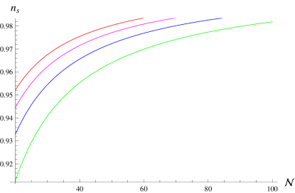
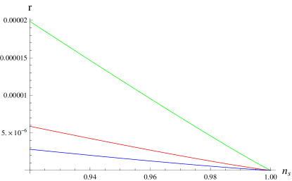
Figure 1: $n_{s}$ versus $\mathcal{N}$ (left) for $n=0.75$ (green), $n=1.1$ (blue), $n=1.5$ (magenta) and $n=1.98$ (red) whereas $r$ versus $n_{s}$ (right) for $n=0.9,~{}m=0.3$ (green), $n=0.8,~{}m=0.5$ (blue) and $n=0.75,~{}m=0.8$ (red).

$$V(\phi) = \frac{\chi_{1}}{(\frac{2n}{3n-1})}(-\phi)^{\frac{2n}{3n-1}},$$

$$H(t) = \left[\left(\frac{\chi_{1}(3n-1)}{2n}\right)\left(\frac{4\kappa^{2}(m+2)^{2}}{12^{n}f_{0}\{2(1-n)(m+2)^{2}+3n(2m+1)\}}\right)\right]^{\frac{1}{2n}}$$

$$\times (-\phi)^{\frac{1}{3n-1}},$$

where $\chi_{1}$ is constant given as

$$\chi_{1} = \left[\left\{\sqrt{\frac{3}{2}}\gamma\left(\frac{4\kappa^{2}(m+2)^{2}}{12^{n}f_{0}\{2(1-n)(m+2)^{2}+3n(2m+1)\}}\right)^{\frac{1}{2n}}\right\}^{2n}\right.$$

$$\times \left.\left(\frac{3n-1}{2n}\right)^{1-n}\right]^{\frac{1}{3n-1}}.$$

Notice that $V(\phi)$ is linear for $n=1$. The slow-roll parameters, spectral index and tensor-scalar ratio are

$$\epsilon = \frac{1}{4n(N+1)},\quad\eta=2(1-n)\epsilon,\quad n_{s}=1-\frac{n+2}{2n(\mathcal{N}+1)},$$ (42)

$$\quad r = \frac{4\kappa^{2}}{3}\gamma^{1-\frac{1}{n}}\left(\frac{12^{n}f_{0}\{2(1-n)(m+2)^{2}+3n(2m+1)\}}{4\kappa^{2}(m+2)^{2}}\right)^{\frac{1}{n}}$$ (43)

$$\times \left(\frac{n+2}{2n(1-n_{s})}\right)^{-\frac{1+n}{2n}}.$$

In Figure 1, the left plot indicates that the e-folds start decreasing as $n$ increases whereas the right panel shows that tensor-scalar ratio is compatible for all considered values of $n$ and $m$. The consistent behavior of $r$ is shown in both plots of Figure 2.

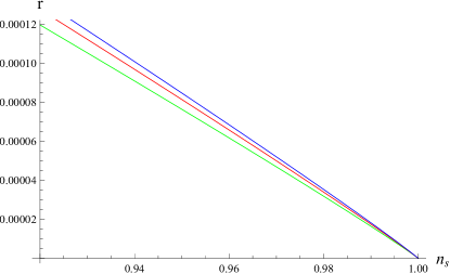
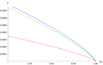
Figure 2: $r$ versus $n_{s}$ (left)$n=1.1,~{}m=0.3$ (green), $n=1.1,~{}m=0.5$ (blue) and $n=1.1,~{}m=0.8$ (red) while $r$ versus $n_{s}$ (right) for $n=1.8,~{}m=0.3$ (green), $n=1.92,~{}m=0.5$ (blue) and $n=1.98,~{}m=0.8$ (red).

When $\nu=\frac{1}{3}$, Eq.(29) becomes

$$\omega_{eff}=-1+\frac{1}{3}\left(\frac{\gamma}{\rho_{eff}}\right).$$ (44)

At the beginning of inflation, this effective parameter leads to the following from of inflaton field, potential and Hubble function as

$$\phi = \phi_{i}+\sqrt{\frac{\gamma}{3}}(t-t_{i}),\quad V(\phi)=\chi_{2}(1-\frac{1}{2n})(-\phi)^{\frac{1}{1-\frac{1}{2n}}},$$

$$H(t) = \left[\chi_{2}\left(1-\frac{1}{2n}\right)\left(\frac{4\kappa^{2}(m+2)^{2}}{12^{n}f_{0}\{2(1-n)(m+2)^{2}+3n(2m+1)\}}\right)\right]^{\frac{1}{2n}}$$

$$\times (-\phi)^{\frac{1}{2n(1-\frac{1}{2n})}},$$

where

$$\chi_{2}=\left[\left(1-\frac{1}{2n}\right)^{\frac{1}{2n}}(6\gamma)^{\frac{1}{2}}\left(\frac{4\kappa^{2}(m+2)^{2}}{12^{n}f_{0}\{2(1-n)(m+2)^{2}+3n(2m+1)\}}\right)^{\frac{1}{2n}}\right]^{\frac{1}{1-\frac{1}{2n}}},$$

and $V(\phi)$ called a generalized quadratic potential of chaotic inflation. The corresponding slow-roll parameters, spectral index and tensor-scalar ratio are

$$\epsilon = \frac{1}{2n(N+1)},\quad\eta=(2-n)\epsilon,\quad n_{s}=1-\frac{2}{n(\mathcal{N}+1)},$$ (45)

$$\quad r = \frac{8\kappa^{2}}{3}\gamma^{1-\frac{1}{n}}\left(\frac{12^{n}f_{0}\{2(1-n)(m+2)^{2}+3n(2m+1)\}}{4\kappa^{2}(m+2)^{2}}\right)^{\frac{1}{n}}$$ (46)

$$\times \left(\frac{2}{n(1-n_{s})}\right)^{-\frac{1}{n}}.$$

The left graph in Figure 3 describes that for quadratic potential, the e-folds are getting smaller as $n$ gets larger. The right plot shows that $r$ is consistent with Planck constraint whether we increase or decrease the value of anisotropy parameter whereas Figure 4 indicates the same results for $r$.

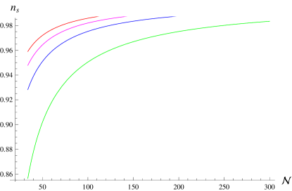
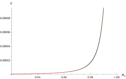
Figure 3: $n_{s}$ versus $\mathcal{N}$ (left) for $n=0.4$ (green), $n=0.8$ (blue), $n=1.1$ (magenta) and $n=1.4$ (red) and $r$ versus $n_{s}$ (right) for $n=0.4,~{}m=0.3$ (green), $n=0.4,~{}m=0.5$ (blue) and $n=0.4,~{}m=0.8$ (red).

For $\nu=\frac{2}{3}$, we have

$$\omega_{eff}=-1+\frac{2}{3}\left(\frac{\gamma}{\rho_{eff}}\right).$$ (47)

The scalar field and $H(t)$ can be expressed as

$$\phi = \phi_{i}+\sqrt{\frac{2\gamma}{3}}(t-t_{i}),\quad V(\phi)=\frac{\chi_{3}}{\frac{4n}{3n-2}}(-\phi)^{\frac{4n}{3n-2}},$$

$$H(t) = \left[\frac{\chi_{3}(3n-2)}{4n}\left(\frac{4\kappa^{2}(m+2)^{2}}{12^{n}f_{0}\{2(1-n)(m+2)^{2}+3n(2m+1)\}}\right)\right]^{\frac{1}{2n}}$$

$$\times (-\phi)^{\frac{2}{3n-2}}.$$

The potential of the scalar field corresponds to quartic potential model of chaotic inflation for $n=1$ with coupling constant given as

$$\chi_{3}=\left[\sqrt{6}\left(\frac{3n-2}{4n}\right)^{n+2}\gamma^{\frac{1}{4}}\left(\frac{4\kappa^{2}(m+2)^{2}}{12^{n}f_{0}\{2(1-n)(m+2)^{2}+3n(2m+1)\}}\right)^{\frac{1}{2n}}\right]^{\frac{4n}{3n-2}}.$$

In this case, the slow-roll and observational parameters become

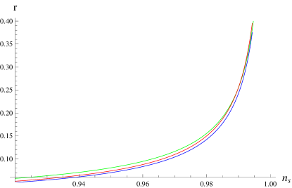
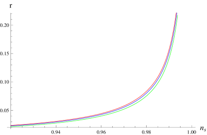
Figure 4: $r$ versus $n_{s}$ (left)$n=1.1,~{}m=0.3$ (green), $n=1.1,~{}m=0.5$ (blue) and $n=1.1,~{}m=0.8$ (red) while $r$ versus $n_{s}$ (right) for $n=1.4,~{}m=0.3$ (green), $n=1.3,~{}m=0.5$ (blue) and $n=1.3,~{}m=0.8$ (red).

$$\epsilon = \frac{1}{n(N+1)},\quad\eta=\frac{(4-n)\epsilon}{2},\quad n_{s}=1-\frac{4-n}{n(\mathcal{N}+1)},$$ (48)

$$\quad r = \frac{16\kappa^{2}}{3}\gamma^{1-\frac{1}{n}}\left(\frac{12^{n}f_{0}\{2(1-n)(m+2)^{2}+3n(2m+1)\}}{4\kappa^{2}(m+2)^{2}}\right)^{\frac{1}{n}}$$ (49)

$$\times \left(\frac{4-n}{n(1-n_{s})}\right)^{-1+\frac{2}{n}}.$$

In Figure 5, the left panel represents that there exists an inverse relation between $n$ and $\mathcal{N}$, i.e., e-folds decreases when $n$ increases and vice-versa. The best fit value of the e-folds is obtained for $n=1.5$ with quartic potential. The right plot indicates that we obtain a consistent range for $m=0.3,~{}0.5$ and $0.8$ whereas $n$ remains the same, i.e., $n=1.1$. Figures 6 and 7 yield a compatible range of tensor-scalar ratio for different values of $m$ and $n$.

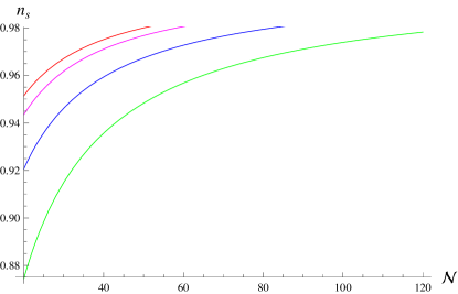
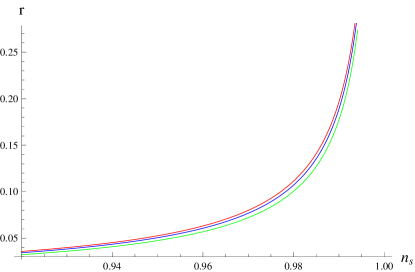
Figure 5: $n_{s}$ versus $\mathcal{N}$ (left) for $n=1.1$ (green), $n=1.5$ (blue), $n=1.83$ (magenta) and $n=1.98$ (red) and $r$ versus $n_{s}$ (right) for $n=1.1,~{}m=0.3$ (green), $n=1.1,~{}m=0.5$ (blue) and $n=1.1,~{}m=0.8$ (red).

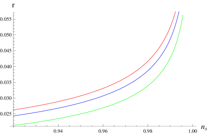
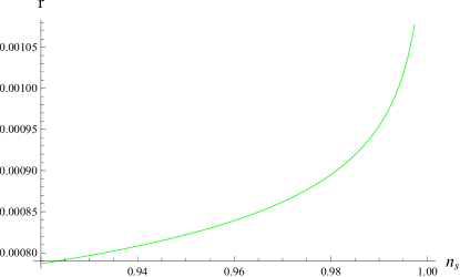
Figure 6: $r$ versus $n_{s}$ (left) for $n=1.5$, $m=0.3$ (green), $m=0.5$ (blue), $m=0.8$ (red) whereas $r$ versus $n_{s}$ (right) for $n=1.83,~{}m=0.3$ (green).

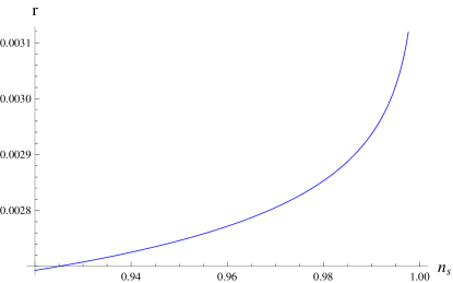
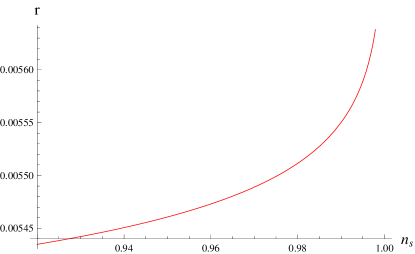
Figure 7: $r$ versus $n_{s}$ (left) for $n=1.92,~{}m=0.5$ (blue) while $r$ versus $n_{s}$ (right) for $n=1.98,~{}m=0.8$ (red).

3.2 Inflation via Fluid Cosmology

This is a well-known approach to any cosmological phenomenon which deals with perfect as well as imperfect fluid corresponding to ordinary radiation or matter in the universe. A straight forward description of rapid and uniform accelerated expansion of the universe is given by exotic matter which is governed by EoS different from radiation or ordinary matter. To discuss a graceful exit of rapid acceleration into a deceleration phase, quasi-de Sitter expansion in which EoS parameter depends on energy density. We consider the EoS parameter as

$$\omega(\tilde{\rho})=-1+\nu\left(\frac{\gamma}{\tilde{\rho}}\right)^{\frac{1}{3\nu}},$$ (50)

where $\tilde{\rho}$ and $\tilde{p}$ represent energy density and pressure of inhomogeneous fluid. The energy density from conservation law and Hubble parameter for $\nu=\frac{1}{6}$ are

$$\tilde{\rho} = \left[\mu_{0}-\gamma^{2}\left(\frac{4n-1}{12n}\right)\left(\frac{4\kappa^{2}(m+2)^{2}}{12^{n}f_{0}\{2(1-n)(m+2)^{2}+3n(2m+1)\}}\right)^{\frac{1}{2n}}\right.$$ (51)

$$\times \left.(t-t_{i})\right]^{\frac{2n}{4n-1}},$$

$$H = \left(\frac{4\kappa^{2}(m+2)^{2}}{12^{n}f_{0}\{2(1-n)(m+2)^{2}+3n(2m+1)\}}\right)^{\frac{1}{2n}}\left[\mu_{0}-\gamma^{2}\left(\frac{4n-1}{12n}\right)\right.$$ (52)

$$\times \left.\left(\frac{4\kappa^{2}(m+2)^{2}}{12^{n}f_{0}\{2(1-n)(m+2)^{2}+3n(2m+1)\}}\right)^{\frac{1}{2n}}(t-t_{i})\right]^{\frac{1}{4n-1}},$$

where $\mu_{0}$ is an integration constant of the quasi-de Sitter expansion. Inflation occurs when $t$ approaches to $t_{i}$ for which $\epsilon_{1}$ and $\epsilon_{2}$ become

$$\epsilon_{1}=\frac{1}{4n}\left(\frac{\gamma}{\tilde{\rho}}\right)^{2},\quad\epsilon_{2}=\left(\frac{\gamma}{\tilde{\rho}}\right)^{2}.$$

These parameters recover the expressions of slow-roll parameters, spectral index and tensor-scalar ratio when $\nu=\frac{1}{6}$ for the scalar field. Equations (17) and (50) lead to a relationship between number of e-folds and energy density of inhomogeneous fluid as

$$N+1=\left(\frac{\tilde{\rho}}{\gamma}\right)^{2}.$$

This provides a condition for the ending of inflation, i.e., $(\tilde{\rho}=\gamma)$ and scale factor takes the form

$$a(t)=a_{f}\exp\left[1-\left(\frac{\tilde{\rho}}{\gamma}\right)^{2}\right],$$

where $a_{f}$ denotes the scale factor at the end of inflation. For $\nu=\frac{1}{3}$, the energy density and Hubble parameter become

$$\tilde{\rho} = \left[\mu_{0}-\gamma\left(\frac{2n-1}{2n}\right)\left(\frac{4\kappa^{2}(m+2)^{2}}{12^{n}f_{0}\{2(1-n)(m+2)^{2}+3n(2m+1)\}}\right)^{\frac{1}{2n}}\right.$$ (53)

$$\times \left.(t-t_{i})\right]^{\frac{2n}{2n-1}},$$

$$H = \left(\frac{4\kappa^{2}(m+2)^{2}}{12^{n}f_{0}\{2(1-n)(m+2)^{2}+3n(2m+1)\}}\right)^{\frac{1}{2n}}\left[\mu_{0}-\gamma\left(\frac{2n-1}{2n}\right)\right.$$ (54)

$$\times \left.\left(\frac{4\kappa^{2}(m+2)^{2}}{12^{n}f_{0}\{2(1-n)(m+2)^{2}+3n(2m+1)\}}\right)^{\frac{1}{2n}}(t-t_{i})\right]^{\frac{1}{2n-1}}.$$

Using Eqs.(53) and (54), we obtain Hubble flow functions at $t=t_{i}$ as

$$\epsilon_{1}=\frac{1}{2n}\left(\frac{\gamma}{\tilde{\rho}}\right),\quad\epsilon_{2}=\left(\frac{\gamma}{\tilde{\rho}}\right).$$

The resulting slow-roll parameters, spectral index and tensor-scalar ratio turn out to be the same as for $\nu=\frac{1}{3}$ in the scalar field. The scale factor becomes

$$a(t)=a_{f}\exp\left[1-\left(\frac{\tilde{\rho}}{\gamma}\right)\right],$$

where $N+1=\frac{\tilde{\rho}}{\gamma}$. When $\nu=\frac{2}{3}$, the energy density, Hubble parameter and its flow functions for inhomogeneous fluid are

$$\tilde{\rho} = \left[\mu_{0}-\gamma^{\frac{1}{2}}\left(\frac{n-1}{n}\right)\left(\frac{4\kappa^{2}(m+2)^{2}}{12^{n}f_{0}\{2(1-n)(m+2)^{2}+3n(2m+1)\}}\right)^{\frac{1}{2n}}\right.$$ (55)

$$\times \left.(t-t_{i})\right]^{\frac{2n}{n-1}},$$

$$H = \left(\frac{4\kappa^{2}(m+2)^{2}}{12^{n}f_{0}\{2(1-n)(m+2)^{2}+3n(2m+1)\}}\right)^{\frac{1}{2n}}\left[\mu_{0}-\gamma^{\frac{1}{2}}\left(\frac{n-1}{n}\right)\right.$$ (56)

$$\times \left.\left(\frac{4\kappa^{2}(m+2)^{2}}{12^{n}f_{0}\{2(1-n)(m+2)^{2}+3n(2m+1)\}}\right)^{\frac{1}{2n}}(t-t_{i})\right]^{\frac{1}{n-1}},$$

$$\epsilon_{1} = \frac{1}{n}\left(\frac{\gamma}{\tilde{\rho}}\right),\quad\epsilon_{2}=\left(\frac{\gamma}{\tilde{\rho}}\right)^{\frac{1}{2}}.$$

The parameters $\epsilon_{1}$ and $\epsilon_{2}$ recover the slow-roll and observational parameters formulated for $\nu=\frac{2}{3}$ with scalar field.

Finally, we take EoS for $\nu=\frac{1}{3}$ and use the field equations (4) and (5) which yield

$$2\ddot{f}_{R}-6H\dot{f}_{R}\left[1-2\left(\frac{2m+1}{(m+2)^{2}}\right)\right]+12\dot{H}\left(\frac{2m+1}{(m+2)^{2}}\right)=-\frac{2\kappa^{2}\gamma}{3}.$$ (57)

The Hubble parameter and its derivative take the form

$$H=\sqrt{\frac{\kappa^{2}\gamma(m+2)^{2}(N+1)}{9(2m+1)}},\quad\dot{H}=\frac{\kappa^{2}\gamma(m+2)^{2}}{18(2m+1)},$$

which can also expressed in terms of e-folds at the end of inflation as

$$\frac{dH}{dN}=\frac{1}{2}\sqrt{\frac{\kappa^{2}\gamma(m+2)^{2}}{9(2m+1)(N+1)}}.$$

Thus, we can reconstruct $f(R)$ model by inserting the above derivative in Eq.(57) leading to

$$\frac{a(N+1)}{3}\ddot{f}_{R}+a\dot{f}_{R}\left[\frac{1}{6}+(N+1)\left(1-\frac{2}{a}\right)\right]-f_{R}=-1,$$

where $a=\frac{(m+2)^{2}}{2m+1}$. Integrating the above equation, we obtain

$$f_{R}(R) = \sqrt{N+1}\exp\left(-\frac{3(a-2)N}{a}\right)\left[c_{1}U\left(-\frac{1-a}{a-2},\frac{3}{2},\frac{3(a-2)(N+1)}{a}\right)\right.$$ (58)

$$+ \left.c_{2}L_{\frac{1-a}{a-2}}^{\frac{1}{2}}\left(\frac{3(a-2)(N+1)}{a}\right)\right]+1.$$

Here, $c_{1}$ and $c_{2}$ are integration constants whereas $U$ represents confluent hypergeometric function and $L$ denotes associated Laguerre polynomial. This equation (58) can also be expressed in terms of $R$ by taking

$$R=\kappa^{2}\gamma(4N+3),\quad N=\frac{3}{4}\left(\frac{(2m+1)R}{(m+2)^{2}\kappa^{2}\gamma}-1\right),$$ (59)

which implies that

$$f_{R}(R) = 1+\frac{1}{2}\sqrt{\frac{3R}{a\kappa^{2}\gamma}+1}\exp\left(\frac{-9(a-2)}{4a}\left(\frac{R}{a\kappa^{2}\gamma}-1\right)\right)$$

$$\times \left[c_{1}U\left(-\frac{1-a}{a-2},\frac{3}{2},\frac{9(a-2)}{4a}\left(\frac{R}{\kappa^{2}a\gamma}+1\right)\right)\right.$$

$$+ \left.c_{2}L^{\frac{1}{2}}_{\frac{1-a}{a-2}}\left(\frac{9(a-2)}{4a}\left(\frac{R}{a\kappa^{2}\gamma+1}\right)\right)\right].$$

Its integration leads to

$$f(R) = R+\frac{1}{2}\int\sqrt{\frac{3R}{a\kappa^{2}\gamma}+1}\exp\left(\frac{-9(a-2)}{4a}\left(\frac{R}{a\kappa^{2}\gamma}-1\right)\right)$$

$$\times \left[c_{1}U\left(-\frac{1-a}{a-2},\frac{3}{2},\frac{9(a-2)}{4a}\left(\frac{R}{\kappa^{2}a\gamma}+1\right)\right)\right.$$

$$+ \left.c_{2}L^{\frac{1}{2}}_{\frac{1-a}{a-2}}\left(\frac{9(a-2)}{4a}\left(\frac{R}{a\kappa^{2}\gamma+1}\right)\right)\right]+c_{3},$$

where $c_{3}$ is an integration constant. This $f(R)$ model corresponds to Starobinsky inflationary model for $n,~{}m,~{}f_{0}=1$.

4 Inflationary Model for $\mu\neq 1$

Here, we would like to investigate the existence of the viable inflationary models for $\mu=2$ with spectral index and tensor-scalar ratio given in Eqs.(24) and (27). In this case, the EoS (15) and Hubble flow functions (19) reduce to

$$\omega_{eff} = -1+\left(\frac{1}{9\nu}\right)\log^{2}\left[\frac{\rho_{eff}}{p_{eff}}\right],$$ (61)

$$\epsilon_{1} = \frac{3\nu}{2n(N+1)^{2}},\quad\epsilon_{2}=\frac{2}{(N+1)},$$ (62)

where $\epsilon_{2}$ is much larger than $\epsilon_{1}$. The observational parameters $(n_{s},~{}r)$ become

$$n_{s} = 1-\frac{2}{(\mathcal{N}+1)},$$ (63)

$$r = 2\kappa^{2}\nu\gamma^{1-\frac{1}{2n}}(1-n_{s})^{2}\left(\frac{12^{n}f_{0}\{2(1-n)(m+2)^{2}+3n(2m+1)\}}{4\kappa^{2}(m+2)^{2}}\right)^{\frac{1}{n}}$$ (64)

$$\times \exp\left[-\frac{3\nu(1-n_{s})(n-1)}{2n}\right],$$

where $(\mathcal{N}+1)^{2}=\frac{4}{(1-n_{s})^{2}}$. In this case, tensor-scalar ratio is found to be inconsistent with Planck constraint whereas $\mathcal{N}=59$.

For the inflation via scalar field, the kinetic energy and potential function for $n=1,~{}2,~{}3$ are formulated using Eqs.(32), (38) and (61) as

$$\dot{\phi} \simeq \frac{1}{3}\sqrt{\frac{V(\phi)}{\nu}}\left(\frac{\gamma}{V(\phi)-1}\right),$$ (65)

$$V(\phi) = 2\gamma^{\prime}\left\{c_{4}-\sqrt{\frac{2}{\nu}}\left(\frac{4\kappa^{2}(m+2)^{2}}{12f_{0}\{3(2m+1)\}}\right)^{\frac{1}{2}}\phi\right\},$$

$$V(\phi) = \left[\frac{5\gamma^{\prime}}{2}\left\{c_{4}-\sqrt{\frac{2}{\nu}}\left(\frac{4\kappa^{2}(m+2)^{2}}{144f_{0}\{-2(m+2)^{2}+6(2m+1)\}}\right)^{\frac{1}{4}}\phi\right\}\right]^{\frac{4}{5}},$$

$$V(\phi) = \left[\frac{8\gamma^{\prime}}{3}\left\{c_{4}-\sqrt{\frac{2}{\nu}}\left(\frac{4\kappa^{2}(m+2)^{2}}{12^{3}f_{0}\{-4(m+2)^{2}+9(2m+1)\}}\right)^{\frac{1}{6}}\phi\right\}\right]^{\frac{3}{4}},$$

where $c_{4}$ and $\gamma^{\prime}$ are integration constants. The above forms of potentials define massless large inflaton field in terms of fractional potential models that can be generalized as

$$\left\{c_{4}-\sqrt{\frac{2}{\nu}}\left(\frac{4\kappa^{2}(m+2)^{2}}{12^{n}f_{0}\{2(1-n)(m+2)^{2}+3n(2m+1)\}}\right)^{\frac{1}{2n}}\phi\right\}\frac{\gamma^{\prime}(3n-1)}{n}$$

$$=V^{\frac{3n-1}{2n}}(\phi)\left\{1+\left(\frac{3n-1}{5n-1}\right)\frac{V(\phi)}{\gamma^{\prime}}\right\}.$$

The fractional potential function corresponds to Starobinsky model for $m,~{}n=1$ (Starobinsky 1980). The slow-roll and observational parameters for $c_{4}=2,~{}\nu=\frac{1}{2}$ become

$$\epsilon = \frac{3}{4n(N+1)^{2}},\quad\eta=-\frac{1}{(N+1)}+\frac{3}{2n(N+1)^{2}},$$ (66)

$$\quad n_{s} = 1-\frac{2}{\mathcal{N}+1},$$ (67)

$$r = \kappa^{2}\gamma^{1-\frac{1}{2n}}(1-n_{s})^{2}\left(\frac{12^{n}f_{0}\{2(1-n)(m+2)^{2}+3n(2m+1)\}}{4\kappa^{2}(m+2)^{2}}\right)^{\frac{1}{n}}$$ (68)

$$\times \exp\left[-\frac{3(n-1)(1-n_{s})}{4n}\right].$$

In order to discuss inflation via fluid cosmology, we take inhomogeneous fluid so that EoS takes the form

$$\omega(\tilde{\rho})=-1+\frac{1}{9\nu}\log^{2}\left(\frac{\tilde{\rho}}{\gamma}\right).$$ (69)

Inserting Eq.(12) in the conservation law, we obtain

$$\tilde{\rho} = \gamma\left[1-\left(\frac{12^{n}f_{0}\{2(1-n)(m+2)^{2}+3n(2m+1)\}}{4\kappa^{2}(m+2)^{2}}\right)^{\frac{1}{2n}}\frac{3\nu}{\gamma^{\frac{1}{2n}}(t_{f}-t)}\right],$$

$$H = \left[1-3\nu\left(\frac{12^{n}f_{0}\{2(1-n)(m+2)^{2}+3n(2m+1)\}}{4\kappa^{2}(m+2)^{2}}\right)^{\frac{1}{2n}}\frac{1}{\gamma^{\frac{1}{2n}}(t_{f}-t)}\right]^{\frac{1}{2n}}$$ (71)

$$\times \left(\frac{4\kappa^{2}(m+2)^{2}}{12^{n}f_{0}\{2(1-n)(m+2)^{2}+3n(2m+1)\}}\right)^{\frac{1}{2n}}\gamma^{\frac{1}{2n}}.$$

In this limit $t<<t_{e}$, the Hubble parameter become

$$\epsilon_{1} = \frac{3\nu}{2n\gamma^{\frac{1}{n}}(t_{f}-t)^{2}}\left(\frac{12^{n}f_{0}\{2(1-n)(m+2)^{2}+3n(2m+1)\}}{4\kappa^{2}(m+2)^{2}}\right)^{\frac{1}{n}},$$ (72)

$$\epsilon_{2} = \frac{2}{\gamma^{\frac{1}{2n}}(t_{f}-t)}\left(\frac{12^{n}f_{0}\{2(1-n)(m+2)^{2}+3n(2m+1)\}}{4\kappa^{2}(m+2)^{2}}\right)^{\frac{1}{2n}}.$$ (73)

To describe the duration of inflation, the number of e-folds and scale factor turn out to be

$$N = \left(\frac{4\kappa^{2}(m+2)^{2}\gamma}{12^{n}f_{0}\{2(1-n)(m+2)^{2}+3n(2m+1)\}}\right)^{\frac{1}{2n}}(t_{f}-t)-1,$$

$$a(t) = a_{f}\exp\left[1-\left(\frac{4\gamma\kappa^{2}(m+2)^{2}}{12^{n}f_{0}\{2(1-n)(m+2)^{2}+3n(2m+1)\}}\right)^{\frac{1}{2n}}(t-t_{f})\right].$$

The parameters $\epsilon_{1}$ and $\epsilon_{2}$ recover the expressions given in Eqs.(62)-(64).

5 Concluding Remarks

This paper is devoted to study inflation via two approaches scalar field and fluid cosmology in $f(R)$ gravity using LRS BI universe model. When the inflaton field starts from a large field value and then rolls down towards the minimum value of potential function, the field value is about to vanish at this point. This is known as chaotic inflation in which inflaton field is greater than $M_{Pl}$ and ends when inflaton field is nearly close to $M_{Pl}$. Models which correspond to chaotic inflation are known as large field models. To investigate such type of inflation, we have taken EoS with a deviation parameter which describes quasi-de Sitter expansion and leads to an elegant exit from inflation to deceleration phase. We have furnished some basic features of inflation and formulated Hubble flow functions as well as slow-roll parameters in fluid cosmology and scalar field for a power-law model of $f(R)$ gravity.

We have analyzed inflation by taking different values of $\nu$ with $\mu=1$ and $\mu\neq 1$. We have calculated slow-roll parameters, spectral index and tensor-scalar ratio for all these values. The results can be summarized as follows.

• For $\nu=\frac{1}{6}$, we have constructed the graphical analysis for $m=0.3,~{}0.5,~{}0.8$ and $n=0.9,~{}0.8,~{}0.75$. The tensor-scalar ratio $r$ shows consistency with Planck observations for $n=0.75$ with $m\geq-0.69,~{}m\geq-12.31$ and $m>0$ ($m\neq 1,~{}2$) whereas for $-0.7\leq{m}\leq-12.3$, there is no graphical interpretation. For $n=1.98$, we have obtained consistent results for $0.727\leq{m}\leq 1.335$. The compatible number of e-folds are $\mathcal{N}=54,~{}\mathcal{N}=41,~{}\mathcal{N}=34,~{}\mathcal{N}=29$ for $n=0.7,~{}1.1,~{}1.5,~{}1.98$, respectively. We have found consistent results as e-folds as well as anisotropic parameter are getting smaller when $n$ is getting larger.

• In case of $\nu=\frac{1}{3}$, the range of $n$ is $0.4\leq{n}\leq 1.4,~{}0.4\leq{n}\leq 1.3,~{}0.4\leq{n}\leq 1.3$ for the above values of anisotropic parameter. For $n=0.4,~{}0.8,~{}1.1$ and $1.4$, the e-folds are found to be $\mathcal{N}=148,~{}\mathcal{N}=74,~{}\mathcal{N}=53$ and $\mathcal{N}=29$, respectively. The tensor-scalar ratio is compatible with recent observational data for $n=0.4$ with all values of $m$ instead of $-1\leq{m}\leq-5,~{}(m\neq 0,~{}1,~{}2)$. When $n=1.6$, the results are found to be consistent for $0<m\leq 0.2$.

• When $\nu=\frac{2}{3}$, the range of $n$ becomes $1.1\leq{n}\leq 1.83,~{}1.1\leq{n}\leq 1.92,~{}1.1\leq{n}\leq 1.98$ for the same anisotropy values. The e-folds gives $\mathcal{N}=78,~{}49,~{}34,~{}30$ for $n=1.1,~{}1.5,~{}1.83$ and $1.98$, respectively. The tensor-scalar ratio turns out to be compatible with Planck constraint for $n=1.1$ and $n=1.98$ with $-0.42\leq{m}\leq 29.4$ and $0.727\leq{m}\leq 1.335$, respectively.

In fluid cosmology, we have calculated Hubble flow functions $(\epsilon_{1},~{}\epsilon_{2})$ which recover expressions of the spectral index and tensor-scalar ratio for the scalar field. We have also evaluated the value of $f(R)$ which corresponds to Starobinsky inflationary model for $n,~{}f_{0},~{}m=1$. For $\mu\neq 1$, we have taken $\mu=2$ and constructed observational parameters for $\nu$ and expressions found in fluid cosmology. We again recover these observational parameters as well as Hubble flow functions. We have investigated inflation with scalar field and developed expressions of kinetic and potential functions. In this case, the tensor-scalar ratio is incompatible to Planck constraints whereas $\mathcal{N}=59$ for all values of $n$ and $\nu$.

Myrzakulov et al. (2015) analyzed the dynamics of inflation via scalar field as well as fluid cosmology through isotropic homogeneous universe model in $f(R)$ gravity. To explore the existence of inflationary epoch with smooth ending, they considered quasi-de Sitter expansion with the EoS parameter evolving e-folds. In the scalar field representation, they obtained quadratic form of potential function compatible with massive scalar field. They also claimed that for $\mu=2$, the amount of e-folds as well as tensor-scalar ratio is found to be consistent with recent Planck’s constraints whereas this ratio appears to be larger for $\mu=1$. In the presence of inhomogeneous fluids, they determined explicit solutions which preserve the same behavior as scalar field to produce inflation. In this paper, we have found consistent range of e-folds as well as tensor-scalar ratio relative to different ranges of anisotropic parameter and for all considered values of $\nu$ whereas in case of $\mu=2$, the tensor-scalar ratio exceeds from Planck’s suggested limit. We have also found expressions of kinetic and potential energies for scalar field with $\nu=\frac{1}{6},~{}\frac{1}{3}$ and $\frac{2}{3}$ which yield linear, quadratic and quartic potential models, respectively. In case of inhomogeneous fluid, the density dependent EoS parameter identifies the same behavior of observational parameters as in the presence of scalar field. It is worth mentioning here that all our results are consistent with isotropic and homogeneous universe for $n,~{}m,~{}f_{0}=1$ (Myrzakulov et al. 2015).

Acknowledgments

This work has been supported by the Pakistan Academy of Sciences Project.

References

- [1] Ade, P.A.R. et al.: Astron. Astrophys. 594, A20(2016)
- [2] Albrecht, A. and Steinhardt, P.: Phys. Rev. Lett. 48, 1220(1982)
- [3] Akarsu, Ö. and Kilinc, C.B.: Astrophys. Space Sci. 326, 315(2010)
- [4] Artymowski, M. and Lalak, Z.: J. Cosmo. Astropart. Phys. 09, 036(2014)
- [5] Mukhanov, V.: Physical Foundations of Cosmology, Cambridge University Press, (2005)
- [6] Bamba, K., Nojiri, S., Odintsov, S.D. and Sáez-Gómez, D.: Phys. Rev. D 90, 124061(2014)
- [7] Bamba, K. and Odintsov, S.D.: Symmetry 7, 220(2015)
- [8] Bamba, K. and Odintsov, S.D.: Eur. Phys. J. C 76, 18(2016)
- [9] Barrow, J.D. and Turner, M.S.: Nature 292, 35(1982)
- [10] Chung, D.J.H., Kolb, E.W. and Riotto, A.: Phys. Rev. Lett. 81, 4048(1998)
- [11] Collins, C.B., Glass, E.N. and Wilkinson, D.A.: Gen. Relativ. Gravit. 12, 805(1980)
- [12] Gao, X., Li, T. and Shukla, P.: Phys. Lett. B 738, 412(2014)
- [13] Guth, A. H.: Phys. Rev. D 23, 347(1981)
- [14] Huang, Q.G.: J. Cosmo. Astropart. Phys. 02, 035(2014)
- [15] Hussain, I., Jamil, M. and Mahomed, F.M.: Astrophys. Space Sci. 337, 373(2012)
- [16] Kofman, L., Linde, A. and Starobinsky, A.A.: Phys. Rev. Lett. 73, 3185(1994)
- [17] Linde, A.: Phys. Lett. B 129, 177(1983)
- [18] Linde, A.: Particle Physics and Inflationary Cosmology, Harwood Academic, (1990)
- [19] Lyth, D.H. and Liddle, A.R.: The Primordial Density Perturbation: Cosmology, Inflation and the Origin of Structure, Cambridge University Press, (2009)
- [20] Maartens, R., Wands, D., Bassett, B.A. and Heard, I.P.C.: Phys. Rev. D 62, 041301(2000)
- [21] Mukhanov, V.: Eur. Phys. J. C 73, 2486(2013)
- [22] Myrzakulov, R., Sebastiani, L. and Zerbini, S.: Eur. Phys. J. C 75, 215(2015)
- [23] Myrzakul, S., Myrzakulov, R. and Sebastiani, L.: Eur. Phys. J. C 75, 111(2015)
- [24] Nojiri, S. and Odintsov, S.D.: Phys. Rev. D 72, 023003(2005)
- [25] Nojiri, S. and Odintsov S.D.: Phys. Rep. 505, 59(2011)
- [26] Sato, K.: Mon. Not. R. Aston. Soc. 195, 467(1981)
- [27] Sharif, M. and Saleem, R.: Eur. Phys. J. C 74, 2738(2014)
- [28] Sharif, M. and Saleem, R.: Astropart. Phys. 62, 100(2015)
- [29] Sharif, M. and Saleem, R.: Astropart. Phys. 62, 241(2015)
- [30] Sharif, M. and Nawazish, I.: Astrophys. Space Sci. 361, 19(2016)
- [31] Sharif, M. and Nawazish, I.: Astrophys. Space Sci. 362, 30(2017a)
- [32] Sharif, M. and Nawazish, I.: Int. J Mod. Phys. 26, 1750191(2017b)
- [33] Sharif, M. and Ikram, A.: Int. J. Mod. Phys. D 26, 1750030(2017)
- [34] Starobinsky, A.A.: Phys. Lett. B 91, 99(1980)
- [35]