RVB signatures in the spin dynamics of the square-lattice Heisenberg antiferromagnet

Abstract

We investigate the spin dynamics of the square-lattice spin-$\frac{1}{2}$ Heisenberg antiferromagnet by means of an improved mean field Schwinger boson calculation. By identifying both, the long range Néel and the RVB-like components of the ground state, we propose an educated guess for the mean field magnetic excitation consisting on a linear combination of local and bond spin flips to compute the dynamical structure factor. Our main result is that when this magnetic excitation is optimized in such a way that the corresponding sum rule is fulfilled, we recover the low and high energy spectral weight features of the experimental spectrum. In particular, the anomalous spectral weight depletion at $(\pi,0)$ found in recent inelastic neutron scattering experiments can be attributed to the interference of the triplet bond excitations of the RVB component of the ground state. We conclude that the Schwinger boson theory seems to be a good candidate to adequately interpret the dynamic properties of the square-lattice Heisenberg antiferromagnet.

1 Introduction

The nature of the spin excitations in two dimensional (2D) quantum antiferromagnets (AF) represents one of the major challenges in strongly correlated electron systems. Originally motivated by the cuprates superconductors [1], the square-lattice Heisenberg antiferromagnet has long been the prototypical model to investigate the validity of the spin wave [2] and the resonant valence bond (RVB) descriptions [3]. Here, in contrast to the one dimensional case [4, 5, 6, 7], the ground state has long range Néel order, so it is expected that spin-$1$ magnon excitations take correctly into account the low energy part of the spectrum [2]. However, due to the presence of strong quantum fluctuations, there is an increasing belief that the high energy part of the spectrum can be described by pairs of spin-$\frac{1}{2}$ spinons, representing the excitations of the isotropic component of the ground state [3].
Recent high resolution inelastic neutron scattering experiments performed in the metal organic compound $Cu(DCOO)_{2}\cdot 4D_{2}O$ (CFDT) –a known realization of the square-lattice Heisenberg AF model– seem to support this argument [8]. Specifically, the spectrum has i) well defined low energy magnon peaks around $(\pi,\pi)$; ii) a wipe out of the intensity along with a downward renormalization of the dispersion near $(\pi,0)$ and iii) the continuum excitation at $(\pi,0)$ is isotropic, in contrast to the $(\frac{\pi}{2},\frac{\pi}{2})$ one. Signals of these features were also found in the undoped cuprates, being their origin attributed to the possible presence of extra ring exchange interactions due to charge fluctuations effects [9]. In CFDT, however, the electrons are much more localized implying a negligible role of charge fluctuations [14]. In fact, the dispersion relation measured in CFDT has a deviation with respect to linear spin wave theory at $(\pi,0)$ but agrees very well with series expansion [10] and quantum Monte Carlo [11] calculations performed in the pure Heisenberg model. Furthermore, spin wave calculations reproduce the correct spectral weight of the spectrum around $(\pi,\pi)$ while the anomaly at $(\pi,0)$ seems to be reproduced by a Gutzwiller projected wave function calculation where the isotropic continuum is interpreted as spatially extended pairs of fermionic spinons [8]. This calculation, however, fails to consistently describe at the same time the low energy part of the spectrum near $(\pi,\pi)$.

On the other hand, recently, a whole description of the dispersion relation in terms of magnons was performed using a continuous similarity transformation [12]. In this context, the downward renormalization at $(\pi,0)$ was attributed to a significant spectral weight transfer from the single magnon states to the three magnon continuum. Unfortunately, the corresponding dynamical structure factor has not been computed; so a close comparison with the measured spectral weight has not been carried out yet.

Alternatively, two decades ago, Arovas and Auerbach developed a bosonic spinon-based theory [13]. Using a mean field Schwinger boson (MFSB) theory they computed the dynamical structure factor $S({\bf k},\omega)$ in the square-lattice antiferromagnet (see fig. 1(a)). Even if the spectrum shows a low energy dominant spectral weight around $(\pi,\pi)$ with a magnon dispersion that matches the spin wave result, the spectral weight at $(\pi,0)$ and $(\frac{\pi}{2},\frac{\pi}{2})$ are practically the same, namely, at odds with the experimental spectrum (see fig. 1(b)). In view of the recent neutron scattering experiments on CFDT, and the theoretical difficulties mentioned above, the search for a consistent theoretical description that takes into account the main features of the spectrum has become an important goal.

In this paper. we perform an improved mean field Schwinger boson calculation of the dynamical structure factor for the square-lattice Heisenberg antiferromagnet. Using the fact that the mean field ground state can be described by a Néel and an averaged RVB component, we investigate the corresponding spectral properties and propose an educated guess for the magnetic excitations consisting of a linear combination of local and bond spin flips. Notably, when this magnetic excitation is optimized in such a way that the sum rule $\int d\omega\sum_{\bf k}S({\bf k},\omega)=NS(S+1)$ is fulfilled we find that the main spectral weight features of the experimental spectrum are reproduced quite well (see fig. 3(a)). In particular, our results support the idea that the anomalous spectral weight depletion at $(\pi,0)$ can be attributed to the interference of the triplet bond excitations corresponding to the averaged RVB component of the ground state [14].

2 Néel and RVB components of the mean field Schwinger boson ground state

It is firmly established that the ground state of the spin-$\frac{1}{2}$ Heisenberg model on the square-lattice is an $SU(2)$ broken symmetry quantum Néel state [2]. Nonetheless, the nature of the zero point quantum fluctuations and the spin excitations above the ground state are still controversial. It has been proposed that the zero point quantum fluctuations have both local and RVB character, the latter being related to the anomaly found at $(\pi,0)$ in the neutron scattering experiments of CFDT [14]. In this section we show that the ground state provided by the MFSB can be related to the above proposal.

Here, we present the main steps of the mean field Schwinger boson theory, originally developed by Arovas and Auerbach[13]. Within the Schwinger boson representation the spin operators are expressed as ${\hat{\bf S}}_{i}\!\!=\!\frac{1}{2}{\bf b}^{\dagger}_{i}\vec{\sigma}\;{\bf b}_{i}$, with the spinor ${\bf b}^{\dagger}_{i}\!=\!(\hat{b}^{\dagger}_{i\uparrow};\hat{b}^{\dagger}_{i\downarrow})$ composed by the bosonic operators $\hat{b}^{\dagger}_{i\uparrow}$ and $\hat{b}^{\dagger}_{i\downarrow}$, and $\vec{\sigma}\!\!=\!\!(\sigma^{x},\sigma^{y},\sigma^{z})$ the Pauli matrices. To fulfill the spin algebra the constraint of $2S$ bosons per site, $\sum_{\sigma}\hat{b}^{\dagger}_{i\sigma}\hat{b}_{i\sigma}\!=2S$, must be imposed. Using this representation the AF Heisenberg Hamiltonian results [13],

$$\frac{J}{2}\sum_{<i,j>}\hat{\bf S}_{i}\!\cdot\!\hat{\bf S}_{j}=\frac{J}{2}\sum_{<i,j>}\left[S^{2}-2\hat{A}^{\dagger}_{ij}\hat{A}_{ij}\right],$$ (1)

where $J>0$ is the exchange interaction between nearest neighbors $<\!\!ij\!\!>$ and $\hat{A}^{\dagger}_{ij}\!=\!\frac{1}{2}\sum_{\sigma}\sigma\hat{b}^{\dagger}_{i\sigma}\hat{b}^{\dagger}_{j\bar{\sigma}}$ is a singlet bond operator [15]. Introducing a Lagrange multiplier $\lambda$ to impose the local constraint on average and performing a mean field decoupling of eq. (1), such that $A_{ij}=\langle\hat{A}_{ij}\rangle=\langle\hat{A}^{\dagger}_{ij}\rangle$, the diagonalized mean field Hamiltonian yields[13, 16, 18]

$$\hat{H}_{MF}=E_{\texttt{gs}}+\sum_{\bf k}\omega_{\bf k}\left[\hat{\alpha}^{\dagger}_{{\bf k}\uparrow}\hat{\alpha}_{{\bf k}\uparrow}+\hat{\alpha}^{\dagger}_{-{\bf k}\downarrow}\hat{\alpha}_{-{\bf k}\downarrow}\right],$$

where

$$E_{\texttt{gs}}=\sum_{\bf k}\omega_{\bf k}{-\frac{N}{2}\sum_{\delta}J(S^{2}-A^{2}_{\delta})}-\lambda N(2S+1)$$

is the ground state energy, with $A_{\delta}\!$ chosen real and $\delta$ connecting all the first neighbors of a square lattice, while

$$\omega_{{\bf k}\uparrow}=\omega_{{\bf k}\downarrow}=\omega_{\bf k}=[\lambda^{2}-(\gamma^{A}_{\bf k})^{2}]^{\frac{1}{2}},$$

is the spinon dispersion relation with $\gamma^{A}_{\bf k}\!\!=\!\!\frac{1}{2}J\sum_{\delta}A_{\delta}\sin({\bf k}.\delta)$, The ground state wave function $|\texttt{gs}\rangle$ is such that $\hat{\alpha}_{{\bf k}\uparrow}|\texttt{gs}\rangle=\hat{\alpha}_{{\bf k}\downarrow}|\texttt{gs}\rangle=0$ and has a Jastrow form [19]

$$|\texttt{gs}\rangle\;=e^{\sum_{\bf k}f_{\bf k}b^{\dagger}_{{\bf k}\uparrow}b^{\dagger}_{-{\bf k}\downarrow}}|0\rangle_{b},$$ (2)

where $|0\rangle_{b}$ is the vacuum of Schwinger bosons $b$ and $f_{\bf k}=-v_{\bf k}/u_{\bf k}$, with $u_{\bf k}\!=\![\frac{1}{2}(1+\frac{\lambda}{\omega_{\bf k}})]^{\frac{1}{2}}$ and $v_{\bf k}\!=\!\imath\ {\it sgn}(\gamma^{A}_{\bf k})[\frac{1}{2}(-1+\frac{\lambda}{\omega_{\bf k}})]^{\frac{1}{2}}$ the Bogoliubov coefficients used to diagonalize $\hat{H}_{MF}$. The self consistent mean field equations for $A_{\delta}\!$ and $\lambda$ are,

$$A_{\delta} = \frac{1}{2N}\sum_{\bf k}\frac{\gamma^{A}_{\bf k}}{\omega_{\bf k}}\sin({\bf k}.{\delta})$$ (3)

$$S+\frac{1}{2} = \frac{1}{2N}\sum_{\bf k}\frac{\lambda}{\omega_{\bf k}}.$$ (4)

The rotational invariance preserved by the MFSB allows us to study finite size systems directly, avoiding the singularities that arise when a broken symmetry state is assumed, like in spin wave theory [20]. Numerical computation of the above self consistent equations shows two gauge related singlet solutions, the $s$ wave ($A_{\delta_{x}}=A_{\delta_{y}}$) [13] and the $d$ wave ($A_{\delta_{x}}=-A_{\delta_{y}}$) [21] solutions. In particular, as soon as the system size $N$ increases, both solutions develop $180^{\circ}$ Néel correlations signaled by the minimum gap of the spinon dispersion at $\pm(\frac{\pi}{2},\frac{\pi}{2})$ that vanishes in the thermodynamic limit. This closing of the gap is related to the spontaneous $SU(2)$ broken symmetry Néel state [22, 19]. By the way, it is instructive to rearrange eq. (4) as

$$S=\frac{1}{N}\sum_{\bf k}\frac{|f_{\bf k}|^{2}}{[1-|f_{\bf k}|^{2}]}.$$ (5)

In the thermodynamic limit the self consistent solutions yield $|f_{\pm(\frac{\pi}{2},\frac{\pi}{2})}|\rightarrow 1$. Then, the quantum corrected magnetization $m$ can be obtained as the singular part of eq. (5) [19],

$$m=\frac{2}{N}\frac{|f_{(\frac{\pi}{2},\frac{\pi}{2})}|^{2}}{[1-|f_{(\frac{\pi}{2},\frac{\pi}{2})}|^{2}]}.$$ (6)

From eq. (2), it is clear that the singular behavior is due to the condensation of spin up and spin down bosons at ${\bf k}=\pm(\frac{\pi}{2},\frac{\pi}{2})$. Consequently, in the thermodynamic limit, the ground state can be splitted as

$$|\texttt{gs}\rangle\;=|\texttt{c}\rangle|\texttt{n}\rangle,$$

where

$$|\texttt{c}\rangle=e^{{{\sqrt{\frac{Nm}{2}}}}\left({b}^{\dagger}_{(\frac{\pi}{2},\frac{\pi}{2})\uparrow}+{b}^{\dagger}_{-(\frac{\pi}{2},\frac{\pi}{2})\uparrow}+i{b}^{\dagger}_{(\frac{\pi}{2},\frac{\pi}{2})\downarrow}-i{b}^{\dagger}_{-(\frac{\pi}{2},\frac{\pi}{2})\downarrow}\right)}|0\rangle_{b}\\$$ (7)

is the condensate part which represents the quantum corrected Néel state, $\langle\texttt{C}|S^{z}_{\bf r}|\texttt{C}\rangle=(-1)^{r_{x}+r_{y}}m$, and

$$|\texttt{n}\rangle\;=e^{\small{\sum_{\small{{\bf k}\neq\pm(\frac{\pi}{2},\frac{\pi}{2})}}f_{\bf k}b^{\dagger}_{{\bf k}\uparrow}b^{\dagger}_{-{\bf k}\downarrow}}}|0\rangle_{b}$$

is the isotropic normal fluid part which represents the zero point quantum fluctuations of the ground state [19]. A practical advantage of the MFSB theory is that, even working on finite systems, it is possible to keep track of the putative magnetic order. For instance, a finite size scaling of eq. (6) gives $m=0.3034$, in agreement with Arovas and Auerbach result [13]. Going back to real space the normal fluid part is, approximately,

$$|\texttt{n}\rangle\;\approx e^{\sum_{ij}f_{ij}\hat{A}^{\dagger}_{ij}}|0\rangle_{b},$$ (8)

where $f_{ij}$ is the Fourier transform of $f_{\bf k}$. Equation (8) shows explicitly the singlet bond structure of the normal fluid part of the ground state. Although it is not a true RVB state, because the constraint is only satisfied on average, one can still interpret the normal fluid component of the ground state as an averaged RVB component.

Keeping in mind this picture for the ground state, two kind of magnetic excitations can be envisaged within the MFSB: local spin flips and bond spin flips acting on the condensate and normal fluid components, respectively. On one hand, magnonic-like excitations are created by $\hat{S}{{}^{z}}_{\bf q}$, which is a linear combination of the local operator $\hat{S}{{}^{z}}_{i}$. On the other hand, triplet bond excitations of the averaged RVB component can be created by $D^{\dagger}_{\bf q}$, which is a linear combination of the bond operator

$$\hat{D}^{\dagger}_{i}=\frac{1}{2}(D^{\dagger}_{i\delta_{x}}+D^{\dagger}_{i\delta_{y}}),$$

with

$$D^{\dagger}_{i\delta}=b^{\dagger}_{i\uparrow}b^{\dagger}_{i+\delta\downarrow}+b^{\dagger}_{i\downarrow}b^{\dagger}_{i+\delta\uparrow}$$

that creates a triplet of $z-$component equal to zero; while operators like $T^{\dagger}_{i\delta\uparrow}=b^{\dagger}_{i\uparrow}b^{\dagger}_{i+\delta\uparrow}$ and $T^{\dagger}_{i\delta\downarrow}=b^{\dagger}_{i\downarrow}b^{\dagger}_{i+\delta\downarrow}$ create triplets of $z-$component equal to $\pm 1$, respectively. Actually, other kind of triplet bond excitations such as $C^{\dagger}_{i\delta}=b^{\dagger}_{i\uparrow}b_{i+\delta\uparrow}-b^{\dagger}_{i\downarrow}b_{i+\delta\downarrow}$, can be constructed. However, after a systematic study of all possible triplet bond excitations we have found that the correct spectral properties are recovered once the excitations corresponding to $D^{\dagger}_{i\delta}$, $T^{\dagger}_{i\delta\uparrow}$, and $T^{\dagger}_{i\delta\downarrow}$ are incorporated in the dynamical structure factor calculation (see below).

3 Dynamical structure factor study

In this section we show the difficulty of the original MFSB theory [13] to recover the anomaly of the spectrum at $(\pi,0)$ and we propose an improved calculation of the dynamical structure factor by considering, explicitly, the triplet bond excitations $\hat{D}^{\dagger}_{\bf q}$ mentioned in the previous section. At zero temperature the dynamical structure factor is defined as

$$S({\bf k},\omega)=\sum_{n}|\langle\texttt{gs}|\hat{\bf S}_{\bf k}|n\rangle|^{2}\delta(\omega-(\epsilon_{n}-E_{\texttt{gs}})),$$

where $|n\rangle$ are the spin-$1$ excited states. Plugging the corresponding mean field states in eq. (3) results in

$$S({\bf k},\omega)\!=\!\frac{1}{4N}\!\!\sum_{{\bf q}}|u_{{\bf k}+{\bf q}}v_{\bf q}-u_{{\bf q}}v_{{\bf k}+{\bf q}}|^{2}\delta(\omega-(\omega_{-{\bf q}}+\omega_{{\bf k}+{\bf q}})).$$ (9)

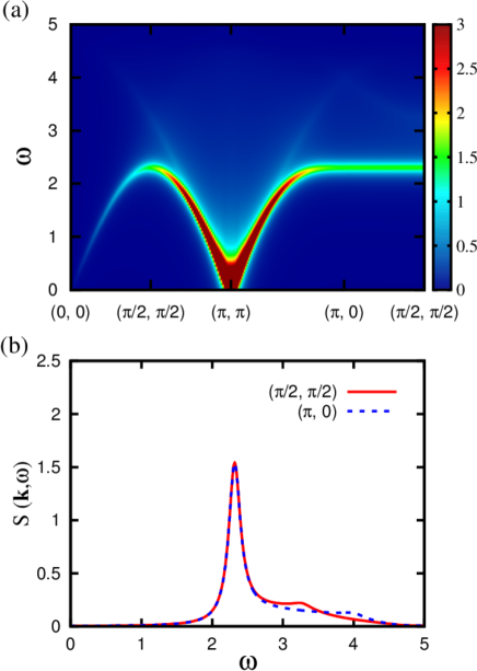
Figure 1: Dynamical structure factor $S({\bf k},\omega)$ within the MFSB (eq. (9)). (a) intensity curve along a path of the Brillouin zone. (b) comparison between ${\bf k}=(\frac{\pi}{2},\frac{\pi}{2})$ (solid line) and ${\bf k}=(\pi,0)$ (dashed line).

By exploiting the fact that the MFSB theory fulfills the Mermin Wagner theorem[23], Arovas and Auerbach accessed to the above zero temperature dynamical structure factor coming from the finite temperature regime [13]. Here, instead, we work at zero temperature and use finite size systems to compute eq. (9) where the contribution of the $x,y$ and $z$ components are identical due to the $SU(2)$ symmetry of the ground state. However, due to the development of long range Néel order, the spectrum shows Bragg peaks and low energy Goldstone modes at ${\bf k}=(0,0)$ and $(\pi,\pi)$. This is shown in fig. 1(a) where eq. (9) is displayed in an intensity curve. Even if the spectrum is expressed in terms of free pairs of spinons it is expected that gauge fluctuations, dynamically generated, will confine them into magnonic excitation [24, 25]. In fact, a simple first order calculation in perturbation theory supports the picture of tightly bond pair of spinons in the neighborhood of the Goldstone modes [26]. Furthermore, the spectrum shows a low energy dominant spectral weight around $(\pi,\pi)$ with a magnon dispersion that matches the spin wave result. However the spectral weight at $(\pi,0)$ and $(\frac{\pi}{2},\frac{\pi}{2})$ are practically the same (see fig. 1(b)), that is, at odds with the anomaly observed at $(\pi,0)$ in the neutron scattering experiments of CFDT [8]. This anomaly was previously interpreted as a quantum mechanical interference due to the entanglement of the RVB component of the ground state [14]. This motivated us to focus on the spectral properties of the triplet bond operator $D^{\dagger}_{i}$ which, within the context of our approximation, represents a proper magnetic excitation of the averaged RVB component of the mean field ground state. The corresponding dynamical structure factor is

$$D({\bf k},\omega)=\sum_{n}|\langle\texttt{gs}|\hat{D}_{\bf k}|n\rangle|^{2}\delta(\omega-(\epsilon_{n}-E_{\texttt{gs}})),$$

with $\hat{D}_{\bf k}$ the Fourier transform of $D^{\dagger}_{i}$. Within the MFSB eq. (3) results

$$D({\bf k},\omega)\!=\!\frac{1}{N}\!\sum_{\bf q}[\left(\gamma_{\bf k}+\gamma_{\bf k+q}\right)u_{\bf k}u_{\bf k+q}]^{2}\delta\!\left(\omega-\omega_{\bf k}-\omega_{\bf k+q}\right)$$ (10)

with $\gamma_{\bf k}\!=\!\frac{1}{2}\sum_{\delta}\cos{\bf k}.\delta$. In fig. 2(a) is plotted eq. (10) in an intensity curve. As expected, the spectral weight of these triplet bond fluctuations is mostly located at high energies. Notice the high energy spectral weight transfer with respect to $S({\bf k},\omega)$ (see fig. 1(a)). In particular, at $(\pi,0)$ the spectral weight transfer is complete (see fig. 2(b)). It is important to note that among all possible triplet bond excitations mentioned in the previous section only the spectrum of $D({\bf q},\omega)$ shows this interference at $(\pi,0)$.

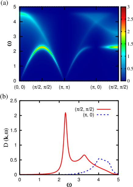
Figure 2: Dynamical structure factor $D({\bf k},\omega)$ within the MFSB (eq. (10)). (a) intensity curve along a path of the Brillouin zone. (b) comparison between ${\bf k}=(\frac{\pi}{2},\frac{\pi}{2})$ (solid line) and ${\bf k}=(\pi,0)$ (dashed line).

In principle, such anomaly should appear in a rigorous calculation of $S({\bf k},\omega)$. But it is known that, due to the relaxation of the local constraint, the excitations created by $\hat{S}_{\bf q}$ in the MFSB are not completely physical, producing a factor $\frac{3}{2}$ in the sum rule, $\int d\omega\sum_{\bf k}S({\bf k},\omega)=\frac{3}{2}NS(S+1)$ [13]. Therefore, to improve the $S({\bf k},\omega)$ calculation one should project the mean field ground state and the spin-$1$ states onto the physical Hilbert space $\langle\texttt{gs}|P^{-1}{\bf S}_{\bf k}P|n\rangle$, an operation that is very difficult to implement not only analytically [27, 28] but numerically [29, 30, 31]. In our case, the proper way to correct the mean field, or saddle point approximation, is to include Gaussian fluctuations of the mean field parameters [32]; although its concrete computation for the dynamic structure factor may turn out a quite long task that is out of the scope of the present work [33]. Alternatively, we look for an effective magnetic excitation that somehow mimics the effect of the above projection. To do that, based on the nature of MFSB ground state discussed in the previous section, we propose an educated guess for the magnetic excitation consisting on a linear combination $(1-\beta){S}^{z}_{\bf k}+\beta D^{\dagger}_{\bf k}$ in such a way that the free parameter $\beta$ can be adjusted to enforce the correct sum rule. Here it is important to note that both, $\hat{S}{{}^{z}}_{\bf q}$ and $\hat{D}^{\dagger}_{\bf q}$, produces the same change in the $z$-component of the total spin, $\Delta S^{z}_{total}=0$, when they are applied to the ground state. Then, the modified dynamical structure factor yields

$$S(\beta,{\bf k},\omega)\!=\!{3}\!\sum_{n}\!|\langle\texttt{gs}|(1-\beta){S}{{}^{z}}_{\!\!\bf k}+\beta D^{\dagger}_{\bf k}|n\rangle|^{2}\delta(\omega-(\epsilon_{n}-E_{\texttt{gs}})),$$

where the factor 3 is due to rotational invariance. Notice that $\beta=0$ is equivalent to eq. (9); while $\beta=1$ corresponds to eq. (10) , up to a factor $3$ . After a little of algebra,

$$S(\beta\!,\!{\bf q},\omega)\!\!\!\!\! = \!\!\!\!\!\frac{3\left(1-\beta\right)^{2}}{4N}\;\sum_{\bf k}\Omega_{\;\bf k,\bf q}^{2}\ \delta\left(\omega-\omega_{\bf k}-\omega_{\bf k+q}\right)+$$

$$+ \!\!\!\!\!\frac{{3}\beta^{2}}{N}\;\sum_{\bf k}\Gamma_{\bf k,\bf q}^{2}\;\delta\left(\omega-\omega_{\bf k}-\omega_{\bf k+q}\right)+$$

$$+ \!\!\!\!\!\frac{{3}\left(1-\beta\right)\beta}{N}\;\sum_{\bf k}\Gamma_{\bf k,\bf q}\;\Omega_{\;\bf k,\bf q}\ \delta\left(\omega-\omega_{\bf k}-\omega_{\bf k+q}\right)$$

with

$$\Gamma_{{\bf k},{\bf q}}=|u_{{\bf k}+{\bf q}}v_{\bf q}-u_{{\bf q}}v_{{\bf k}+{\bf q}}|$$

and

$$\Omega_{{\bf k},{\bf q}}=[\left(\gamma_{\bf k}+\gamma_{\bf k+q}\right)u_{\bf k}u_{\bf k+q}].$$

We have computed eq. (3) finding that the correct sum rule

$$\int\!\sum_{{\bf k}}S(\beta,{\bf k},\omega)d\omega=NS(S+1)$$ (12)

is fulfilled for $\beta^{*}=0.315$. Notably, $S(\beta^{*},{\bf q},\omega)$ reproduces qualitatively quite well the low and the high energy features of the expected spectrum. This is shown in fig. 3(a) where it is clear that the partial depletion of spectral weight at $(\pi,0)$ (white box of fig. 3 (a)) is directly related to the presence of the triplet bond spin flips (see $S({\bf k},\omega)$ of fig. 1(a))). Therefore, we can conclude that the modified dynamical structure factor $S(\beta^{*},{\bf k},\omega)$ corresponding to the optimized operator $(1-\beta^{*}){{S}^{z}}_{\bf k}+\beta^{*}D^{\dagger}_{\bf k}$ is mimicking the aimed effect of the projection operation; although, actually, we are not strictly imposing the local constraint. However, the fact that the expected features of the spectrum are recovered once the sum rule is fulfilled is encouraging. So far the dynamical structure factor results for $D({\bf k},\omega)$ and $S(\beta^{*},{\bf k},\omega)$ correspond to the $s$ wave solution ($A_{\delta_{x}}=A_{\delta_{y}}$) of the ground state. We have checked that if the $d$ wave solution ($A_{\delta_{x}}=-A_{\delta_{y}}$) is used the results are the same if the triplet bond operator is changed to $\hat{D}^{\dagger}_{i}=\frac{1}{2}(D^{\dagger}_{i\delta_{x}}-D^{\dagger}_{i\delta_{y}})$. This shows the sensitivity of the MFSB to capture the intimate connection between the structure of the ground state and the corresponding triplet bond excitation.
Finally, it is important to point out that the anomaly at $(\pi,0)$ is only noticeable for the quantum spin case $S=1/2$. In fact, we have found that, as soon as $S$ is increased, the contribution of the bond spin flips to $S(\beta^{*},{\bf k},\omega)$ becomes negligible with respect to the local spin flip one, thus recovering the expected large $S$ spin wave result.

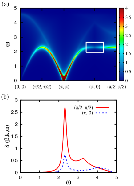
Figure 3: Modified dynamical structure factor $S(\beta,{\bf k},\omega)$ within the MFSB (eq. (3)). For $\beta^{*}={0.315}$ the sum rule is fulfilled (eq. (12)). (a) intensity curve along a path of the Brillouin zone. The white box shows the anomalous behavior at $(\pi,0)$ . (b) comparison between ${\bf k}=(\frac{\pi}{2},\frac{\pi}{2})$ (solid line) and ${\bf k}=(\pi,0)$ (dashed line).

4 Summary and concluding remarks

Motivated by the recent inelastic neutron scattering experiments performed in CFDT [8], the experimental realization of the square-lattice quantum antiferromagnet, we have investigated the anomaly found in the spectrum at $(\pi,0)$ using mean field Schwinger bosons. Based on the proposal that such anomaly could be due to the quantum mechanical destructive interference of the RVB component of the ground state [14], we have studied the spectrum by exploiting the ability of the MFSB to properly describe the magnetic excitations above the Néel and the averaged RVB components of the ground state. In particular, we have found that the triplet $D^{\dagger}_{\bf k}$ bond spin excitations, the natural excitations above the averaged RVB, have an anomalous spectral property at $(\pi,0)$ that can be associated to the above mentioned interference. Then, in order to improve the original dynamical structure factor $S({\bf k},\omega)$ [13] we have proposed a combined magnetic excitation $(1-\beta){S}{{}^{z}}_{\bf k}+\beta D^{\dagger}_{\bf k}$ that gives rise to a modified dynamical structure factor $S(\beta,{\bf k},\omega)$. Remarkably, once it is optimized to enforce the sum rule, the main features of the spectrum at low and high energies are reproduced quite well. Unfortunately the optimized $S(\beta^{*},{\bf k},\omega)$ does not recover the rotonic feature at $(\pi,0)$ but this is because the local constraint is not imposed exactly. If it is imposed carefully [29], as it has also been done in the fermionic spinon case [8], the rotonic features will be recovered. Regarding the possibility that free bosonic spinons can survive, or not, at $(\pi,0)$ is an issue that is beyond the scope of the present work. However, we think that the present results are calling for a more sophisticated calculation of the dynamical structure factor within the context of the Schwinger boson formalism, such as variational Monte Carlo [29, 30, 31] or 1/N correction [13, 27, 32, 33]. Work in the latter direction is in progress.

- [1] \NameAnderson P. W. \ReviewScience 235 (1987) 1196.
- [2] \NameManousakis E. \Review Rev. Mod. Phys. 63 (1991) 1.
- [3] \NameBaskaran G., Zou Z. and Anderson P. W. \ReviewSolid State Commun. 63 (1987) 973. \NameLiang S., Doucot B. and Anderson P. W. \ReviewPhys. Rev. Lett. 61 (1988) 365. \NameKotliar G. \ReviewPhys. Review B 37 (1988) 3664. \NameAffleck I. and Marston J. B. \ReviewPhys. Rev. B 37 (1988) 3774. \NameHsu T. C. \ReviewPhys. Rev. B 41 (1990) 11379. \NameHo C. M., Muthukumar V. N., Ogata M. Anderson P. W. \ReviewPhys. Rev. Lett. 86 (2001) 1626. \NameGhaemi P. and Senthil T. \ReviewPhys. Rev. B 73 (2006) 54415.
- [4] \NameFaddeev L. D., Takhtajan L. A. \ReviewPhys. Lett. A 85 (1981) 375.
- [5] \Name Nagler S. E., Tennant D. A., Cowley R. A., Perring T. G., Satija S. K. \ReviewPhys. Rev. B 44 (1991) 12361.
- [6] \NameTennant D. A., Perring T. G., Cowley R. A. and Nagler S. E. \ReviewPhys. Rev. Lett. 70 (1993) 4003.
- [7] \NameMourigal M., Enderle M., Klöpperpieper A., Caux J. S., Stunault A. and Rønnow H. M. \ReviewNat. Phys. 9 (2013) 435.
- [8] \NameDalla Piazza B., Mourigal M., Christensen N. B., Nilsen G. J., Tregenna-Piggott P., Perring T. G., Enderle M., McMorrow D. F., Ivanov D. A. and Rønnow H. M. \ReviewNat. Phys. 11 (2015) 62.
- [9] \NameColdea R,, Hayden S. M., Aeppli, Perring T. G., Frost C. D., Mason E., Cheong S.-W. and Z. Fisk \ReviewPhys. Rev. Lett. 86 (2001) 5377. \NamePeres N. M. R. and Araujo M. A. N. \ReviewPhys. Rev. B 65 (2002) 132404. \NameCapriotti L., Låuchli A. and Paramekanti A. \ReviewPhys. Rev. B 72 (2005) 214433. \NameHeadings N. S., Hayden S. M., Coldea R. and Perring T. G. \ReviewPhys. Rev. Lett. 105 (2010) 247001. \NameDean M. P. M., Springell R. S., Monney C., Zhou K. J., Pereiro J., Božović I., Dalla Piazza B., Rønnow H. M., Morenzoni E., van den Brink J., Schmitt T. and Hill J. P. \ReviewNat. Mat. 11 (2012) 850.
- [10] \NameZheng, W., Oitmaa, J. and Hamer, C. J. \ReviewPhys. Rev. B 71 (2005) 184440.
- [11] \NameSyljuåsen, O. F. and Rønnow, H. M. \ReviewJ. Phys. Condens. Matter 12, (2000) L405.
- [12] \NamePowalski M., Uhrig G. S. and Schmidt K. P. \ReviewPhys. Rev. Lett. 115 (2015) 207202.
- [13] \NameAuerbach A. and Arovas D. P. \ReviewPhys. Rev. Lett. 61 (1988) 617; \NameArovas D. P. and Auerbach A. \ReviewPhys. Rev. B 38 (1988) 316.
- [14] \NameChristensen, N. B., Rønnow H. M., McMorrow D. F., Harrison A., Perring T. G., Enderle M., Coldea R., Regnault L. P. and Aeppli G. \ReviewProc. Natl Acad. Sci. USA 104 (2007) 15264.
- [15] For frustrated AF it has been discussed in the literature the necessity of using a second singlet bond operator[16, 17, 18] but for the unfrustrated case it is enough the original formulation with only the singlet bond operator .
- [16] \NameCeccatto H. A., Gazza C. J. and Trumper A. E. \ReviewPhys. Rev. B 47 (1993) 12329.
- [17] \NameFlint R. and Coleman P. \ReviewPhys. Rev. B 79 (2009) 014424.
- [18] \NameMezio A., Sposetti C. N., Manuel L. O. and Trumper A. E. \ReviewEurophys. Lett. 94 (2011) 47001.
- [19] \NameChandra P., Coleman P. and Larkin A. I. \ReviewJ. Phys. Condens. Matter 2 (1990) 7933.
- [20] \NameZhong Q. F. and Sorella S. \ReviewEurophys. Lett. 21 (1993) 629.
- [21] \NameYoshioka D. \ReviewJ. Phys. Soc. Jpn. 58 (1989) 3733.
- [22] \NameSarker S, Jayaprakash C, Krishnamurthy H R and Ma M. \ReviewPhys. Rev. B40 (1989) 5028.
- [23] \NameMermin N D and Wagner H \ReviewPhys. Rev. Lett. 17 (1966) 1133.
- [24] \NameFradkin E. and Shenker S. H. \ReviewPhys. Rev. D 19 (1979) 3682.
- [25] \NameStarykh O. A. and Reiter G. \ReviewPhys. Rev. B 49 (1994) 4368.
- [26] \NameMezio A., Manuel L. O., Singh R. R. P. and Trumper A. E. \ReviewNew J. Phys. 14 (2012) 123033.
- [27] \NameRaykin M. and Auerbach A. \ReviewPhys. Rev. B 47 (1993) 5118.
- [28] \NameWang F. and Tao R. \ReviewPhys. Rev. B 61 (2000) 3508.
- [29] \NameChen Y. C. and Xiu K. \ReviewPhys. Lett. A 181 (1993) 373.
- [30] \NameMiyazaki T., Yoshioka D. and Ogata M. \ReviewPhys. Rev. B 51 (1995) 2966.
- [31] \Name Li T. Becca F., Hu W. and Sorella S. \ReviewPhys. Rev. B 86 (2012) 075111.
- [32] \NameTrumper A. E., Manuel L. O., Gazza C. J. and Ceccatto H. A. \ReviewPhys. Rev. Lett. 78, (1997) 2216.
- [33] \NameShindou R., Yunoki S., and Momoi T. \ReviewPhys. Rev. B 87, (2013) 054429.