Topological phase transitions on a triangular optical lattice with non-Abelian gauge fields

Abstract

We study the mean-field BCS-BEC evolution of a uniform Fermi gas on a single-band triangular lattice, and construct its ground-state phase diagrams, showing a wealth of topological quantum phase transitions between gapped and gapless superfluids that are induced by the interplay of an out-of-plane Zeeman field and a generic non-Abelian gauge field.

I Introduction

The intriguing possibility of superfluid (SF) phase transitions from topology in momentum $(\mathbf{k})$ space has long been of interest not only to the condensed-matter but also to the cold atom and molecular physics communities in the broad contexts of nodal superconductors ($d$-wave symmetry for high-$T_{c}$ materials), nodal SFs ($p$-wave symmetries for liquid ³He and single-component Fermi gases), and population-imbalanced SFs ($s$-wave symmetry for two-component Fermi gases) volovik07 . Analogous to the Lifshitz transition in metals lifshitz63 , these topological phase transitions are solely associated with the appearance or disappearance of $\mathbf{k}$-space regions with zero excitation energies, where the symmetry of the SF order parameter remains unchanged in sharp contrast to the Landau’s classification of ordinary phase transitions. Not only such changes naturally cause a dramatic rearrangement of particles in $\mathbf{k}$ space, and therefore, are readily seen in their $\mathbf{k}$-resolved distribution and/or spectral function, but they also leave non-analytic signatures in the thermodynamic properties of the system iskin06 .

To observe and study topological phase transitions, one requires to have a reliable knob over either the density of particles or both the strength and symmetry of the inter-particle interactions read00 . Since such controls are either very limited or not yet possible in condensed-matter systems, the cold-atom systems initially thought to offer an ideal platform for realizing these transitions, thanks in particular to their precise-tuning capabilities over a wide range of laser parameters. However, despite all the past and ongoing attempts with Fermi gases across $p$-wave Feshbach resonances gaebler07 ; inada08 ; fuchs08 ; maier10 , the short lifetimes of the resultant $p$-wave molecules have so far been the biggest drawback in this line of research, which the experimentalists yet to overcome.

On the other hand, given the recent progress in creating artificial gauge fields dalibard11 ; galitski13 , there is a growing consensus that one of the most promising ways to realize a topological phase transition is to incorporate $s$-wave Fermi gases with spin-orbit couplings (SOC) sato09 . For instance, depending on the inter-particle interaction, polarization, dimension, geometry, and symmetry and strength of SOC, it is possible to create a zoo of nodal SFs with point, line or surface nodes in $\mathbf{k}$ space in various numbers. Since several groups have already succeeded in creating such setups at high temperatures wang12 ; cheuk12 ; williams13 ; fu13 , there is arguably no doubt that these new systems will soon offer unforeseen possibilities once they are cooled below the required SF transition temperature. Stimulated by these experiments, there has been a fruitful activity on many aspects of spin-orbit coupled Fermi gases, but the majority of them are focused on continuum systems with a lack of interest in lattice ones zhai14 . For instance, even though topological SFs have recently been charecterized for a square lattice with non-Abelian gauge fields kubasiak10 ; iskin16 , and tunable honeycomb lattices (made of two triangular sublattices) are of both ongoing experimental and theoretical interest tarruell12 ; struck12 ; hauke12 ; jotzu14 ; kim13 , the triangular lattices themselves are almost entirely overlooked in this context.

Here, we study the BCS-BEC evolution of a spin-$1/2$ Fermi gas on a single-band triangular lattice, and construct its ground-state phase diagrams. Our primary objective is to establish that the interplay of an out-of-plane Zeeman field and a generic non-Abelian gauge field gives rise to a wealth of topological phase transitions between gapped and gapless SFs that are accessible in atomic optical lattices. The rest of the paper is organized as follows. After we introduce the model Hamiltonian in Sec. II, first we discuss the effects of a generic non-Abelian gauge field on the single-particle problem, and then briefly summarize the mean-field formalism that is used for tackling the many-body problem. In Sec. III, we thoroughly analyze the conditions under which the quasiparticle/quasihole excitation spectrum of the SF phase may vanish, and evaluate the corresponding changes in the underlying Chern number. These conditions are numerically solved in Sec. IV together with the self-consistency equations, where we construct the ground-state phase diagrams as a function of particle filling and SOC for a wide range of polarizations and interactions. The paper ends with a briery summary of our conclusions and an outlook given in Sec. V.

II Theoretical Model

In this paper, we consider a spin-$1/2$ Fermi gas on a triangular lattice, and study the effects of the following non-Abelian gauge field $\mathbf{A}=(\alpha\sigma_{y},-\beta\sigma_{x})$ on the ground state SF phases, where $\{\alpha,\beta\}\geq 0$ characterize the SOC, and $\sigma_{x}$ and $\sigma_{y}$ are the Pauli-spin matrices kubasiak10 ; iskin16 . We take the gauge field into account via the Peierls substitution, under which the tunneling of atoms from site $i$ to $j$ is described by the hopping Hamiltonian $H_{0}=-\sum_{\sigma\sigma^{\prime}ij}c_{\sigma^{\prime}j}^{\dagger}t_{ji}^{\sigma^{\prime}\sigma}c_{\sigma i}.$ Here, we only allow nearest-neighbor hoppings with $t_{ji}^{\sigma^{\prime}\sigma}=te^{-i\int_{\mathbf{r_{i}}}^{\mathbf{r_{j}}}\mathbf{A}\cdot d\mathbf{r}},$ where $t\geq 0$ is its amplitude, and $\mathbf{r_{i}}$ is the position of site $i$. The lattice spacing $a$ is set to unity in this paper. Using the Fourier series expansion of the annihilation operator $c_{\sigma i}=(1/\sqrt{M})\sum_{\mathbf{k}}e^{{\rm i}\mathbf{k}\cdot\mathbf{r_{i}}}c_{\sigma\mathbf{k}}$ and its Hermitian conjugate in momentum $\mathbf{k}=(k_{x},k_{y})$ space, where $M\to\infty$ is the number of lattice sites in the system, the hopping Hamiltonian can be written as $H_{0}=\sum_{\mathbf{k}}\psi_{\mathbf{k}}^{\dagger}(\epsilon_{\mathbf{k}}\sigma_{0}+\mathbf{S}_{\mathbf{k}}\cdot\vec{\sigma})\psi_{\mathbf{k}}.$ Here, the spinor $\psi_{\mathbf{k}}^{\dagger}=(c_{\uparrow\mathbf{k}}^{\dagger},c_{\downarrow\mathbf{k}}^{\dagger})$ denotes the creation operators, $\epsilon_{\mathbf{k}}$ is the energy dispersion, $\sigma_{0}$ is the identity matrix, $\mathbf{S}_{\mathbf{k}}=(S_{\mathbf{k}}^{x},S_{\mathbf{k}}^{y},0)$ is the SOC, and $\vec{\sigma}=(\sigma_{x},\sigma_{y},\sigma_{z})$ is a vector of spin matrices. For a triangular crystal lattice with primitive unit vectors $\mathbf{a_{1}}=(1,0)$ and $\mathbf{a_{2}}=(1/2,\sqrt{3}/2)$, we find

$$\epsilon_{\mathbf{k}} =-2t\cos\alpha\cos k_{x}-4t\cos\gamma\cos\frac{k_{x}}{2}\cos\frac{\sqrt{3}k_{y}}{2},$$ (1)

$$S_{\mathbf{k}}^{x} =-2\sqrt{3}t\beta\frac{\sin\gamma}{\gamma}\cos\frac{k_{x}}{2}\sin\frac{\sqrt{3}k_{y}}{2},$$ (2)

$$S_{\mathbf{k}}^{y} =2t\sin\alpha\sin k_{x}+2t\alpha\frac{\sin\gamma}{\gamma}\sin\frac{k_{x}}{2}\cos\frac{\sqrt{3}k_{y}}{2},$$ (3)

where $\gamma=\sqrt{\alpha^{2}+3\beta^{2}}/2$. Note that the reciprocal of a triangular lattice is a hexagonal lattice in $\mathbf{k}$ space with primitive unit vectors $\mathbf{b_{1}}=(2\pi,-2\pi/\sqrt{3})$ and $\mathbf{b_{2}}=(0,4\pi/\sqrt{3})$, and therefore, the first BZ is bounded by $|k_{y}|=2\pi/\sqrt{3}$ for $|k_{x}|\leq 2\pi/3$, $k_{y}=\pm(\sqrt{3}k_{x}-4\pi/\sqrt{3})$ for $2\pi/3\leq k_{x}\leq 4\pi/3$ and $k_{y}=\pm(\sqrt{3}k_{x}+4\pi/\sqrt{3})$ for $-4\pi/3\leq k_{x}\leq-2\pi/3$. In addition, since the area of the first BZ is $8\pi^{2}/\sqrt{3}$, we evaluate the sums $\sum_{\mathbf{k}}$ by converting them into integrals $[M\sqrt{3}/(8\pi^{2})]\int_{\textrm{BZ}}d^{2}\mathbf{k}$ in our numerics.

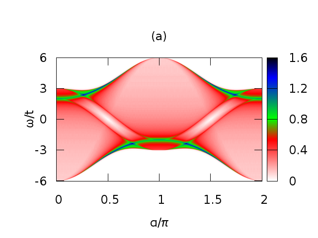
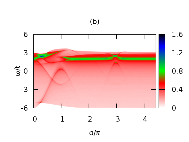
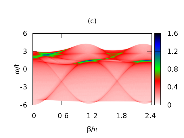
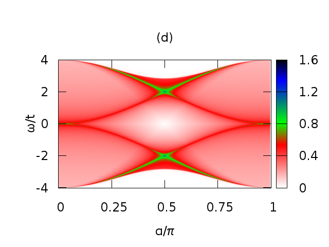
Figure 1: (Color online) The total DoS $tD(\omega)$ is shown as a function of energy $\omega/t$ and SOC $(\alpha,\beta)$ for (a) $\alpha=\beta$, (b) $\beta=\pi/4$, (c) $\alpha=\pi/4$, and (d) $\alpha=\beta$ (square lattice).

The total single-particle density-of-states (DoS) for the hopping Hamiltonian can be written as $D(\omega)=D_{+}(\omega)+D_{-}(\omega)$, where $D_{\pm}(\omega)=(1/M)\sum_{\mathbf{k}}\delta(\omega-\epsilon_{\mathbf{k}}\mp|S_{\mathbf{k}}|)$ with $\delta(x)$ the Dirac-delta function. In Fig. 1, we show colored maps of $tD(\omega)$ as a function of $\omega/t$ and $(\alpha,\beta)$, where $\pi\delta(x)\to\eta/(x^{2}+\eta^{2})$ is implemented in our numerics with a small broadening $\eta=0.01t$. First of all, after summing over $\mathbf{k}$, since the SOC can be gauged away from the single-particle problem in the limits of $\alpha\to 0$ or $\beta\to 0$, $D(\omega)$ approach to the no-SOC value in all figures, showing a sharp peak at $\omega=2t$. This is also the reason behind the somewhat featureless structure of Fig. 1(b) where $\beta$ is small. Furthermore, for symmetric SOCs with $\alpha=\beta$, it can analytically be shown that the DoS has $D(\omega,\alpha)=D(\omega,-\alpha),$ $D(\omega,\pi+\alpha)=D(\omega,\pi-\alpha)$ and $D(\omega,\alpha)=D(-\omega,\pi-\alpha)$ symmetries for any $\alpha$, leading to $D(\omega=0,\alpha=i\pi/2)=0$ for any integer $i$. These symmetries and the resultant gaps are clearly illustrated in our numerics shown in Fig. 1(a), and they play important roles in understanding the resultant ground-state SF phases as discussed below in Sec. IV. Thus, in sharp contrast to the continuum systems where the low-energy DoS increases with increasing SOC, we show that the DoS has a much richer dependence on energy and SOC on a triangular lattice. For completeness, typical DoS data are illustrated in Figs. 1(b) and 1(c) for asymmetric SOCs with $\alpha\neq\beta\neq 0$, showing no particular symmetry in general. In comparison to Fig. 1(a), we also show the analogous DoS dependence for a nearest-neighbor square lattice in Fig. 1(d), manifesting the particle-hole symmetry around $\omega=0$ for any $\alpha$.

Since our primary objective in this paper is to characterize distinct SF phases of $\uparrow$ and $\downarrow$ fermions in the presence of on-site attractive interactions in between, we introduce a complex parameter $\Delta_{i}=g\langle c_{\uparrow i}c_{\downarrow i}\rangle,$ which describes the local SF order within the BCS mean-field description, where $g\geq 0$ is the strength of the interaction, and $\langle\cdots\rangle$ is a thermal average. Finally, including a possible out-of-plane Zeeman field $h$, the total mean-field Hamiltonian can be compactly written as iskin16 $H=M|\Delta|^{2}/g+\sum_{\mathbf{k}}\xi_{\mathbf{k}}+(1/2)\sum_{\mathbf{k}}\Psi_{\mathbf{k}}^{\dagger}H_{\mathbf{k}}\Psi_{\mathbf{k}},$ where the operator $\Psi_{\mathbf{k}}^{\dagger}=(c_{\uparrow\mathbf{k}}^{\dagger},c_{\downarrow\mathbf{k}}^{\dagger},c_{\uparrow,-\mathbf{k}},c_{\downarrow,-\mathbf{k}})$ denotes the creation and annihilation operators collectively, the matrix

$$H_{\mathbf{k}}=\left(\begin{array}[]{cccc}\xi_{\mathbf{k}}-h&S_{\mathbf{k}}^{\perp}&0&\Delta\\ S_{\mathbf{k}}^{\perp*}&\xi_{\mathbf{k}}+h&-\Delta&0\\ 0&-\Delta^{*}&-\xi_{\mathbf{k}}+h&S_{\mathbf{k}}^{\perp*}\\ \Delta^{*}&0&S_{\mathbf{k}}^{\perp}&-\xi_{\mathbf{k}}-h\end{array}\right)$$ (8)

is the Hamiltonian density, $\xi_{\mathbf{k}}=\epsilon_{\mathbf{k}}-\mu$ with $\mu$ the chemical potential, $S_{\mathbf{k}}^{\perp}=S_{\mathbf{k}}^{x}-{\rm i}S_{\mathbf{k}}^{y}$ is the SOC, and the SF order parameter $\Delta=g\sum_{\mathbf{k}}\langle c_{\uparrow\mathbf{k}}c_{\downarrow,-\mathbf{k}}\rangle$ is uniform in $\mathbf{k}$ space. The eigenvalues $E_{\lambda\mathbf{k}}$ of the Hamiltonian matrix with $\lambda=\{1,2,3,4\}$ are simply given by $E_{\lambda\mathbf{k}}=s_{\lambda}\sqrt{\xi_{\mathbf{k}}^{2}+h^{2}+|\Delta|^{2}+|S_{\mathbf{k}}^{\perp}|^{2}+2p_{\lambda}A_{\mathbf{k}}},$ corresponding to the quasiparticle ($s_{1,3}=p_{3,4}=+1$) and quasihole ($p_{1,2}=s_{2,4}=-1$) excitation energies of the system, where $A_{\mathbf{k}}=\sqrt{(\xi_{\mathbf{k}}^{2}+|\Delta|^{2})h^{2}+|S_{\mathbf{k}}^{\perp}|^{2}\xi_{\mathbf{k}}^{2}}.$ In terms of $E_{\lambda\mathbf{k}}$, the self-consistency equations can be written as iskin16

$$-M\frac{|\Delta|}{g} =\frac{1}{4}\sum_{\lambda\mathbf{k}}\frac{\partial E_{\lambda\mathbf{k}}}{\partial|\Delta|}f(E_{\lambda\mathbf{k}}),$$ (9)

$$N_{\uparrow}+N_{\downarrow} =\frac{1}{4}\sum_{\lambda\mathbf{k}}\left[1-2\frac{\partial E_{\lambda\mathbf{k}}}{\partial\mu}f(E_{\lambda\mathbf{k}})\right],$$ (10)

$$N_{\downarrow}-N_{\uparrow} =\frac{1}{2}\sum_{\lambda\mathbf{k}}\frac{\partial E_{\lambda\mathbf{k}}}{\partial h}f(E_{\lambda\mathbf{k}}),$$ (11)

where $f(x)=1/[e^{x/(k_{B}T)}+1]$ is the Fermi function with $k_{B}$ the Boltzmann constant and $T$ the temperature. Here, the derivatives are $\partial E_{\lambda\mathbf{k}}/\partial|\Delta|=(1+p_{\lambda}h^{2}/A_{\mathbf{k}})|\Delta|/E_{\lambda\mathbf{k}}$ for the order parameter, $\partial E_{\lambda\mathbf{k}}/\partial\mu=-[1+p_{\lambda}(h^{2}+|S_{\mathbf{k}}^{\perp}|^{2})/A_{\mathbf{k}}]\xi_{\mathbf{k}}/E_{\lambda\mathbf{k}}$ for the chemical potential, and $\partial E_{\lambda\mathbf{k}}/\partial h=-[1+p_{\lambda}(\xi_{\mathbf{k}}^{2}+|\Delta|^{2})/A_{\mathbf{k}}]h/E_{\lambda\mathbf{k}}$ for the Zeeman field. While $\mu$ determines the total number $N=N_{\uparrow}+N_{\downarrow}$ of atoms where $N_{\sigma}=\sum_{i}n_{\sigma i}$ with the local fermion filling $0\leq n_{\sigma i}=\langle c_{\sigma i}^{\dagger}c_{\sigma i}\rangle\leq 1,$ $h\geq 0$ determines the polarization $P=(N_{\uparrow}-N_{\downarrow})/N\geq 0$ of the system which is assumed to be positive without loosing generality. Next, we analyze $E_{\lambda\mathbf{k}}$ for gapped/gapless solutions to distinguish SF phases by the $\mathbf{k}$-space topology of their excitations.

III Topological Superfluids

It is clear that $E_{1\mathbf{k}}$ and $E_{2\mathbf{k}}$ may become gapless in $\mathbf{k}$ space, i.e., $E_{1(2)\mathbf{k_{0}}}$ are precisely 0 at some special $\mathbf{k_{0}}$ points satisfying the condition $|S_{\mathbf{k_{0}}}^{\perp}|=0$ when $h=h_{\mathbf{k_{0}}}=\sqrt{(\epsilon_{\mathbf{k_{0}}}-\mu)^{2}+|\Delta|^{2}}.$ There are five sets of $\mathbf{k_{0}}$ points satisfying $|S_{\mathbf{k_{0}}}^{\perp}|=0$: in addition to the center $\mathbf{k_{1}}=(0,0)$ of the hexagon-shaped BZ, the two-point set $\mathbf{k_{2}}=(0,\pm 2\pi/\sqrt{3})$ corresponds to the midpoints of the top and bottom edges of the BZ adding in total to one full point, the four-point set $\mathbf{k_{3}}=(\pm\pi,\pm\pi/\sqrt{3})$ corresponds to the midpoints of the right and left edges of the BZ adding in total to two full points, the two-point set $\mathbf{k_{4}}=(k_{4}^{x},0)$ is such that $\cos\frac{k_{4}^{x}}{2}=-\frac{\alpha}{\sin\alpha}\frac{\sin\gamma}{2\gamma},$ and finally the four-point set $\mathbf{k_{5}}=(k_{5}^{x},\pm 2\pi/\sqrt{3})$ where $\cos\frac{k_{5}^{x}}{2}=\frac{\alpha}{\sin\alpha}\frac{\sin\gamma}{2\gamma}$ corresponds to two half-points on the top and two half-points on the bottom edges adding in total to two full points. Note that $k_{5}^{x}=k_{4}^{x}\pm 2\pi$ can only be satisfied in the first BZ for $\alpha=\beta$, in which case the combined set $\mathbf{k_{4}}=(\pm 4\pi/3,0)$ and $\mathbf{k_{5}}=(\pm 2\pi/3,\pm 2\pi/\sqrt{3})$ corresponds to the six corners of the BZ adding in total to two full points. Therefore, either the set $\mathbf{k_{4}}$ or $\mathbf{k_{5}}$ but not both is relevant when $\alpha\neq\beta$ as illustrated in Fig. 2. The corresponding energy dispersions at the location of zeros are $\epsilon_{\mathbf{k_{1}}}=-2t(\cos\alpha+2\cos\gamma)$ for the first set, $\epsilon_{\mathbf{k_{2}}}=-2t(\cos\alpha-2\cos\gamma)$ for the second set, $\epsilon_{\mathbf{k_{3}}}=2t\cos\alpha$ for the third set, and $\epsilon_{\mathbf{k_{4}}}=\epsilon_{\mathbf{k_{5}}}=2t\cos\alpha\left(1-\frac{\alpha^{2}}{\sin^{2}\alpha}\frac{\sin^{2}\gamma}{2\gamma^{2}}\right)+t\frac{\alpha}{\sin\alpha}\frac{\sin(2\gamma)}{\gamma}$ for the remaining sets.

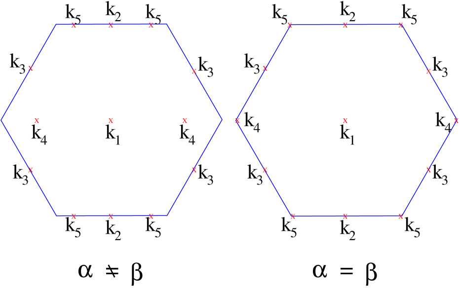
Figure 2: (Color online) The gapless $\mathbf{k}$-space points are illustrated within the first BZ. Note that either the set $\mathbf{k_{4}}$ or $\mathbf{k_{5}}$ but not both is relevant when $\alpha\neq\beta$ (see the text).

It is well-known that opening or closing of a gap in $\mathbf{k}$ space gives rise to a topological phase transition between SFs with distinct $\mathbf{k}$-space topologies. In our case, these transitions are further signalled by changes in the topological invariant of the system belissard95 , which by definition may only change due to a change in system’s underlying topology. For instance, it can be shown that the change in CN at $h=h_{\mathbf{k_{0}}}$ is simply given by a sum over the Berry indices at all touching points kubasiak10 ; iskin16 $\Delta{\rm CN}(h_{\mathbf{k_{0}}})=\sum_{\mathbf{k_{0}}}{\rm sign}(Y_{\mathbf{k_{0}}})$ where $Y_{\mathbf{k_{0}}}=\left[\frac{\partial S_{\mathbf{k}}^{x}}{\partial k_{x}}\frac{\partial S_{\mathbf{k}}^{y}}{\partial k_{y}}-\frac{\partial S_{\mathbf{k}}^{y}}{\partial k_{x}}\frac{\partial S_{\mathbf{k}}^{x}}{\partial k_{y}}\right]_{\mathbf{k_{0}}}.$ In particular, we find that $Y_{\mathbf{k_{1}}}=6t^{2}\alpha\beta\left(\frac{\sin\alpha}{\alpha}+\frac{\sin\gamma}{2\gamma}\right)\frac{\sin\gamma}{\gamma}$ is always positive and $\Delta{\rm CN}(h_{\mathbf{k_{1}}})=+1$, $Y_{\mathbf{k_{2}}}=-6t^{2}\alpha\beta\left(\frac{\sin\alpha}{\alpha}-\frac{\sin\gamma}{2\gamma}\right)\frac{\sin\gamma}{\gamma}$ is always negative and $\Delta{\rm CN}(h_{\mathbf{k_{2}}})=-1$, $Y_{\mathbf{k_{3}}}=-3t^{2}\alpha\beta\frac{\sin^{2}\gamma}{\gamma^{2}}$ is always negative and $\Delta{\rm CN}(h_{\mathbf{k_{3}}})=-2$, and $Y_{\mathbf{k_{4}}}=Y_{\mathbf{k_{5}}}=3t^{2}\alpha\beta\left(\frac{\sin^{2}\gamma}{\gamma^{2}}-\frac{\alpha^{2}}{\sin^{2}\alpha}\frac{\sin^{4}\gamma}{4\gamma^{4}}\right)$ is always positive and $\Delta{\rm CN}(h_{\mathbf{k_{4}}})=\Delta{\rm CN}(h_{\mathbf{k_{5}}})=+2$. Note that the total change in CN adds up to 0 for all parameters as a function of increasing $h$. This is because since the SF phase is topologically trivial in the $h\to 0$ limit, the normal phase must also be topologically trivial in the $h\gg t$ as well. In particular, when $\alpha=\beta$, these expressions reduce to $Y_{\mathbf{k_{1}}}=-3Y_{\mathbf{k_{2}}}=-3Y_{\mathbf{k_{3}}}=4Y_{\mathbf{k_{4}}}=4Y_{\mathbf{k_{5}}}=9t^{2}\sin^{2}\alpha,$ and the corresponding energy dispersions are given by $\epsilon_{\mathbf{k_{1}}}=-3\epsilon_{\mathbf{k_{2}}}=-3\epsilon_{\mathbf{k_{3}}}=-2\epsilon_{\mathbf{k_{4}}}=-2\epsilon_{\mathbf{k_{5}}}=-6t\cos\alpha$. Thus, since the combined set $\{\mathbf{k_{4}},\mathbf{k_{5}}\}$ corresponds to the six corners of the first BZ as illustrated in Fig. 2, and $h_{\mathbf{k_{2}}}=h_{\mathbf{k_{3}}}$ and $h_{\mathbf{k_{4}}}=h_{\mathbf{k_{5}}}$ are two-fold degenerate, we find $\Delta{\rm CN}(h_{\mathbf{k_{1}}})=+1$, $\Delta{\rm CN}(h_{\mathbf{k_{2,3}}})=-3$ and $\Delta{\rm CN}(h_{\mathbf{k_{4,5}}})=+2$. Based on this classification scheme, next we explore the phase diagrams of the system for SF phases with distinct $\mathbf{k}$-space topologies.

IV Self-Consistent Results

For simplicity, we restrict our numerical analysis to the ground state with symmetric SOCs, and solve the self-consistency Eqs. (9), (10) and (11) at $T=0$ as a function of total particle filling $F=(N_{\uparrow}+N_{\downarrow})/M$ and $\alpha=\beta$. We construct the ground-state phase diagrams for a number of polarization $P=(N_{\uparrow}-N_{\downarrow})/(N_{\uparrow}+N_{\downarrow})$ and $g$ values. Note that since $0\leq N_{\sigma}/M\leq 1$ within the single-band approximation, the maximum possible value of $F$ depends on $P$, i.e., $F_{\textrm{max}}=2/(1+|P|)$ and the majority (minority) component is a band insulator (normal) for $F\geq F_{\textrm{max}}$. In addition, since the phase diagrams are symmetric around $\pi$ with $\alpha\to 2\pi-\alpha$ symmetry, which is caused by the symmetry of the DoS as shown in Fig. 1(a), we present the resultant phase diagrams only for the interval $0\leq\alpha\leq\pi$.

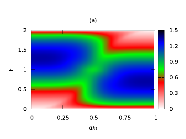
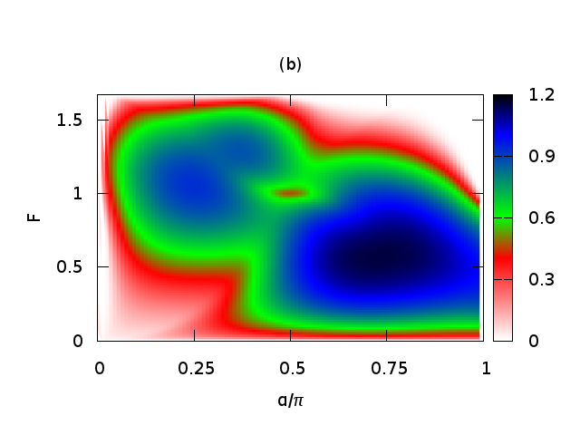
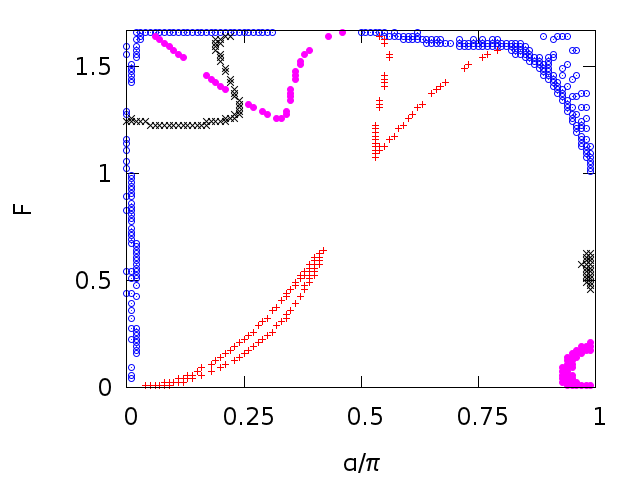
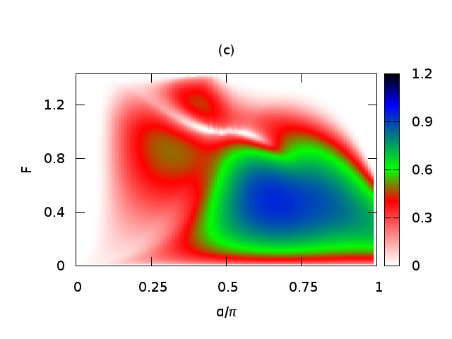
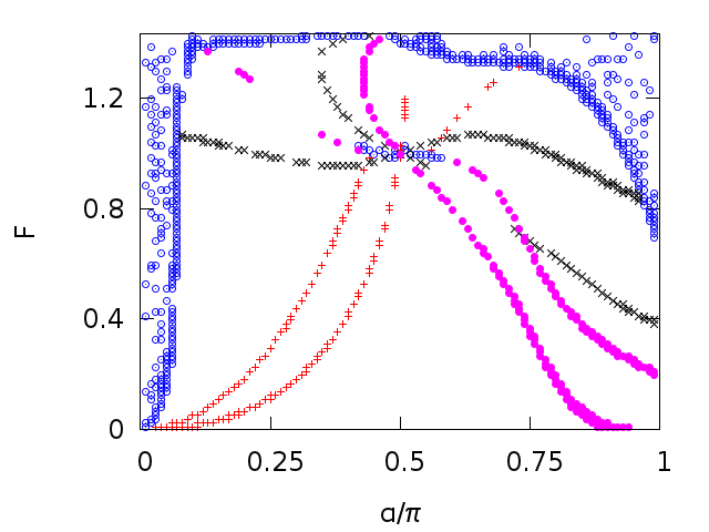
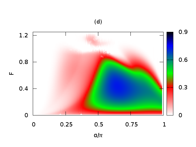
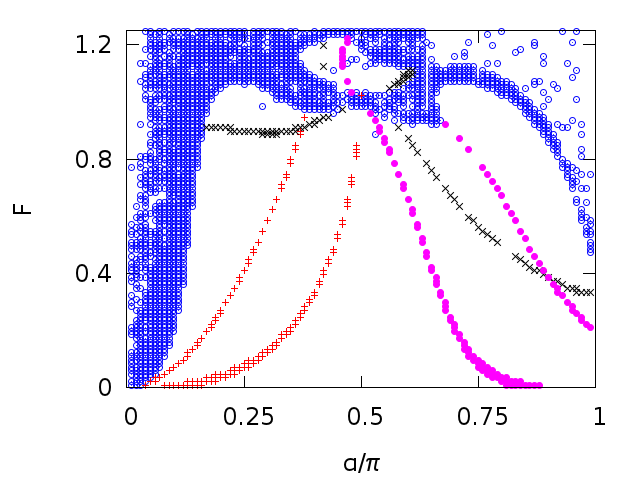
Figure 3: (Color online) The SF order parameter $|\Delta|/t$ (left) and the extracted boundaries for the topological quantum phase transitions (right) are shown as a function of total particle filling $F$ and SOC $\alpha=\beta$ for (a) $P=0$, (b) $0.2$, (c) $0.4$ and (d) $0.6$, where $g=4t$.

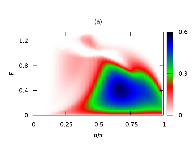
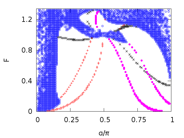
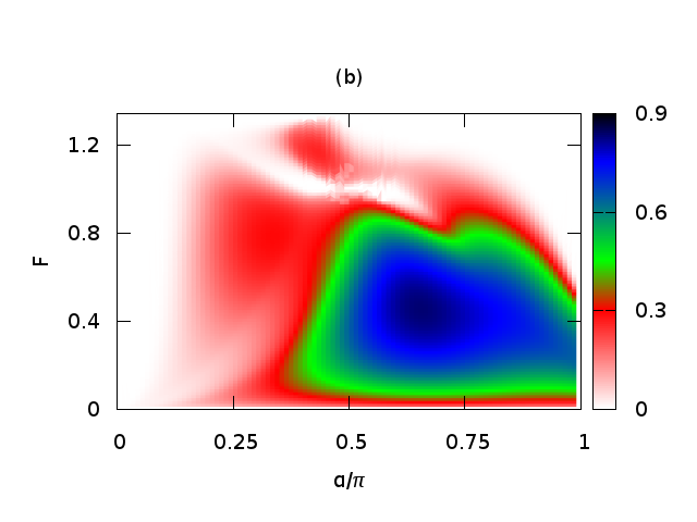
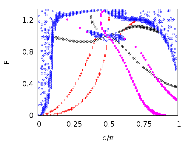
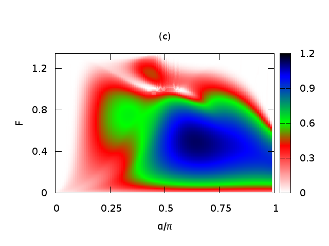
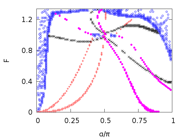
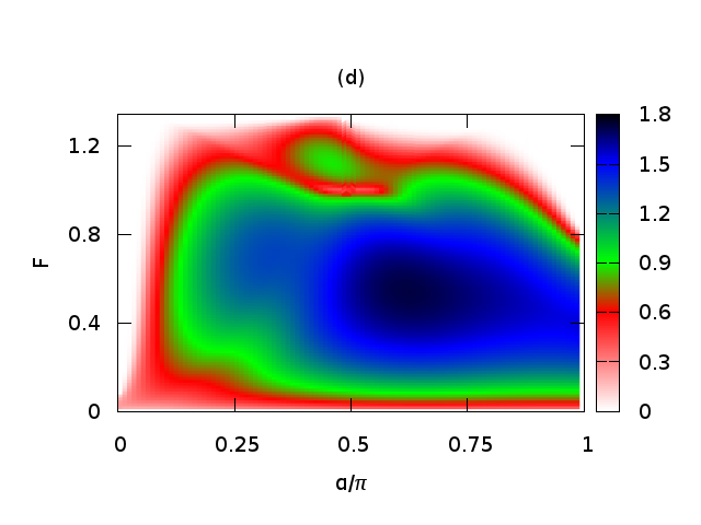
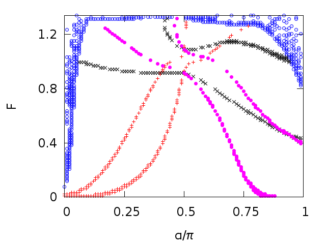
Figure 4: (Color online) The SF order parameter $|\Delta|/t$ (left) and the extracted boundaries for the topological quantum phase transitions (right) are shown as a function of total particle filling $F$ and SOC $\alpha=\beta$ for (a) $g=3t$, (b) $4t$, (c) $5t$ and (d) $7t$, where $P=0.5$.

For instance, in Fig. 3, we show colored maps of $|\Delta|/t$ and the corresponding boundaries for the topological quantum phase transitions when $g=4t$ and $P=\{0,0.2,0.4,0.6\}$. Here, the normal region is characterized by $|\Delta|\lesssim 10^{-3}t$. In the trivial case of zero polarization shown in Fig. 3(a), the entire phase diagram is a SF and even though some of the low-energy features are smeared out by finite $g$, $|\Delta|$ has precisely the symmetry of the DoS shown in Fig. 1(a), where $\omega=0$ corresponds to $\mu=0$, i.e., the half-filling $F=1$. As increasing $P$ progressively weakens $|\Delta|$ due to the Zeeman-induced pairing mismatch between $\uparrow$ and $\downarrow$ fermions, not only the normal region expands but also more footprints of the low-energy DoS become gradually salient in $|\Delta|$, including the gap at $\omega=0$ when $\alpha=\pi/2$. In particular, we find reentrant SF phase transitions that are interfered by the normal phase in the neighbourhood of this gap in Figs. 3(c) and 3(d). Furthermore, while the SF phase is trivially gapped in the entire phase diagram shown in Fig. 3(a), having a finite $P$ gives rise to the emergence of two phase-transition branches per each $\mathbf{k_{i}}$, satisfying the critical condition $h=h_{\mathbf{k_{i}}}$. These branches arise from the particle- and hole-pairing sectors, and all of them eventually meet at $F=1$ and $\alpha=\pi/2$ with increasing $P$. Since $\mu=0$ for all parameters as long as $F=1$, and $\epsilon_{\mathbf{k_{i}}}=0$ for all $\mathbf{k_{i}}$ points at $\alpha=\beta=\pi/2$, all of the transition boundaries become degenerate precisely when $h=|\Delta|$ is simultaneously satisfied. Therefore, the critical value of $P$ for such a crossing clearly increases with $g$, and it happens around $P_{c}\approx 0.2$ when $g=4t$ and $P_{c}\approx 0.4$ when $g=10t$.

Similarly, in Fig. 4, we show colored maps of $|\Delta|/t$ and the corresponding boundaries for the topological quantum phase transitions when $P=0.5$ and $g=\{3,4,5,7\}$. The intricate dependence of $|\Delta|$ on $F$ and $\alpha$, and the resultant reentrant SF phase transitions can again be traced back to the low-energy features of DoS, as they play the most important roles in the weakly-interacting limit where the reentrant behavior is most eminent for any $P$. Apart from the shrinkage of the normal region and gradual disappearance of the reentrant behavior due to enhanced pairing, one of the most notable findings in Fig. 4 is that not only the qualitative but also the quantitative structure of the phase diagrams are quite robust against increasing $g$. Thus, we conclude that topological phase transitions with $\Delta{\rm CN}=\{\pm 1,\pm 2,\pm 3\}$ are generally accessible on a triangular lattice. Having achieved our primary objective of constructing the ground-state phase diagrams, next we end this paper with a briery summary of our conclusions and an outlook.

V Conclusions

In summary, to describe the BCS-BEC evolution of a spin-$1/2$ Fermi gas that is loaded on a uniform triangular optical lattice, here we considered a single-band lattice Hamiltonian within the mean-field approximation for on-site pairing. In particular, we explored topological phase transitions between gapped and gapless SF phases that are induced by the interplay of an out-of-plane Zeeman field and a non-Abelian gauge field. These transitions are signalled by changes in the underlying Chern number, and we found that $\Delta{\rm CN}=\{\pm 1,\pm 2,\pm 3\}$ are generally accessible on a triangular lattice. By constructing a number of ground-state phase diagrams self-consistently for a wide range of parameter space, we also found reentrant SF phase transitions that are interfered by the normal phase, and traced their imprints to the DoS of the non-interacting problem. In sharp contrast to the continuum systems where the low-energy DoS increases with increasing SOC, we showed that the DoS has a much richer dependence on energy and SOC on a triangular lattice, leading in return to an intricate dependence of the SF order parameter on particle filling, SOC and inter-particle interaction. Since the low-energy DoS plays the most important role in the weakly-interacting limit, the reentrant behavior is most eminent there for any polarization, and it gradually diminishes as the interaction gets stronger.

Even though the topological phase transitions discussed in this paper occur in momentum space, and therefore, are most evident in the momentum distributions of atoms in time-of-flight measurements, it is well-established in the context of unconventional (e.g., $p$- or $d$-wave) nodal-SFs that such changes also leave non-analytic traces in the thermodynamic properties of the system including the compressibility, spin susceptibility, specific heat, etc. Thus, as an outlook, we believe it is fruitful to extend this line of research towards all sorts of directions, including finite center-of-mass pairings, finite temperatures, multi-band lattices, longer-ranged hoppings/interactions, Abelian gauge fields, confined systems, hexagonal lattices, higher-dimensional lattices, beyond mean-field effects, etc. Theoretical understanding of these extensions in greater depth will surely have dramatic impacts for not only to the cold-atom and condensed-matter communities but also to the others, where the interplay of SF pairing and SOC are contemporary concepts offering futuristic technological applications.

VI Acknowledgments

We gratefully acknowledge funding from TÜB$\dot{\mathrm{I}}$TAK Grant No. 1001-114F232.

References

- (1) For instance, see the review by G.E. Volovik, Quantum phase transitions from topology in momentum space, Lect. Notes Phys. 718, (2007).
- (2) For instance, see the review by I. M. Lifshitz and M. I. Kaganov, Some problems of the electron theory of metals II. Statistical mechanics and thermodynamics of electrons in metals, Sov. Phys. Usp. 5, 878 (1963).
- (3) M. Iskin and C. A. R. Sá de Melo, Nonzero orbital angular momentum pairing in superfluid Fermi gases, Phys. Rev. A 74, 013608 (2006).
- (4) N. Read and D. Green, Paired states of fermions in two dimensions with breaking of parity and time-reversal symmetries and the fractional quantum Hall effect, Phys. Rev. B 61, 10267 (2000).
- (5) J. P. Gaebler, J. T. Stewart, J. L. Bohn, and D. S. Jin, -Wave Feshbach Molecules, Phys. Rev. Lett. 98, 200403 (2007).
- (6) Y. Inada, M. Horikoshi, S. Nakajima, M. Kuwata-Gonokami, M. Ueda, and T. Mukaiyama, Collisional Properties of -Wave Feshbach Molecules, Phys. Rev. Lett. 101, 100401 (2008).
- (7) J. Fuchs, C. Ticknor, P. Dyke, G. Veeravalli, E. Kuhnle, W. Rowlands, P. Hannaford, and C. J. Vale, Binding energies of 6Li -wave Feshbach molecules, Phys. Rev. A 77, 053616 (2008).
- (8) R. A. W. Maier, C. Marzok, C. Zimmermann, and P. W. Courteille, Radio-frequency spectroscopy of 6Li p-wave molecules: Towards photoemission spectroscopy of a p-wave superfluid, Phys. Rev. A 81, 064701 (2010).
- (9) J. Dalibard, F. Gerbier, G. Juzelinas, and P. Öhberg, Colloquium: Artificial gauge potentials for neutral atoms, Rev. Mod. Phys. 83, 1523 (2011).
- (10) V. Galitski and I. B. Spielman, Spin-orbit coupling in quantum gases, Nature (London) 494, 49 (2013).
- (11) M. Sato, Y. Takahashi, and S. Fujimoto, Non-Abelian Topological Order in s-Wave Superfluids of Ultracold Fermionic Atoms, Phys. Rev. Lett. 103, 020401 (2009).
- (12) P. Wang, Z. Yu, Z. Fu, J. Miao, L. Huang, S. Chai, H. Zhai, and J. Zhang, Spin-orbit coupled degenerate Fermi gases, Phys. Rev. Lett. 109, 095301 (2012).
- (13) L. W. Cheuk, A. T. Sommer, Z. Hadzibabic, T. Yefsah, W. S. Bakr, and M. W. Zwierlein, Spin-Injection Spectroscopy of a Spin-Orbit Coupled Fermi Gas, Phys. Rev. Lett. 109, 095302 (2012).
- (14) R. A. Williams, M. C. Beeler, L. J. LeBlanc, K. Jiménez-García, and I. B. Spielman, Raman-induced interactions in a single-component Fermi gas near an s-wave Feshbach resonance, Phys. Rev. Lett. 111, 095301 (2013).
- (15) Z. Fu, L. Huang, Z. Meng, P. Wang, X.-J. Liu, H. Pu, H. Hu, and J. Zhang, Experimental realization of a two-dimensional synthetic spin-orbit coupling in ultracold Fermi gases, arXiv:1506.02861 (2015).
- (16) For instance, see the review by Hui Zhai, Degenerate quantum gases with spin orbit coupling: a review, Rep. Prog. Phys. 78 026001 (2015).
- (17) A. Kubasiak, P. Massignan, and M. Lewenstein, Topological superfluids on a lattice with non-Abelian gauge fields, Europhys. Lett. 92, 46004 (2010).
- (18) M. Iskin, Topological superfluids on a square optical lattice with non-Abelian gauge fields: Effects of next-nearest-neighbor hopping in the BCS-BEC evolution, to appear in Phys. Rev. A (2016).
- (19) L. Tarruell, D. Greif, T. Uehlinger, G. Jotzu, and T. Esslinger, Creating, moving and merging Dirac points with a Fermi gas in a tunable honeycomb lattice Nature 483, 302 (2012).
- (20) J. Struck, C. Ölschläger, M. Weinberg, P. Hauke, J. Simonet, A. Eckardt, M. Lewenstein, K. Sengstock, and P. Windpassinger, Tunable Gauge Potential for Neutral and Spinless Particles in Driven Optical Lattices, Phys. Rev. Lett. 108, 225304 (2012).
- (21) P. Hauke, O. Tieleman, A. Celi, C. Ölschläger, J. Simonet, J. Struck, M. Weinberg, P. Windpassinger, K. Sengstock, M. Lewenstein, and A. Eckardt, Non-Abelian Gauge Fields and Topological Insulators in Shaken Optical Lattices, Phys. Rev. Lett. 109, 145301 (2012).
- (22) G. Jotzu, M. Messer, R. Desbuquois, M. Lebrat, T. Uehlinger, D. Greif, and T. Esslinger, Experimental realization of the topological Haldane model with ultracold fermions, Nature (London) 515, 237 (2014).
- (23) D.-H. Kim, J. S. J. Lehikoinen, and P. Torma, Topological Transitions of Gapless Paired States in Mixed-Geometry Lattices, Phys. Rev. Lett. 110, 055301 (2013).
- (24) J. Bellissard, Change of the Chern number at band crossings, arXiv:cond-mat/9504030, unpublished (1995).