Interactions of the Infrared bubble N4 with the surroundings

Abstract

The physical mechanisms that induce the transformation of a certain mass of gas in new stars are far from being well understood. Infrared bubbles associated with H ii regions have been considered to be good samples for investigating triggered star formation. In this paper we report on the investigation of the dust properties of the infrared bubble N4 around the H ii region G11.898+0.747, analyzing its interaction with its surroundings and star formation histories therein, with the aim of determining the possibility of star formation triggered by the expansion of the bubble. Using Herschel PACS and SPIRE images with a wide wavelength coverage, we reveal the dust properties over the entire bubble. Meanwhile, we are able to identify six dust clumps surrounding the bubble, with a mean size of 0.50 pc, temperature of about 22 K, mean column density of 1.7 $\times 10^{22}$ cm^-2, mean volume density of about 4.4 $\times 10^{4}$ cm^-3, and a mean mass of 320 $M_{\odot}$. In addition, from PAH emission seen at 8 $\mu$m, free-free emission detected at 20 cm and a probability density function in special regions, we could identify clear signatures of the influence of the H ii region on the surroundings. There are hints of star formation, though further investigation is required to demonstrate that N4 is the triggering source.

1. Introduction

Massive stars (of OB spectral type with masses greater than $\sim 10M_{\odot}$) are thought to form in clusters within molecular cloud complexes. Intense radiative and mechanical outputs from massive stars strongly affect their parent molecular clouds in two opposite ways: by disrupting molecular clouds and by triggering star formation. In effect, on the one hand, the natal molecular clouds can be accelerated beyond their escape velocities by feedback from massive stars through expanding H ii regions, outflows, stellar winds, and supernova explosions, leading to the disruption of the clouds which can stop the eventual star-forming processes. On the other hand, this feedback is capable of sweeping up the surroundings and accumulating them into condensations gravitationally bound, inducing the formation of new generations of stars.

Over the past several decades, numerous studies have focused on star formation triggered in the environs of H ii regions (e.g., Deharveng et al., 2005, 2006; Zavagno et al., 2007; Deharveng et al., 2008, 2009; Ogura, 2010; Elmegreen, 2011; Kendrew et al., 2012; Dale et al., 2013; Samal et al., 2014; Liu et al., 2015; Dale et al., 2015). Two different mechanisms have been proposed as models of star formation triggered in the surroundings of H ii regions: the “collect and collapse” process (C & C, Elmegreen & Lada, 1977) and “radiation-driven implosion” (RDI, Bertoldi, 1989; Lefloch & Lazareff, 1994). In the C & C process, the ultraviolet radiation from ionizing sources produces an ionization front (IF), creating an expanding H ii region. The supersonic expansion of the H ii region drives the shock front (SF) in front of the IF. Finally, a shell of circumstellar gas can be collected between the IF and the SF. In due time, the shell may become denser and collapse to form stars. Several numerical simulations (e.g., Hosokawa & Inutsuka, 2005, 2006; Dale et al., 2007) have suggested that expanding H ii regions can trigger star formation through the C & C process only if ambient molecular material is massive enough. This process has been tentatively detected to be at work in several well-known H ii regions such as Sh 104 (Deharveng et al., 2003), RCW 79 (Zavagno et al., 2006), and RCW 120 (Deharveng et al., 2009). By contrast, in the RDI model, the IF drives the SF into molecular clouds surrounding the H ii region, stimulating the collapse of pre-existing subcritical clumps. Recent numerical simulations (e.g., Miao et al., 2006, 2009; Bisbas et al., 2011) have demonstrated that the RDI model can successfully interpret star formation in bright-rimmed clouds (BRCs). This prediction seems to have been confirmed by observations of BRCs (e.g., Reach et al., 2009; Liu et al., 2012) indicating that star formation concentrated along the central axis of the clouds might be the consequence of the RDI process.

Thompson et al. (2012) and Kendrew et al. (2012) speculated that around 14%-30% of the massive young stellar objects (MYSOs) in the Milky Way might have been induced by expanding bubbles/H ii regions on the basis of the association of a large sample of IR bubbles (Churchwell et al., 2006, 2007) with Red MSX MYSOs (Urquhart et al., 2008). However, the exact processes of triggered star formation are far from being understood. It is hoped that detailed studies of the physical interaction of bubbles/H ii regions together with their environs will lead to a better understanding of star formation associated with bubbles/H ii regions (Liu et al., 2015).

Far-infrared observations carried out by the Herschel Space Observatory enable us to get a better insight into the physical properties of the bubble / H ii region, with unprecedented resolutions and sensitivities in that spectral range. Thanks to the widespread wavelength coverage from 70 to 500 $\mu$m, the dust temperature and column density distributions of all of the entire bubbles/H ii regions can be readily revealed by fitting spectral energy distributions (SEDs) pixel by pixel. Additionally, Herschel observations can reveal star formation surrounding the system. The widespread coverage is adequate for better constraining the SED profiles of YSOs at earlier phases and more accurately estimating their physical parameters such as stellar mass and luminosity. Moreover, Herschel observations coupled with suitable molecular lines offering kinetic and dynamical information are very useful tools for understanding the interactions of the bubbles/H ii regions with their surroundings. The present paper presents a comprehensive study of the bubble N4 (Churchwell et al., 2006) using a combination of Herschel and molecular line observations.

The bubble N4 appears as an almost complete ring in the IR regime (see Figure 1), enclosing the H ii region G11.898+0.747 (Lockman, 1989). N4 is centered at $\alpha_{2000}=18^{\mathrm{h}}08^{\mathrm{m}}52\fs 80,\delta_{2000}=-18^{\circ}16\arcmin 22\farcs 8$, with a radius of $\sim 2\arcmin$, corresponding to $1.9\pm 0.5$ pc at a distance of $3.2\pm 0.9$ kpc (Churchwell et al., 2006). By analyzing the spatial distribution of candidate YSOs around N4, Watson et al. (2010) found no evidence for triggered star formation. However, they claimed that the presence of triggered star formation can not be ruled out due to the lack of a complete sample of the YSO population as well as maps of the molecular gas and ionized gas in the environs. In contrast, the expanding motion of N4 uncovered by the observations of $J=1-0$ of ¹²CO, ¹³CO, and C¹⁸O carried out by Li et al. (2013) suggests a signature of possible triggered star formation. Therefore, the issue of star formation in N4 merits a more comprehensive investigation.

The purpose of this study is to analyze interactions of the bubble N4 with its surroundings and star formation histories therein, and to explore the possibility of triggered star formation. This paper is organized as follows: the Herschel and molecular line observations together with archival IR and radio data are presented in Section 2, the results are described in Section 3, the discussion is arranged in Section 4, and finally, we give a summary in Section 5.

2. Observations and data reduction

2.1. Herschel Observations

The bubble N4 was observed as part of the Hi-GAL survey. In this survey, the Photodetector Array Camera $\&$ Spectrometer (PACS, Poglitsch et al., 2010) at 70 and 160 $\mu$m  and the Spectral and Photometric Imaging Receiver (SPIRE, Griffin et al., 2010) at 250, 350, and 500 $\mu$m  worked simultaneously in the parallel photometric mode. The observations were run in two orthogonal scanning directions at a scan speed of 60 arcsec s^-1. The measured angular resolutions of these bands are 10$\farcs$7, 13$\farcs$9, 23$\farcs$9, 31$\farcs$3, and 43$\farcs$.8 (Traficante et al., 2011), respectively, corresponding to $0.12\pm 0.05$ to $0.49\pm 0.21$ pc at the distance to N4. The detailed descriptions of the pre-processing of the data up to usable high-quality images can be found in Traficante et al. (2011).

To search for early stages of star formation in N4, we took 56 point sources from the Curvature Threshold Extractor package (CuTeX) catalog. They are encompassed within the 2.5 times radii of the bubble, of detection in the PACS 70 $\mu$m band. Details about the catalog and the photometric procedures considered in CuTeX can be found in Molinari et al. (2011).

2.2. Molecular Line Observations

Table 1Summary of KVN single-dish observations

Line	$\nu$	$\theta_{HPBW}$	$\eta$	$T_{sys}$	$T_{rms}$	$\delta V$
	GHz	arcsec		K	(K)	km s-1
H2O $6_{1,6}-5_{2,3}$	22.235077	120	0.46	80	0.05	0.21
CH3OH $7_{0,7}-6_{1,6}$	44.069476	60.5	0.48	170	0.07	0.11
HCO+ (1-0)	89.188526	31.5	0.38	250	0.08	0.05
o-H2CO $2_{1,2}-1_{1,1}$	140.83952	23.4	0.33	360	0.09	0.04

Single-dish observations of molecular lines were performed with the Korean VLBI Network (KVN) 21-m radio telescope at Yonsei site, Seoul on 2014 December 28. The front end of the single-dish telescope is equipped with the four receivers working at 22, 43, 86, and 129 GHz simultaneously. A digital filter bank (DFB) with a 64 MHz bandwidth split into 4096 channels was adopted, resulting in velocity resolutions of 0.21 km s^-1, 0.11 km s^-1, 0.05 km s^-1, and 0.04 km s^-1, respectively. The pointing and tracking accuracies were better than 3$\arcsec$ (Kim et al., 2011).

Since mapping observations are quite time-consuming, we only chose six dense clumps, located on the border of N4, to make single-point observations. To investigate the dynamical and kinetic properties (see Section 3.2 and 4.1) and star formation activity in the clumps, H₂O (22 GHz), CH₃OH (44 GHz), HCO⁺ (89 GHz), and o-H₂CO (141 GHz) were observed simultaneously. The data were calibrated to antenna temperature ($T_{a}^{*}$) using the chopper wheel method. A summary of observations is given in Table 1, including the half-power beam width ($\theta_{\mathrm{HPBW}}$), the beam efficiency ($\eta$), the typical systematic temperature ($T_{\mathrm{sys}}$), the rms noise level ($T_{\mathrm{rms}}$) and the velocity resolution ($\delta V$). The data were analyzed and visualized with the software GILDAS (Guilloteau & Lucas, 2000).

2.3. Archival data

To study the physical characteristics of the bubble and its associated YSO candidates, auxiliary data of images and point sources were complemented by the GLIMPSE (Benjamin et al., 2003), MIPSGAL (Carey et al., 2009) and WISE (Wright et al., 2010) surveys. The images of the Spitzer Infrared Array Camera (IRAC) at 3.6, 4.5, 5.8, and 8.0 $\mu$m, together with the Multiband Imaging Photometer for Spitzer (MIPS) at 24 $\mu$m were retrieved from the Spitzer Archive.. The angular resolutions of the images in the IRAC bands are $<2\arcsec$ and it is $\sim 6\arcsec$.0 in the MIPS 24 $\mu$m band. In addition, the WISE survey has mapped the entire sky in four infrared bands centered at 3.4, 4.6, 12, and 22 $\mu$m, with a resolution of 6$\farcs$1, 6$\farcs$4, 6$\farcs$5, and 12$\farcs$0, respectively (Wright et al., 2010). Point sources were obtained from the AllWISE Source and MIPSGAL Catalogs. Both catalogs contain the photometries of point sources cross matched with the Two Micron All Sky (2MASS, Skrutskie et al., 2006) survey. The 20 cm radio continuum image was used from the Multi-Array Galactic Plane Imaging Survey (MAGPIS, Helfand et al., 2006) archive was used to analyze the properties of the H ii region associated with N4, . Its angular resolution is less than 6$\farcs$0 and the sensitivity is better than 0.15 mJy beam^-1.

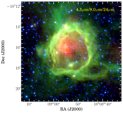
Figure 1.— Composite three-color image of N4. The IRAC 4.5 $\mu$m, 8.0 $\mu$m, and 24 $\mu$m are colored in blue, green, and red, respectively. The image is centered at $\alpha_{2000}=18^{\mathrm{h}}08^{\mathrm{m}}52\fs 80,\delta_{2000}=-18^{\circ}16\arcmin 22\farcs 8$.

3. Results

3.1. Dust Emission

3.1.1 Dust Temperature and Column Density Distributions

Herschel observations with the widespread wavelength coverage can reveal the dust properties of the entire bubble. To do this, a SED pixel-by-pixel fitting was performed to obtain the distributions of dust temperature ($T_{\mathrm{dust}}$) and H₂ column density ($N_{\mathrm{H_{2}}}$). Assuming optically thin dust emission, a graybody function for a single temperature can be expressed as follows:

$$I_{\nu}=\kappa_{\nu 0}(\nu/\nu_{0})^{\beta}\ B_{\nu}(T_{\mathrm{d}})\ \mu\ m_{\mathrm{H}}\ N(\mathrm{H}_{2}),$$ (1)

where $I_{\nu}$ is the surface brightness, $B_{\nu}(T_{\mathrm{d}})$ is the blackbody function for the dust temperature of $T_{\mathrm{d}}$, the mean molecular weight $\mu$ is assumed to be 2.8 (e.g., Kauffmann et al., 2008; Sadavoy et al., 2013); and $m_{\mathrm{H}}$ is the mass of a hydrogen atom. The dust opacity per unit mass of both dust and gas is defined as $\kappa_{\nu}=\kappa_{\nu 0}(\nu/\nu_{0})^{\beta}$, where $\kappa_{\nu 0}$ is assumed to be 0.1 cm${}^{2}~{}$g^-1 at 1 THz (Beckwith et al., 1990) under a gas-to-dust mass ratio of 100, and $\beta$ is fixed to 2, which is a statistical value found in a large sample of H ii regions (Anderson et al., 2012).

The Herschel data of the four bands at 160, 250, 350, and 500 $\mu$m  were used for the SED fitting. Since emission at 70 $\mu$m may trace hotter components such as very small grains (VSGs) and warmer material heated by protostars, it was not considered in the SED fitting for a single temperature. The four images were convolved to the same resolution 43$\farcs$8, and rebinned to the same pixel size 11$\farcs$5. To minimize the contribution from the line of sight, we subtracted the backgrounds for each image using a reference area away from the bubble. The corresponding backgrounds were estimated to be 634 MJy sr^-1 for 160 $\mu$m, 387 MJy sr^-1 for 250 $\mu$m, 205 MJy sr^-1 for 350 $\mu$m  and 79 MJy sr^-1 for 500 $\mu$m. By treating $T_{\mathrm{dust}}$ and $N_{\mathrm{H_{2}}}$ as free parameters, the SED fitting was performed using the IDL program MPFITFUN (Markwardt, 2009). In principle, the 870 $\mu$m image should have been considered in the SED fitting. Although the 870 $\mu$m data constrain the dust temperature, as they are sensitive to colder components than Herschel data, they miss the bulk of extended emission, which is the major interest in our current work. Thus, the image at 870 $\mu$m has been excluded in the SED fitting.

The resulting $T_{\mathrm{dust}}$ and $N_{\mathrm{H_{2}}}$ maps are shown in Figure 2, where the black contours stand for the emission at 24 $\mu$mand the purple contour delineates a level of $N_{\mathrm{H_{2}}}=9\times 10^{21}$ cm^-2, sculpting a shell structure. Emission traced by 24 $\mu$m mainly comes from hot dust which can reach very high temperatures after absorbing high-energy photons (e.g., Deharveng et al., 2010, references therein). The hot dust distribution shown in Figure 2(a) indicates a dust heating from the interior to the edge of N4 (also see Figure 1), therefore, possible temperature gradients along this direction would be expected. However, the dust distributions in the interior and on the edge of N4 appear to be smooth. Given the resolution of 6$\arcsec$ at 24 $\mu$m, the smoothness could be interpreted as the temperature gradients on small scales not resolved by the angular resolution of 43$\farcs$8 of the dust temperature map. Additionally, we note that there is a cold region of $\sim 22$ K within the bubble, which may be not real due to the low flux found there (Anderson et al., 2012).

On the large scale, the temperature distribution nearly matches with 24 $\mu$m emission (see Figure 2(a)). That is, the temperatures of cold dust in the bubble direction are hotter than those away the bubble, suggesting that the H ii region enclosed by N4 has been heating its surroundings. On the small scale, there are three regions that are especially warmer than other places in the $T_{\mathrm{dust}}$ map. The first region, located near the bubble center, it can be attributed to the heating of the central ionizing stars (see Section 3.4). The second warm region, with which some YSO candidates are associated (see Section 3.3), is to the north of N4. Hence, this warm region could be a result of the heating from embedded protostars therein. However, the third warm region in the northern border of N4 has no bright 24 $\mu$m counterpart or potential associated YSO candidate. Figure 2(b) shows that the column density of this region is lower than that of its neighbors. This difference suggests that this warm region may be heated premarily by the ionizing photons leaking from the H ii region.

For the H₂ column density distribution in Figure 2(b), a shell morphology is inscribed as seen in IR bands. In the shell, there is an anti-correlation between $N_{\mathrm{H_{2}}}$ and $T_{\mathrm{dust}}$. This may be attributed to a lower penetration of the external heating from the H ii region into dense regions. If the shell is bounded by a level of $9\times 10^{21}$ cm^-2 as shown in Figure 2(b), which covers a region of $\sim 1.5$ radius of the bubble, the mean $N_{\mathrm{H_{2}}}$ column density and total mass of the shell can be estimated to be $1.1\times 10^{22}$ cm^-2 and $5.2\times 10^{3}$ $M_{\odot}$, respectively. The total mass of the neutral material of the entire bubble is estimated to be $\sim~{}5.5\times 10^{3}$ $M_{\odot}$.

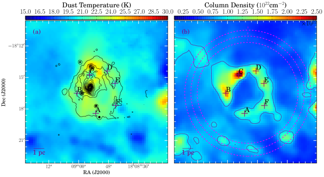
Figure 2.— Maps of the dust temperature (a) and the $\mathrm{H}_{2}$ column density (b) of N4. The two maps were all built on the SED fitting pixel by pixel, centered at $\alpha_{2000}=18^{\mathrm{h}}08^{\mathrm{m}}52\fs 80,\delta_{2000}=-18^{\circ}16\arcmin 22\farcs 8$. The crosses symbolize six dense clumps extracted from the $\mathrm{H}_{2}$ column density map. The purple contour shows a level of $9\times 10^{21}$ cm^-2, which covers a region of $\sim 1.5$ radius region of the bubble. Column density PDFs within the three magenta dashed circles are taken into account (see Section 4.2).

.

3.1.2 Dense Clumps

Six dense clumps were identified within the shell structure in the $\mathrm{H}_{2}$ column density image. These sources were decomposed visually from the image by ellipses bounded by the level of $9\times 10^{21}$ cm^-2 enclosing the majority of fluxes. The six clumps have different physical sizes and peak column densities ($N_{\mathrm{H_{2},peak}}$). Their average temperatures ($<T_{dust}>$) were obtained from the dust temperature image. We estimated the total mass (gas+dust) and the volume density for each clump.

Table 2Characteristics of six dust clumps

Name	R.A.	Decl.	$r_{major}$	$r_{minor}$	$r_{eff}\tablenotemark{a}$	$<T_{dust}>$	$N_{\mathrm{H_{2},peak}}$	$n_{\mathrm{H_{2}}}$	$M_{(gas+dust)}$
	(hh:mm:ss.ss)	(dd:mm:ss.s)	(arcsec)	(arcsec)	(pc)	(K)	(1022 cm-2)	(104cm-3)	(102 $M_{\odot}$)
A	18:08:53.14	-18:18:25.5	24.3	44.6	0.4 $\pm$ 0.1	22.3 $\pm$ 0.2	1.0 $\pm$ 0.1	4.0 $\pm$ 1.4	0.8 $\pm$ 0.5
B	18:09:00.66	-18:16:30.0	36.7	51.9	0.6 $\pm$ 0.2	22.1 $\pm$ 0.5	1.9 $\pm$ 0.3	5.0 $\pm$ 2.1	3.5 $\pm$ 2.5
C	18:08:55.59	-18:14:44.5	34.9	49.9	0.6 $\pm$ 0.2	23.1 $\pm$ 0.9	2.8 $\pm$ 0.5	7.8 $\pm$ 3.6	4.5 $\pm$ 3.4
D	18:08:48.57	-18:14:23.1	34.1	40.8	0.5 $\pm$ 0.1	22.3 $\pm$ 0.7	1.6 $\pm$ 0.2	5.2 $\pm$ 2.1	1.9 $\pm$ 1.3
E	18:08:45.39	-18:15:34.6	35.8	41.0	0.5 $\pm$ 0.2	21.7 $\pm$ 0.7	1.5 $\pm$ 0.1	4.7 $\pm$ 1.8	1.9 $\pm$ 1.3
F	18:08:45.18	-18:17:40.7	37.4	35.2	0.5 $\pm$ 0.1	23.6 $\pm$ 0.7	1.3 $\pm$ 0.1	4.4 $\pm$ 1.6	1.4 $\pm$ 0.9

Table 2 gives a summary of the aforementioned parameters, where the main source of error is the uncertainty of the distance to the bubble. The average size, dust temperature, column density, number density, and mass of the six clumps are $\sim 0.5$ pc, $\sim 22$ K, $\sim 1.7\times 10^{22}$ cm^-2, $\sim 4.4\times 10^{4}$ cm^-3, and $\sim 3.2\times 10^{2}$ $M_{\odot}$, respectively. The average density $>10^{4}$ cm^-3 is consistent with the detections of dense molecular lines within these clumps (see Section 3.2).

3.2. Molecular Line Emission

Table 3Parameters of molecular lines of the six dust clumps

	HCO+			o-H2CO
Name	$V_{LSR}$	$FWHM$	$T_{mb}$	$\int T_{mb}\ \mathrm{d}V$	$V_{LSR}$	$FWHM$	$T_{mb}$	$\int T_{mb}\ \mathrm{d}V$
	(km s-1)	(km s-1)	(K)	(K km s-1)	(km s-1)	(km s-1)	(K)	(K km s-1)
A	23.61 $\pm$ 0.06	2.62 $\pm$ 0.11	1.30 $\pm$ 0.12	3.62 $\pm$ 0.16	23.53 $\pm$ 0.25	2.30 $\pm$ 0.52	0.40 $\pm$ 0.11	0.99 $\pm$ 0.19
B	23.58 $\pm$ 0.06	2.03 $\pm$ 0.08	1.84 $\pm$ 0.12	4.01 $\pm$ 0.15	23.88 $\pm$ 0.08	1.91 $\pm$ 0.19	0.97 $\pm$ 0.11	1.98 $\pm$ 0.17
C-I	23.56 $\pm$ 0.21	2.54 $\pm$ 0.21	0.99 $\pm$ 0.11	3.84 $\pm$ 0.31	24.51 $\pm$ 0.38	4.32 $\pm$ 0.70	0.53 $\pm$ 0.12	2.42 $\pm$ 0.41
C-II	26.68 $\pm$ 0.06	1.79 $\pm$ 0.21	2.91 $\pm$ 0.11	4.74 $\pm$ 0.26	26.87 $\pm$ 0.04	1.16 $\pm$ 0.11	1.78 $\pm$ 0.12	2.19 $\pm$ 0.29
D	25.00 $\pm$ 0.06	3.06 $\pm$ 0.10	1.47 $\pm$ 0.11	4.77 $\pm$ 0.17	25.11 $\pm$ 0.12	2.00 $\pm$ 0.35	0.67 $\pm$ 0.11	1.43 $\pm$ 0.19
E	25.28 $\pm$ 0.06	2.46 $\pm$ 0.06	2.33 $\pm$ 0.11	6.12 $\pm$ 0.17	25.47 $\pm$ 0.09	2.23 $\pm$ 0.28	0.96 $\pm$ 0.12	2.26 $\pm$ 0.21
F	24.86 $\pm$ 0.09	4.02 $\pm$ 0.24	0.85 $\pm$ 0.12	3.64 $\pm$ 0.23	25.36 $\pm$ 0.20	2.91 $\pm$ 0.51	0.49 $\pm$ 0.11	1.53 $\pm$ 0.22

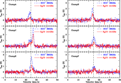
Figure 3.— HCO⁺ (1-0) and o-H₂CO $2_{1,2}-1_{1,1}$ spectra of the six clumps. The black dashed lines indicate a systematic velocity of 24.7 km s^-1 for the bubble. The systematic velocity is determined from the average spectra of the HCO⁺ and H₂CO lines of the six clumps, which is coincident with the results of ¹²CO, ¹³CO, and C¹⁸O (1-0) observations (Li et al., 2013). $T_{\mathrm{mb}}$ represents the main-beam temperature. The name of each clump is noted in the top left of each panel.

Figure 3 presents HCO⁺ (1-0) and o-H₂CO $2_{1,2}-1_{1,1}$ spectra of the six clumps. Since the molecules H₂O and CH₃OH were not detected, their spectra are not be displayed. Emission of HCO⁺ (1-0) and o-H₂CO $2_{1,2}-1_{1,1}$ is strong enough to be detected in all clumps. Their detections indicate high densities for the six clumps, since the critical densities of both lines are $4.5\times 10^{4}$ cm^-3, and $1.3\times 10^{5}$ cm^-3 for a kinetic temperature of 20 K (Shirley, 2015). Using the software GILDAS, we retrieved the observed parameters from the spectra of the six clumps, including the peak velocity ($V_{LSR}$), line width (FWHM) and the main-beam temperature ($T_{mb}$), and the velocity-integrated intensity ($\int T_{mb}\ \mathrm{d}V$) of the different spectra (see Table 3).

It is interesting to analyze the centroid velocity variances of the six clumps. The spectra of HCO⁺ and o-H₂CO obviously show the velocities blueshifted to a systematic velocity of 24.7 km s^-1in the southeastern (SE) part of the bubble (i.e., Clumps A and B) and the redshifted velocities in the northwestern (NW) part (i.e., Clumps D and E). The two remaining clumps show no evident velocity shifts. Observations of J=1-0 of ¹²CO, ¹³CO, and C¹⁸O also have already revealed the same velocity difference between the SE and the NW (see Figure 3 of Li et al., 2013). Due to the lack of blueshifted profiles in the front of the bubble and redshifted ones in the back cap of the bubble in the CO observations, Li et al. (2013) suggested that the bubble N4 may be expanding along the SE-NW direction with an inclination relative to the sky plane. This scenario is compatible with Beaumont & Williams (2010) interpretations of molecular gas studies around a number of IR bubbles, where they conclude that the SFs driven by massive stars tend to create rings. Therefore, the shell of dust and gas in the bubble N4 is presumably assembled by the expanding H ii region.

Assuming that the observed o-H₂CO line is optically thin and in local thermodynamic equilibrium (LTE), we estimate the column density of this molecular species toward each dense clump presented in Section 3.1.2 using (Goldsmith & Langer, 1999):

$$N=\frac{8\pi k\nu^{2}}{hc^{3}A_{ul}}\frac{Q_{rot}}{g_{u}}~{}{\rm exp}(\frac{E_{u}}{T_{rot}})\int{T_{mb}~{}{\rm dv}},$$ (2)

where $A_{ul}=5.4\times 10^{-5}$ s^-1, $E_{u}=21.9$ K, and $g_{u}=15$. Assuming that the dust and the gas are coupled at the same temperature, in LTE conditions we can approximate $T_{dust}=T_{kin}=T_{rot}$. Thus, for $T_{rot}$ we used the $T_{dust}$ value obtained for each clump (see Section 3.1.2). Given a temperature of $\sim 22$ K averaged over the six clumps, the o-H₂CO partition function $Q_{rot}$ was estimated to be $\sim 50$ by the extrapolation to the relation between $Q_{rot}$ and $T_{rot}$ from the CDMS Catalog. The obtained column density values for each clump are presented in Table 4, which also includes the o-H₂CO abundances ($X=$ N(o-H₂CO)/N(H₂)). The abundances were estimated using the H₂ column densities presented in Section 3.1.2. We note that o-H₂CO emission is generally optically thick, therefore, the assumption of optically thin emission of o-H₂CO results in underestimated column density and abundance.

The obtained o-H₂CO column densities and abundances are quite similar to those obtained toward other photo-dominated regions (PDRs), such as the Horsehead PDR (Guzmán et al., 2011), and the Orion Bar (van der Wiel et al., 2009, 2010). Considering that the dust grains are cold ($T_{dust}\sim 22$ K) in the dense clumps around the N4 bubble and given the abundances presented in Table 4, we suggest that in this region the formaldehyde may be formed mainly in the gas phase with a probable contribution of photo-desorption of the grain mantles as was found in the Horsehead PDR (Guzmán et al., 2011).

Observations of other o-H₂CO and p-H₂CO lines toward this region would be very useful to give an important observational probe of the gas phase and grain surface chemistry toward PDRs.

Table 4o-H₂CO LTE column densities and abundances.

Clump	N(o-H2CO)	$X$
	($\times 10^{12}$ cm-2)	(10-10)
A	6.26	6.2
B	12.66	6.6
C	28.20	9.9
D	9.05	5.6
E	14.61	9.7
F	9.13	7.0

3.3. YSOs Associated with N4

To understand more about star formation histories associated with the bubble, candidate YSOs associated with N4 have been initially identified using the online SED fitting tool of Robitaille et al. (2006, 2007) and then further demonstrated and classified with color-color diagrams. The SED fitting tool invokes a grid of 20,000 two-dimensional Monte Carlo radiation transfer models (e.g., Whitney et al., 2004). With 10 viewing angles for each model, there are actually 200,000 YSO SED models. This tool works as a linear regression method to fit these models to the multi-wavelength photometry measurements of a given source. The goodness/badness of each fit could be quantified by a specified value of the best $\chi^{2}$ ($\chi^{2}_{best}$), whereby YSO candidates could be robustly distinguished from reddened photospheres of main-sequence and giant stars since YSOs require a thermal emission component to reproduce the shapes of their mid-IR excesses. In addition, this method can make use of any available data to constrain the shape of SED profiles as well as possible (see Appendix A). However, we have to acknowledge that the disk and stellar parameters inferred from the SED models can be very uncertain (Offner et al., 2012, and T.P. Robitaille 2015, private communication). Therefore, if these uncertain parameters are used to classify the identified YSO candidates with the scheme of YSO classification of Robitaille et al. (2006), the classification results must be unreliable. To avoid this uncertainty, the color selection schemes of Gutermuth et al. (2009) and Koenig et al. (2012) have been adopted to group the YSO candidates identified by the SED fitting into three “Classes”: Class I, Class II, and Transition Disk (TD) YSOs. Class I objects are deeply embedded protostars with a dominant infalling envelope, Class II objects are surrounded by a substantial accreting disk (Lada, 1987), and TD objects are more evolved protostars where the inner parts of the disks have been cleared by photoevaporation of the central stars or by planet-forming processes (Gutermuth et al., 2009; Yuan et al., 2014; Paron et al., 2015). We believe that using the infrared color schemes is a better way to categorize the YSO candidates because the infrared color schemes are a powerful proxy for measuring the excess emission (e.g., Allen et al., 2004; Gutermuth et al., 2008, 2009; Koenig et al., 2012). Apart from this, the candidate YSOs, which have been singled out by the SED fitting, can be further confirmed by such color schemes.

Sixty potential YSOs within 5$\arcmin$ from the bubble center have been identified and classified. Of these, there are 8 Class I, 12 Class II, and 40 TD objects. The classification results are listed in Table 5 and the detailed processes can be found in the Appendix A. We note that the resulting 60 YSO candidates are incomplete but robust (see the Appendix A). Despite this incompleteness, the resulting population with robust identifications is enough for simply learning about the distributions of the YSOs associated with N4.

Figure 4 shows the spatial distribution of the 60 YSO candidates. One can see that the majority ($\sim 82\%$) of YSOs are spatially correlated with the PDRs as traced by 8 $\mu$m emission (see Section 3.4), which indicates the good spatial association of these potential YSOs with the bubble N4 and the strong impacts that the enclosed H ii region is having on the surrounding star formation. In addition, there is an overdensity of the number of YSO candidates residing on the verge of the bubble. This is also demonstrated by the statistics of all candidates as a function of the normalized bubble radius (see Figure 5). The statistics suggest that a large number ($\sim 40\%$) of YSO candidates is located within $1.0-1.5$ times the radius of the bubble. Such spatial distribution of YSOs in N4 agrees well with the statistical results based on the study of the association of a large sample of YSOs with IR bubbles (Kendrew et al., 2012; Thompson et al., 2012).

Table 5Parameters of YSO candidates

No.	Name	RA	Decl.	$N$	$\chi^{2}_{\mathrm{best}}$	Class
Y1	J180831.89-181639.1	272.133	-18.278	7	13.4	II
Y2	J180832.49-181616.6	272.135	-18.271	7	35.7	TD
Y3	J180834.88-181751.0	272.145	-18.298	7	18.3	TD
Y4	J180835.68-181814.8	272.149	-18.304	7	11.0	TD
Y5	J180839.36-181813.8	272.164	-18.304	7	20.9	TD
Y6	J180839.71-181841.5	272.165	-18.312	7	47.7	TD
Y7	J180840.11-181902.3	272.167	-18.317	7	21.6	TD
Y8	J180841.62-181600.0	272.173	-18.267	7	12.9	TD
Y9	J180842.08-181457.5	272.175	-18.249	7	8.2	TD
Y10	J180842.19-181329.1	272.176	-18.225	7	34.6	TD
Y11	J180842.69-181930.1	272.178	-18.325	7	34.0	TD
Y12	J180843.58-181441.8	272.182	-18.245	7	38.3	TD
Y13	J180844.11-181456.4	272.184	-18.249	7	30.4	TD
Y14	J180844.15-181401.9	272.184	-18.234	7	43.4	TD
Y15	J180844.97-181457.3	272.187	-18.249	7	40.2	TD
Y16	J180845.97-181612.4	272.192	-18.270	8	32.2	II
Y17	J180846.14-181844.0	272.192	-18.312	7	32.0	TD
Y18	J180847.47-181416.2	272.198	-18.238	7	22.3	TD
Y19	J180847.65-181450.0	272.199	-18.247	7	32.9	TD
Y20	J180847.67-181441.7	272.199	-18.245	7	12.6	TD
Y21	J180848.33-181357.2	272.201	-18.233	7	33.9	TD
Y22	J180849.08-181441.8	272.205	-18.245	4	0.2	I
Y23	J180849.78-181340.5	272.207	-18.228	7	6.5	TD
Y24	J180850.19-181816.2	272.209	-18.305	7	27.3	II
Y25	J180850.83-181836.6	272.212	-18.310	7	14.0	II
Y26	J180851.55-181831.9	272.215	-18.309	7	7.6	TD
Y27	J180852.42-181744.2	272.218	-18.296	7	22.5	II
Y28	J180852.59-181356.6	272.219	-18.232	7	7.4	II
Y29	J180852.97-181336.2	272.221	-18.227	7	43.8	TD
Y30	J180853.04-181742.2	272.221	-18.295	8	5.5	I
Y31	J180853.35-181130.9	272.222	-18.192	7	41.9	TD
Y32	J180853.65-181208.4	272.224	-18.202	7	29.8	TD
Y33	J180853.94-181422.4	272.225	-18.240	5	0.3	I
Y34	J180854.47-181406.5	272.227	-18.235	4	0.1	I
Y35	J180854.69-181230.5	272.228	-18.208	7	39.4	TD
Y36	J180854.87-181409.5	272.229	-18.236	4	0.1	I
Y37	J180855.80-181136.3	272.233	-18.193	7	16.7	TD
Y38	J180856.26-181505.7	272.234	-18.252	7	26.5	II
Y39	J180856.64-181420.4	272.236	-18.239	7	12.4	II
Y40	J180857.00-181354.7	272.238	-18.232	4	0.1	II
Y41	J180857.48-181853.3	272.240	-18.315	7	25.0	TD
Y42	J180858.07-181506.0	272.242	-18.252	7	12.8	TD
Y43	J180858.12-181807.2	272.242	-18.302	7	26.4	TD
Y44	J180858.75-181806.5	272.245	-18.302	7	22.4	TD
Y45	J180858.77-181629.7	272.245	-18.275	11	25.1	I
Y46	J180859.32-181316.1	272.247	-18.221	7	9.8	II
Y47	J180859.44-181332.8	272.248	-18.226	7	0.9	I
Y48	J180859.47-181855.8	272.248	-18.316	7	14.1	TD
Y49	J180900.26-181347.5	272.251	-18.230	7	11.3	TD
Y50	J180900.28-181921.8	272.251	-18.323	7	31.4	TD
Y51	J180900.48-181903.2	272.252	-18.318	7	28.2	TD
Y52	J180902.92-181316.2	272.262	-18.221	7	41.9	TD
Y53	J180904.56-181638.3	272.269	-18.277	7	6.6	TD
Y54	J180904.95-181806.2	272.271	-18.302	7	23.3	TD
Y55	J180905.60-181621.4	272.273	-18.273	8	2.1	II
Y56	J180906.19-181639.1	272.276	-18.278	7	0.9	TD
Y57	J180906.60-181847.9	272.278	-18.313	7	19.7	TD
Y58	J180908.60-181706.1	272.286	-18.285	7	39.2	TD
Y59	MG011.8545+00.7327	272.216	-18.313	10	8.7	I
Y60	MG011.9455+00.7481	272.248	-18.226	9	6.6	II

3.4. Properties of the Ionized Region

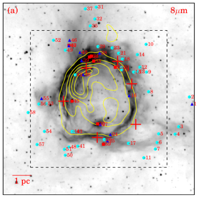
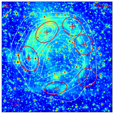
Figure 4.— (a) Image at 8 $\mu$m (grayscale) overlaid with free-free continuum emission at 20 cm (contours). The yellow contours start from $5\sigma$ (i.e., $1\sigma=0.15$ mJy Beam^-1) with a step of $8\sigma$. Class I, Class II, and transition disk YSO candidates are symbolized by square, triangle, and circle symbols, respectively. The dashed rectangle is a selected region for a close-up view of 4.5 $\mu$m emission. (b) Image at 4.5 $\mu$m (colorscale) overlaid with dust emission at 250 $\mu$m (contours). The white contours start from 18 Jy Beam^-1 with a step of 5.5 Jy Beam^-1. The ellipses depict the dust clumps extracted in Section 3.1.2, and the cross symbols represent their peak positions. A scale bar of 1 pc is shown on the bottom left.

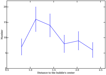
Figure 5.— Plot of the number counts of the 60 YSO candidates as a function of angular distance from the center of the bubble N4. The distance is normalized by the bubble radius. Error bars are determined via Poisson statistics.

Figure 4 (a) presents the 8 $\mu$m image overlaid with radiation at 20 cm. The 8 $\mu$m emission predominantly comes from two prominent polycyclic aromatic hydrocarbons (PAHs) at 7.7 $\mu$m and 8.6 $\mu$m. They are good tracers of PDRs delineating the IF created by massive stars. The 20 cm radiation represents free-free continuum emission from ionized gas. As shown in Figure 4 (a), most of the ionized gas is surrounded by the ring of PDRs, showing the strong effects of the H ii region on its surroundings. Additionally, the ring of PDRs is also spatially well correlated with the 250 $\mu$m emission (see Figure 4 (b)), which is sensible to cold dust in thermal equilibrium. As such, the cold dust wrapping ionized gas suggests a positive association of the bubble N4 with the H ii region, enhancing their intensive mutual interaction.

Several properties of the H ii region can be derived from 20 cm free-free continuum emission. Churchwell et al. (1978); Wink et al. (1983); Quireza et al. (2006) demonstrated the existence of a relationship between the H ii region electron temperature, $T_{e}$, and the Galactocentric distance, $R_{\mathrm{Gal}}$. A detailed analysis of a sample of 76 H ii regions with the highest quality data suggested that the electron temperature along the Galactic disk decreases approximately as a function of $R_{\mathrm{Gal}}$ (Quireza et al., 2006):

$$T_{e}=(5780\pm 350)+(287\pm 46)\ R_{\mathrm{Gal}}.$$ (3)

With an estimated Galactocentric distance of 5.5 kpc to N4, it yields an electron temperature of $7400\pm 600$ K. If the H ii region reaches the equilibrium at this temperature, the electron density, $n_{\mathrm{e}}$, the mass of ionized gas, $M_{\mathrm{ion}}$, and the Lyman photons per second, $N_{\mathrm{Lym}}$, from the exciting star(s), can be estimated following Kurtz et al. (1994):

$$n_{\mathrm{e}}=2.878\times 10^{4}\ [(\frac{\theta}{\mathrm{arcsec}})^{-3}\ (\frac{D}{\mathrm{kpc}})^{-1}\ (\frac{\nu}{\mathrm{GHz}})^{0.1}\ (\frac{T_{\mathrm{e}}}{\mathrm{K}})^{0.35}\ (\frac{S_{\nu}}{\mathrm{Jy}})]^{0.5}\ \mathrm{cm}^{-3},$$ (4)

$$M_{\mathrm{ion}}=\frac{4}{3}\ \pi\ r^{3}_{\mathrm{H{\,\sc{\mathrm{ii}}}}}\ n_{e}\ \ m_{\mathrm{\mathrm{p}}},$$ (5)

$$N_{\mathrm{Ly}}=7.588\times 10^{48}\ (\frac{T_{\mathrm{e}}}{\mathrm{K}})^{-0.5}\ (\frac{\nu}{\mathrm{GHz}})^{0.1}\ (\frac{S_{\nu}}{\mathrm{Jy}})\ (\frac{D}{\mathrm{kpc}})^{2}\ \mathrm{ph}\ \mathrm{s}^{-1},$$ (6)

where $S_{\nu}$ is the integrated flux density at the special frequency $\nu$ over the angular size $\theta$; $r_{\mathrm{H{\,\sc{\mathrm{ii}}}}}$ is the radius of the H ii region, and $m_{\mathrm{p}}$ is the proton mass. If the $\theta$ and $r_{\mathrm{H{\,\sc{\mathrm{ii}}}}}$ are considered to be approximately equal to those of the bubble, a total of $32.8\pm 0.01$ Jy at 20 cm measured by integrating over the 5 $\sigma$ contour (see Figure 4) yields an estimated $n_{\mathrm{e}}$, $M_{\mathrm{ion}}$, and $N_{\mathrm{Lym}}$ of $75\pm 15$ cm^-2, $50\pm 38$ $M_{\odot}$, and $(1.5\pm 1.1)\times 10^{48}$ $\mathrm{ph}\ \mathrm{s}^{-1}$, respectively. The errors of these parameters result mainly from the uncertainty in the distance of N4. According to Martins et al. (2005), the estimated $N_{\mathrm{Lym}}$ (Log($N_{\mathrm{Lym}}$) $\simeq 48.18$) indicates that a main O8.5V-O9V star was responsible for the ionization of N4. These are lower limits given that any ionizing photons absorbed by dust or moving away from the bubble were not accounted for.

The central exciting stars of N4 may be located near the very bright 24 $\mu$m emission inside the bubble. Based on the statistical analysis for the seven well-defined bubbles including N4, Deharveng et al. (2010) argued that the hot dust grains seen at 24 $\mu$m inside the ionized region can be heated by absorption of the Lyman continuum photons which are more numerous near exciting stars. This indicates that the ionizing stars of N4 may reside near the very bright 24 $\mu$m emission inside the bubble (see Figures 1 and 2(a)). This explanation can be further supported by the positive association of intense free-free continuum radiation from ionized gas with the bright 24 $\mu$m emission (see Figures 2(a) and 4(a)). Observations of spectroscopy of ionizing stars (Martins et al., 2010) are expected to reveal their natures.

4. Discussion

4.1. Star Formation in Clumps

The good agreement of the PDRs with cold dust emission and the associated YSO candidates therein are good indicators of the strong impact of the H ii region on its surroundings and on star formation processes. In what follows, we investigate the six identified dust clumps in a context of star formation within them.

In the case of the Aquila Rift complex, a column density threshold of $N_{\mathrm{H_{2}}}>7\times 10^{21}$ cm^-2 was estimated for the formation of prestellar cores (André et al., 2011). For the six clumps in N4, the mean column density of $1.4\times 10^{22}$ cm^-2 suggests that they may be capable of forming stars. A mass-size relationship is generally adopted to predict whether the clumps will form low-mass stars or high-mass stars (Kauffmann & Pillai, 2010). Based on the statistical analysis of nearby clouds without high-mass star formation (i.e., Pipe Nebula, Taurus, Perseus, and Ophiuchus) and known samples with high-mass star formation such as those of Beuther et al. (2002); Mueller et al. (2002); Hill et al. (2005), and Motte et al. (2007), a limiting mass-size relation of $m(r)\geq 870$ $M_{\odot}$ $(r/\mathrm{pc})^{1.33}$ was found to be an approximate threshold for high-mass star formation (Kauffmann & Pillai, 2010). Figure 6 shows the mass versus size relation for the six clumps in N4. Given uncertainties of the two parameters, the two clumps (Clumps B and C) are above the threshold, indicating that they may be forming massive stars, whereas the other four clumps below the threshold may be inclined to form low-mass stars. Indeed, several YSO candidates are close to all clumps but Clump F and six of these (Y22, Y33, Y34, Y36, Y45 and Y59, see Figure 4) are classified as Class I YSOs, however, there is no YSO candidate located at the peak positions of the six clumps. These facts suggest that the interiors of six clumps may be in the process of forming stars but without active ongoing star-forming activities.

No clear evidence for ongoing star formation has also been demonstrated in the observations of the four molecular lines toward the peak positions of the six clumps. The 22 GHz H₂O and 44 GHz Class I CH₃OH masers are known to occur in low- and/or high-mass star formation regions (e.g., Forster & Caswell, 1999; Kurtz et al., 2004). These two types of masers are generally thought to be associated with molecular outflows (e.g., Codella et al., 2004; Kurtz et al., 2004). Optically thick lines of HCO⁺ and H₂CO are widely used to search for asymmetric line profiles indicative of infall or outflow motions (e.g., Wu et al., 2007; Chen et al., 2010, and references therein). Therefore, these four molecular lines are an important signpost of ongoing star formation. In the bubble N4, it turns out that no detection of the 22 GHz H₂O and 44 GHz Class I CH₃OH masers has been obtained toward the peak positions of all clumps, and the asymmetric red profiles (i.e., a double peak spectral profile with red peak higher than blue peak) have been detected only in Clump C by the HCO⁺ and H₂CO lines (see Figure 3).

As a result, no scenario of ongoing star formation is confirmed in the center of any of the six clumps except for Clump C. On the one hand, this result may be a consequence of the poor angular resolution of the present observations (23-120$\arcsec$, corresponding to 0.26-1.35 pc). On the other hand, it can result from the incompleteness of the current sample of YSO candidates. Therefore, we have correlated the six clumps with the YSOs in the RMS survey database (Lumsden et al., 2013), the sources in the Methanol Multi-Beam survey (Green et al., 2010), and the compact H ii region catalog in the CORNISH survey (Purcell et al., 2013). It turns that there is only one source found in the RMS survey, which corresponds to the YSO candidate Y45 (see Figure 4). In addition, extended green objects (EGOs) identified based on their extended 4.5 $\mu$m emission are thought to be massive YSO outflow candidates (Cyganowski et al., 2008). Figure 4(b) shows Spitzer 4.5 $\mu$m emission overlaid with cold dust radiation at 250 $\mu$m. One can see that six clumps except for Clumps C and D peak at dark 4.5 $\mu$m emission, and no brighter extended 4.5 $\mu$m structures with respect to their backgrounds are detected for Clumps C and D, indicating that there may be either no active ongoing star formation or deeply embedded protostars at the centers of these clumps.

Due to the aforementioned lack of the H₂O, Class I CH₃OH maser detections, and other signs of ongoing star formation, it is difficult to confirm that the asymmetric red profiles are produced by outflow motions. The fact that Clump C is located close to the strong ionization zone implies that it is fully exposed to intense feedback from the main O8.5V-O9V star such as the compression of the ionized region and stellar winds, forming the different two different velocity components and leading to the asymmetric line profiles. Alternatively, this type of line profile may originate from the clump rotation. Hence, it is worthwhile to determine the mechanism responsible for the asymmetric line profile in Clump C using a map observation with higher angular resolution.

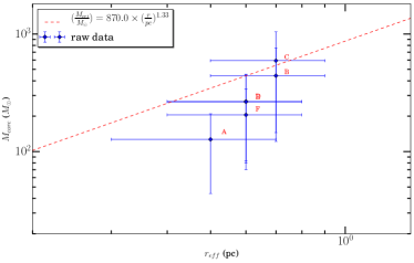
Figure 6.— Mass-size relationship of the six clumps. The dashed line represents an empirical relation of $m(r)=870$ $M_{\odot}$ $(r/\mathrm{pc})^{1.33}$, which is expected to be as a threshold for forming high-mass stars (Kauffmann & Pillai, 2010).

4.2. Feedback From Massive Stars

Massive stars are expected to affect their surroundings. Inside the bubble, the hot dust traced by 24 $\mu$m emission has been presumably heated by absorption of Lyman continuum photons whose free-free radiation is detected through radio continuum emission at 20 cm. At the edge of the bubble, the shell of cold dust emission is associated with the PDR that delimits the H ii region, indicating the bright illumination of the far UV photons created by massive stars. In the northeast of the bubble, brighter PAH emission is seen extending beyond the IF. This can be attributed to far UV photons leaking from the H ii region due to small-scale inhomogeneities in the IF and in the surrounding medium (Zavagno et al., 2007). Likewise, the southwestern filament with bright PAH emission can also be attributed to leaking radiation. All of the above observed facts demonstrate the strong influence of the expanding H ii region on the surroundings. Therefore, the YSO candidates associated with them must suffer the physical action of the H ii region. Moreover, 8 $\mu$memission shows concave-convex characteristics, indicating that the IF is locally distorted. The outline of the cold dust emission, and likewise that of the IF, shows that this type of distortion occurs in the adjacent clouds. In this case such distortion could be attributed to compressions of the expanding IF. Such compression can be characterized by the probability density function (PDF) of the column density.

In turbulent simulations (Tremblin et al., 2012a, b), it is argued that when the ionized gas pressure overweighs the ram pressure of the turbulence, the ionization compression could produce PDF forms with two lognormal distributions:

$$p(\eta)=\frac{p_{0}}{\sqrt{2\pi\sigma_{0}^{2}}}\exp\left(\frac{-(\eta-\mu_{0})^{2}}{2\sigma_{0}^{2}}\right)+\frac{p_{1}}{\sqrt{2\pi\sigma_{1}^{2}}}\exp\left(\frac{-(\eta-\mu_{1})^{2}}{2\sigma_{1}^{2}}\right),$$ (7)

where $\eta=\mathrm{ln}(N/\bar{N})$, $p_{i}$, $\mu_{i}$ and $\sigma_{i}$ are the integral, mean, and dispersion of each component, respectively. $\bar{N}$ represents the mean column density over a large region. The first lognormal form at low densities is generally thought to be a result of isothermal supersonic turbulence (Vazquez-Semadeni, 1994; Vázquez-Semadeni et al., 2008; Federrath et al., 2008; Federrath et al., 2010). The second lognormal distribution in the PDF at high densities is believed to be caused by the compression from the ionized gas pressure (Tremblin et al., 2012a, b, 2014). Currently, this sort of PDF form has been observed in several massive star-forming regions, and interpreted as ionization compressions (e.g., Schneider et al., 2012; Tremblin et al., 2014).

Therefore, the exploration of the PDF form in the bubble N4 can help to improve our understanding of the influences of the H ii region on the surroundings. The column density PDF is investigated over three regions (i.e., Circles 1, 2 and 3, see Figure 2) covering the ionized gas and the major surroundings. The three regions are concentric with an equal separation of 0.01 degree. Figure 7 displays the column density PDFs toward the three regions well fitted by the sum of two lognormal distributions. The mean column density $\bar{N}=8.0\times 10^{21}$ cm^-2 is averaged over the region of Circle 3. The fitting parameters can be found in Table 6. As shown in Figure 7, all the column density PDFs of the three regions show the second lognormal forms. Given the association of the H ii region with the bubble N4, these forms might be caused by compression of ionized gas. We note that the regions smaller than the Circle 1 do not fit two lognormal distributions well. This may be due to the fact that in this region there are not enough sample points. Furthermore, we observe that the integral of the second lognormal component ($p_{1}$) decreases as the radius of the target region increases. As suggested by Tremblin et al. (2014), this trend could be due to the fact that the larger the region is, the less important the amplitude of the compressed lognormal becomes since more unperturbed gas is added to the distribution, indicative of less significance of compression of the ionized gas in larger regions.

Table 6Parameters of the PDF fitting

Region	$p_{0}$	$\mu_{0}$	$\sigma_{0}$	$p_{1}$	$\mu_{1}$	$\sigma_{1}$
1	0.035	-0.091	0.200	0.006	0.430	0.238
2	0.035	-0.078	0.181	0.005	0.383	0.271
3	0.040	-0.081	0.200	0.003	0.488	0.221

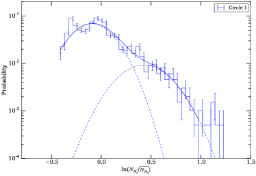
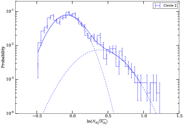
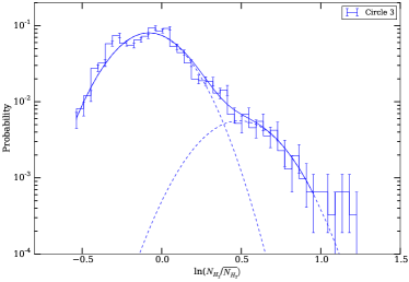
Figure 7.— Column density PDFs over the target regions (see Figure 2). $\overline{N_{\mathrm{H_{2}}}}$ represents mean the density. The best lognormal PDF fit (solid curve) is done by the sum of two lognormal distributions (dashed curves, see Eq. 7). Error bars are determined via Poisson statistics.

4.3. Collect and Collapse Process

The association of collected molecular gas with PDR regions and the compression from ionized gas confirm the strong influence of the H ii region on the adjacent medium. In the context of the C & C process, such an impact may stimulate the formation of a new generation of stars. To test the occurrence of this process, the dynamical time of the H ii region can be compared with the fragmentation time of the surrounding molecular clouds (Deharveng et al., 2003, 2005; Zavagno et al., 2006, 2007, 2010).

According to the well-known expansion law (Spitzer, 1978; Dyson & Williams, 1980), if an H ii region evolves in an homogeneous molecular cloud, the dynamical age ($t_{\mathrm{dyn}}$) of the H ii region can be expressed as follows:

$$R_{\mathrm{St}} = (3N_{\mathrm{Ly}}/4\pi n_{\mathrm{H},0}^{2}\alpha_{\mathrm{B}})^{1/3},$$

$$t_{\mathrm{dyn}} = \frac{4}{7}\ \frac{R_{\mathrm{St}}}{C_{\mathrm{H{\,\sc{\mathrm{ii}}}}}}\ [(\frac{R_{\mathrm{IF}}}{R_{\mathrm{St}}})^{7/4}-1],$$ (8)

where $R_{\mathrm{St}}$ is the radius of the Str$\mathrm{\ddot{o}}$mgren sphere, $n_{0}$ is the initial particle density of ambient neutral gas, $\alpha_{B}$ = $2.6\times 10^{-13}(10^{4}\mathrm{K}/T)^{0.7}$ cm³ s^-1 (Kwan, 1997) is the the coefficient of the radiative recombination, $C_{\mathrm{H{\,\sc{\mathrm{ii}}}}}$ is the isothermal sound speed of ionized gas assumed to be 10 km s^-1, and $R_{\mathrm{IF}}$ is the radius of the IF. If we assume that $R_{\mathrm{IF}}$ is approximately equal to the radius of N4, the total mass of $\sim 555$ $M_{\odot}$ of the neutral and ionized gas can yield an initial number density of $n_{\mathrm{H},0}=\sim 1.2\times 10^{4}$ cm^-3. Given the estimated $N_{\mathrm{Ly}}$ (see Section 3.4), $t_{\mathrm{dyn}}$ of N4 is therefore $\sim 1.0$ Myr. This timescale, however, is uncertain since the actual evolution of the H ii regions is not in a strictly uniform medium. Bearing this in mind, the estimated dynamical age should be considered with this caveat.

On the other hand, following Whitworth et al. (1994), gravitational fragmentation of the shell of collected material can be expected when

$$t_{\mathrm{frag}}=1.56\ a_{.2}{}^{7/11}N_{49}{}^{-1/11}n_{3}{}^{-5/11},$$ (9)

where $a_{.2}$ is the sound speed ($a_{s}$) inside the shell in units of 0.2 km s^-1, $N_{49}$ is the ionizing photon flux ($N_{Ly}$) in units of $10^{49}$ ph s^-1, and $n_{3}$ is the initial gas atomic number density ($n_{\mathrm{H},0}$) in units of $10^{3}$ cm^-3. An estimate of $a_{s}=0.3$ km s^-1at a dust temperature of 22 K gives $t_{\mathrm{frag}}=\sim 0.3$ Myr.

In comparison, the fragmentation time is much shorter than the dynamical age. This indicates that the shell of collected gas has had enough time to fragment during the lifetime of N4, which is consistent with the signature of six dust fragments condensed out of the shell. Therefore, the C & C process is presumably at work in the bubble N4. In addition, the spatial distribution of some YSO candidates shows an overdensity of the number of YSOs at the edge of the bubble (see Figure 4 and 5). In combination with such an overdensity and the existence of ionization compression, the aforementioned timescales show that a scenario of triggered star formation in the bubble N4 through the C & C process is possible.

5. Summary

Taking advantage of observations of Herschel and of four molecular lines (i.e., H₂O $6_{1,6}-5_{2,3}$, CH₃OH $7_{0,7}-6_{1,6}$, HCO⁺ (1-0), and o-H₂CO $2_{1,2}-1_{1,1}$), together with auxiliary archival data involving four public surveys (i.e., GLIMPSE, MIPSGAL, WISE, 2MASS, and MAGPIS), we have investigated the interactions of the bubble N4 with the adjacent medium and explored the possibility of triggered star formation. The main results are summarized below.

1. The distributions of the dust temperature and column density toward N4 show an anti-correlation: the higher the column density, the colder the dust temperature. This is attributed to the penetration degree of the external heating from the associated H ii region.

2. A shell structure standing out of the column density map harbors six dense dust clumps. These clumps have a mean size of $\sim 0.5$ pc, temperature of $\sim 22$ K, column density of $\sim 1.7\times 10^{22}$ cm^-2, volume density of $\sim 4.4\times 10^{3}$ cm^-3, and mass of $\sim 3.2\times 10^{2}$ $M_{\odot}$. Two out of the six may be massive enough to form high-mass stars, while the remaining could form low-mass stars. At the present sensitivity and angular resolution, the observations of the four molecular lines toward the six clumps did not reveal a clear evidence of ongoing star formation.

3. The H ii region associated with the bubble is likely to be excited by an O8.5V-O9V type star with a dynamical age of $\sim 1.0$ Myr. The velocity difference between the southeastern clumps and the northwestern ones as shown in the spectra of HCO⁺ and o-H₂CO, suggests that the bubble is expanding.

4. The shell of cold dust emission associated with PDRs, and the compressions of ionized gas characterized by the column density PDF of the target regions demonstrate that the expanding bubble has a strong influence on the its surroundings.

5. In the context of the C & C mechanism, we find that the shell of collected matter has enough time to fragment during the lifetime of N4. From compression of ionized gas, the overdensity of the number of YSO candidates at the edge of the bubble, and the timescales involved, we suggest that triggered star formation might have taken place in the bubble N4 but its definitive demonstration requires more detailed molecular lines observations.

Appendix A Identification of YSO candidates

Table 7Point sources within 5$\arcmin$ from the bubble center

Source	Number
Selected point sources (ALLWISE and MIPSGAL catalogs)	191
Good fittings of YSO SEDs ($\chi^{2}_{best}/N_{data}\leq 7$)	77
PAH-feature emission	17
Final YSO candidadates	60

To our knowledge, if more data at longer wavelengths are taken into account, the SED fitting will be better constrained. For example, Figure 8 shows the resulting SED fits with the same parameter inputs except for different data inputs. Obviously, the SED fitting results with the 70 $\mu$m data inputs (Figure 8 (c)) are best constrained, followed by the cases with the 22 $\mu$m but without 70 $\mu$m data (Figure 8 (b)) inputs, whereas the cases without the data inputs at both wavelengths (Figure 8 (a)) are most poorly constrained. Therefore, the ALLWISE and MIPSGAL catalogs were taken into account. The former catalog includes photometries at 22 $\mu$mand the latter one includes photometries at 24 $\mu$m. In addition, these two catalogs have been cross matched with the 2MASS and/or GLIMPSE surveys, ensuring more photometries to be used in the SED fitting.

From the two catalogs, 191 point sources were picked out. First, we retrieved a sample of 164 sources detected with a ratio of signal-to-noise (S/N) of $>10$ in the four WISE bands and with an extension flag of $<2$ from the ALLWISE Source catalog. The former simply ensures sources with detections at more wavelengths and with good enough data qualities and the latter guarantees the sources as a point source. Also, this sample has been complemented by that retrieved from the MIPSGAL catalog. In this catalog, a sample of 32 point sources was chosen with a photometry uncertainty of $<0.2$ in the MIPS 24 $\mu$m and the four IRAC bands. These restrictions are equivalent to those mentioned previously. Except for 5 sources overlapping in these two samples, a total of 191 point sources were obtained. In addition, we tried searching for photometries at 70 $\mu$m for these selected sources. After investigating several published literatures, only one object, J180858.77-181629.7, has been found with 70 $\mu$m photometries (Lumsden et al., 2013). Moreover, the 56 point sources from the CuTeX catalog (see Section 2.1) were also inspected by a cross matching with the chosen 191 sources within a search radii of $2\arcsec$ in the software Topcat. In a combination of visual inspections, only five photometries at 70 $\mu$m from the CuTeX catalog were considered in the following SED fittings. In total, 6 out of 191 point sources have 70 $\mu$m photometries.

In the fittings to the selected 191 sources, the distance was constrained in the range of 2.3-4.1 kpc, and the extinction was in the range of 0 to 16 Mag, which was estimated from the column density map by a relation of $A_{\mathrm{v}}=5.34\times 10^{-22}N(\mathrm{H_{2}})$ (Deharveng et al., 2009). After the SED fitting to the sources, the YSO candidates were determined by the following criteria. That is, the candidates should be those (1) with $\chi^{2}_{best}/N_{\mathrm{data}}\leq 7$ and (2) fitted well only by the YSO models, not by a model of a stellar photosphere with a foreground extinction. The former criterion has been determined by visually inspecting dozens of profiles of resulting SED fittings. We note that the value of 7 is a little greater than those adopted in the literature (e.g., Povich et al., 2009, 2013; Kang et al., 2009). This could be due to the fact that more data points ($N_{\mathrm{data}}$) have been taken into account in this work. Figure 8 exemplifies a source satisfied with the above criteria. The candidate J180858.77-181629.7 has a good fit of the YSO models (Figure 8 (c)) but a poor fit of a stellar photosphere (Figure 8 (d)), indicating that this object is not a field star. These criteria result in 77 YSO candidates including 74 sources from the ALLWISE catalog and the remaining 3 from the MIPSGAL catalog.

The color selection schemes were used to categorize the 77 YSO candidates. To begin, the classification method of Koenig et al. (2012) was adopted for the 74 candidates. According to the criteria in various color spaces, which can kick out possible contaminants such as star-forming galaxies, broad-line AGNs, and knots of shock emission, 16 PAH-contaminated emission sources were removed. The remaining uncontaminated sources are considered to be Class I YSOs if their colors follow (1) $[3.4]-[4.6]>1.0$ and (2) $[4.6]-[12]>2.0$; Class II YSOs if their colors follow (1) $[3.4]-[4.6]-\sigma_{12}>0.25$ and (2) $[4.6]-[12]-\sigma_{23}>1.0$, where $\sigma_{12},\sigma_{23}$ are the combined measurement errors of two corresponding WISE bands (i.e., [3.4] and [4.6], [4.6] and [12], respectively); and TD YSOs if their colors follow (1) $[4.6]-[22]>2.5$ and (2) $[3.4]<14$. In the end, 7 Class I, 11 Class II, and 40 TD YSOs are obtained by the above constraints, which are also shown in Figure 9 (a)-(b). For the three candidates from the MIPSGAL catalog, the color selection method of Gutermuth et al. (2009) was considered. Similarly, one PAH-feature emission was ruled out. The remaining 2 sources are classified into one Class I YSO since its colors follow (1) $[4.5]-[5.8]>0.7$, and (2) $[3.6]-[4.5]>0.7$; and one Class II YSO since its colors follow (1) $[4.5]-[8.0]-\sigma_{24}>0.5$, (2) $[3.6]-[5.8]-\sigma_{13}>0.35$, (3) $[3.6]-[5.8]+\sigma_{13}\leq\frac{0.14}{0.04}\times(([4.5]-[8.0]-\sigma_{24})-0.5)+0.5$, and (4) $[3.6]-[4.5]-\sigma_{12}>0.35$, where $\sigma_{24},\sigma_{13},\sigma_{12}$ are the combined measurement errors of two corresponding IRAC bands (i.e., [4.5] and [8.0], [3.6] and [5.8], [3.6] and [4.5], respectively). The above constraints are displayed in Figure 9(c)-(d). In total, built on the 77 SED-identified YSO candidates, the color schemes confirm 60 out of them as potential YSOs: 8 Class I, 12 Class II and 40 TD objects. The results of the classification can be found in Table 5. Table 7 summarizes the number of sources in each step for identifying YSO candidates. Their photometries are tabulated in Table 8 and Table 9. The plots of the SED fitting to the 60 YSO candidates are available in Figures 10 and 11.

The resulting 60 potential YSOs are incomplete toward N4 but robust. The strict criteria on the aforementioned source selections result in the incompleteness. For instance, if the S/Ns of photometries at the selected wavelengths were set to 5, there would be more sources to be in question, resulting in more YSO candidates. However, the lower S/Ns are directly related to the photometry qualities, reducing the robustness of the resulting YSO candidates. For the sake of the robustness, the strict criteria were be carried out. Additionally, the combination of the SED fitting method with the color selection schemes makes the 60 YSO candidates reliable enough.

Table 8Photometries of YSO candidates from the archived ALLWISE Source catalog

Name	$W1$	$W2$	$W3$	$W4$	$J$	$H$	$K$
	(mag)	(mag)	(mag)	(mag)	(mag)	(mag)	(mag)
J180831.89-181639.1	10.697 $\pm$ 0.042	10.311 $\pm$ 0.031	7.278 $\pm$ 0.083	3.314 $\pm$ 0.055	16.589 $\pm$ –	13.393 $\pm$ 0.022	11.821 $\pm$ 0.027
J180832.49-181616.6	10.541 $\pm$ 0.03	10.434 $\pm$ 0.032	7.963 $\pm$ 0.045	3.337 $\pm$ 0.028	11.7 $\pm$ 0.026	11.194 $\pm$ 0.024	10.823 $\pm$ 0.024
J180834.88-181751.0	10.074 $\pm$ 0.031	9.927 $\pm$ 0.031	6.823 $\pm$ 0.048	5.931 $\pm$ 0.067	13.385 $\pm$ 0.029	11.75 $\pm$ 0.037	11.113 $\pm$ 0.034
J180835.68-181814.8	9.551 $\pm$ 0.025	9.47 $\pm$ 0.025	7.305 $\pm$ 0.049	5.895 $\pm$ 0.108	13.831 $\pm$ 0.049	12.006 $\pm$ –	10.925 $\pm$ –
J180839.36-181813.8	11.207 $\pm$ 0.056	11.146 $\pm$ 0.07	7.554 $\pm$ 0.101	4.809 $\pm$ 0.087	15.853 $\pm$ 0.065	13.108 $\pm$ 0.03	12.014 $\pm$ 0.021
J180839.71-181841.5	11.005 $\pm$ 0.05	10.881 $\pm$ 0.061	6.792 $\pm$ 0.046	4.154 $\pm$ 0.036	16.762 $\pm$ –	13.47 $\pm$ 0.037	11.907 $\pm$ 0.026
J180840.11-181902.3	11.032 $\pm$ 0.042	10.849 $\pm$ 0.057	8.29 $\pm$ 0.09	4.622 $\pm$ 0.043	15.16 $\pm$ –	13.997 $\pm$ 0.091	12.005 $\pm$ –
J180841.62-181600.0	10.152 $\pm$ 0.031	10.41 $\pm$ 0.029	7.238 $\pm$ 0.042	4.466 $\pm$ 0.097	11.908 $\pm$ 0.023	10.873 $\pm$ 0.021	10.554 $\pm$ 0.019
J180842.08-181457.5	10.534 $\pm$ 0.037	10.949 $\pm$ 0.043	7.628 $\pm$ 0.049	4.491 $\pm$ 0.04	12.144 $\pm$ 0.023	11.197 $\pm$ 0.022	10.89 $\pm$ 0.026
J180842.19-181329.1	10.587 $\pm$ 0.034	10.666 $\pm$ 0.036	8.87 $\pm$ 0.062	6.489 $\pm$ 0.102	14.399 $\pm$ 0.043	12.301 $\pm$ 0.042	11.352 $\pm$ 0.031
J180842.69-181930.1	10.072 $\pm$ 0.026	10.023 $\pm$ 0.03	8.238 $\pm$ 0.101	5.769 $\pm$ 0.076	15.183 $\pm$ 0.058	12.526 $\pm$ 0.07	11.322 $\pm$ 0.045
J180843.58-181441.8	9.652 $\pm$ 0.035	9.506 $\pm$ 0.03	5.882 $\pm$ 0.021	3.244 $\pm$ 0.03	15.211 $\pm$ 0.053	12.255 $\pm$ 0.037	10.903 $\pm$ 0.024
J180844.11-181456.4	11.345 $\pm$ 0.045	11.696 $\pm$ 0.051	7.217 $\pm$ 0.028	2.897 $\pm$ 0.024	16.351 $\pm$ –	14.165 $\pm$ 0.055	12.771 $\pm$ 0.055
J180844.15-181401.9	10.359 $\pm$ 0.03	10.617 $\pm$ 0.032	6.835 $\pm$ 0.042	4.243 $\pm$ 0.041	16.05 $\pm$ 0.094	13.476 $\pm$ 0.035	12.264 $\pm$ 0.031
J180844.97-181457.3	11.433 $\pm$ 0.053	11.782 $\pm$ 0.048	7.052 $\pm$ 0.036	2.66 $\pm$ 0.03	16.942 $\pm$ –	14.029 $\pm$ 0.035	12.598 $\pm$ 0.033
J180845.97-181612.4(a)	10.931 $\pm$ 0.083	10.484 $\pm$ 0.055	5.624 $\pm$ 0.053	3.33 $\pm$ 0.047	16.876 $\pm$ –	13.625 $\pm$ 0.035	12.049 $\pm$ 0.024
J180846.14-181844.0	10.287 $\pm$ 0.055	10.479 $\pm$ 0.05	5.907 $\pm$ 0.018	3.516 $\pm$ 0.03	15.098 $\pm$ 0.035	12.466 $\pm$ 0.021	11.317 $\pm$ 0.023
J180847.47-181416.2	10.423 $\pm$ 0.036	10.442 $\pm$ 0.031	6.884 $\pm$ 0.031	2.591 $\pm$ 0.033	16.78 $\pm$ –	13.575 $\pm$ 0.055	12.05 $\pm$ 0.045
J180847.65-181450.0	10.064 $\pm$ 0.053	9.849 $\pm$ 0.06	5.602 $\pm$ 0.054	3.312 $\pm$ 0.084	15.599 $\pm$ 0.061	12.603 $\pm$ 0.046	11.213 $\pm$ 0.039
J180847.67-181441.7	10.371 $\pm$ 0.067	10.074 $\pm$ 0.07	5.573 $\pm$ 0.063	2.92 $\pm$ 0.06	16.419 $\pm$ –	13.655 $\pm$ 0.034	11.849 $\pm$ 0.026
J180848.33-181357.2	9.8 $\pm$ 0.042	9.635 $\pm$ 0.045	6.494 $\pm$ 0.047	3.071 $\pm$ 0.042	16.221 $\pm$ 0.085	12.853 $\pm$ 0.079	11.306 $\pm$ 0.058
J180849.08-181441.8	11.845 $\pm$ 0.09	10.265 $\pm$ 0.056	5.752 $\pm$ 0.036	2.808 $\pm$ 0.05	–	–	–
J180849.78-181340.5	8.674 $\pm$ 0.027	8.714 $\pm$ 0.028	6.506 $\pm$ 0.024	2.82 $\pm$ 0.034	10.041 $\pm$ 0.026	9.383 $\pm$ 0.032	9.162 $\pm$ 0.03
J180850.19-181816.2	9.1 $\pm$ 0.028	8.73 $\pm$ 0.026	5.591 $\pm$ 0.061	3.453 $\pm$ 0.071	14.469 $\pm$ 0.037	11.537 $\pm$ 0.024	10.137 $\pm$ 0.024
J180850.83-181836.6	9.318 $\pm$ 0.03	9.01 $\pm$ 0.03	5.884 $\pm$ 0.036	2.808 $\pm$ 0.034	15.385 $\pm$ –	12.583 $\pm$ 0.022	10.647 $\pm$ 0.027
J180851.55-181831.9	8.991 $\pm$ 0.026	8.963 $\pm$ 0.026	5.555 $\pm$ 0.024	2.763 $\pm$ 0.034	9.631 $\pm$ 0.024	9.25 $\pm$ 0.021	9.161 $\pm$ 0.021
J180852.42-181744.2	9.108 $\pm$ 0.05	8.729 $\pm$ 0.028	5.133 $\pm$ 0.024	2.65 $\pm$ 0.079	15.479 $\pm$ –	12.151 $\pm$ 0.032	10.418 $\pm$ 0.027
J180852.59-181356.6	10.289 $\pm$ 0.049	9.885 $\pm$ 0.04	5.064 $\pm$ 0.054	1.387 $\pm$ 0.019	15.335 $\pm$ 0.06	12.364 $\pm$ –	11.101 $\pm$ –
J180852.97-181336.2	9.418 $\pm$ 0.027	9.402 $\pm$ 0.03	6.039 $\pm$ 0.042	1.711 $\pm$ 0.016	14.05 $\pm$ 0.033	11.437 $\pm$ 0.037	10.218 $\pm$ 0.029
J180853.04-181742.2(b)	10.116 $\pm$ 0.054	8.856 $\pm$ 0.03	4.771 $\pm$ 0.025	2.119 $\pm$ 0.044	13.289 $\pm$ 0.036	12.471 $\pm$ 0.049	11.942 $\pm$ 0.051
J180853.35-181130.9	11.43 $\pm$ 0.04	11.741 $\pm$ 0.035	8.139 $\pm$ 0.085	5.616 $\pm$ 0.071	16.122 $\pm$ 0.079	13.566 $\pm$ 0.037	12.434 $\pm$ 0.037
J180853.65-181208.4	11.036 $\pm$ 0.045	11.233 $\pm$ 0.046	8.071 $\pm$ 0.051	5.005 $\pm$ 0.089	15.465 $\pm$ 0.064	13.051 $\pm$ 0.03	12.031 $\pm$ 0.026
J180853.94-181422.4(c)	10.641 $\pm$ 0.052	9.607 $\pm$ 0.036	4.724 $\pm$ 0.047	1.55 $\pm$ 0.037	–	–	–
J180854.47-181406.5	10.503 $\pm$ 0.046	9.409 $\pm$ 0.04	4.15 $\pm$ 0.022	0.32 $\pm$ 0.009	–	–
J180854.69-181230.5	10.053 $\pm$ 0.04	9.929 $\pm$ 0.035	7.437 $\pm$ 0.096	5.093 $\pm$ 0.071	13.979 $\pm$ 0.024	11.683 $\pm$ 0.021	10.695 $\pm$ 0.021
J180854.87-181409.5	10.185 $\pm$ 0.041	9.126 $\pm$ 0.035	4.286 $\pm$ 0.03	0.956 $\pm$ 0.03	–	–	–
J180855.80-181136.3	12.069 $\pm$ 0.064	12.526 $\pm$ 0.074	7.954 $\pm$ 0.072	5.717 $\pm$ 0.093	15.822 $\pm$ 0.087	13.738 $\pm$ 0.074	12.892 $\pm$ 0.045
J180856.26-181505.7	10.283 $\pm$ 0.058	9.398 $\pm$ 0.043	5.627 $\pm$ 0.075	0.797 $\pm$ 0.062	15.32 $\pm$ –	13.878 $\pm$ 0.062	12.337 $\pm$ 0.035
J180856.64-181420.4	9.631 $\pm$ 0.041	9.154 $\pm$ 0.047	4.51 $\pm$ 0.021	1.295 $\pm$ 0.022	16.241 $\pm$ 0.084	12.831 $\pm$ 0.028	11.059 $\pm$ 0.024
J180857.00-181354.7	11.014 $\pm$ 0.066	10.209 $\pm$ 0.047	5.523 $\pm$ 0.019	2.025 $\pm$ 0.022	–	–
J180857.48-181853.3	10.859 $\pm$ 0.057	10.794 $\pm$ 0.066	7.455 $\pm$ 0.029	4.348 $\pm$ 0.038	15.821 $\pm$ 0.075	13.12 $\pm$ 0.068	11.663 $\pm$ 0.039
J180858.07-181506.0	8.04 $\pm$ 0.026	8.086 $\pm$ 0.029	4.4 $\pm$ 0.016	1.647 $\pm$ 0.032	9.067 $\pm$ 0.034	8.456 $\pm$ 0.053	8.27 $\pm$ 0.02
J180858.12-181807.2	10.55 $\pm$ 0.044	10.425 $\pm$ 0.049	5.956 $\pm$ 0.033	2.655 $\pm$ 0.033	14.648 $\pm$ –	12.495 $\pm$ –	12.088 $\pm$ 0.072
J180858.75-181806.5	10.519 $\pm$ 0.042	10.435 $\pm$ 0.054	5.78 $\pm$ 0.017	3.046 $\pm$ 0.037	15.81 $\pm$ 0.065	12.795 $\pm$ 0.022	11.453 $\pm$ 0.021
J180858.77-181629.7(e)	8.532 $\pm$ 0.024	6.901 $\pm$ 0.022	2.865 $\pm$ 0.018	0.219 $\pm$ 0.026	16.035 $\pm$ –	13.621 $\pm$ 0.045	11.328 $\pm$ 0.026
J180859.32-181316.1	11.16 $\pm$ 0.047	10.745 $\pm$ 0.04	6.736 $\pm$ 0.091	4.302 $\pm$ 0.074	15.747 $\pm$ 0.078	13.754 $\pm$ 0.033	12.725 $\pm$ 0.033
J180859.44-181332.8	8.857 $\pm$ 0.03	7.786 $\pm$ 0.023	4.949 $\pm$ 0.021	2.629 $\pm$ 0.027	14.689 $\pm$ 0.039	12.413 $\pm$ 0.047	10.703 $\pm$ 0.027
J180859.47-181855.8	11.603 $\pm$ 0.047	11.933 $\pm$ 0.051	7.688 $\pm$ 0.044	4.464 $\pm$ 0.034	14.72 $\pm$ 0.049	13.208 $\pm$ 0.045	12.366 $\pm$ 0.035
J180900.26-181347.5	9.892 $\pm$ 0.037	9.958 $\pm$ 0.038	6.826 $\pm$ 0.055	3.903 $\pm$ 0.037	11.435 $\pm$ 0.023	10.455 $\pm$ 0.022	10.073 $\pm$ 0.019
J180900.28-181921.8	11.454 $\pm$ 0.039	11.642 $\pm$ 0.045	8.351 $\pm$ 0.081	5.308 $\pm$ 0.089	15.867 $\pm$ 0.08	13.298 $\pm$ 0.035	12.136 $\pm$ 0.027
J180900.48-181903.2	11.585 $\pm$ 0.053	11.687 $\pm$ 0.073	7.693 $\pm$ 0.068	5.275 $\pm$ 0.094	16.271 $\pm$ 0.104	14.157 $\pm$ 0.085	13.071 $\pm$ 0.055
J180902.92-181316.2	9.691 $\pm$ 0.028	9.827 $\pm$ 0.034	8.412 $\pm$ 0.045	5.596 $\pm$ 0.078	11.372 $\pm$ 0.022	10.364 $\pm$ 0.022	9.922 $\pm$ 0.019
J180904.56-181638.3	9.987 $\pm$ 0.032	9.923 $\pm$ 0.034	5.869 $\pm$ 0.015	3.132 $\pm$ 0.028	14.576 $\pm$ 0.032	12.207 $\pm$ 0.023	11.139 $\pm$ 0.021
J180904.95-181806.2	10.578 $\pm$ 0.035	10.54 $\pm$ 0.041	8.39 $\pm$ 0.094	5.864 $\pm$ 0.095	15.07 $\pm$ 0.083	12.745 $\pm$ 0.065	11.608 $\pm$ 0.05
J180905.60-181621.4(d)	11.084 $\pm$ 0.066	10.292 $\pm$ 0.039	5.544 $\pm$ 0.015	2.607 $\pm$ 0.024	12.639 $\pm$ 0.023	11.881 $\pm$ 0.022	11.549 $\pm$ 0.019
J180906.19-181639.1	10.814 $\pm$ 0.033	10.514 $\pm$ 0.039	6.314 $\pm$ 0.017	3.348 $\pm$ 0.032	15.044 $\pm$ 0.045	12.744 $\pm$ 0.038	11.67 $\pm$ 0.029
J180906.60-181847.9	11.425 $\pm$ 0.057	11.481 $\pm$ 0.077	8.474 $\pm$ 0.059	6.018 $\pm$ 0.065	14.951 $\pm$ 0.052	12.994 $\pm$ 0.033	12.082 $\pm$ 0.03
J180908.60-181706.1	11.316 $\pm$ 0.05	11.686 $\pm$ 0.073	8.709 $\pm$ 0.055	5.842 $\pm$ 0.054	15.388 $\pm$ 0.104	13.396 $\pm$ 0.145	12.225 $\pm$ 0.068

Table 9Photometries of YSO candidates from the archived MIPSGAL catalog

Name	$[24]$	$J$	$H$	$K$	I1	I2	I3	I4
	(mag)	(mag)	(mag)	(mag)	(mag)	(mag)	(mag)	(mag)
MG011.8545+00.7327(a)	2.04 $\pm$ 0.02	14.739 $\pm$ 0.037	13.029 $\pm$ 0.046	11.361 $\pm$ 0.034	8.786 $\pm$ 0.031	7.866 $\pm$ 0.039	6.767 $\pm$ 0.033	5.163 $\pm$ 0.024
MG011.9455+00.7481	2.78 $\pm$ 0.02	14.689 $\pm$ 0.039	12.413 $\pm$ 0.047	10.703 $\pm$ 0.027	8.567 $\pm$ 0.031	7.882 $\pm$ 0.041	7.093 $\pm$ 0.032	6.18 $\pm$ 0.025

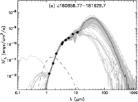
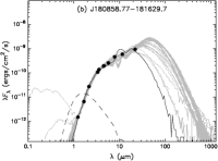
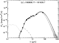
Figure 8.— Example of the fitting of models to an object. The filled circles and triangle symbolize the input fluxes and the upper limit, respectively. The black line shows the best fit. The gray lines show a set of fits that satisfy $\chi^{2}-\chi_{best}^{2}<2\times N_{data}$. The dashed line means the stellar photosphere corresponding to the central source of the best fitting model as it would look in the absence of circumstellar dust but with interstellar extinction. The panels (a)-(c) show the resulting SED fittings without the input fluxes at 24 and 70 $\mu$m, with the input flux at 24 $\mu$m, and with the input fluxes at 24 and 70 $\mu$m, respectively. The panel (d) is to check whether the source cannot be fit simply by a star with interstellar extinction.

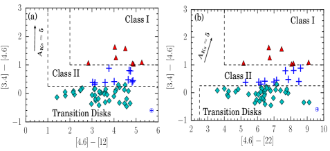
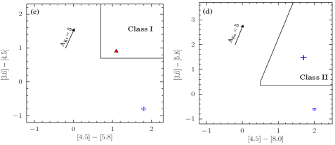
Figure 9.— Color-color diagrams for (a) WISE bands 1, 2, and 3; (b) WISE bands 1, 2, and 4; (c) IRAC bands 1, 2, and 3; (d) IRAC bands 1, 2, 3, and 4. Red triangles symbolize Class I YSOs, blue pluses Class II YSOs, and cyan diamond transition disk YSOs. The arrows show an extinction vector of $A_{\mathrm{K}}$ = 5 mag following the extinction laws of Koenig & Leisawitz (2014); Flaherty et al. (2007). The combined measurement errors are shown on the bottom right.

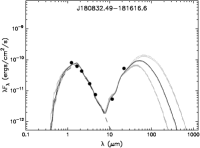
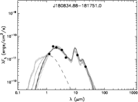
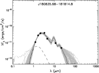
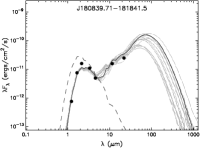
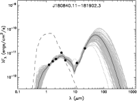
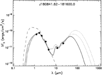
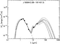
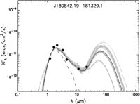
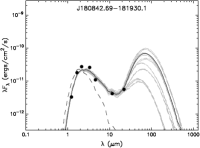
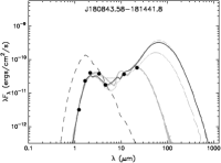
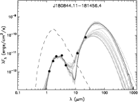
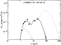
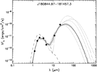
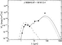
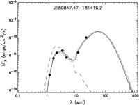
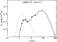
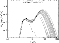
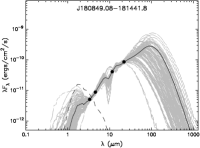
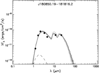
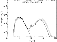
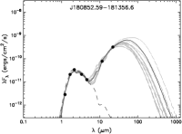
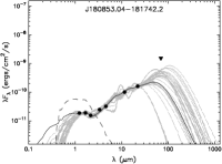
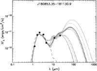
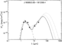
Figure 10.— SED fitting of candidate YSOs. The filled circles and triangle symbolize the input fluxes and the upper limit, respectively. The black line shows the best fit. The grey lines show a set of fits that satisfy $\chi^{2}-\chi_{best}^{2}<2\times N_{\mathrm{data}}$. The dashed line means the stellar photosphere corresponding to the central source of the best fitting model, as it would look in the absence of circumstellar dust but with interstellar extinction.

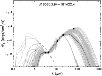
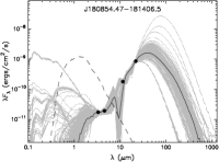
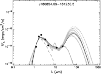
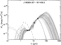
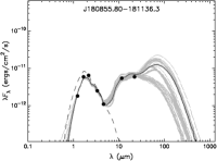
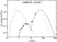
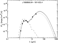
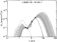
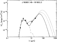
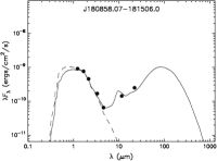
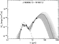
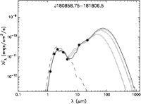
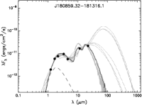
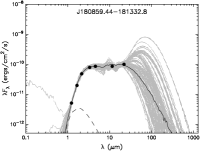
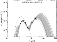
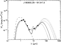
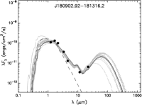
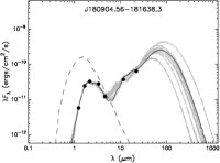
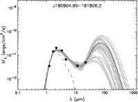
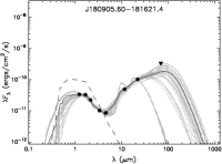
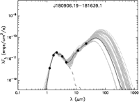
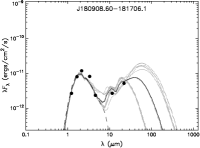
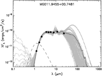
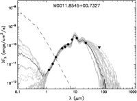
Figure 11.— – continued.

References

- Allen et al. (2004) Allen, L. E., Calvet, N., D’Alessio, P., et al. 2004, ApJS, 154, 363
- Anderson et al. (2012) Anderson, L. D., Zavagno, A., Deharveng, L., et al. 2012, A&A, 542, A10
- André et al. (2011) André, P., Men’shchikov, A., Könyves, V., & Arzoumanian, D. 2011, Computational Star Formation, 270, 255
- Beaumont & Williams (2010) Beaumont, C. N., & Williams, J. P. 2010, ApJ, 709, 791
- Beckwith et al. (1990) Beckwith, S. V. W., Sargent, A. I., Chini, R. S., & Guesten, R. 1990, AJ, 99, 924
- Benjamin et al. (2003) Benjamin, R. A., Churchwell, E., Babler, B. L., et al. 2003, PASP, 115, 953
- Bertoldi (1989) Bertoldi, F. 1989, ApJ, 346, 735
- Beuther et al. (2002) Beuther, H., Walsh, A., Schilke, P., et al. 2002, A&A, 390, 289
- Bisbas et al. (2011) Bisbas, T. G., Wünsch, R., Whitworth, A. P., Hubber, D. A., & Walch, S. 2011, ApJ, 736, 142
- Carey et al. (2009) Carey, S. J., Noriega-Crespo, A., Mizuno, D. R., et al. 2009, PASP, 121, 76
- Chen et al. (2010) Chen, X., Shen, Z.-Q., Li, J.-J., Xu, Y., & He, J.-H. 2010, ApJ, 710, 150
- Churchwell et al. (2006) Churchwell, E., Povich, M. S., Allen, D., et al. 2006, ApJ, 649, 759
- Churchwell et al. (1978) Churchwell, E., Smith, L. F., Mathis, J., Mezger, P. G., & Huchtmeier, W. 1978, A&A, 70, 719
- Churchwell et al. (2007) Churchwell, E., Watson, D. F., Povich, M. S., et al. 2007, ApJ, 670, 428
- Codella et al. (2004) Codella, C., Lorenzani, A., Gallego, A. T., Cesaroni, R., & Moscadelli, L. 2004, A&A, 417, 615
- Cyganowski et al. (2008) Cyganowski, C. J., Whitney, B. A., Holden, E., et al. 2008, AJ, 136, 2391
- Dale et al. (2007) Dale, J. E., Bonnell, I. A., & Whitworth, A. P. 2007, MNRAS, 375, 1291
- Dale et al. (2013) Dale, J. E., Ercolano, B., & Bonnell, I. A. 2013, MNRAS, 431, 1062
- Dale et al. (2015) Dale, J. E., Haworth, T. J., & Bressert, E. 2015, arXiv:1502.05865
- Deharveng et al. (2008) Deharveng, L., Lefloch, B., Kurtz, S., et al. 2008, A&A, 482, 585
- Deharveng et al. (2006) Deharveng, L., Lefloch, B., Massi, F., et al. 2006, A&A, 458, 191
- Deharveng et al. (2003) Deharveng, L., Lefloch, B., Zavagno, A., et al. 2003, A&A, 408, L25
- Deharveng et al. (2010) Deharveng, L., Schuller, F., Anderson, L. D., et al. 2010, A&A, 523, A6
- Deharveng et al. (2005) Deharveng, L., Zavagno, A., & Caplan, J. 2005, A&A, 433, 565
- Deharveng et al. (2009) Deharveng, L., Zavagno, A., Schuller, F., et al. 2009, A&A, 496, 177
- Dyson & Williams (1980) Dyson, J. E., & Williams, D. A. 1980, New York, Halsted Press, 1980. 204 p.,
- Elmegreen (2011) Elmegreen, B. G. 2011, EAS Publications Series, 51, 45
- Elmegreen & Lada (1977) Elmegreen, B. G., & Lada, C. J. 1977, ApJ, 214, 725
- Federrath et al. (2008) Federrath, C., Klessen, R. S., & Schmidt, W. 2008, ApJ, 688, L79
- Federrath et al. (2010) Federrath, C., Roman-Duval, J., Klessen, R. S., Schmidt, W., & Mac Low, M.-M. 2010, A&A, 512, A81
- Flaherty et al. (2007) Flaherty, K. M., Pipher, J. L., Megeath, S. T., et al. 2007, ApJ, 663, 1069
- Forster & Caswell (1999) Forster, J. R., & Caswell, J. L. 1999, A&AS, 137, 43
- Goldsmith & Langer (1999) Goldsmith, P. F., & Langer, W. D. 1999, ApJ, 517, 209
- Green et al. (2010) Green, J. A., Caswell, J. L., Fuller, G. A., et al. 2010, MNRAS, 409, 913
- Griffin et al. (2010) Griffin, M. J., Abergel, A., Abreu, A., et al. 2010, A&A, 518, L3
- Guilloteau & Lucas (2000) Guilloteau, S., & Lucas, R. 2000, Imaging at Radio through Submillimeter Wavelengths, 217, 299
- Gutermuth et al. (2009) Gutermuth, R. A., Megeath, S. T., Myers, P. C., et al. 2009, ApJS, 184, 18
- Gutermuth et al. (2008) Gutermuth, R. A., Myers, P. C., Megeath, S. T., et al. 2008, ApJ, 674, 336
- Guzmán et al. (2011) Guzmán, V., Pety, J., Goicoechea, J. R., Gerin, M., & Roueff, E. 2011, A&A, 534, A49
- Helfand et al. (2006) Helfand, D. J., Becker, R. H., White, R. L., Fallon, A., & Tuttle, S. 2006, AJ, 131, 2525
- Hill et al. (2005) Hill, T., Burton, M. G., Minier, V., et al. 2005, MNRAS, 363, 405
- Hosokawa & Inutsuka (2006) Hosokawa, T., & Inutsuka, S.-i. 2006, ApJ, 646, 240
- Hosokawa & Inutsuka (2005) Hosokawa, T., & Inutsuka, S.-i. 2005, ApJ, 623, 917
- Kang et al. (2009) Kang, M., Bieging, J. H., Povich, M. S., & Lee, Y. 2009, ApJ, 706, 83
- Kauffmann et al. (2008) Kauffmann, J., Bertoldi, F., Bourke, T. L., Evans, N. J., II, & Lee, C. W. 2008, A&A, 487, 993
- Kauffmann & Pillai (2010) Kauffmann, J., & Pillai, T. 2010, ApJ, 723, L7
- Kendrew et al. (2012) Kendrew, S., Simpson, R., Bressert, E., et al. 2012, ApJ, 755, 71
- Kim et al. (2011) Kim, K.-T., Byun, D.-Y., Je, D.-H., et al. 2011, Journal of Korean Astronomical Society, 44, 81
- Koenig et al. (2012) Koenig, X. P., Leisawitz, D. T., Benford, D. J., et al. 2012, ApJ, 744, 130
- Koenig & Leisawitz (2014) Koenig, X. P., & Leisawitz, D. T. 2014, ApJ, 791, 131
- Kurtz et al. (1994) Kurtz, S., Churchwell, E., & Wood, D. O. S. 1994, ApJS, 91, 659
- Kurtz et al. (2004) Kurtz, S., Hofner, P., & Álvarez, C. V. 2004, ApJS, 155, 149
- Kwan (1997) Kwan, J. 1997, ApJ, 489, 284
- Lada (1987) Lada, C. J. 1987, Star Forming Regions, 115, 1
- Lefloch & Lazareff (1994) Lefloch, B., & Lazareff, B. 1994, A&A, 289, 559
- Li et al. (2013) Li, J.-Y., Jiang, Z.-B., Liu, Y., & Wang, Y. 2013, Research in Astronomy and Astrophysics, 13, 921
- Liu et al. (2015) Liu, H.-L., Wu, Y., Li, J., et al. 2015, ApJ, 798, 30
- Liu et al. (2012) Liu, T., Wu, Y., Zhang, H., & Qin, S.-L. 2012, ApJ, 751, 68
- Lockman (1989) Lockman, F. J. 1989, ApJS, 71, 469
- Lumsden et al. (2013) Lumsden, S. L., Hoare, M. G., Urquhart, J. S., et al. 2013, ApJS, 208, 11
- Mueller et al. (2002) Mueller, K. E., Shirley, Y. L., Evans, N. J., II, & Jacobson, H. R. 2002, ApJS, 143, 469
- Markwardt (2009) Markwardt, C. B. 2009, Astronomical Data Analysis Software and Systems XVIII, 411, 251
- Martins et al. (2005) Martins, F., Schaerer, D., & Hillier, D. J. 2005, A&A, 436, 1049
- Martins et al. (2010) Martins, F., Pomarès, M., Deharveng, L., Zavagno, A., & Bouret, J. C. 2010, A&A, 510, A32
- Miao et al. (2006) Miao, J., White, G. J., Nelson, R., Thompson, M., & Morgan, L. 2006, MNRAS, 369, 143
- Miao et al. (2009) Miao, J., White, G. J., Thompson, M. A., & Nelson, R. P. 2009, ApJ, 692, 382
- Molinari et al. (2011) Molinari, S., Schisano, E., Faustini, F., et al. 2011, A&A, 530, A133
- Motte et al. (2007) Motte, F., Bontemps, S., Schilke, P., et al. 2007, A&A, 476, 1243
- Ogura (2010) Ogura, K. 2010, Astronomical Society of India Conference Series, 1, 19
- Offner et al. (2012) Offner, S. S. R., Robitaille, T. P., Hansen, C. E., McKee, C. F., & Klein, R. I. 2012, ApJ, 753, 98
- Paron et al. (2015) Paron, S., Ortega, M. E., Dubner, G., et al. 2015, AJ, 149, 193
- Poglitsch et al. (2010) Poglitsch, A., Waelkens, C., Geis, N., et al. 2010, A&A, 518, L2
- Povich et al. (2009) Povich, M. S., Churchwell, E., Bieging, J. H., et al. 2009, ApJ, 696, 1278
- Povich et al. (2013) Povich, M. S., Kuhn, M. A., Getman, K. V., et al. 2013, ApJS, 209, 31
- Purcell et al. (2013) Purcell, C. R., Hoare, M. G., Cotton, W. D., et al. 2013, ApJS, 205, 1
- Quireza et al. (2006) Quireza, C., Rood, R. T., Bania, T. M., Balser, D. S., & Maciel, W. J. 2006, ApJ, 653, 1226
- Reach et al. (2009) Reach, W. T., Faied, D., Rho, J., et al. 2009, ApJ, 690, 683
- Robitaille et al. (2006) Robitaille, T. P., Whitney, B. A., Indebetouw, R., Wood, K., & Denzmore, P. 2006, ApJS, 167, 256
- Robitaille et al. (2007) Robitaille, T. P., Whitney, B. A., Indebetouw, R., & Wood, K. 2007, ApJS, 169, 328
- Sadavoy et al. (2013) Sadavoy, S. I., Di Francesco, J., Johnstone, D., et al. 2013, ApJ, 767, 126
- Samal et al. (2014) Samal, M. R., Zavagno, A., Deharveng, L., et al. 2014, A&A, 566, A122
- Schneider et al. (2012) Schneider, N., Csengeri, T., Hennemann, M., et al. 2012, A&A, 540, L11
- Shirley (2015) Shirley, Y. L. 2015, PASP, 127, 299
- Skrutskie et al. (2006) Skrutskie, M. F., Cutri, R. M., Stiening, R., et al. 2006, AJ, 131, 1163
- Spitzer (1978) Spitzer, L. 1978, New York Wiley-Interscience, 1978. 333 p.,
- Thompson et al. (2012) Thompson, M. A., Urquhart, J. S., Moore, T. J. T., & Morgan, L. K. 2012, MNRAS, 421, 408
- Traficante et al. (2011) Traficante, A., Calzoletti, L., Veneziani, M., et al. 2011, MNRAS, 416, 2932
- Tremblin et al. (2012a) Tremblin, P., Audit, E., Minier, V., & Schneider, N. 2012a, A&A, 538, A31
- Tremblin et al. (2012b) Tremblin, P., Audit, E., Minier, V., Schmidt, W., & Schneider, N. 2012b, A&A, 546, A33
- Tremblin et al. (2014) Tremblin, P., Schneider, N., Minier, V., et al. 2014, A&A, 564, A106
- Urquhart et al. (2008) Urquhart, J. S., Hoare, M. G., Lumsden, S. L., Oudmaijer, R. D., & Moore, T. J. T. 2008, Massive Star Formation: Observations Confront Theory, 387, 381
- van der Wiel et al. (2009) van der Wiel, M. H. D., van der Tak, F. F. S., Ossenkopf, V., et al. 2009, A&A, 498, 161
- van der Wiel et al. (2010) van der Wiel, M. H. D., van der Tak, F. F. S., Ossenkopf, V., et al. 2010, A&A, 510, C1
- Vazquez-Semadeni (1994) Vazquez-Semadeni, E. 1994, ApJ, 423, 681
- Vázquez-Semadeni et al. (2008) Vázquez-Semadeni, E., González, R. F., Ballesteros-Paredes, J., Gazol, A., & Kim, J. 2008, MNRAS, 390, 769
- Watson et al. (2010) Watson, C., Hanspal, U., & Mengistu, A. 2010, ApJ, 716, 1478
- Whitney et al. (2004) Whitney, B. A., Indebetouw, R., Bjorkman, J. E., & Wood, K. 2004, ApJ, 617, 1177
- Whitworth et al. (1994) Whitworth, A. P., Bhattal, A. S., Chapman, S. J., Disney, M. J., & Turner, J. A. 1994, MNRAS, 268, 291
- Wink et al. (1983) Wink, J. E., Wilson, T. L., & Bieging, J. H. 1983, A&A, 127, 211
- Wright et al. (2010) Wright, E. L., Eisenhardt, P. R. M., Mainzer, A. K., et al. 2010, AJ, 140, 1868
- Wu et al. (2007) Wu, Y., Henkel, C., Xue, R., Guan, X., & Miller, M. 2007, ApJ, 669, L37
- Yuan et al. (2014) Yuan, J.-H., Wu, Y., Li, J. Z., & Liu, H. 2014, ApJ, 797, 40
- Zavagno et al. (2010) Zavagno, A., Anderson, L. D., Russeil, D., et al. 2010, A&A, 518, L101
- Zavagno et al. (2006) Zavagno, A., Deharveng, L., Comerón, F., et al. 2006, A&A, 446, 171
- Zavagno et al. (2007) Zavagno, A., Pomarès, M., Deharveng, L., et al. 2007, A&A, 472, 835