Non-Abelian topological spin liquids from arrays of quantum wires or spin chains

Abstract

We construct two-dimensional non-Abelian topologically ordered states by strongly coupling arrays of one-dimensional quantum wires via interactions. In our scheme, all charge degrees of freedom are gapped, so the construction can use either quantum wires or quantum spin chains as building blocks, with the same end result. The construction gaps the degrees of freedom in the bulk, while leaving decoupled states at the edges that are described by conformal field theories (CFT) in $(1+1)$-dimensional space and time. We consider both the cases where time-reversal symmetry (TRS) is present or absent. When TRS is absent, the edge states are chiral and stable. We prescribe, in particular, how to arrive at all the edge states described by the unitary CFT minimal models with central charges $c<1$. These non-Abelian spin liquid states have vanishing quantum Hall conductivities, but non-zero thermal ones. When TRS is present, we describe scenarios where the bulk state can be a non-Abelian, non-chiral, and gapped quantum spin liquid, or a gapless one. In the former case, we find that the edge states are also gapped. The paper provides a brief review of non-Abelian bosonization and affine current algebras, with the purpose of being self-contained. To illustrate the methods in a warm-up exercise, we recover the ten-fold way classification of two-dimensional non-interacting topological insulators using the Majorana representation that naturally arises within non-Abelian bosonization. Within this scheme, the classification reduces to counting the number of null singular values of a mass matrix, with gapless edge modes present when left and right null eigenvectors exist.

I Introduction

I.1 Motivation and strategy

Topologically ordered states of matter, Wen (1991a) of which the fractional quantum Hall effect (FQHE) is the quintessential example, contain rich elementary excitations. A necessary and sufficient condition for topological order is argued in Ref. Oshikawa and Senthil, 2006 to be the existence of point-like excitations obeying either Abelian Leinaas and Myrheim (1977); Wilczek (1982) or non-Abelian Fröhlich (1988); Fröhlich and Gabbiani (1990); Fröhlich et al. (1990); Rehren (1990); J. Fröhlich and P.A. Marchetti (1991); Moore and Read (1991); Wen (1991b); Kitaev (2006); Nayak et al. (2008) anyonic statistics.

The quantum numbers of the topological anyon excitations are encoded by a topological quantum field theory (TQFT) in the bulk. The type of TQFT in the bulk can imply the existence of gapless degrees of freedom on the edge, in the form of a conformal field theory (CFT) in $(1+1)$-dimensional space and time. While the bulk-boundary correspondence is not one-to-one, certain implications can be formulated. For example, the fractional part of the central charge Kitaev (2006) of the bulk TQFT has to match that of the chiral central charge of the edge CFT. (Changes by integers can always be obtained by gluing an integer-quantum-Hall-type phase to the $(2+1)$-dimensional system, which does not change the bulk TQFT.) Thus, the CFT describing the edge excitations is to some extend a diagnostic of the bulk topological order. For instance, the value taken by the central charge of this CFT is sensitive to whether it originates from either an Abelian or a non-Abelian topological order. A non-integer chiral central charge of the edge CFT implies non-Abelian topological order in the bulk.

The goal of this paper is to establish that a class of models built out of itinerant electrons, confined to two-dimensional space, display non-Abelian topological order upon fine-tuning of finite-range electron-electron interactions. The strategy that we employ is to couple a one-dimensional array of quantum wires, each of which supports a finite density of noninteracting electrons, through electron tunneling and electron-electron interactions. Prior to switching on the electron tunneling and electron-electron interactions, the electrons can only move ballistically along their hosting wire. There is no electronic motion in the direction transverse to any given wire. The one-dimensional array of quantum wires realizes a CFT in $(1+1)$-dimensional space and time with a central charge $c^{\,}_{\mathrm{decoupled}}$ twice the number of wires. After switching on the electron tunneling and electron-electron interactions, a crossover to two-dimensional physics takes place along which the noninteracting critical theory flows to a CFT with a central charge $c^{\,}_{\mathrm{coupled}}$ that is either zero or has a nonvanishing fractional part depending on whether periodic or open boundary conditions are imposed when coupling the wires. With periodic boundary conditions along the chain of wires, the ground state is separated from all excitations by a gap. With open boundary conditions along the chain of wires, the residual gapless excitations are necessarily localized along the left and right terminations of the chain of wires.

In our scheme, the charge degrees of freedom are gapped. For this reason, instead of using quantum wires as building blocks, we could equally as well start with a set of coupled quantum spin chains. This opens the possibility to engineer two-dimensional non-Abelian quantum spin liquids using coupled spin chains. We consider both the cases where time-reversal symmetry (TRS) is present or absent. The fact that we gap the charge degrees of freedom means that, even when time-reversal symmetry (TRS) is broken, there is no quantum Hall conductance, but only a quantum thermal Hall conductance; this is an example of a non-Abelian chiral spin liquid.

I.2 Summary of main results

We employ non-Abelian bosonization in order to construct symmetry protected topological (SPT) phases and topologically ordered phases of matter out of arrays of interacting quantum wires for, as the name suggests, non-Abelian bosonization is ideally suited to construct topological orders that are characterized by a non-Abelian Lie group.

The logic behind our construction is as follows. An individual quantum wire with spinful electrons has (in absence of spin-orbit or Zeeman couplings) an internal symmetry group $U^{\,}_{\mathrm{R}}(2)\times U^{\,}_{\mathrm{L}}(2)$, where R and L stands for the right-moving and left-moving modes at low energies, respectively. A translationally invariant array of $N$ such wires has the symmetry group $U^{\,}_{\mathrm{R}}(2N)\times U^{\,}_{\mathrm{L}}(2N)$. The generators of this group and any of its subgroups can be associated with current operators, which in turn are products of electron operators. Consider any subgroup $H$ of $U(2N)$. The degrees of freedom that are not singlets under the subgroup can be removed from $U^{\,}_{\mathrm{R}}(2N)$ and $U^{\,}_{\mathrm{L}}(2N)$ simultaneously via the interaction

$$\lambda^{\,}_{H}\sum_{a}\hat{J}^{a}_{\mathrm{R}}\,\hat{J}^{a}_{\mathrm{L}},\qquad\lambda^{\,}_{H}>0,$$ (1)

where $a$ runs over all generators of the subgroup $H$, while $\hat{J}^{a}_{\mathrm{R}}$ and $\hat{J}^{a}_{\mathrm{L}}$ are the associated current operators formed from the left-moving and right-moving modes respectively. The resulting theory will have a reduced number of degrees of freedom associated with the group quotient (or coset in short) $\left[U^{\,}_{\mathrm{R}}(2N)/H^{\,}_{\mathrm{R}}\right]\times\left[U^{\,}_{\mathrm{L}}(2N)/H^{\,}_{\mathrm{L}}\right]$.

When choosing possible subgroups $H$, the physical constraint of locality has to be observed. If the generators of $H$ involve electronic degrees of freedom from far apart wires, then $H$ is not admissible. Likewise, while $H^{\,}_{\mathrm{R}}$ and $H^{\,}_{\mathrm{L}}$ are the same mathematical subgroup, they need not be realized in the same wires. However, they need to be realized in nearby wires, as interaction (1) would otherwise represent long-range interactions between the wires.

The above procedure is then iterated using the same subgroup $H$ repeatedly, but each time realized on a different set of wires, until the symmetry group $U^{\,}_{\mathrm{R}}(2N)\times U^{\,}_{\mathrm{L}}(2N)$ is completely broken in the bulk. Physically this corresponds to gapping all the low-energy modes in the bulk. In an array of wires with open boundary conditions, there may remain a protected group coset with associated currents that are build exclusively from the degrees of freedom near the edge. For this procedure to be applicable, $H$ must be chosen such that $U^{\,}_{\mathrm{R}}(2N)/H^{\,}_{\mathrm{R}}$ still contains $H^{\,}_{\mathrm{R}}$ (shifted by the appropriate number of wires) as a subgroup, and likewise for L. This is a fundamental compatibility condition that has to be obeyed by all the current-current interactions that are used to gap out degrees of freedom. It is tantamount to the condition that the respective Hamiltonian terms of the form (1) commute.

Before embarking on this program, we choose in Sec. II.4 to employ as a warmup the non-Abelian bosonization technique to construct the noninteracting SPT phases that constitute the tenfold way for noninteracting topological insulators and superconductors, (the tenfold way, in short).  Schnyder et al. (2009); Kitaev (2009); Schnyder et al. (2008); Ryu et al. (2010) At first sight, this might seem to overcomplicate matters as the same result has already been obtained with Abelian bosonization.    Neupert et al. (2014) However, the essential case of the superconducting class D, stabilized by $\mathbb{Z}^{\,}_{2}$ fermion parity symmetry only, is at odds with the $U(1)$ group that is fundamentally associated with Abelian bosonization. One needs to invoke further arguments to obtain the desired construction.    Neupert et al. (2014) With non-Abelian bosonization, the construction follows rather naturally, as we shall see.

The symmetry group associated with the mean-field description of an array of $N$ (spinless) superconducting wires is $O^{\,}_{\mathrm{R}}(2N)\times O^{\,}_{\mathrm{L}}(2N)\sim U^{\,}_{\mathrm{R}}(N)\times U^{\,}_{\mathrm{L}}(N)$, where the right-moving and left-moving electronic degrees of freedom are each decomposed in two Majorana fermions. Via non-Abelian bosonization, these degrees of freedom are represented by a $O(2N)$-valued bosonic matrix field $G(t,x)$ that is a function of time $t$ and the position $x$ along the wire. A term

$$\lambda^{\,}_{M}\mathrm{tr}\,(G\,M),$$ (2)

parametrized by a constant and real-valued $2N\times 2N$ matrix $M$ gaps out all the modes that are not in the kernel of $M$. More precisely, the remaining right-moving Majorana modes correspond to the right eigenspace with eigenvalue $0$ of $M$, while the remaining left-moving Majoranas are the left eigenspace with eigenvalue 0. For example, if

$$M=\begin{pmatrix}0&\cdots&&0\\ 1&\ddots&&\\ &\ddots&&\\ 0&\cdots&1&0\end{pmatrix}$$ (3)

there remains a single left-moving Majorana mode at the left edge and a single right-moving Majorana mode at the right edge of the wire array. This realizes the simplest nontrivial example of an SPT state in class D, equivalent to a chiral $p$-wave superconductor.  Read and Green (2000); Ivanov (2001) We discuss all nontrivial examples from the tenfold way using this approach.

We then return in Sec. III to the main part of the paper, namely to intrinsically interacting and topologically ordered states of quantum wires. For this construction, we consider the subgroup $\cdots U(2k)\times U(2k^{\prime})\times U(2k)\times U(2k^{\prime})\cdots$ of the group $U(2N)$ of all wires by arranging $k$ and $k^{\prime}$ wires into a bundle in an alternating fashion. Then, the low-energy sector of each bundle is reduced to the states generated by the nontwisted affine Lie algebra $\widehat{su}^{\,}(2)^{\,}_{k}$ [and $\widehat{su}(2)^{\,}_{k^{\prime}}$ respectively]. This is achieved through current-current interactions from the coset representation

$$\widehat{su}(2)^{\,}_{k}=\frac{\widehat{u}(2k)}{\widehat{u}(1)\oplus\widehat{su}(k)^{\,}_{2}}.$$ (4)

The identity (4) is valid for any integer $k=1,2,\cdots$. Here, the $U(1)$ subgroup corresponds to the total charge of the electron modes in the $k$ consecutive wires of a bundle. To gap only this subgroup without gapping the charge mode of, e.g., a single wire, a $(2k)$-body interaction is used. In contrast, all the remaining interactions of the construction are of two-body nature. For example, the $\widehat{su}(k)^{\,}_{2}$ subalgebra in Eq. (4) corresponds to $k$ flavors within each bundle and is gapped by the respective current-current interactions. (The same applies to the other $k^{\prime}$ flavors within each bundle.) While these wire flavors in each bundle can be thought of as a pseudo- or isospin degree of freedom, the remaining nontwisted affine Lie algebra $\cdots\widehat{su}(2)^{\,}_{k}\oplus\widehat{su}(2)^{\,}_{k^{\prime}}\oplus\widehat{su}(2)^{\,}_{k}\oplus\widehat{su}(2)^{\,}_{k^{\prime}}\cdots$ stems from the physical spin of the electrons in the bundles of wires.

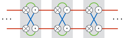
Figure 1: (Color online) Schematic representation of the Hamiltonian for a state with non-Abelian topological order arising from interactions between electronic quantum wires. Each $\otimes$ and $\odot$ represents the right-moving and left-moving (spinful) electrons of a quantum wire coming out of the plane of the page. Each gray area represents an interaction that gaps out charge fluctuations on the bundle of wires that it encloses. Each line represents a $SU(2)$ symmetric Heisenberg interaction between the spin densities of left-movers and right-movers that it connects. Lines of the same color represent interaction terms of the same strengths.

The essential step in our construction consists in coupling these coarse-grained $SU(2)$ “chiral spins” across the bundles of wires in such a way that a pattern of long-range entanglement emerges. This is achieved by coupling the right-moving subgroup in one wire bundle with the left-moving subgroup in the consecutive bundle with a current-current interaction. This coupling breaks time-reversal symmetry and makes our construction chiral. Our construction thus realizes a chiral spin liquid, not a fractional quantum Hall state (the Hall response vanishes). (A one-dimensional array of coupled spin-1/2 chains, if it is to support such a chiral spin-liquid ground state, must break time-reversal symmetry either explicitly or spontaneously.)

While gapping all modes in the bulk, there remains a right-moving (left-moving) coset-algebra $\widehat{su}(2)^{\,}_{k}\oplus\widehat{su}(2)^{\,}_{k^{\prime}}/\widehat{su}(2)^{\,}_{k+k^{\prime}}$ on the left (right) edge of the sample. It is protected, since it is fully chiral. This construction realizes, for different values of $k$ and $k^{\prime}$, edge states associated to different CFTs, with central charges $c^{\,}_{k,k^{\prime}}$. In particular, the associated CFTs on the edge include, for $k^{\prime}=1$, all unitary minimal models with central charge

$$c^{\,}_{k,1}= \,1-\frac{6}{(k+2)(k+3)}\;,$$ (5)

and, for $k^{\prime}=2$, all superconformal minimal models with central charge

$$c^{\,}_{k,2}=\frac{3}{2}-\frac{12}{(k+2)(k+4)}\;.$$ (6)

Figure 1 is a schematic illustration of the Hamiltonian that leads to the topologically ordered state for $k=k^{\prime}=1$, realizing Ising topological order.

We emphasize that the large non-Abelian symmetry group $U^{\,}_{\mathrm{R}}(2N)\times U^{\,}_{\mathrm{L}}(2N)$ that was invoked prior to coupling the wires should be thought of as a special limit that allows to use the tools of non-Abelian bosonization. It is not the symmetry $U^{\,}_{\mathrm{R}}(2N)\times U^{\,}_{\mathrm{L}}(2N)$ that is protecting the essential topological properties of the phase. It is worth noting that our construction preserves the full $SU(2)$ rotation symmetry of the physical spin. However, breaking it through the substitutions $\lambda^{\,}_{H}\to\lambda^{a}_{H}$ in Eq. (1) is inconsequential for the stability of the chiral edge states. Conversely, weakly breaking the full spin-1/2 $SU(2)$ rotation symmetry prior to coupling the wires is also inconsequential for the stability of the chiral edge states. (Weakly is defined relative to the characteristic energy scales involved in our $SU(2)$ symmetric construction of a topologically ordered phase.)

In the last parts of Sec. III, we investigate the consequences of imposing a symmetry acting trivially in space on such a wire construction. We study the case of time-reversal symmetry. One can define a time-reversal invariant system that is related to the chiral construction outlined above in one of two ways. (I) One adds to the Hamiltonian the time-reversed counterpart of each term that is already present. (II) One doubles the Hilbert space by invoking an additional valley degree of freedom that is exchanged under reversal of time and realizes in one valley the chiral construction outlined above and in the other valley its antichiral partner. Case (I) leads to a phase transition between two distinct topological ordered states that cannot be solved using non-Abelian bosonization. Case (II) is solvable by construction. It realizes a non-chiral and non-Abelian spin liquid. Since the charge sector is gapped both in the bulk and on the edges, the spin-Hall response vanishes. The edge of this system is nonchiral, as it hosts the chiral coset CFT in one valley polarization and the anti-chiral coset CFT in the other valley polarization on one given edge. It is then imperative to ask to what extend these edge-modes are stable against local time-reversal symmetric perturbations at the edge. We find that the edge is not stable. However, if a certain $U(1)$ symmetry is imposed, one-body backscattering terms are not sufficient to gap the edge. We determine the non-Abelian current-current interaction that is capable of gapping the edge in this case. This result is consistent with what is known from Abelian wire constructions in the case where a $U(1)$ subgroup of the $SU(2)$ spin-rotation symmetry is preserved. Protected edge modes appear only in phases with non-vanishing spin-Hall conductivity.  Neupert et al. (2011) (See also Ref. Scharfenberger et al., 2011 for a parton construction of non-Abelian spin liquids that respects time-reversal symmetry.)

I.3 Comparison with prior works

Arrays of coupled wires have been applied to many problems in statistical and in condensed matter physics.

The multi-channel Kondo effect can be formulated as an effective array of coupled quantum wires.  Affleck (1990); Affleck and Ludwig (1991a, b) We borrow the technology of conformal embedding from Refs. Affleck, 1990; Affleck and Ludwig, 1991a, b in this paper.

Another motivation to study coupled quantum wires stems from the mystery represented by the pseudogap phase in high-temperature superconductors and, more generally, the problem of the breakdown of Fermi liquid theory without conventional symmetry breaking.  Dagotto et al. (1992); Rice et al. (1993); Fabrizio (1993); Dagotto and Rice (1996); Balents and Fisher (1996); Lin et al. (1997); Carlson et al. (2000); Essler and Tsvelik (2002); Nersesyan and Tsvelik (2003); Starykh and Balents (2004); Jaefari et al. (2010) If each wire is half-filled and decoupled from all other wires, the charge sector is gapped while the spin-1/2 degrees of freedom are gapless. The decoupled array of quantum wires turns into a decoupled array of quantum spin-1/2 chains. Depending on how these spin-1/2 chains are coupled, gapped or gapless magnetic phases emerge in two and higher dimensions. Moving away from half-filling allows to study the correlated hopping of a small density of electrons or holes in a strongly correlated background of spins.

The bands of quasi-one-dimensional organic conductors such as the Bechgaard salts family are characterized by the hierarchy of electronic hopping amplitudes $t^{\,}_{a}\gg t^{\,}_{b}\gg t^{\,}_{c}$ along the orthogonal crystalline axis $a$, $b$, and $c$. This hierarchy justifies modeling the bands by weakly coupled quantum wires. In the presence of a uniform magnetic field parallel to the $c$ crystalline axis, the strongly nested Fermi surface is unstable to charge- or spin-density wave instabilities triggered by umklapp instabilities at a commensurate filling fraction. The limit, $t^{\,}_{c}/t^{\,}_{b}=0$ realizes the integer quantum Hall effect (IQHE).  Poilblanc et al. (1987); Yakovenko (1991) The limit, $t^{\,}_{c}/t^{\,}_{b}\ll 1$ realizes a weak topological insulator in the symmetry class A from the tenfold way.  Halperin (1987); Yakovenko (1991); Moore and Balents (2007)

The critical properties of the plateau transitions between two consecutive quantized Hall plateaus in the IQHE are captured by the Chalker-Coddington model (see Ref. Chalker and Coddington, 1988), in the limit in which electron-electron interactions are neglected. It was shown in Ref. Lee, 1994 how to represent the Chalker-Coddington model as a one-dimensional array of coupled quantum wires. More generally, one may assign to any array of quantum wires a transfer matrix that maps states that are incoming and outgoing to one end of the wires into states that are incoming and outgoing to the other end of the wires. This is a very useful approach to characterize analytically and numerically the effects of static disorder on transport along the wires, ignoring the effects of electron-electron interactions.

Coupling arrays of quantum wires by forward electronic interactions selects sliding Luttinger Liquid (SLL) phases in dimensions larger than one.  O’Hern et al. (1999); Emery et al. (2000); Vishwanath and Carpentier (2001); Mukhopadhyay et al. (2001); Sondhi and Yang (2001) In two remarkable papers, Refs. Kane et al., 2002 and Teo and Kane, 2014, it was shown how to add backward electronic interactions in a one-dimensional array of quantum wires so as to gap the SLL phases and stabilize Abelian and non-Abelian fractional quantum Hall states, respectively, instead (see also Refs. Klinovaja and Loss, 2014; Meng et al., 2014; Klinovaja and Tserkovnyak, 2014; Sagi and Oreg, 2014; Vaezi, 2014; Neupert et al., 2014; Meng and Sela, 2014; Klinovaja et al., 2015; Santos et al., 2015; Sagi et al., 2015 for one-dimensional arrays of coupled quantum wires and Ref. Meng, 2015 for a two-dimensional array of coupled quantum wires stabilizing long-ranged entangled phases of fermionic matter). Common to all these papers is the fact that only electron-electron interactions are considered, contrary to the models from Refs. Feiguin et al., 2007; Gils et al., 2009; Ludwig et al., 2011; Poilblanc et al., 2011; Mong et al., 2014; Sahoo et al., 2015; Hutter and Loss, 2015 in which the fundamental constituents are fractionalized fermions (such as Majorana fermions) subject to interactions.

What distinguishes our work from Ref. Teo and Kane, 2014 and ensuing papers is that we do not rely on the charge sector of the quantum wires to stabilize a non-Abelian topologically ordered phase. In Ref. Teo and Kane, 2014, the electrons are spin polarized by a strong uniform magnetic field, the filling fraction is fine tuned to the magnitude of the applied magnetic field. Here and as was done in Ref. Meng et al., 2015 when deriving Abelian and the $SU(2)$ level $k$ Read-Rezayi chiral spin liquids from arrays of quantum wires, we gap the charge sector from the outset by breaking translation invariance explicitly if necessary (i.e., if the filling fraction is not commensurate to the one-dimensional Fermi wave number), leaving only the spin-1/2 degrees of freedom in the low-energy sector of the theory. The non-Abelian topologically ordered phase is then selected by fine-tuned spin-spin interactions. When these interactions break time-reversal symmetry, the non-Abelian topologically ordered phase should be compared to the Abelian (see Refs. Kalmeyer and Laughlin, 1987; Wen et al., 1989; Mudry and Fradkin, 1989; Schroeter et al., 2007; Gong et al., 2014; Bauer et al., 2014; He and Chen, 2015; Hu et al., 2015; Gong et al., 2015; Gorohovsky et al., 2015; Kumar et al., 2015; Mei and Wen, 2014, 2015; Cincio and Qi, 2015; Bieri et al., 2015; He et al., 2015; Hu et al., 2015) and non-Abelian (see Refs. Greiter and Thomale, 2009; Greiter et al., 2014; Behrmann et al., 2015) chiral spin-liquid states that have been proposed for diverse two-dimensional lattices.

Common to Ref. Teo and Kane, 2014 is the belief that deriving topological ordered states from coupled wires is useful. First, it provides an intuitive bridge between the abstract description of topological order in terms of topological quantum field theories (see Ref. Wen, 2015 and references therein) on the one hand, and exactly solvable models that are designed from wave functions or lattice models that can only be studied numerically, on the other hand. Second, it opens the door for engineering materials supporting topological order.

II Review of Non-Abelian bosonization and current algebras

In order to keep this paper reasonably self-contained, we begin with a review on non-Abelian bosonization, including non-Abelian current algebras, which will be of major utility in deriving the main results of the paper in Sec. III. The reader who is fluent with non-Abelian bosonization is welcome to skip this brief summary and may jump to Sec. II.4, where, as a warmup exercise, we rederive the ten-fold classification of topological insulators in two-dimensional space using the tools here reviewed. A particular aspect in this section that is original is how to determine the presence of gapless edge modes in systems with boundaries, where we introduce a mass matrix whose null singular values signal gapless modes. Moreover, the left and right edge modes appear as left and right null eigenvectors of the mass matrix.

II.1 Affine Lie algebras

Non-Abelian bosonization is intimately related to affine Lie algebras. Affine Lie algebras are generalizations of Lie algebras.   Di Francesco et al. (1997) One of the Lie algebras with which physicists are most familiar is that associated to the total angular momentum operator $\hat{\bm{J}}$, i.e.,

$$[\hat{J}^{a},\hat{J}^{b}]=\sum_{c=1}^{3}\mathrm{i}\epsilon^{abc}\,\hat{J}^{c},\qquad a,b=1,2,3,$$ (7)

where we have set the Planck constant $\hbar$ to unity. The Levi-Civita symbol $\epsilon^{abc}$, the fully antisymmetric rank three tensor, is an example of the structure constants of a Lie algebra. The three components of the total angular momentum operator $\hat{\bm{J}}$ are the generators of the Lie algebra (7). This Lie algebra is denoted by $su(2)$, for the operator $\exp(\mathrm{i}\bm{\alpha}\cdot\hat{\bm{J}})$ represents an element of the unitary group $SU(2)$ parametrized by the vector $\bm{\alpha}\in\mathbb{R}^{3}$.

More generally, a Lie algebra $\mathfrak{g}$ is a vector space equipped with a binary operation denoted $[\cdot,\cdot]$ that is called the Lie bracket. The Lie bracket is a mapping from $\mathfrak{g}\times\mathfrak{g}\to\mathfrak{g}$ such that it is (i) antisymmetric under interchange of its two entries, (ii) linear in both entries, and (iii) satisfies the Jacobi identity

$$[X,[Y,Z]]+[Y,[Z,X]]+[Z,[X,Y]]=0$$ (8)

for any $X,Y,Z\in\mathfrak{g}$.

A Lie algebra can be specified by a set of generators $\hat{J}^{a}$ with $a=1,\cdots,\mathrm{dim}\,\mathfrak{g}$ that are Hermitian operators obeying the relations

$$[\hat{J}^{a},\hat{J}^{b}]=\sum_{c=1}^{\mathrm{dim}\,\mathfrak{g}}\mathrm{i}f^{ab}_{\hphantom{ab}c}\,\hat{J}^{c}$$ (9)

for $a,b=1,\cdots,\mathrm{dim}\,\mathfrak{g}$. The number $\mathrm{dim}\,\mathfrak{g}$ of generators is the dimension of the algebra. The numbers $f^{ab}_{\hphantom{ab}c}$ are real valued and can be chosen to be antisymmetric under interchange of $a$ and $b$ by virtue of the fact that the Lie bracket is antisymmetric under exchanging $a$ with $b$.

A subset $\mathfrak{h}$ of the Lie algebra $\mathfrak{g}$ is called a Lie subalgebra if this subset is closed under the Lie bracket, i.e., if $[\mathfrak{h},\mathfrak{h}]\subset\mathfrak{h}$. A Lie subalgebra $\mathfrak{h}$ of $\mathfrak{g}$ is an ideal if it satisfies the stronger constraint that $[\mathfrak{g},\mathfrak{h}]\subset\mathfrak{h}$. The null vector and $\mathfrak{g}$ itself are trivially ideals. A proper ideal of $\mathfrak{g}$ is an ideal that is neither the null vector nor $\mathfrak{g}$ itself. A simple Lie algebra has no proper ideal. A semisimple Lie algebra is a direct sum of simple Lie algebras. A semisimple Lie algebra generates a semisimple Lie group, i.e., a direct product of simple Lie groups.

Let $t$ be any real number and let $\mathbb{C}[t,t^{-1}]$ denote the set of polynomials of the form $\sum_{n\in\mathbb{Z}}p^{\,}_{n}\,t^{n}$ with finitely many nonvanishing complex-valued coefficients $p^{\,}_{n}$. Let $\mathfrak{g}$ denote a Lie algebra. The loop algebra

$$\tilde{\mathfrak{g}}:=\mathfrak{g}\otimes\mathbb{C}[t,t^{-1}]$$ (10a)

is a Lie algebra equipped with the Lie bracket

$$[\hat{J}^{a}_{m},\hat{J}^{b}_{n}]=\sum_{c=1}^{\mathrm{dim}\,\mathfrak{g}}\mathrm{i}f^{ab}_{\hphantom{ab}c}\,\hat{J}^{c}_{m+n},$$ (10b)

where the short-hand notation

$$\hat{J}^{a}_{m}:=\hat{J}^{a}\otimes t^{m},\quad\hat{J}^{b}_{n}:=\hat{J}^{b}\otimes t^{n},\quad\hat{J}^{c}_{m+n}:=\hat{J}^{c}\otimes t^{m+n},$$ (10c)

was introduced for any $a,b=1,\cdots,\mathrm{dim}\,\mathfrak{g}$ and for any $m,n\in\mathbb{Z}$.

Introduce the one-dimensional vector space

$$\mathbb{C}\hat{k}:=\{z\,\hat{k}\ |\ z\in\mathbb{C}\}.$$ (11)

Introduce the operator

$$\hat{L}^{\,}_{0}:=-t\frac{\mathrm{d}}{\mathrm{d}t}$$ (12a)

acting on the vector space of Laurent polynomials $$\mathbb{C}[t,t^{-1}]$$ through the operation of commutation with the fundamental rule that

$$\hat{L}^{\,}_{0}\,t^{m}-t^{m}\,\hat{L}^{\,}_{0}=-m\,t^{m}$$ (12b)

for any integer $$m$$ and define the one-dimensional vector space

$$\mathbb{C}\hat{L}^{\,}_{0}:=\{z\,\hat{L}^{\,}_{0}\ |\ z\in\mathbb{C}\}.$$ (12c)

The algebra

$$\hat{\mathfrak{g}}:=\tilde{\mathfrak{g}}\oplus\mathbb{C}\hat{k}\oplus\mathbb{C}\hat{L}^{\,}_{0}$$ (13a)

with the brackets

$$[\hat{J}^{a}_{m},\hat{J}^{b}_{n}]=\sum_{c=1}^{\mathrm{dim}\,\mathfrak{g}}\mathrm{i}f^{ab}_{\hphantom{ab}c}\,\hat{J}^{c}_{m+n}+\hat{k}\,n\,\delta^{ab}\,\delta^{\,}_{m+n,0},$$ (13b)

$$[\hat{J}^{a}_{m},\hat{L}^{\,}_{0}]=m\hat{J}^{a}_{m},$$ (13c)

and

$$[\hat{J}^{a}_{m},\hat{k}]=0$$ (13d)

for any $a,b=1,\cdots,\mathrm{dim}\,\mathfrak{g}$ and for any $m,n\in\mathbb{Z}$ is called a nontwisted affine Lie algebra. It is an infinite-dimensional algebra with the generators $\hat{J}^{a}_{m}$, $\hat{k}$, and $\hat{L}^{\,}_{0}$.

The simplest realization of an affine Lie algebra in physics is that of the normal modes $\hat{a}^{{\dagger}}_{m}$ and $\hat{a}^{\,}_{n}$ of the real-valued Klein-Gordon scalar field in $(1+1)$-dimensional Minkowski space and time. These obey the canonical Boson algebra

$$[\hat{a}^{\,}_{m},\hat{a}^{{\dagger}}_{n}]=\delta^{\,}_{m,n},\qquad[\hat{a}^{\,}_{m},\hat{a}^{\,}_{n}]=[\hat{a}^{{\dagger}}_{m},\hat{a}^{{\dagger}}_{n}]=0.$$ (14)

The Heisenberg algebra

$$[\hat{L}^{\,}_{m},\hat{L}^{\,}_{n}]=[\hat{R}^{\,}_{m},\hat{R}^{\,}_{n}]=m\,\delta^{\,}_{m+n,0},\qquad[\hat{L}^{\,}_{m},\hat{R}^{\,}_{n}]=0,$$ (15a)

for the nonvanishing integers $$m n$$ and follows from the definitions

$$\hat{L}^{\,}_{n}:=\begin{cases}-\mathrm{i}\sqrt{+n}\,\hat{a}^{\,}_{+n},&n>0,\\ +\mathrm{i}\sqrt{-n}\,\hat{a}^{{\dagger}}_{-n},&n<0,\end{cases}$$ (15b)

$$\hat{R}^{\,}_{n}:=\begin{cases}-\mathrm{i}\sqrt{+n}\,\hat{a}^{\,}_{-n},&n>0,\\ +\mathrm{i}\sqrt{-n}\,\hat{a}^{{\dagger}}_{+n},&n<0.\end{cases}$$ (15c)

The Heisenberg algebra is the affine extension of the $\hat{u}(1)$ algebra generated by the zero mode $\hat{a}^{\,}_{0}$. The eigenvalue of the central operator $\hat{k}$ is not quantized for an Abelian Lie group as it depends on the multiplicative factor chosen in the transformations (15b) and (15c).

II.2 Free fermion realizations of affine Lie algebras

We define the partition function

$$Z:=\int\mathcal{D}[\chi]\,e^{-S[\chi]}$$ (16a)

over the Grassmann vector field $$\chi^{\mathsf{T}}\equiv\begin{pmatrix}\chi^{\mathsf{T}}_{\mathrm{R}}&\chi^{\mathsf{T}}_{\mathrm{L}}\end{pmatrix}$$ with the action

$$S[\chi]:=\frac{\mathrm{i}}{2}\int\frac{\mathrm{d}\bar{z}\,\mathrm{d}z}{2}\left(\chi^{\mathsf{T}}_{\mathrm{R}}\,2\partial^{\,}_{\bar{z}}\,\chi^{\,}_{\mathrm{R}}+\chi^{\mathsf{T}}_{\mathrm{L}}\,2\partial^{\,}_{z}\,\chi^{\,}_{\mathrm{L}}\right)$$ (16b)

and the complex coordinates $\bar{z}=x^{\,}_{1}-\mathrm{i}x^{\,}_{2}$ and $z=x^{\,}_{1}+\mathrm{i}x^{\,}_{2}$ of the complex plane. (Choosing $x_{1}\equiv t$ and $x_{2}\equiv\mathrm{i}x$ relates the complex plane to $(1+1)$-dimensional Minkowski space and time.) The Grassmann vector field $\chi^{\mathsf{T}}_{\mathrm{R}}\equiv(\chi^{\,}_{\mathrm{R},1}\cdots\chi^{\,}_{\mathrm{R},n})$ only depends on $z$, it is holomorphic. The Grassmann vector field $\chi^{\mathsf{T}}_{\mathrm{L}}\equiv(\chi^{\,}_{\mathrm{L},1}\cdots\chi^{\,}_{\mathrm{L},n})$ only depends on $\bar{z}$, it is antiholomorphic. Their components obey the Laurent series expansion, i.e., the operator product expansion (OPE),

$$\chi^{\,}_{\mathrm{R},\alpha}(z)\,\chi^{\,}_{\mathrm{R},\beta}(0)=-\frac{\mathrm{i}}{2\pi}\,\frac{\delta^{\,}_{\alpha\beta}}{z}+\cdots,$$ (17a)

$$\chi^{\,}_{\mathrm{L},\alpha}(\bar{z})\,\chi^{\,}_{\mathrm{L},\beta}(0)=-\frac{\mathrm{i}}{2\pi}\,\frac{\delta^{\,}_{\alpha\beta}}{\bar{z}}+\cdots,$$ (17b)

$$\chi^{\,}_{\mathrm{R},\alpha}(z)\,\chi^{\,}_{\mathrm{L},\beta}(0)=0,$$ (17c)

for any $\alpha,\beta=1,\cdots,n$.

The theory (16) is invariant under the local transformation

$$\chi^{\,}_{\mathrm{R}}(z)\mapsto O^{\,}_{\mathrm{R}}(z)\,\chi^{\,}_{\mathrm{R}}(z),\qquad\chi^{\,}_{\mathrm{L}}(\bar{z})\mapsto O^{\,}_{\mathrm{L}}(\bar{z})\,\chi^{\,}_{\mathrm{L}}(\bar{z}),$$ (18)

where $O^{\,}_{\mathrm{R}}(z)$ and $O^{\,}_{\mathrm{L}}(\bar{z})$ are matrix fields belonging to $SO(n)$.

Define the corresponding $so(n)$ Noether currents

$$J^{a}(z):=\mathrm{i}\pi\,(\chi^{\mathsf{T}}_{\mathrm{R}}\,T^{a}\,\chi^{\,}_{\mathrm{R}})(z),\quad\bar{J}^{a}(\bar{z}):=\mathrm{i}\pi\,(\chi^{\mathsf{T}}_{\mathrm{L}}\,T^{a}\,\chi^{\,}_{\mathrm{L}})(\bar{z}),$$ (19a)

where the generators $$T^{a}\equiv T^{(rs)} a (r,s) 1\leq r<s\leq n n\times n$$ [with the collective label representing the ordered pair with ] are Hermitian matrices with the components

$$T^{(rs)}_{ij}=\mathrm{i}\left(\delta^{\,}_{r,i}\,\delta^{\,}_{s,j}-\delta^{\,}_{r,j}\,\delta^{\,}_{s,i}\right).$$ (19b)

It then follows that

$$J^{a}(z)\,J^{b}(0)=\sum_{c}\frac{\mathrm{i}f^{ab}_{\hphantom{ab}c}\,J^{c}(0)}{z}+\frac{1}{2}\frac{\mathrm{tr}\,(T^{a}\,T^{b})}{z^{2}},$$ (20a)

$$\bar{J}^{a}(\bar{z})\,\bar{J}^{b}(0)=\sum_{c}\frac{\mathrm{i}f^{ab}_{\hphantom{ab}c}\,\bar{J}^{c}(0)}{\bar{z}}+\frac{1}{2}\frac{\mathrm{tr}\,(T^{a}\,T^{b})}{\bar{z}^{2}},$$ (20b)

$$J^{a}(z)\,\bar{J}^{b}(0)=0,$$ (20c)

where

$$f^{ab}_{\hphantom{ab}c}\equiv \,f^{\,}_{(rs)(pq)(mn)}$$

$$= \,\delta^{\,}_{m,r}\left(\delta^{\,}_{n,q}\,\delta^{\,}_{s,p}-\delta^{\,}_{n,p}\,\delta^{\,}_{s,q}\right)$$

$$+\delta^{\,}_{m,s}\left(\delta^{\,}_{r,q}\,\delta^{\,}_{n,p}-\delta^{\,}_{n,q}\,\delta^{\,}_{r,p}\right)$$ (20d)

are the structure constants of $$so(n)$$. Observe that the choice made in Eq. (19b) implies the normalizations

$$\mathrm{tr}\,(T^{a}\,T^{b})=2\,\delta^{ab},\qquad\sum_{a,b}f^{ab}_{\hphantom{ab}c}\,f^{ab}_{\hphantom{ab}d}=2(n-2)\,\delta^{\,}_{cd}.$$ (20e)

Insertion of the Laurent expansions

$$J^{a}(z)=:\sum_{m\in\mathbb{Z}}z^{-m-1}\,J^{a}_{m},\qquad\bar{J}^{a}(z)=:\sum_{m\in\mathbb{Z}}\bar{z}^{-m-1}\,\bar{J}^{a}_{m},$$ (21)

into the operator product expansions (20a) and (20b), respectively, delivers a pair of a holomorphic and an antiholomorphic affine Lie algebra of the form (13) with the central term $\hat{k}$ replaced by its eigenvalue, the level $k=1$.

We close this discussion of free Majorana fermions with the definition of their central charge. Without loss of generality, we work in the holomorphic sector of the theory. The energy-momentum tensor has the light-cone component

$$T^{\,}_{\mathrm{R}}(z)\equiv \,-2\pi\,T^{\,}_{zz}$$

$$\equiv \,-\frac{\pi}{2}\,T^{\bar{z}\bar{z}}(z)$$

$$:= \,-\mathrm{i}\frac{\pi}{2}\sum_{\alpha=1}^{n}2\,\left(\frac{\delta S}{\delta(\partial^{\,}_{\bar{z}}\,\chi^{\,}_{\mathrm{R},\alpha})}(\partial^{\,}_{z}\chi^{\,}_{\mathrm{R},\alpha})\right)(z)$$

$$= \,\mathrm{i}\pi\left(\chi^{\mathsf{T}}_{\mathrm{R}}\,\partial^{\,}_{z}\,\chi^{\,}_{\mathrm{R}}\right)(z).$$ (22a)

Its OPE with itself is

$$T^{\,}_{\mathrm{R}}(z)\,T^{\,}_{\mathrm{R}}(0)=\frac{c/2}{z^{4}}+\frac{2\,T^{\,}_{\mathrm{R}}(0)}{z^{2}}+\frac{(\partial^{\,}_{z}T^{\,}_{\mathrm{R}})(0)}{z}+\cdots,$$ (22b)

where the numerator of the term with the fourth-order pole is

$$c=n/2.$$ (22c)

The number $c$ is called the central charge associated to the (holomorphic) Virasoro algebra defined by the OPE (22b).

II.3 Bosonic realizations of affine Lie algebras

Another example of a critical theory is the Wess-Zumino-Witten (WZW) model defined by the partition function   Wess and Zumino (1971); Witten (1984)

$$Z:=\int\limits\mathcal{D}[G]\,e^{-S^{\,}_{\mathrm{WZW}}[G]},$$ (23a)

where $$G\in\mathfrak{G} \mathfrak{G} \mathcal{D}[G] \mathfrak{G} \hat{\mathfrak{g}}^{\,}_{k} k \mathfrak{G} (x,y)\equiv(x^{\,}_{i})\in\mathbb{R}^{2}$$ denotes a matrix-valued bosonic field, denotes a compact Lie group, and denotes the Haar measure on . (We shall denote with the affine Lie algebra of integer level corresponding to the compact Lie group .) The WZW action in two-dimensional Euclidean space is

$$S^{\,}_{\mathrm{WZW}}[G]:=\frac{k}{16\pi}\int\mathrm{d}^{2}x\,\mathrm{tr}\left(\partial^{\,}_{i}G\,\partial^{\,}_{i}G^{-1}\right)+k\,\Gamma[G].$$ (23b)

(The summation convention over the repeated index $$i=1,2 \Gamma[G]$$ is implied.) The topological contribution is the Wess-Zumino term

$$\begin{split}\Gamma[G]:=&\,-\frac{\mathrm{i}}{24\pi}\int\limits_{B}\mathrm{d}^{3}\xi\,\epsilon^{ijk}\\ &\,\times\mathrm{tr}\Bigl{[}(\bar{G}^{-1}\partial^{\,}_{i}\bar{G})\,(\bar{G}^{-1}\partial^{\,}_{j}\bar{G})(\bar{G}^{-1}\partial^{\,}_{k}\bar{G})\Bigr{]}.\end{split}$$ (23c)

Here, $\bar{G}$ denotes the extension of $G$ to the solid ball $B\equiv\{(\xi^{\,}_{1},\xi^{\,}_{2},\xi^{\,}_{3})|\sum_{i=1}^{3}\xi^{2}_{i}\leq 1\}$ with two-dimensional Euclidean space as its boundary. As explained in Refs. Wess and Zumino, 1971; Witten, 1984, $k$ must be an integer for the functional $\exp(-k\,\Gamma[G])$ over the compact Lie group $\mathfrak{G}$ to be single valued.

The theory (23) is invariant under the local transformation

$$G(\bar{z},z)\mapsto L(\bar{z})\,G(\bar{z},z)\,R^{\mathsf{T}}(z),$$ (24)

where $R$ and $L$ are matrices belonging to $\mathfrak{G}$ and $\bar{z}=x-\mathrm{i}y$ is the complex conjugate to $z=x+\mathrm{i}y\in\mathbb{C}$. The OPE of its Noether currents (with proper normalizations) delivers a pair of a holomorphic and an antiholomorphic affine Lie algebra $\hat{\mathfrak{g}}^{\,}_{k}$ of the form (13) with the central term $\hat{k}$ replaced by its eigenvalue, the level $k$.

The central charge $c$ of the bosonic theory (23) is

$$c=\frac{k\,\mathrm{dim}(\mathfrak{G})}{k+\mathrm{Coxeter}^{\star}(\mathfrak{G})},$$ (25)

where $\mathrm{dim}(\mathfrak{G})$ is the dimension of the compact Lie group $\mathfrak{G}$ (the dimensionality of its adjoint representation), while $\mathrm{Coxeter}^{\star}(\mathfrak{G})$ is the dual Coxeter (twice the eigenvalue of the Casimir operator in the adjoint representation when the squared length of the highest root is normalized to 2).

If

$$\mathfrak{G}=\mathfrak{G}^{\,}_{1}\times\mathfrak{G}^{\,}_{2},$$ (26a)

it then follows that

$$c=\sum_{i=1,2}\frac{k\,\mathrm{dim}(\mathfrak{G}^{\,}_{i})}{k+\mathrm{Coxeter}^{\star}(\mathfrak{G}^{\,}_{i})}.$$ (26b)

More generally, denote with $\hat{\mathfrak{g}}^{(i)}_{k^{\,}_{i}}$ the WZW theory of level $k^{\,}_{i}$. The WZW theory with the semi-simple affine Lie algebra

$$\hat{\mathfrak{g}}:=\hat{\mathfrak{g}}^{(i)}_{k^{\,}_{1}}\oplus\cdots\oplus\hat{\mathfrak{g}}^{(i)}_{k^{\,}_{i}}\oplus\cdots$$ (27a)

has the central charge

$$c=\sum_{i}\frac{k^{\,}_{i}\,\mathrm{dim}(\mathfrak{G}^{(i)})}{k^{\,}_{i}+\mathrm{Coxeter}^{\star}(\mathfrak{G}^{(i)})}.$$ (27b)

There are several ways to make contact between the critical theory (16) and the critical theory (23).
Example 1: We do the identifications

$$\mathfrak{G}\to O(n),\qquad k\to 1,$$ (28a)

for which

$$\mathrm{dim}(\mathfrak{G})\to\frac{1}{2}\,n\,(n-1),$$ (28b)

$$\mathrm{Coxeter}^{\star}(\mathfrak{G})\to n-2,$$ (28c)

$$c=\frac{\mathrm{dim}(\mathfrak{G})}{1+\mathrm{Coxeter}^{\star}(\mathfrak{G})}$$

$$\hphantom{c}\,\to\frac{(1/2)\,n\,(n-1)}{1+n-2}$$

$$\hphantom{c}\,=\frac{1}{2}\,n.$$ (28d)

Example 2: We assume that $n=m\,n^{\prime}$ and do the identifications

$$\hat{\mathfrak{g}}\to\oplus_{i=1}^{n^{\prime}}\hat{\mathfrak{g}}^{\,}_{i},\qquad\mathfrak{G}^{\,}_{i}=O(m),\qquad k^{\,}_{i}\to 1,$$ (29a)

for which

$$\mathrm{dim}\,\mathfrak{G}^{\,}_{i}\to\frac{1}{2}\,m\,(m-1),$$ (29b)

$$\mathrm{Coxeter}^{\star}(\mathfrak{G}^{\,}_{i})\to m-2,$$ (29c)

$$c=\sum_{i=1}^{n^{\prime}}\frac{\mathrm{dim}(\mathfrak{G}^{\,}_{i})}{k^{\,}_{i}+\mathrm{Coxeter}^{\star}(\mathfrak{G}^{\,}_{i})}$$

$$\hphantom{c}\to n^{\prime}\frac{(1/2)\,m\,(m-1)}{1+m-2}$$

$$\hphantom{c}=\frac{1}{2}\,m\,n^{\prime}.$$ (29d)

This result for the central charge can be applied to the cases of $O(1)$ and $O(2)$ even though $O(1)$ is not a continuous Lie group while $O(2)$ is an Abelian group.

We choose Example 1. The non-Abelian bosonization rule for any local quadratic term made from the Majorana fields [$\chi^{\,}_{\mathrm{R}}$ ($\chi^{\,}_{\mathrm{L}}$) denotes the right-moving (left-moving) $n$-component Majorana vector field] is

$$m^{\,}_{\mathrm{uv}}\,G^{\,}_{\alpha\beta}=\mathrm{i}\chi^{\,}_{\mathrm{L},\alpha}\,\chi^{\,}_{\mathrm{R},\beta},$$ (30)

for $\alpha,\beta=1,\cdots,n$, and where $m^{\,}_{\mathrm{uv}}$ is the mass parameter that depends on the regularization scheme (the ultra-violet cutoff), and $G^{\,}_{\alpha\beta}$ is a matrix element of $G$.

The central charge of the $O(n)^{\,}_{1}$ WZW model is

$$c=\frac{n}{2}.$$ (31)

It coincides with the central charge for $n$ Majorana fermions (16), as the central charge of a single pair of right- and left-moving Majorana channels is $1/2$.

Recall that the central charge counts the effective degrees of freedom at criticality, i.e., the effective number of gapless degrees of freedom. Thus, if we add some quadratic mass term into our massless fermionic theory (16) so as to break a part of the $O(n)$ symmetry, the central charge should then be reduced.

For example, if we add the term

$$\mathrm{i}\chi^{\,}_{\mathrm{L},1}\,\chi^{\,}_{\mathrm{R},2}=m^{\,}_{\mathrm{uv}}\,G^{\,}_{12},$$ (32)

then the symmetry $O^{\,}_{\mathrm{R}}(n)\times O^{\,}_{\mathrm{L}}(n)$ breaks down to $O^{\,}_{\mathrm{R}}(n-1)\times O^{\,}_{\mathrm{L}}(n-1)$. Correspondingly, the central charge reduces to

$$c=\frac{n}{2}-\frac{1}{2}.$$ (33)

A pair of right- and left-moving Majorana modes has become massive.

Observe that

$$\mathrm{i}\chi^{\,}_{\mathrm{L},1}\,\chi^{\,}_{\mathrm{R},2}+\mathrm{i}\chi^{\,}_{\mathrm{L},1}\,\chi^{\,}_{\mathrm{R},3}=m^{\,}_{\mathrm{uv}}\,(G^{\,}_{12}+G^{\,}_{13})$$ (34)

does not reduce the $O^{\,}_{\mathrm{R}}(n)\times O^{\,}_{\mathrm{L}}(n)$ symmetry to $O^{\,}_{\mathrm{R}}(n-2)\times O^{\,}_{\mathrm{L}}(n-2)$. To see this, introduce the matrix $M$

$$G^{\,}_{12}+G^{\,}_{13}=:\mathrm{tr}(M\,G).$$ (35)

A solution is to choose a matrix with the only nonvanishing matrix elements $M^{\,}_{21}=M^{\,}_{31}=1$ sitting on the same column. This is to say that $M$ is constructed out of only one linearly independent column vector out of $n$ column vectors. Hence, there must exist two orthogonal matrices $R$ and $L$ such that

$$M^{\,}_{\mathrm{d}}=R^{\mathsf{T}}\,M\,L$$ (36)

is a diagonal matrix with one and only one nonvanishing diagonal matrix element. We choose this nonvanishing matrix element to be the first diagonal entry, $(M^{\,}_{\mathrm{d}})^{\,}_{11}=\Omega^{\,}_{1}\neq 0$. While the action (23) is invariant under the transformation (24), the mass term becomes

$$m^{\,}_{\mathrm{uv}}\mathrm{tr}(M\,G)\mapsto \,m^{\,}_{\mathrm{uv}}\,\mathrm{tr}(M\,L\,G^{\,}\,R^{\mathsf{T}})$$

$$= \,m^{\,}_{\mathrm{uv}}\,\mathrm{tr}(R^{\mathsf{T}}\,M\,L\,G^{\,})$$

$$= \,m^{\,}_{\mathrm{uv}}\,\mathrm{Tr}(M^{\,}_{\mathrm{d}}\,G^{\,})$$

$$= \,m^{\,}_{\mathrm{uv}}\,\Omega^{\,}_{1}\,G^{\,}_{11}$$

$$= \,\mathrm{i}\chi^{\,}_{\mathrm{L},1}\,\chi^{\,}_{\mathrm{R},1}$$ (37)

after the transformation (24). Hence, the mass term (34) reduces the symmetry to $O^{\,}_{\mathrm{R}}(n-1)\times O^{\,}_{\mathrm{L}}(n-1)$ and not to $O^{\,}_{\mathrm{R}}(n-2)\times O^{\,}_{\mathrm{L}}(n-2)$, as might have been erroneously deduced by identifying the “$2$” in $n-2$ with two independent mass terms.

For an arbitrary mass-matrix $M$, we can employ the singular-value decomposition

$$M^{\,}_{\mathrm{d}}=R^{\mathsf{T}}\,M\,L,$$ (38)

to get a diagonal matrix of rank $r$, i.e.,

$$M^{\,}_{\mathrm{diag}}=\mathrm{diag}\left(\underbrace{\Omega^{\,}_{1},\Omega^{\,}_{2},\cdots,\Omega^{\,}_{r}}^{\,}_{r},\underbrace{0,0,...,0}^{\,}_{n-r}\right),$$ (39)

whereby $\Omega^{\,}_{1},\Omega^{\,}_{2},\cdots,\Omega^{\,}_{r}\neq 0$. The symmetry is then reduced from $O^{\,}_{\mathrm{R}}(n)\times O^{\,}_{\mathrm{L}}(n)$ to $O^{\,}_{\mathrm{R}}(n-r)\times O^{\,}_{\mathrm{L}}(n-r)$ with the corresponding central charge

$$c=\frac{n}{2}-\frac{r}{2}.$$ (40)

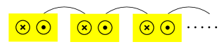
Figure 2: (Color online) Pictorial representation for the selected backscattering in the symmetry class D. Each yellow box represents a quantum wire composed of two Majorana degrees of freedom. The wires are enumerated by $I=1,\cdots,N$ in ascending order from left to right. For any $I$, the Majorana modes are denoted by $\chi^{\,}_{\mathrm{R},I}$ and $\chi^{\,}_{\mathrm{L},I}$ reading from left to right, respectively.

II.4 The ten-fold way via non-Abelian bosonization

The goal of this section is to derive the tenfold way in two-dimensional space by modeling two-dimensional space as an array of wires on which noninteracting degrees of freedom (i) obey the Majorana algebra, (ii) propagate freely along any wire, (iii) while they can hop between consecutive wires. The novelty in deriving the tenfold way is that we shall use non-Abelian bosonization techniques, and apply the singular value decomposition on the mass matrix, as described above, to count the number of gapless edge modes.

We shall consider the symmetry classes D and DIII that, together with the symmetry classes C, A, and AII, correspond to the topological superconductors and insulators in two-dimensional space from the tenfold way.  Schnyder et al. (2009); Kitaev (2009); Schnyder et al. (2008); Ryu et al. (2010) The symmetry classes C, A, and AII are treated in Appendix B.

II.4.1 The symmetry class D

We shall use a path integral representation of the array of quantum wires. There will be $2MN$ independent Grassmann variables $\chi^{\,}_{\alpha,\mathrm{f},I}$, where $\alpha=\mathrm{R},\mathrm{L}$ distinguish a right- from a left-mover, $\mathrm{f}=1,\cdots,M$ is a flavor index, and $I=1,\cdots,N$ enumerates the wire.

The simplest model for an array of quantum wires in the symmetry class D to realize a topological gapped phase assumes

$$M=1,\qquad\chi^{\,}_{\alpha,I}(t,x),$$ (41a)

for $$\alpha=\mathrm{R},\mathrm{L} I=1,\cdots,N I=1\,\cdots\,N$$ and . We have thus assigned a pair of Majorana fermions to each wire . We define the action

$$S^{(\mathrm{D})}_{0}:=\int\mathrm{d}t\int\mathrm{d}x\,\mathcal{L}^{(\mathrm{D})}_{0}$$ (41b)

with

$$\mathcal{L}^{(\mathrm{D})}_{0}:=\frac{\mathrm{i}}{2}\sum_{I=1}^{N}\Bigl{[}\chi^{\,}_{\mathrm{R},I}(\partial^{\,}_{t}+\partial^{\,}_{x})\chi^{\,}_{\mathrm{R},I}+\chi^{\,}_{\mathrm{L},I}(\partial^{\,}_{t}-\partial^{\,}_{x})\chi^{\,}_{\mathrm{L},I}\Bigr{]}.$$ (41c)

We also define the Grassmann partition function

$$Z^{(\mathrm{D})}_{0}:=\int\mathcal{D}[\chi]\,e^{+\mathrm{i}S^{(\mathrm{D})}_{0}}.$$ (41d)

The theory with the partition function $Z^{(\mathrm{D})}_{0}$ is critical, for there are $2N$ decoupled massless Majorana modes that are dispersing in $(1+1)$-dimensional Minkowski space and time. Hence, the central charge $c^{(\mathrm{D})}_{0}$ for the partition function $Z^{(\mathrm{D})}_{0}$ is

$$c^{(\mathrm{D})}_{0}=\frac{N}{2}.$$ (42a)

The partition function $$Z^{(\mathrm{D})}_{0} (O^{(\mathrm{R})},O^{(\mathrm{L})})\in O^{\,}_{\mathrm{R}}(N)\times O^{\,}_{\mathrm{L}}(N)$$ is invariant under any local linear transformation defined by the fundamental rule

$$\begin{split}&\chi^{\,}_{\mathrm{R}}(t-x)\mapsto O^{(\mathrm{R})}(t-x)\,\chi^{\,}_{\mathrm{R}}(t-x),\\ &\chi^{\,}_{\mathrm{L}}(t+x)\mapsto O^{(\mathrm{L})}(t+x)\,\chi^{\,}_{\mathrm{L}}(t+x).\end{split}$$ (42b)

The partition function $$Z^{(\mathrm{D})}_{0}$$ is also invariant under the antilinear transformation with the fundamental rule

$$\begin{split}&\chi^{\,}_{\mathrm{R}}(t,x)\mapsto\chi^{\,}_{\mathrm{L}}(-t,x),\quad\chi^{\,}_{\mathrm{L}}(t,x)\mapsto\chi^{\,}_{\mathrm{R}}(-t,x),\end{split}$$ (42c)

that implements reversal of time in such a way that it squares to the identity (see Appendix A). Even though reversal of time (42c) is a symmetry of the partition function $Z^{(\mathrm{D})}_{0}$, we shall not impose invariance under reversal of time (42c) for a generic representative of the symmetry class D.

Any partition function $Z^{(\mathrm{D})}$ for the array of quantum wires is said to belong to the symmetry class D if $Z^{(\mathrm{D})}$ is invariant under the linear transformation (fermion parity) with the fundamental rule

$$\chi^{\,}_{\alpha}\mapsto-\chi^{\,}_{\alpha},$$ (43)

for $\alpha=\mathrm{R},\mathrm{L}$.

We seek a local single-particle perturbation $\mathcal{L}^{(\mathrm{D})}_{\mathrm{mass}}$ that satisfies three conditions when added to the Lagrangian density (41c).

Condition D.1 It must be invariant under the transformation (43).

Condition D.2 It must gap completely the theory with the partition function $Z^{(\mathrm{D})}_{0}$ if we impose the periodic boundary conditions

$$\chi^{\,}_{\alpha,I}(t,x)=\chi^{\,}_{\alpha,I+N}(t,x),$$ (44)

for $\alpha=\mathrm{R},\mathrm{L}$ and $I=1,\cdots,N$.

Condition D.3 The partition function $Z^{(\mathrm{D})}$ with the Lagrangian density $\mathcal{L}^{(\mathrm{D})}_{0}+\mathcal{L}^{(\mathrm{D})}_{\mathrm{mass}}$ must be a theory with the central charge

$$c^{(\mathrm{D})}=\frac{1}{2}$$ (45)

if open boundary condition are imposed.

Conditions D.1, D.2, and D.3 imply that we may assign wire $I=1$ the left-chiral central charge $1/2$ and wire $I=N$ the right-chiral central charge $1/2$. For example, if wire $I=1$ supports a right-moving (i.e., chiral) Majorana edge mode, then wire $I=N$ supports a left-moving (i.e., chiral) Majorana edge mode.

We make the Ansatz

$$\mathcal{L}^{(\mathrm{D})}_{\mathrm{mass}}:=\mathrm{i}\lambda\,\sum_{I=1}^{N-1}\chi^{\,}_{\mathrm{L},I}\,\chi^{\,}_{\mathrm{R},I+1}$$ (46)

with $\lambda$ a real-valued coupling. To establish that the Ansatz (46) meets Conditions D.2 and D.3, we use non-Abelian bosonization. We choose the non-Abelian bosonization scheme by which the partition function is given by the path integral

$$Z^{(\mathrm{D})}=\int\mathcal{D}[G]\,e^{\mathrm{i}S^{(\mathrm{D})}}.$$ (47a)

The field $$G\in O(N) \mathcal{D}[G] O(N) S^{(\mathrm{D})} S^{(\mathrm{D})}_{0} S^{(\mathrm{D})}_{\mathrm{mass}} S^{(\mathrm{D})}_{0}$$ is a matrix of bosons. The measure is constructed from the Haar measure on . The action is the sum of the actions and . The action is

$$\begin{split}S^{(\mathrm{D})}_{0}=&\,\frac{1}{16\pi}\int\mathrm{d}t\int\mathrm{d}x\,\mathrm{tr}\,\left(\partial^{\,}_{\mu}G\,\partial^{\mu}G^{-1}\right)\\ &\,+\frac{1}{24\pi}\int\limits_{B}\mathrm{d}^{3}y\,\mathcal{L}^{(\mathrm{D})}_{\mathrm{WZW}},\end{split}$$ (47b)

where

$$\mathcal{L}^{(\mathrm{D})}_{\mathrm{WZW}}=\epsilon^{ijk}\,\mathrm{tr}\,\Bigl{[}(\bar{G}^{-1}\partial^{\,}_{i}\bar{G})\,(\bar{G}^{-1}\partial^{\,}_{j}\bar{G})(\bar{G}^{-1}\partial^{\,}_{k}\bar{G})\Bigr{]}.$$ (47c)

The action $$S^{(\mathrm{D})}_{\mathrm{mass}}$$ stems from the Lagrangian density

$$\mathcal{L}^{(\mathrm{D})}_{\mathrm{mass}}=\lambda\,\sum_{I=1}^{N-1}G^{\,}_{I,I+1}\equiv\,\lambda\,\mathrm{tr}\left(M^{(\mathrm{D})}\,G\right).$$ (47d)

The second equality is established by using the non-Abelian bosonization formula (30) (we have set the mass parameter $$m^{\,}_{\mathrm{uv}}=1 N\times N M^{(\mathrm{D})}$$). The matrix is represented by

$$M^{(\mathrm{D})}:=\begin{pmatrix}0&0&0&0&0&0&\cdots\\ 1&0&0&0&0&0&\cdots\\ 0&1&0&0&0&0&\cdots\\ 0&0&1&0&0&0&\cdots\\ 0&0&0&1&0&0&\cdots\\ 0&0&0&0&1&0&\cdots\\ \vdots&\vdots&\vdots&\vdots&\vdots&\vdots&\ddots\\ \end{pmatrix}.$$ (47e)

The singular value decomposition of the mass matrix (47e) gives

$$M^{(\mathrm{D})}_{\mathrm{diag}}=\mathrm{diag}\left(\underbrace{\Omega^{\,}_{1},\Omega^{\,}_{2},\Omega^{\,}_{3},...,\Omega^{\,}_{N-1}}^{\,}_{N-1},0\right).$$ (48)

The quadratic perturbation (47d) thus reduces the central charge $c^{(\mathrm{D})}_{0}=N/2$ by the amount $(N-1)/2$, i.e., the central charge for the theory with the partition function $Z^{(\mathrm{D})}$ is

$$c^{(\mathrm{D})}=\frac{N}{2}-\frac{N-1}{2}=\frac{1}{2}.$$ (49)

We have constructed a topological superconductor with the gapless chiral Majorana mode $\chi^{\,}_{\mathrm{R},I=1}$ propagating along edge $I=1$ (the left eigenstate of the mass matrix) vand the gapless chiral Majorana mode of opposite chirality $\chi^{\,}_{\mathrm{L},I=N}$ propagating along edge $I=N$ (the right eigenstate of the mass matrix). This construction is summarized by Fig. 2.

The symmetry class D has the $\mathbb{Z}$ topological classification for the following reason. If one takes an arbitrary integer number $\nu$ of copies of the gapless edge theory, these $\nu$-copies remain gapless. The stability of the $\nu$ chiral gapless edge modes within either wire 1 or wire $N$ is guaranteed because backscattering among these gapless chiral edges modes is not allowed kinematically.

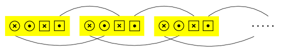
Figure 3: (Color online) Pictorial representation for the selected backscattering in the symmetry class DIII. Each yellow box represents a quantum wire composed of four-Majorana degrees of freedom. The wires are enumerated by $I=1,\cdots,N$ in ascending order from left to right. For any $I$, the Majorana modes are denoted by $\chi^{\,}_{\mathrm{R},+,I}$, $\chi^{\,}_{\mathrm{L},+,I}$, $\chi^{\,}_{\mathrm{R},-,I}$, and $\chi^{\,}_{\mathrm{L},-,I}$ reading from left to right, respectively.

II.4.2 The symmetry class DIII

The simplest model for an array of quantum wires in the symmetry class DIII to realize a topological gapped phase assumes

$$M=2,\quad\chi^{\,}_{\alpha,\mathrm{f},I}(t,x),$$ (50a)

for $$\alpha=\mathrm{R},\mathrm{L} \mathrm{f}=\pm I=1,\cdots,N I=1\,\cdots\,N$$, , and . We have thus assigned four Majorana fermions to each wire . We define the action

$$S^{(\mathrm{DIII})}_{0}:=\int\mathrm{d}t\int\mathrm{d}x\,\mathcal{L}^{(\mathrm{DIII})}_{0}$$ (50b)

with

$$\begin{split}\mathcal{L}^{(\mathrm{DIII})}_{0}:=&\,\frac{\mathrm{i}}{2}\sum_{I=1}^{N}\sum_{\sigma=\pm}\Bigl{[}\chi^{\,}_{\mathrm{R},\sigma,I}\left(\partial^{\,}_{t}+\partial^{\,}_{x}\right)\chi^{\,}_{\mathrm{R},\sigma,I}\\ &\,+\chi^{\,}_{\mathrm{L},\sigma,I}\left(\partial^{\,}_{t}-\partial^{\,}_{x}\right)\chi^{\,}_{\mathrm{L},\sigma,I}\Bigr{]}.\end{split}$$ (50c)

We also define the Grassmann partition function

$$Z^{(\mathrm{DIII})}_{0}:=\int\mathcal{D}[\chi]\,e^{\mathrm{i}S^{(\mathrm{DIII})}_{0}}.$$ (50d)

The theory with the partition function $Z^{(\mathrm{DIII})}_{0}$ is critical, for there are $4N$ decoupled massless Majorana modes that are dispersing in $(1+1)$-dimensional Minkowski space and time. Hence, the central charge for the theory with the partition function $Z^{(\mathrm{DIII})}_{0}$ is

$$c^{(\mathrm{DIII})}_{0}=N.$$ (51a)

The partition function $$Z^{(\mathrm{DIII})}_{0} (O^{(\mathrm{R})},O^{(\mathrm{L})})\in O^{\,}_{\mathrm{R}}(2N)\times O^{\,}_{\mathrm{L}}(2N)$$ is invariant under any local transformation defined by

$$\begin{split}&\chi^{\,}_{\mathrm{R}}(t-x)\mapsto O^{(\mathrm{R})}(t-x)\,\chi^{\,}_{\mathrm{R}}(t-x),\\ &\chi^{\,}_{\mathrm{L}}(t+x)\mapsto O^{(\mathrm{L})}(t+x)\,\chi^{\,}_{\mathrm{L}}(t+x).\end{split}$$ (51b)

It is also invariant under the antilinear transformation with the fundamental rules

$$\begin{split}&\chi^{\,}_{\mathrm{R},+,I}(t,x)\mapsto+\chi^{\,}_{\mathrm{L},-,I}(-t,x),\\ &\chi^{\,}_{\mathrm{R},-,I}(t,x)\mapsto-\chi^{\,}_{\mathrm{L},+,I}(-t,x),\\ &\chi^{\,}_{\mathrm{L},+,I}(t,x)\mapsto+\chi^{\,}_{\mathrm{R},-,I}(-t,x),\\ &\chi^{\,}_{\mathrm{L},-,I}(t,x)\mapsto-\chi^{\,}_{\mathrm{R},+,I}(-t,x),\end{split}$$ (51c)

that implements reversal of time in such a way that reversal of time squares to minus the identity (see Appendix A).

Any partition function $Z^{(\mathrm{DIII})}$ for the array of quantum wires is said to belong to the symmetry class DIII if reversal of time is a symmetry represented by an antilinear and involutive operation that squares to minus the identity, i.e., Eq. (51c), and if $Z^{(\mathrm{DIII})}$ is invariant under the linear transformation (fermion parity) with the fundamental rule

$$\chi^{\,}_{\alpha,\mathrm{f},I}\mapsto-\chi^{\,}_{\alpha,\mathrm{f},I},$$ (52)

for $\alpha=\mathrm{R},\mathrm{L}$, $\mathrm{f}=\pm$, and $I=1,\cdots,N$.

We seek a local single-particle perturbation $\mathcal{L}^{(\mathrm{DIII})}_{\mathrm{mass}}$ that satisfies three conditions when added to the Lagrangian density (50c).

Condition DIII.1 It must be invariant under the transformations (51c) and (52).

Condition DIII.2 It must gap completely the theory with the partition function $Z^{(\mathrm{DIII})}_{0}$ if we impose the periodic boundary conditions

$$\chi^{\,}_{\alpha,\mathrm{f},I}(t,x)=\chi^{\,}_{\alpha,\mathrm{f},I+N}(t,x)$$ (53)

for $\alpha=\mathrm{R},\mathrm{L}$, $\mathrm{f}=\pm$, and $I=1,\cdots,N$.

Condition DIII.3 The partition function $Z^{(\mathrm{DIII})}$ with the Lagrangian density $\mathcal{L}^{(\mathrm{DIII})}_{0}+\mathcal{L}^{(\mathrm{DIII})}_{\mathrm{mass}}$ must be a theory with the central charge

$$c^{(\mathrm{DIII})}=1$$ (54)

if open boundary condition are imposed.

Conditions DIII.1, DIII.2, and DIII.3 imply that we may assign wire $I=1$ the central charge $1/2$ and wire $I=N$ the central charge $1/2$, for wires $I=1$ and $I=N$ both support a Kramers degenerate pair of right- and left-moving Majorana edge modes.

We make the Ansatz

$$\mathcal{L}^{(\mathrm{DIII})}_{\mathrm{mass}}:=\sum_{I=1}^{N-1}\mathrm{i}\lambda\,\left(\chi^{\,}_{\mathrm{L},-,I}\,\chi^{\,}_{\mathrm{R},-,I+1}-\chi^{\,}_{\mathrm{R},+,I}\,\chi^{\,}_{\mathrm{L},+,I+1}\right)$$ (55)

with $\lambda$ a real-valued coupling. Condition DIII.1 is met by construction. To establish that the Ansatz (55) meets Conditions DIII.2 and DIII.3, we use non-Abelian bosonization. We choose the non-Abelian bosonization scheme by which the partition function is given by the path integral

$$Z^{(\mathrm{DIII})}=\int\mathcal{D}[G]\,e^{\mathrm{i}S^{(\mathrm{DIII})}}.$$ (56a)

The field $$G\in O(2N) \mathcal{D}[G] O(2N) S^{(\mathrm{DIII})} S^{(\mathrm{DIII})}_{0} S^{(\mathrm{DIII})}_{\mathrm{mass}} S^{(\mathrm{DIII})}_{0}$$ is a matrix of bosons. The measure is constructed from the Haar measure on . The action is the sum of the actions and . The action is

$$\begin{split}S^{(\mathrm{DIII})}_{0}=&\,\frac{1}{16\pi}\int\mathrm{d}t\int\mathrm{d}x\,\mathrm{tr}\,\left(\partial^{\,}_{\mu}G\,\partial^{\mu}G^{-1}\right)\\ &\,+\frac{1}{24\pi}\int\limits_{B}\mathrm{d}^{3}y\,\mathcal{L}^{(\mathrm{DIII})}_{\mathrm{WZW}},\end{split}$$ (56b)

where

$$\mathcal{L}^{(\mathrm{DIII})}_{\mathrm{WZW}}=\epsilon^{ijk}\,\mathrm{tr}\,\Bigl{[}(\bar{G}^{-1}\partial^{\,}_{i}\bar{G})\,(\bar{G}^{-1}\partial^{\,}_{j}\bar{G})(\bar{G}^{-1}\partial^{\,}_{k}\bar{G})\Bigr{]}.$$ (56c)

The action $$S^{(\mathrm{DIII})}_{\mathrm{mass}}$$ stems from the Lagrangian density

$$\begin{split}\mathcal{L}^{(\mathrm{DIII})}_{\mathrm{mass}}=&\,\sum_{I=1}^{N-1}\lambda\,\left(G^{\,}_{(-,I),(-,I+1)}+G^{\,}_{(+,I+1),(+,I)}\right)\\ \equiv&\,\lambda\,\mathrm{tr}\,\left(M^{(\mathrm{DIII})}\,G\right).\end{split}$$ (56d)

The second equality is established by using the non-Abelian bosonization formula (30) (we have set the mass parameter $$m^{\,}_{\mathrm{uv}}=1 2N\times 2N M^{(\mathrm{DIII})}$$). The matrix is represented by

$$M^{(\mathrm{DIII})}:=\begin{pmatrix}0&B&0&0&0&0&\cdots\\ B^{\mathsf{T}}&0&B&0&0&0&\cdots\\ 0&B^{\mathsf{T}}&0&B&0&0&\cdots\\ 0&0&B^{\mathsf{T}}&0&B&0&\cdots\\ 0&0&0&B^{\mathsf{T}}&0&B&\cdots\\ 0&0&0&0&B^{\mathsf{T}}&0&\cdots\\ \vdots&\vdots&\vdots&\vdots&\vdots&\vdots&\ddots\\ \end{pmatrix}$$ (56e)

in the basis for which $$B 2\times 2$$ is the matrix

$$B:=\begin{pmatrix}\overbrace{0}^{(-,+)}&\overbrace{0}^{(-,-)}\\ \underbrace{1}_{(+,+)}&\underbrace{0}_{(+,-)}\end{pmatrix}.$$ (56f)

For any $N>0$, the $2N\times 2N$ matrices $M^{(\mathrm{DIII})}$ defined by (56e) has two vanishing and $2\times(N-1)$ nonvanishing eigenvalues.

The quadratic perturbation (56d) thus reduces the central charge $c^{(\mathrm{DIII})}_{0}=2\times N/2$ by the amount $2\times(N-1)/2$, i.e., the central charge for the theory with the partition function $Z^{(\mathrm{DIII})}$ is

$$c^{(\mathrm{DIII})}=\frac{2\times N}{2}-\frac{2\times(N-1)}{2}=1.$$ (57)

We have constructed a topological superconductor with the gapless pair of helical Majorana modes $(\chi^{\,}_{\mathrm{L},+,I},\chi^{\,}_{\mathrm{R},-,I})^{\,}_{I=1}$ propagating along edge $I=1$ and the gapless pair of helical Majorana modes $(\chi^{\,}_{\mathrm{R},+,I},\chi^{\,}_{\mathrm{L},-,I})^{\,}_{I=N}$ propagating along edge $I=N$. This construction is summarized by Fig. 3.

The symmetry class DIII has the $\mathbb{Z}^{\,}_{2}$ classification from the following argument. We take $\nu$ copies of the gapless edge theories on the right edge ($I=N$). We drop the index $I=N$ for notational simplicity. The most general backscattering processes are encoded by

$$\mathcal{L}^{(\mathrm{DIII})}_{N}:=\sum_{a,b=1}^{\nu}\mathrm{i}\chi^{\,}_{\mathrm{L},-,a}\,\lambda^{\,}_{ab}\,\chi^{\,}_{\mathrm{R},+,b}.$$ (58)

Hermiticity dictates here that

$$\lambda^{\,}_{ab}=\lambda^{*}_{ab},\qquad a,b=1,\cdots,\nu,$$ (59)

i.e., all matrix elements $\lambda^{\,}_{ab}$ are real valued. Time-reversal symmetry dictates that

$$\sum_{a,b=1}^{\nu}\mathrm{i}\chi^{\,}_{\mathrm{L},-,a}\,\lambda^{\,}_{ab}\,\chi^{\,}_{\mathrm{R},+,b} \mapsto \sum_{a,b=1}^{\nu}(-\mathrm{i})(-1)\chi^{\,}_{\mathrm{R},+,a}\,\lambda^{\,}_{ab}\,\chi^{\,}_{\mathrm{L},-,b}$$

$$= \sum_{a,b=1}^{\nu}\mathrm{i}\chi^{\,}_{\mathrm{R},+,a}\,\lambda^{\,}_{ab}\,\chi^{\,}_{\mathrm{L},-,b}$$

$$= \sum_{a,b=1}^{\nu}\mathrm{i}\chi^{\,}_{\mathrm{R},+,b}\,\lambda^{\,}_{ba}\chi^{\,}_{\mathrm{L},-,a}$$

$$= \sum_{a,b=1}^{\nu}\mathrm{i}\chi^{\,}_{\mathrm{L},-,a}\,(-\lambda^{\,}_{ba})\,\chi^{\,}_{\mathrm{R},+,b},$$

i.e., the real-valued matrix elements (59) must also be antisymmetric

$$\lambda^{\,}_{ab}=-\lambda^{\,}_{ba},\qquad a,b=1,\cdots,\nu.$$ (60b)

Because of the identity

$$\mathrm{det}\,(\lambda^{\,}_{ab})=\mathrm{det}\,(\lambda^{\,}_{ab})^{\mathsf{T}}=\mathrm{det}\,(-\lambda^{\,}_{ab})=(-1)^{\nu}\,\mathrm{det}\,(\lambda^{\,}_{ab}),$$ (61)

if follows that the matrix $(\lambda^{\,}_{ab})$ has at least one vanishing eigenvalue when $\nu$ is odd. When $\nu$ is odd, a pair of helical edge modes must remain gapless. When $\nu$ is even, all pairs of helical edge modes can be gapped. The topological classification $\mathbb{Z}^{\,}_{2}$ for the symmetry class DIII in 2D follows.

III Non-Abelian topological order out of coupled wires

We have shown in Sec. II.4 (plus Appendix B) that the tenfold way in two-dimensional space can be derived from a one-dimensional array of quantum wires, whereby each wire hosts Majorana fermions (i.e., “real-valued” fermions) that may hop between consecutive wires through one-body backscattering. This derivation of the tenfold way in two-dimensional space presumes no more and no less than the existence of noninteracting Majorana fermions.

In each of the superconducting symmetry classes D, DIII, and C, the existence of the numbers 2, 4, and 4 of noninteracting Majorana fermions per wire, respectively, was shown to be sufficient to realize a superconducting ground state with protected edge states. The numbers 2, 4, and 4 are the same numbers of complex fermions per wire used in Ref. Neupert et al., 2014 to stabilize short-ranged entangled topological superconducting ground states in the symmetry classes D, DIII, and C for chains of wires that were coupled through strictly many-body interactions. The derivation of the tenfold way in Sec. II.4 (plus Appendix B) is thus more economical than that in Ref. Neupert et al., 2014. In fact, the numbers of Majorana fermions per wire that we have postulated in Sec. II.4 and in Appendix B are the minimum numbers of Majorana fermions per wire required to realize short-ranged entangled gapped phases supporting protected edge states in the tenfold way.

There is a drawback to this derivation, however. Majorana fermions are not the fundamental fermions in condensed matter physics. The electron is. Majorana fermions only emerge as quasiparticles out of interactions that electrons undergo with themselves or with collective modes such as phonons or spin waves. One plain way to state the drawback of the derivation in Sec. II.4 is that it takes as the starting point an already fractionalized electron.

In this section, we are going to modify our strategy as follows. Each wire in the one-dimensional array of wires supports electrons instead of Majorana fermions. Second, any interaction that gaps the bulk will be built out of one-body or many-body electron-electron interactions obeying two conditions. First, interactions explicitly conserve the electron number. Second, the spatial range of all interactions are bounded from above by one finite length scale. In this way, the interaction conserves the total electron number and are local. Nevertheless, we shall insist on recovering Majorana fermions or their generalizations (parafermions) on the boundaries by properly choosing the many-body electron-electron interactions.

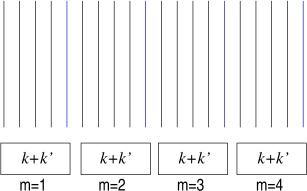
Figure 4: (Color online) Chain of $N$ wires grouped into $n$ bundles of $k+k^{\prime}$ wires with $N=20$, $n=4$, $k=4$ and $k^{\prime}=1$. The chain of wires is labeled by $I=1,\cdots,N$. The bundles of $k+k^{\prime}$ wires are labeled by the teletype font $\texttt{m}=1,\cdots,n$.

III.1 One-dimensional arrays of quantum wires with local current-current interactions

A chain of $N$ decoupled wires is labeled with the index $I=1,\cdots,N$. Electrons move freely along any one of these $N$ wires. Their spin-1/2 projections along the quantization axis are $\sigma=\uparrow,\downarrow$. For simplicity, all wires are identical. At low energies, we postulate the noninteracting Lagrangian density  

$$\begin{split}\mathcal{L}^{\,}_{0}:=&\,\mathrm{i}\sum_{I=1}^{N}\sum_{\sigma=\uparrow,\downarrow}\Big{[}\psi^{*}_{\mathrm{R},\sigma,I}\,(\partial^{\,}_{t}+\partial^{\,}_{x})\,\psi^{\,}_{\mathrm{R},\sigma,I}\\ &\,+\psi^{*}_{\mathrm{L},\sigma,I}\,(\partial^{\,}_{t}-\partial^{\,}_{x})\,\psi^{\,}_{\mathrm{L},\sigma,I}\Big{]}\end{split}$$ (62a)

with the action

$$S^{\,}_{0}:=\int\mathrm{d}t\int\mathrm{d}x\,\mathcal{L}^{\,}_{0}$$ (62b)

and the partition function

$$Z^{\,}_{0}:=\int\mathcal{D}[\psi^{*},\psi]\ e^{\mathrm{i}S^{\,}_{0}}.$$ (62c)

The partition function $Z^{\,}_{0}$ is invariant under any local linear transformation

$$(U^{(\mathrm{R})},U^{(\mathrm{L})})\in U^{\,}_{\mathrm{R}}(2N)\times U^{\,}_{\mathrm{L}}(2N)$$ (63a)

defined by the fundamental rules

$$\begin{split}&\psi^{*\mathsf{T}}_{\mathrm{R}}(t-x)\mapsto\psi^{*\mathsf{T}}_{\mathrm{R}}(t-x)\,U^{(\mathrm{R}){\dagger}}(t-x),\\ &\psi^{*\mathsf{T}}_{\mathrm{L}}(t+x)\mapsto\psi^{*\mathsf{T}}_{\mathrm{L}}(t+x)\,U^{(\mathrm{L}){\dagger}}(t+x),\end{split}$$ (63b)

and

$$\begin{split}&\psi^{\,}_{\mathrm{R}}(t-x)\mapsto U^{(\mathrm{R})}(t-x)\,\psi^{\,}_{\mathrm{R}}(t-x),\\ &\psi^{\,}_{\mathrm{L}}(t+x)\mapsto U^{(\mathrm{L})}(t+x)\,\psi^{\,}_{\mathrm{L}}(t+x),\end{split}$$ (63c)

on the Grassmann integration variables. The corresponding central charge is

$$c^{\,}_{0}=2N.$$ (64)

The partition function $Z^{\,}_{0}$ is also invariant under reversal of time, whereby this operation is represented by the antilinear transformation with the fundamental rules

$$\psi^{*}_{\mathrm{R},\uparrow,I}\mapsto+\psi^{*}_{\mathrm{L},\downarrow,I},\qquad\psi^{*}_{\mathrm{R},\downarrow,I}\mapsto-\psi^{*}_{\mathrm{L},\uparrow,I},$$ (65a)

$$\psi^{*}_{\mathrm{L},\uparrow,I}\mapsto+\psi^{*}_{\mathrm{R},\downarrow,I},\qquad\psi^{*}_{\mathrm{L},\downarrow,I}\mapsto-\psi^{*}_{\mathrm{R},\uparrow,I},$$ (65b)

and

$$\psi^{\,}_{\mathrm{R},\uparrow,I}\mapsto+\psi^{\,}_{\mathrm{L},\downarrow,I},\qquad\psi^{\,}_{\mathrm{R},\downarrow,I}\mapsto-\psi^{\,}_{\mathrm{L},\uparrow,I},$$ (65c)

$$\psi^{\,}_{\mathrm{L},\uparrow,I}\mapsto+\psi^{\,}_{\mathrm{R},\downarrow,I},\qquad\psi^{\,}_{\mathrm{L},\downarrow,I}\mapsto-\psi^{\,}_{\mathrm{R},\uparrow,I},$$ (65d)

on the Grassmann integration variables.

The chain-resolved symmetry $U^{\,}_{\mathrm{R}}(2)\times U^{\,}_{\mathrm{L}}(2)$, a subgroup of the symmetry group (63a), is broken by coupling consecutive chains through one-body tunnelings.

Example 1. The uniform one-body hopping of the electrons between consecutive chains

$$\begin{split}\mathcal{L}^{\,}_{\mathrm{FS}}:=-t\sum_{I=1}^{N}\left[\psi^{*\mathsf{T}}_{\mathrm{R},I}\,\psi^{\,}_{\mathrm{R},I+1}+\psi^{*\mathsf{T}}_{\mathrm{R},I+1}\,\psi^{\,}_{\mathrm{R},I}+(\mathrm{R}\to\mathrm{L})\right],\end{split}$$ (66)

where $t$ is positive and periodic boundary conditions by which $I\equiv I+N$ are imposed on the Grassmann fields, turns the one-dimensional critical theory (62) into an anisotropic two-dimensional gas of electrons in the thermodynamic limit $N\to\infty$.

Example 2. The staggered one-body hopping

$$\begin{split}\mathcal{L}^{\,}_{\mathrm{D}}:=&\,-\mathrm{i}t\sum_{I=1}^{N}\Bigl{[}\psi^{*\mathsf{T}}_{\mathrm{R},I}\,\psi^{\,}_{\mathrm{L},I+1}-\psi^{*\mathsf{T}}_{\mathrm{L},I+1}\,\psi^{\,}_{\mathrm{R},I}\\ &\,+\psi^{*\mathsf{T}}_{\mathrm{L},I}\,\psi^{\,}_{\mathrm{R},I+1}-\psi^{*\mathsf{T}}_{\mathrm{R},I+1}\,\psi^{\,}_{\mathrm{L},I}\Bigr{]},\end{split}$$ (67)

where $t$ is positive and periodic boundary conditions by which $I\equiv I+N$ are imposed on the Grassmann fields, turns the one-dimensional critical theory (62) into an anisotropic two-dimensional Dirac gas of electrons in the thermodynamic limit $N\to\infty$, i.e., a quasi-one-dimensional representation of graphene.

Coupling the chains through many-body tunnelings that preserve the chain-resolved $U^{\,}_{\mathrm{R}}(2)\times U^{\,}_{\mathrm{L}}(2)$ subgroup of the symmetry group (63a) (i.e., the independent conservation of the right- and left-moving electronic charge and spin in each wire) also delivers two-dimensional gapless phases of matter in the thermodynamic limit $N\to\infty$.   O’Hern et al. (1999); Emery et al. (2000); Vishwanath and Carpentier (2001); Mukhopadhyay et al. (2001)

Example 3. The four-fermion interactions

$$\mathcal{L}^{\,}_{\mathrm{SLL}}:=\sum_{I,J=1}^{N}\left[\left(\psi^{*\mathsf{T}}_{\mathrm{R},I}\,\psi^{\,}_{\mathrm{R},I}\right)V^{\,}_{IJ}\,\left(\psi^{*\mathsf{T}}_{\mathrm{R},J}\,\psi^{\,}_{\mathrm{R},J}\right)+\left(\mathrm{R}\to\mathrm{L}\right)\right]$$ (68)

with $V^{\,}_{IJ}=V^{\,}_{JI}$ a symmetric and real-valued $N\times N$ matrix and periodic boundary conditions by which $I\equiv I+N$ are imposed on the Grassmann fields, stabilize a sliding Luttinger liquid (SLL) phase in the thermodynamic limit $N\to\infty$, whose defining properties is that of algebraic order along the quantum wires in contrast to exponentially decaying correlation functions in the direction transverse to that of the quantum wires.   O’Hern et al. (1999); Emery et al. (2000); Vishwanath and Carpentier (2001); Mukhopadhyay et al. (2001)

We are after two-dimensional phases that are insulating when periodic boundary conditions hold. This can always be achieved by a suitable combination of a breaking of translation symmetry, on the one hand, and of an interaction between left- and right-movers, on the other hand. For this reason, we shall ignore couplings of the quantum wires that deliver gapless two-dimensional phases as in Examples 1, 2, and 3 relative to those couplings between left- and right-movers responsible for an insulating phase when periodic boundary conditions hold.

This section is organized as follows. We begin by showing in Sec. III.2 how to combine one-body and current-current interactions that fully gap the critical theory (62). We proceed in Sec. III.3 by coupling the wires through current-current interactions so that (i) time-reversal symmetry is explicitly broken, (ii) the critical theory (62) is fully gapped when periodic boundary conditions are imposed along the chain of quantum wires, and (iii) there remains gapless edge states that realize chiral conformal field theories with the chiral central charge

$$0<c<3$$ (69)

on any one of the two boundaries close to wire $1$ and $N$, respectively, when open boundary conditions are imposed along the chain of quantum wires. We close with Sec. III.4 by selecting interactions that are time-reversal symmetric.

III.2 Complete gapping

As a warm up, we observe that the symmetry group (63a) contains as a subgroup the symmetry group $\Big{(}U^{\,}_{\mathrm{R}}(2)\times U^{\,}_{\mathrm{L}}(2)\Big{)}\times\cdots\times\Big{(}U^{\,}_{\mathrm{R}}(2)\times U^{\,}_{\mathrm{L}}(2)\Big{)}$. We are assigning to the unitary group $U(2)$ of $2\times 2$ matrices the label R and L when it acts on the right- and left-moving electrons, respectively, from a given wire. The partition function $Z^{\,}_{0}$ is, indeed, invariant under any local linear transformation

$$\Big{(}U^{(\mathrm{R})}_{I},U^{(\mathrm{L})}_{I}\Big{)}\in U^{\,}_{\mathrm{R}}(2)\times U^{\,}_{\mathrm{L}}(2)$$ (70a)

defined by the fundamental rules

$$\begin{split}&\psi^{*}_{\mathrm{R},\sigma,I}(t-x)\mapsto\psi^{*}_{\mathrm{R},\sigma^{\prime},I}(t-x)\,\left(U^{(\mathrm{R}){\dagger}}_{I}\right)^{\,}_{\sigma^{\prime}\sigma}(t-x),\\ &\psi^{*}_{\mathrm{L},\sigma,I}(t+x)\mapsto\psi^{*}_{\mathrm{L},\sigma^{\prime},I}(t+x)\,\left(U^{(\mathrm{L}){\dagger}}_{I}\right)^{\,}_{\sigma^{\prime}\sigma}(t+x),\end{split}$$ (70b)

and

$$\begin{split}&\psi^{\,}_{\mathrm{R},\sigma,I}(t-x)\mapsto\left(U^{(\mathrm{R})}_{I}\right)^{\,}_{\sigma\sigma^{\prime}}(t-x)\,\psi^{\,}_{\mathrm{R},\sigma^{\prime},I}(t-x),\\ &\psi^{\,}_{\mathrm{L},\sigma,I}(t+x)\mapsto\left(U^{(\mathrm{L})}_{I}\right)^{\,}_{\sigma\sigma^{\prime}}(t+x)\,\psi^{\,}_{\mathrm{L},\sigma^{\prime},I}(t+x),\end{split}$$ (70c)

for any $\sigma=\uparrow,\downarrow$ and any $I=1,\cdots,N$ on the Grassmann integration variables. These symmetries imply for the light-cone components [we choose the multiplicative normalization from Ref. Affleck, 1990; Affleck and Ludwig, 1991a, b rather than the one in Eq. (22)]

$$T^{\,}_{\mathrm{R},I}:=\frac{\mathrm{i}}{2\pi}\sum_{\sigma=\uparrow,\downarrow}\psi^{*}_{\mathrm{R},\sigma,I}\,\left(\partial^{\,}_{t}-\partial^{\,}_{x}\right)\,\psi^{\,}_{\mathrm{R},\sigma,I}$$ (71a)

and

$$T^{\,}_{\mathrm{L},I}:=\frac{\mathrm{i}}{2\pi}\sum_{\sigma=\uparrow,\downarrow}\psi^{*}_{\mathrm{L},\sigma,I}\,\left(\partial^{\,}_{t}+\partial^{\,}_{x}\right)\,\psi^{\,}_{\mathrm{L},\sigma,I}$$ (71b)

of the energy-momentum tensor the Sugawara identities   Sugawara (1968)

$$T^{\,}_{\mathrm{R},I}=T^{\,}_{\mathrm{R},I}[\hat{u}(1)]+T^{\,}_{\mathrm{R},I}[\widehat{su}(2)^{\,}_{1}]$$ (72a)

and

$$T^{\,}_{\mathrm{L},I}=T^{\,}_{\mathrm{L},I}[\hat{u}(1)]+T^{\,}_{\mathrm{L},I}[\widehat{su}(2)^{\,}_{1}],$$ (72b)

where

$$T^{\,}_{\mathrm{R},I}[\hat{u}(1)]=\frac{1}{2c^{\,}_{v}}\bm{j}^{\,}_{\mathrm{R},I}\,\bm{j}^{\,}_{\mathrm{R},I},$$ (72c)

$$T^{\,}_{\mathrm{R},I}[\widehat{su}(2)^{\,}_{1}]=\frac{1}{1+c^{\,}_{v}}\,\bm{J}^{\,}_{\mathrm{R},I}\cdot\bm{J}^{\,}_{\mathrm{R},I},$$ (72d)

and

$$T^{\,}_{\mathrm{L},I}[\hat{u}(1)]=\frac{1}{2c^{\,}_{v}}\bm{j}^{\,}_{\mathrm{L},I}\,\bm{j}^{\,}_{\mathrm{L},I},$$ (72e)

$$T^{\,}_{\mathrm{L},I}[\widehat{su}(2)^{\,}_{1}]=\frac{1}{1+c^{\,}_{v}}\,\bm{J}^{\,}_{\mathrm{L},I}\cdot\bm{J}^{\,}_{\mathrm{L},I},$$ (72f)

for $I=1,\cdots,N$, respectively. Here, we have introduced the charge currents

$$\bm{j}^{\,}_{\mathrm{R},I}:=\psi^{*}_{\mathrm{R},I}\,\sigma^{\,}_{0}\,\psi^{\,}_{\mathrm{R},I},\qquad\bm{j}^{\,}_{\mathrm{L},I}:=\psi^{*}_{\mathrm{L},I}\,\sigma^{\,}_{0}\,\psi^{\,}_{\mathrm{L},I},$$ (73a)

and the spin currents

$$\bm{J}^{\,}_{\mathrm{R},I}:=\frac{1}{2}\psi^{*}_{\mathrm{R},I}\,\bm{\sigma}\,\psi^{\,}_{\mathrm{R},I},\qquad\bm{J}^{\,}_{\mathrm{L},I}:=\frac{1}{2}\,\psi^{*}_{\mathrm{L},I}\,\bm{\sigma}\,\psi^{\,}_{\mathrm{L},I},$$ (73b)

within any wire $I=1,\cdots,N$. The unit $2\times 2$ matrix acting in spin space is denoted $\sigma^{\,}_{0}$ and $\bm{\sigma}$ is the vector made of the three Pauli matrices acting in spin space. Finally, the eigenvalue

$$c^{\,}_{v}:=\sum_{a,b=1}^{3}\epsilon^{\,}_{1ab}\,\epsilon^{\,}_{1ab}=2$$ (74a)

of the $$SU(2)$$ Casimir operator in the adjoint representation is also the multiplicative normalization factor that enters in

$$\mathrm{tr}\,(\sigma^{\,}_{\mu}\sigma^{\,}_{\nu})=c^{\,}_{v}\,\delta^{\,}_{\mu\nu},\qquad\mu,\nu=0,1,2,3.$$ (74b)

The physics of Luttinger liquids has taught us that we can gap the charge and the spin sector independently (spin-charge separation) in any given wire $I=1,\cdots,N$.   Nagaosa (1999); Alexander O. Gogolin (2004) For example, umklapp scatterings with the proper periodicities open Mott gaps in the charge sector, while preserving the critical behavior in the spin sector. Conversely, a generic spin current-current interaction of the form

$$\mathcal{L}^{\,}_{\mathrm{int},I}:=-\sum_{a=1}^{3}\lambda^{a}_{I}\,J^{a}_{\mathrm{R},I}J^{a}_{\mathrm{L},I}$$ (75)

for any $I=1,\cdots,N$ is argued to gap the spin sector in the $I$th wire if the coupling constants $\lambda^{a}_{I}>0$ without affecting the charge sector, for the couplings $\lambda^{a}_{I}>0$ obey the one-loop RG equation (see Appendix C.1)   Dashen and Frishman (1975)

$$\frac{\mathrm{d}\lambda^{a}_{I}}{\mathrm{d}\ell}=\pi\,\sum_{b,c=1}^{3}(\epsilon^{\,}_{abc})^{2}\,\lambda^{b}_{I}\,\lambda^{c}_{I}$$ (76)

for $a=1,2,3$ under the rescaling $\mathfrak{a}\mapsto(1+\mathrm{d}\ell)\,\mathfrak{a}$ of the short-distance characteristic length $\mathfrak{a}$.   In the special case when the current-current interactions preserve the spin $SU(2)$ symmetry, i.e., when

$$\lambda^{a}_{I}\equiv\lambda^{\,}_{I}$$ (77a)

for all $$I=1,\cdots,N a=1,2,3$$ and all ,

$$\frac{\mathrm{d}\lambda^{\,}_{I}}{\mathrm{d}\ell}=\pi\,c^{\,}_{v}\,\lambda^{2}_{I}.$$ (77b)

(a)

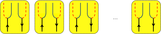
(b)

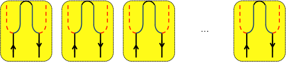
(c)

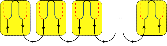
(d)

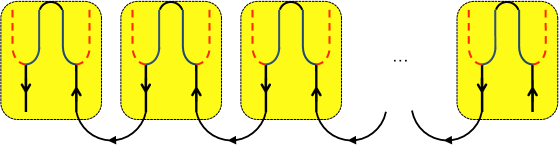
Figure 5: (Color online) (a) A chain of wires is partitioned into bundles. A bundle is depicted by a domino. The pattern in the domino corresponds to a right- and left-moving critical sector with the affine Lie algebra $\hat{g}^{\,}_{k,k^{\prime}}:=\widehat{su}(2)^{\,}_{k}\oplus\widehat{su}(2)^{\,}_{k^{\prime}}$ represented by a thick vertical like supporting an up arrow for right movers and down arrow for left movers. Its diagonal subalgebra $\hat{h}^{\,}_{k,k^{\prime}}:=\widehat{su}(2)^{\,}_{k+k^{\prime}}$ is represented by the forking into a blue solid line. The coset $\hat{g}^{\,}_{k,k^{\prime}}/\hat{h}^{\,}_{k,k^{\prime}}$ is represented by the forking into a red dashed line. (b) An arc inside each domino depicts a current-current interaction between the generators of $\hat{h}^{\,}_{k,k^{\prime}}$. These arcs gap all the critical modes generated by $\hat{h}^{\,}_{k,k^{\prime}}:=\widehat{su}(2)^{\,}_{k+k^{\prime}}$ within a bundle. (c) An arc between two consecutive dominoes depicts the current-current interactions between the generators of $\hat{g}^{\,}_{k,k^{\prime}}$. The arrows on these arcs indicate that these interactions break time-reversal symmetry. These arcs gap all remaining critical modes except for the modes generated by the right-moving $\hat{g}^{\,}_{k,k^{\prime}}/\hat{h}^{\,}_{k,k^{\prime}}$ on bundle $\texttt{m}=1$ and the modes generated by the left-moving $\hat{g}^{\,}_{k,k^{\prime}}/\hat{h}^{\,}_{k,k^{\prime}}$ on bundle $\texttt{m}=n$. (d) Reversal of time is represented by reversing all arrows.

III.3 Partial gapping without time-reversal symmetry

We have identified the continuous symmetry groups (63) and (70) for the free theory (62). In the latter case, the currents entering the Sugawara construction (72) corresponding to the symmetry group $U(2)\times\cdots\times U(2)$ obey the semi-simple affine Lie algebra

$$\hat{u}:=\operatornamewithlimits{\bigoplus}_{I=1}^{N}\hat{u}(2)^{\,}_{1}.$$ (78)

In the former case, we could also have introduced the Sugawara construction with the affine Lie algebra $\hat{u}(2N)^{\,}_{1}$ of level one which is associated to the symmetry group $U(2N)$. In fact, this was done in Appendix B.3 for the group $U(2N)\sim O(4N)$ when discussing the symmetry class AII.

We shall now consider a symmetry group (and the corresponding Sugawara construction) that is intermediate between $U(2)\times\cdots\times U(2)$ and $U(2N)$.

The idea is the following. We break the chain of $N\gg 1$ wires into $n>1$ unit cells (bundles), each of which is made of $k+k^{\prime}$ consecutive wires as is illustrated in Fig. 4. In other words, we assume that

$$N=n\,(k+k^{\prime})$$ (79)

with $k$ and $k^{\prime}$ two nonvanishing positive integers. The thermodynamic limit $N\to\infty$ is taken holding $k$ and $k^{\prime}$ fixed. The spatial range of the current-current interactions that we will use to gap partially the spectrum of the free theory (62) involves at most two consecutive bundles of $k+k^{\prime}$ wires. Locality is thus guaranteed. We assign the teletype font $\texttt{m}=1,\cdots,n$ when labeling the bundles of $k+k^{\prime}$ consecutive wires that make up an enlarged unit cell of the chain of $N$ wires. An important case corresponds to the choice $k=k^{\prime}=1$ that amounts to rearranging the chain of wires into a chain of ladders, as is depicted in Fig. 1.

The symmetry that we select when considering any one of the $n$ bundles of $k+k^{\prime}$ consecutive wires is the direct product

$$U:=U(2k)\times U(2k^{\prime}).$$ (80a)

The corresponding semi-simple affine Lie algebra is

$$\hat{u}^{\,}_{1}:=\hat{u}(2k)^{\,}_{1}\oplus\hat{u}(2k^{\prime})^{\,}_{1}.$$ (80b)

By construction, the central charges $c[\hat{u}^{\,}_{1}]$, $c[\hat{u}(2k)^{\,}_{1}]$, and $c[\hat{u}(2k^{\prime})^{\,}_{1}]$ are related by

$$c[\hat{u}^{\,}_{1}]=c[\hat{u}(2k)^{\,}_{1}]+c[\hat{u}(2k^{\prime})^{\,}_{1}].$$ (81)

As it should be

$$2N= \,2\,n\,(k+k^{\prime})$$

$$= \,n\left(c[\hat{u}(2k)^{\,}_{1}]+c[\hat{u}(2k^{\prime})^{\,}_{1}]\right)$$

$$= \,n\,c[\hat{u}^{\,}_{1}].$$ (82)

We are in position to take advantage of the non-Abelian bosonization of a bundle of $k+k^{\prime}$ consecutive wires in any of the enlarged unit cell labeled by $\texttt{m}=1,\cdots,n$ with the symmetry group $U(2k)\times U(2k^{\prime})$ making up the chain of $N$ decoupled and identical wires. To avoid heavy notation, we drop the label m when the bundles are decoupled.

Inspired by the works of Affleck and Ludwig in connection to the multichannel Kondo effect,   Affleck (1990); Affleck and Ludwig (1991a, b) we use the following generalization of the Sugawara decomposition (72), which we only present in the sector with the symmetry group $U(2k)$ without loss of generality. The identity

$$\hat{u}(2k)^{\,}_{1}=\hat{u}(1)\oplus\widehat{su}(2)^{\,}_{k}\oplus\widehat{su}(k)^{\,}_{2}$$ (83a)

between affine Lie algebras is equivalent to stating that

$$T^{\,}_{\mathrm{R}}[\hat{u}(2k)^{\,}_{1}]=T^{\,}_{\mathrm{R}}[\hat{u}(1)]+T^{\,}_{\mathrm{R}}[\widehat{su}(2)^{\,}_{k}]+T^{\,}_{\mathrm{R}}[\widehat{su}(k)^{\,}_{2}],$$ (83b)

$$T^{\,}_{\mathrm{L}}[\hat{u}(2k)^{\,}_{1}]=T^{\,}_{\mathrm{L}}[\hat{u}(1)]+T^{\,}_{\mathrm{L}}[\widehat{su}(2)^{\,}_{k}]+T^{\,}_{\mathrm{L}}[\widehat{su}(k)^{\,}_{2}],$$ (83c)

where [for simplicity we only present this relation in the right-moving sector; we also choose the multiplicative normalization from Ref. Affleck, 1990; Affleck and Ludwig, 1991a, b rather than the one in Eq. (22)]

$$T^{\,}_{\mathrm{R}}[\hat{u}(2k)^{\,}_{1}]=\frac{\mathrm{i}}{2\pi}\sum_{\alpha=1}^{2}\sum_{A=1}^{k}\psi^{*}_{\mathrm{R},\alpha,A}\,\left(\partial^{\,}_{t}-\partial^{\,}_{x}\right)\,\psi^{\,}_{\mathrm{R},\alpha,A}$$ (83d)

on the one hand, and

$$T^{\,}_{\mathrm{R}}[\hat{u}(1)]=\frac{1}{4k}\,j^{\,}_{\mathrm{R}}\,j^{\,}_{\mathrm{R}},$$ (83e)

$$T^{\,}_{\mathrm{R}}[\widehat{su}(2)^{\,}_{k}]=\frac{1}{k+2}\,\sum_{c=1}^{3}J^{c}_{\mathrm{R}}\,J^{c}_{\mathrm{R}},$$ (83f)

$$T^{\,}_{\mathrm{R}}[\widehat{su}(k)^{\,}_{2}]=\frac{1}{2+k}\,\sum_{\mathrm{c}=1}^{k^{2}-1}\mathrm{J}^{\mathrm{c}}_{\mathrm{R}}\,\mathrm{J}^{\mathrm{c}}_{\mathrm{R}},$$ (83g)

on the other hand. The currents are here defined by

$$j^{\,}_{\mathrm{R}}:=\sum_{\alpha=1}^{2}\sum_{A=1}^{k}\psi^{*}_{\mathrm{R},\alpha,A}\,\psi^{\,}_{\mathrm{R},\alpha,A},$$ (84a)

$$J^{c}_{\mathrm{R}}:=\frac{1}{2}\sum_{\alpha,\beta=1}^{2}\sum_{A=1}^{k}\psi^{*}_{\mathrm{R},\alpha,A}\ \sigma^{c}_{\alpha\beta}\ \psi^{\,}_{\mathrm{R},\beta,A},$$ (84b)

$$\mathrm{J}^{\mathrm{c}}_{\mathrm{R}}:=\sum_{\alpha=1}^{2}\sum_{A,B=1}^{k}\psi^{*}_{\mathrm{R},\alpha,A}\ T^{\mathrm{c}}_{AB}\ \psi^{\,}_{\mathrm{R},\alpha,B},$$ (84c)

for $$c=1,2,3 \mathrm{c}=1,\cdots,k^{2}-1$$ and , respectively. Hereto, we have imposed the normalization condition

$$\mathrm{tr}\,\left(T^{\mathrm{c}}\,T^{\mathrm{c}^{\prime}}\right)=\frac{1}{2}\,\delta^{\,}_{\mathrm{c}\mathrm{c}^{\prime}}$$ (84d)

for $$\mathrm{c},\mathrm{c}^{\prime}=1,\cdots,k^{2}-1 su(k)$$. This normalization condition is equivalent to choosing the structure constants of the unitary Lie algebra such that

$$\sum_{\mathrm{c}^{\prime\prime},\mathrm{c}^{\prime\prime\prime}}^{k^{2}-1}f^{\,}_{\mathrm{c}\mathrm{c}^{\prime\prime}\mathrm{c}^{\prime\prime\prime}}\,f^{\,}_{\mathrm{c}^{\prime}\mathrm{c}^{\prime\prime}\mathrm{c}^{\prime\prime\prime}}=k\,\delta^{\,}_{\mathrm{c}\mathrm{c}^{\prime}}$$ (84e)

for any $\mathrm{c},\mathrm{c}^{\prime}=1,\cdots,k^{2}-1$.

The transformation laws of the currents (84) under the representation (65) of time reversal are

$$j^{\,}_{\mathrm{R}}\mapsto+j^{\,}_{\mathrm{L}},\qquad j^{\,}_{\mathrm{L}}\mapsto+j^{\,}_{\mathrm{R}},$$ (85a)

$$J^{c}_{\mathrm{R}}\mapsto-J^{c}_{\mathrm{L}},\qquad J^{c}_{\mathrm{L}}\mapsto-J^{c}_{\mathrm{R}},$$ (85b)

$$\mathrm{J}^{\mathrm{c}}_{\mathrm{R}}\mapsto(-1)^{p(\mathrm{c})}\,\mathrm{J}^{\mathrm{c}}_{\mathrm{L}},\qquad\mathrm{J}^{\mathrm{c}}_{\mathrm{L}}\mapsto(-1)^{p(\mathrm{c})}\,\mathrm{J}^{\mathrm{c}}_{\mathrm{R}},$$ (85c)

for $c=1,2,3$ and $\mathrm{c}=1,\cdots,k^{2}-1$. Here, $p(\mathrm{c})=0$ if the generator $T^{\mathrm{c}}$ is a real-valued matrix while $p(\mathrm{c})=1$ if the generator $T^{\mathrm{c}}$ is an imaginary-valued matrix.

For any given bundle, the currents (84a), (84b), (84c), and their counterparts with $k$ replaced by $k^{\prime}$ are separately conserved, for they all commute pairwise. To each of these six pairwise commuting currents, there corresponds a gapless sector of the free theory on which these currents act. The point-split and normal-ordered Lagrangian density  

$$\begin{split}\mathcal{L}^{U(1)}_{\mathrm{int}}:=&\,-g^{\,}_{U(1)}\,e^{\mathrm{i}\alpha(x)}\,\left(\prod_{A=1}^{k}\prod_{\alpha=1}^{2}\psi^{*}_{\mathrm{R},\alpha,A}\right)\\ &\,\times\left(\prod_{A=k}^{1}\prod_{\alpha=2}^{1}\psi^{\,}_{\mathrm{L},\alpha,A}\right)\\ &\,+[\psi^{*}_{\mathrm{R}}\to\psi^{\,}_{\mathrm{L}},\ \psi^{\,}_{\mathrm{L}}\to\psi^{*}_{\mathrm{R}},\ \alpha(x)\to-\alpha(x)]\end{split}$$ (86)

gaps the $U(1)$ charge sector for the wires $1$ to $k$ from the bundle for $g^{\,}_{U(1)}>0$ sufficiently large. The $SU(2)$ current-current interaction

$$\mathcal{L}^{SU(2)}_{\mathrm{int}}:=-\lambda^{\,}_{SU(2)}\sum_{c=1}^{3}J^{c}_{\mathrm{R}}\,J^{c}_{\mathrm{L}}$$ (87)

gaps the $SU(2)$ sector for the wires $1$ to $k$ from the bundle when $\lambda^{\,}_{SU(2)}>0$. The $SU(k)$ current-current interaction

$$\mathcal{L}^{SU(k)}_{\mathrm{int}}:=-\lambda^{\,}_{SU(k)}\sum_{\mathrm{c}=1}^{k^{2}-1}\mathrm{J}^{\mathrm{c}}_{\mathrm{R}}\,\mathrm{J}^{\mathrm{c}}_{\mathrm{L}}$$ (88)

gaps the $SU(k)$ sector for the wires $1$ to $k$ from the bundle when $\lambda^{\,}_{SU(k)}>0$. The same reasoning applies in the sector with $U(2k^{\prime})$ symmetry.

We choose to gap the $U(1)$ and $SU(k)$ sectors without breaking spontaneously the $SU(k)$ symmetry, while leaving the sector of the theory associated to the symmetry

$$G:=SU(2)\times SU(2)$$ (89)

momentarily gapless. The low-energy theory is then given by the gapless theory with an energy-momentum tensor of the Sugawara form whereby the currents realize the semi-simple affine Lie algebra

$$\hat{g}^{(n)}_{k,k^{\prime}}:=\operatornamewithlimits{\bigoplus}_{\texttt{m}=1}^{n}\Bigg{(}\widehat{su}(2)^{\,}_{k}\oplus\widehat{su}(2)^{\,}_{k^{\prime}}\Bigg{)}.$$ (90)

This gapless theory has the central charge

$$c[\hat{g}^{(n)}_{k,k^{\prime}}]= \,\sum_{\texttt{m}=1}^{n}\Bigg{(}c[\widehat{su}(2)^{\,}_{k}]+c[\widehat{su}(2)^{\,}_{k^{\prime}}]\Bigg{)}$$

$$= \,3\,n\,\Bigg{(}\frac{k}{k+2}+\frac{k^{\prime}}{k^{\prime}+2}\Bigg{)}.$$ (91)

As it should be, this central charge is smaller than the central charge $2\,n\,(k+k^{\prime})$ from Eq. (64).

We consider the diagonal subgroup

$$H:=SU(2)$$ (92)

of the group (89). The corresponding semi-simple affine Lie algebra, a semi-simple affine subalgebra of $\hat{g}^{\,}_{k,k^{\prime}}$, is

$$\hat{h}^{(n)}_{k,k^{\prime}}:=\operatornamewithlimits{\bigoplus}_{\texttt{m}=1}^{n}\widehat{su}(2)^{\,}_{k+k^{\prime}}.$$ (93)

We need to reinstate the label $\texttt{m}=1,\cdots,n$ for the bundles of $k+k^{\prime}$ consecutive wires as well as the left- and right-moving labels as we are going to couple these sectors. We denote the generators of $\hat{g}^{(n)}_{k,k^{\prime}}$ by $\mathcal{J}^{\mathcal{A}}_{\mathrm{R},\texttt{m}}$ and $\mathcal{J}^{\mathcal{A}}_{\mathrm{L},\texttt{m}}$, where $\mathcal{A}=1,\cdots,6$ and $\texttt{m}=1,\cdots,n$. For example, in the right-moving sector, we may choose the vector field

$$\bm{\mathcal{J}}^{\,}_{\mathrm{R},\texttt{m}}:=\frac{1}{2}\sum_{\alpha,\beta=1}^{2}\sum_{A=1}^{k}\psi^{*}_{\mathrm{R},\alpha,A,\texttt{m}}\ \bm{\sigma}^{\,}_{\alpha\beta}\ \psi^{\,}_{\mathrm{R},\beta,A,\texttt{m}},$$ (94a)

when $$\mathcal{A}=1,2,3$$ and the vector-field

$$\bm{\mathcal{J}}^{\prime}_{\mathrm{R},\texttt{m}}:=\frac{1}{2}\sum_{\alpha,\beta=1}^{2}\sum_{A^{\prime}=1}^{k^{\prime}}\psi^{*}_{\mathrm{R},\alpha,A^{\prime},\texttt{m}}\ \bm{\sigma}^{\,}_{\alpha\beta}\ \psi^{\,}_{\mathrm{R},\beta,A^{\prime},\texttt{m}},$$ (94b)

when $$\mathcal{A}=4,5,6 \hat{h}^{(n)}_{k,k^{\prime}} \mathcal{K}^{\mathcal{B}}_{\mathrm{R},\texttt{m}} \mathcal{K}^{\mathcal{B}}_{\mathrm{L},\texttt{m}} \mathcal{B}=1,\cdots,3 \texttt{m}=1,\cdots,n$$. We denote the generators of by and , where and . For example, in the right-moving sector, we may choose the vector field

$$\bm{\mathcal{K}}^{\,}_{\mathrm{R},\texttt{m}}:=\bm{\mathcal{J}}^{\,}_{\mathrm{R},\texttt{m}}+\bm{\mathcal{J}}^{\prime}_{\mathrm{R},\texttt{m}}.$$ (94c)

We work with open boundary conditions along the chain of quantum wires and define the interaction [see Fig. 5(c)]

$$\begin{split}\mathcal{L}^{\mathrm{L}\to\mathrm{R}}_{\mathrm{int}}:=&\,-\sum_{\texttt{m}=1}^{n-1}\sum_{\mathcal{A}=1}^{6}\lambda^{\mathcal{A}}_{\texttt{m}}\,\mathcal{J}^{\mathcal{A}}_{\mathrm{L},\texttt{m}}\,\mathcal{J}^{\mathcal{A}}_{\mathrm{R},\texttt{m}+1}\\ &\,-\sum_{\texttt{m}=1}^{n}\sum_{\mathcal{B}=1}^{3}\upsilon^{\mathcal{B}}_{\texttt{m}}\,\mathcal{K}^{\mathcal{B}}_{\mathrm{L},\texttt{m}}\,\mathcal{K}^{\mathcal{B}}_{\mathrm{R},\texttt{m}},\end{split}$$ (94d)

where the couplings $\lambda^{\mathcal{A}}_{\texttt{m}}$ and $\upsilon^{\mathcal{B}}_{\texttt{m}}$ are real-valued. Had we imposed periodic boundary conditions in the direction of the chain of wires on the Grassmann fields, it would be legitimate to extend the sum over the bundles so as to include the term with $\texttt{m}=n$.

It is shown in Appendix C.2 that (i) all couplings in Eq. (94d) flow to strong coupling when initially nonvanishing and positive, (ii) no new terms involving the right-moving generators from $\hat{g}^{(n)}_{k,k^{\prime}}/\hat{h}^{(n)}_{k,k^{\prime}}$ in the bundle $\texttt{m}=1$ appear to one loop, and (iii) no new terms involving the left-moving generators from $\hat{g}^{(n)}_{k,k^{\prime}}/\hat{h}^{(n)}_{k,k^{\prime}}$ in the bundle $\texttt{m}=n$ appear to one loop.

We make the following conjecture regarding the strong coupling fixed point depending on the initial values of the couplings in Eq. (94d).

With open boundary conditions and when all the couplings in Eq. (94d) are positive and of the same order, the resulting theory remains critical. As the resulting theory would be fully gapped had we opted for periodic boundary conditions, the critical sectors of the theory with open boundary conditions must be confined to the boundaries, namely the first bundle $\texttt{m}=1$ and the last bundle $\texttt{m}=n$. The first bundle of $k+k^{\prime}$ wires hosts the critical theory described by the right sector of the coset theory

$$\hat{g}^{\,}_{k,k^{\prime}}/\hat{h}^{\,}_{k,k^{\prime}}:=\widehat{su}^{\,}(2)^{\,}_{k}\oplus\widehat{su}^{\,}(2)^{\,}_{k^{\prime}}/\widehat{su}^{\,}(2)^{\,}_{k+k^{\prime}}$$ (95a)

with the chiral central charge

$$c[(\hat{g}^{\,}_{k,k^{\prime}}/\hat{h}^{\,}_{k,k^{\prime}})^{\,}_{\mathrm{R}}]= \,3\,\Bigg{(}\frac{k}{k+2}+\frac{k^{\prime}}{k^{\prime}+2}\Bigg{)}-3\,\frac{k+k^{\prime}}{k+k^{\prime}+2}$$

$$= \,1-\frac{6k^{\prime}}{(k+2)(k+k^{\prime}+2)}+\frac{2(k^{\prime}-1)}{k^{\prime}+2}.$$ (95b)

The last bundle of $$k+k^{\prime}$$ wires hosts the critical theory described by the left sector of the coset theory

$$\hat{g}^{\,}_{k,k^{\prime}}/\hat{h}^{\,}_{k,k^{\prime}}:=\widehat{su}^{\,}(2)^{\,}_{k}\oplus\widehat{su}^{\,}(2)^{\,}_{k^{\prime}}/\widehat{su}^{\,}(2)^{\,}_{k+k^{\prime}}$$ (95c)

with the chiral central charge

$$c[(\hat{g}^{\,}_{k,k^{\prime}}/\hat{h}^{\,}_{k,k^{\prime}})^{\,}_{\mathrm{L}}]= \,c[(\hat{g}^{\,}_{k,k^{\prime}}/\hat{h}^{\,}_{k,k^{\prime}})^{\,}_{\mathrm{R}}].$$ (95d)

The interaction (94d) has broken the time-reversal symmetry, gapped the bulk, and left in the first and last bundle two massless coset theories of opposite chiralities. For the bundle on the left (right) boundary the critical boundary theory is built from the holomorphic (antiholomorphic) generators in the quotient $\widehat{su}(2)^{\,}_{k}\oplus\widehat{su}(2)^{\,}_{k^{\prime}}/\widehat{su}(2)^{\,}_{k+k^{\prime}}$ of affine Lie algebras.

The last term on the right-hand side of Eqs. (95b) and (95d) is the central charge

$$c[\widehat{su}(2)^{\,}_{k^{\prime}}/\hat{u}(1)]=\frac{3\,k^{\prime}}{k^{\prime}+2}-1=\frac{2(k^{\prime}-1)}{k^{\prime}+2}$$ (96)

of the coset $\widehat{su}(2)^{\,}_{k^{\prime}}/\hat{u}(1)$. In the local operator content of this theory, one finds a pair of local parafermionic fields $\hat{\psi}^{{\dagger}}_{\mathrm{par}}$ and $\hat{\psi}^{\,}_{\mathrm{par}}$ with the scaling dimensions $(k^{\prime}-1)/k^{\prime}$ and a real-valued bosonic field $\hat{\varphi}$ such that the generators of the affine Lie algebra $\widehat{su}(2)^{\,}_{k^{\prime}}$ are represented by the operators  

$$\hat{J}^{+}(z)=\sqrt{k^{\prime}}\ \hat{\psi}^{\,}_{\mathrm{par}}(z)\,:e^{+\mathrm{i}\sqrt{2/k^{\prime}}\,\hat{\varphi}(z)}:,$$ (97a)

$$\hat{J}^{-}(z)=\sqrt{k^{\prime}}\ \hat{\psi}^{{\dagger}}_{\mathrm{par}}(z)\,:e^{-\mathrm{i}\sqrt{2/k^{\prime}}\,\hat{\varphi}(z)}:,$$ (97b)

$$\hat{J}^{0}(z)=\mathrm{i}\sqrt{2k^{\prime}}\,(\partial^{\,}_{z}\hat{\varphi})(z).$$ (97c)

For $k^{\prime}=1$, the parafermions reduce to the identity. For $k^{\prime}=2$, the parafermions obey the fermion algebra. For $k^{\prime}>2$ the parafermions obey a more complicated algebra. For example, if one writes

$$\hat{\psi}^{\,}_{\mathrm{par}}\propto\frac{\mathrm{i}}{2}\left[\hat{\chi}^{\,}_{1}+\left(\hat{\chi}^{\,}_{1}\right)^{k^{\prime}-1}\right]+\frac{1}{2}\left[\hat{\chi}^{\,}_{2}+\left(\hat{\chi}^{\,}_{2}\right)^{k^{\prime}-1}\right],$$ (98a)

it then follows that

$$\left(\hat{\chi}^{\,}_{1}\right)^{k^{\prime}}=1,\qquad\left(\hat{\chi}^{\,}_{2}\right)^{k^{\prime}}=1,$$ (98b)

$$\left(\hat{\chi}^{\,}_{1}\right)^{k^{\prime}-1}=\left(\hat{\chi}^{\,}_{1}\right)^{{\dagger}},\qquad\left(\hat{\chi}^{\,}_{2}\right)^{k^{\prime}-1}=\left(\hat{\chi}^{\,}_{2}\right)^{{\dagger}},$$ (98c)

$$\hat{\chi}^{\,}_{1}\,\hat{\chi}^{\,}_{2}=e^{\mathrm{i}2\pi/k^{\prime}}\,\hat{\chi}^{\,}_{2}\,\hat{\chi}^{\,}_{1},$$ (98d)

holds locally.

It is time to specialize by choosing

$$k^{\prime}=1.$$ (99)

With this choice, the chiral central charges (95b) and (95d) are nothing but the central charge

$$c(k)=1-\frac{6}{(k+2)(k+3)}$$ (100)

for the minimal models of two-dimensional conformal field theories. This is not a coincidence, for it is known that the coset affine Lie algebra

$$\hat{g}^{\,}_{k,1}/\hat{h}^{\,}_{k,1}=\widehat{su}(2)^{\,}_{k}\oplus\widehat{su}(2)^{\,}_{1}/\widehat{su}(2)^{\,}_{k+1}$$ (101)

realizes the series of minimal models with $k=1,2,\cdots$.   Di Francesco et al. (1997) The minimal models encode the critical properties of two-dimensional lattice models at their critical temperature such as the Ising model ($k=1$), the tricritical Ising model ($k=2$), the three-states Potts model ($k=3$), and so on. We conclude that we have realized the holomorphic and antiholomorphic critical sectors of the minimal models on the opposite boundaries of an open chain of $n$ bundles of wires, respectively.

Figure 6: One possible phase diagram with the interaction (105). The time-reversal symmetric point is parametrized by $\kappa=0$. The vertical axis is the many-body gap between the ground state and all excited states when periodic boundary conditions are imposed. The continuous line represents the scenario for an exotic spin-liquid quantum critical point. The dashed line represents the scenario for a first-order quantum phase transition. The signs $-$ and $+$ distinguish the two ground states that evolve adiabatically as $\kappa\neq 0$ changes and cross precisely at $\kappa=0$.

The choice $k^{\prime}=2$ turns the chiral central charges (95b) and (95d) into the chiral central charge

$$c(k)=\frac{3}{2}\Biggl{[}1-\frac{8}{(k+2)(k+4)}\Biggr{]}$$ (102)

for the minimal models of two-dimensional superconformal field theories. This is again not a coincidence, for it is known that the coset affine Lie algebra

$$\hat{g}^{\,}_{k,2}/\hat{h}^{\,}_{k,2}=\widehat{su}(2)^{\,}_{k}\oplus\widehat{su}(2)^{\,}_{2}/\widehat{su}(2)^{\,}_{k+2}$$ (103)

realizes the series of superconformal minimal models with $k=1,2,\cdots$.   Di Francesco et al. (1997) Notice that, for $k=1$, $c(k=1)=7/10$ coincides with the second member ($k=2$) of the minimal model (100) that corresponds to the tricritical Ising model. The tricritical Ising model is one example that realizes supersymmetry in statistical physics. We conclude that we have realized the holomorphic and antiholomorphic critical sectors of the superconformal minimal models on the opposite boundaries of an open chain of $n$ bundles of wires, respectively.

III.4 Partial gapping with time-reversal symmetry

We shall impose time-reversal symmetry on the array of quantum wires coupled by current-current interactions in three different ways.

In Sec. III.4.1, we symmetrize the interaction (94d) under reversal of time.

In Sec. III.4.2, we double the number of degrees of freedom in the low-energy sector of the theory by postulating that this doubling originates from degrees of freedom that are exchanged under reversal of time. We then write down current-current interactions that preserve time-reversal symmetry, gap the bulk, but leave gapless boundary states.

In Sec. III.4.3, unlike was the case in Secs. III.3, III.4.1, and III.4.2, we assume that spin-1/2 rotation symmetry is broken prior to adding current-current interactions. We then explain how to reproduce the treatment of Sec. III.4.2.

III.4.1 Case I – Symmetrized interaction

We assume that the interactions responsible for gapping the $U(k)\times U(k^{\prime})$ sector of the theory in Sec. III.3 preserve both time-reversal symmetry and spin-1/2 rotation symmetry.

(a)                                                                                 

(b)                                                                                 

Figure 7: For the case when the phases transitions in the range $-1\leq\kappa\leq+1$ at strong values of the couplings $\lambda^{\mathcal{A}}_{\texttt{m}}>0$ and $v^{\mathcal{B}}_{\texttt{m}}>0$ in Eq. (105) are continuous, the critical point at $\kappa=0$ is either unstable or stable depending on whether the number of critical points for $-1<\kappa<0$ is even as in (a) or odd as in (b), respectively.

Reversal of time turns the interaction (94d) into the interaction [see Fig. 5(d)]

$$\begin{split}\mathcal{L}^{\mathrm{R}\to\mathrm{L}}_{\mathrm{int}}:=&\,-\sum_{\texttt{m}=1}^{n-1}\sum_{\mathcal{A}=1}^{6}\lambda^{\mathcal{A}}_{\texttt{m}}\,\mathcal{J}^{\mathcal{A}}_{\mathrm{R},\texttt{m}}\,\mathcal{J}^{\mathcal{A}}_{\mathrm{L},\texttt{m}+1}\\ &\,-\sum_{\texttt{m}=1}^{n}\sum_{\mathcal{B}=1}^{3}\upsilon^{\mathcal{B}}_{\texttt{m}}\,\mathcal{K}^{\mathcal{B}}_{\mathrm{R},\texttt{m}}\,\mathcal{K}^{\mathcal{B}}_{\mathrm{L},\texttt{m}}.\end{split}$$ (104)

As was the case with the interaction (94d), we conjecture a gapped bulk with two massless coset theories of opposite chiralities on the first and last bundles of wires. For the left (right) boundary bundle the critical boundary theory is built from the antiholomorphic (holomorphic) generators in the quotient $\widehat{su}(2)^{\,}_{k}\oplus\widehat{su}(2)^{\,}_{k^{\prime}}/\widehat{su}(2)^{\,}_{k+k^{\prime}}$ of affine Lie algebras.

We may then interpolate between the interactions (94d) and (104) as a function of the real-valued parameter $\kappa$ by defining

$$\mathcal{L}^{\,}_{\mathrm{int}}(\kappa):=\frac{1-\kappa}{2}\,\mathcal{L}^{\mathrm{L}\to\mathrm{R}}_{\mathrm{int}}+\frac{1+\kappa}{2}\,\mathcal{L}^{\mathrm{R}\to\mathrm{L}}_{\mathrm{int}}.$$ (105)

The interactions (94d) and (104) compete to impose one of two ways for the breaking of time-reversal symmetry. When $\kappa\leq-1$, the interaction $\mathcal{L}^{\mathrm{L}\to\mathrm{R}}_{\mathrm{int}}$ is marginally relevant, while the interaction $\mathcal{L}^{\mathrm{R}\to\mathrm{L}}_{\mathrm{int}}$ is marginally irrelevant, as is shown in Appendix C.3. It is the fixed point represented by Fig. 5(c) to which the relevant couplings flow. When $1\leq\kappa$, it is the fixed point represented by Fig. 5(d) to which the relevant couplings flow as is shown in Appendix C.3. The analysis of the one-loop RG flows is more subtle when $\kappa\in[-1,+1]\setminus\{0\}$. It is shown in Appendix C.3 that $\mathcal{L}^{\mathrm{L}\to\mathrm{R}}_{\mathrm{int}}$ and $\mathcal{L}^{\mathrm{R}\to\mathrm{L}}_{\mathrm{int}}$ are both marginally relevant perturbations. If one assumes that the point $\kappa=0$ at which time-reversal symmetry holds explicitly is singular, there are then two logical possibilities pertaining to the nature of this singularity.

On the one hand, the singularity at $\kappa=0$ could signal a continuous quantum phase transition at which the bulk gap closes and the (thermal) Hall conductivity switches sign, as occurs with the single-particle Dirac Hamiltonian   Ludwig et al. (1994)

$$\mathcal{H}^{\,}_{\mathrm{D}}:=-\mathrm{i}\sigma^{\,}_{x}\,\hat{p}^{\,}_{x}-\mathrm{i}\sigma^{\,}_{y}\,\hat{p}^{\,}_{y}+m\,\sigma^{\,}_{z}$$ (106)

in two-dimensional space when the mass $m$ changes sign in a continuous fashion. If so, the gapless bulk phase represents an exotic gapless spin liquid phase in $(2+1)$-dimensional space and time, for it emerges from two long-ranged entangled gapped phases supporting non-Abelian topological order that are unrelated by a breaking of a local symmetry.

If all phase transitions in the range $-1\leq\kappa\leq+1$ are continuous, the critical point at $\kappa=0$ is either stable or unstable. The latter case occurs if the number of critical points in the range $-1<\kappa<0$ is even, as shown in Figs. 7(a). The former case occurs if the number of critical points in the range $-1<\kappa<0$ is odd, as shown in Figs. 7(b). The one-loop RG analysis made in Appendix C.3 applies to the vicinity of the noninteracting critical point when all the couplings $\lambda^{\mathcal{A}}_{\texttt{m}}$ and $v^{\mathcal{B}}_{\texttt{m}}$ in Eq. (105) vanish. In the limit $\lambda^{\mathcal{A}}_{\texttt{m}}\to 0$ and $v^{\mathcal{B}}_{\texttt{m}}\to 0$, the one-loop RG flow for $\kappa$ is the one depicted in Fig. 7(a). However, we cannot infer from this weak coupling analysis whether it is Fig. 7(a) or Fig. 7(b) that applies to the relevant limit $\lambda^{\mathcal{A}}_{\texttt{m}}\to\infty$ and $v^{\mathcal{B}}_{\texttt{m}}\to\infty$.

On the other hand, the singularity at $\kappa=0$ could signal a discontinuous transition, as occurs in the Ising model upon changing the sign of an applied magnetic field. At $\kappa=0$, the energy eigenvalue of the ground state for $\kappa<0$ crosses that of the ground state for $\kappa>0$, while the gap to the excitation spectra for $\kappa<0$ and $\kappa>0$ do not close at $\kappa=0$.

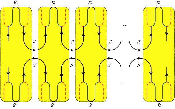
Figure 8: (Color online) Chain of $N$ wires, each wire supporting four right- and four left-moving flavors, that are coupled by current-current interactions in a way that is explicitly symmetric under reversal of time. A bundle of $8\times(k+k^{\prime})$ right- or left-moving electronic degrees of freedom is represented by a domino. There are $n=N/(k+k^{\prime})$ dominoes. The currents denoted by $\mathcal{J}$ generate the affine Lie algebra $\widehat{su}(2)^{\,}_{k}\oplus\widehat{su}(2)^{\,}_{k^{\prime}}$. The currents denoted by $\mathcal{K}$ generate the affine Lie algebra $\widehat{su}(2)^{\,}_{k+k^{\prime}}$. The currents denoted by $\tilde{\mathcal{J}}$ generate the affine Lie algebra $\widehat{\widetilde{su}}(2)^{\,}_{k}\oplus\widehat{\widetilde{su}}(2)^{\,}_{k^{\prime}}$. The currents denoted by $\tilde{\mathcal{K}}$ generate the affine Lie algebra $\widehat{\widetilde{su}}(2)^{\,}_{k+k^{\prime}}$.

III.4.2 Case II – Doubled degrees of freedom

We continue assuming that the interactions responsible for gapping the $U(k)\times U(k^{\prime})$ sector of the theory in Sec. III.3 preserve both time-reversal symmetry and spin-1/2 rotation symmetry.

An alternative implementation of time-reversal symmetry consists in (i) doubling the dimensionality of the Fock space by direct product with a two-dimensional auxiliary Hilbert space and (ii) demanding that reversal of time is represented by a matrix that is off-diagonal with respect to this auxiliary two-dimensional Hilbert space. An example of such a two-dimensional auxiliary Hilbert space is provided by the two valleys of graphene [recall Example 2 of a quasi-one-dimensional gapless phase defined by Eq. (67)]. According to Eq. (67), half of the degrees of freedom encoded in any one of the bundles can be interpreted as originating from the two-dimensional nonvanishing momenta about which the low-energy degrees of freedom are constructed.

Accordingly, we may choose to work with the total of $8\times N$ electronic right- or left-moving degrees of freedom, which we organize into $n$ bundles, each of which supports $8\times(k+k^{\prime})$ electronic right- or left-moving degrees of freedom, where $k$ and $k^{\prime}$ are two nonvanishing positive integers. In other words, the number $4\times N=4\times n\,(k+k^{\prime})$ of electronic right- or left-moving degrees of freedom corresponding to the number of quantum wires (79) is replaced by

$$8\times N=8n\,(k+k^{\prime}).$$ (107)

This is to say that we extend the quadruplet of Grassmann-valued vectors $\psi^{*}_{\mathrm{R}}$, $\psi^{*}_{\mathrm{L}}$, $\psi^{\,}_{\mathrm{R}}$, and $\psi^{\,}_{\mathrm{L}}$ with the components $\psi^{*}_{\mathrm{R},\sigma,I}$, $\psi^{*}_{\mathrm{L},\sigma,I}$, $\psi^{\,}_{\mathrm{R},\sigma,I}$, and $\psi^{\,}_{\mathrm{L},\sigma,I}$, respectively, by the quadruplet of Grassmann-valued vectors $\tilde{\psi}^{*}_{\mathrm{R}}$, $\tilde{\psi}^{*}_{\mathrm{L}}$, $\tilde{\psi}^{\,}_{\mathrm{R}}$, and $\tilde{\psi}^{\,}_{\mathrm{L}}$ with the components $\tilde{\psi}^{*}_{\mathrm{R},\sigma,I}$, $\tilde{\psi}^{*}_{\mathrm{L},\sigma,I}$, $\tilde{\psi}^{\,}_{\mathrm{R},\sigma,I}$, and $\tilde{\psi}^{\,}_{\mathrm{L},\sigma,I}$, respectively. We then replace the critical theory (62) by the critical theory

$$\begin{split}\mathcal{L}^{\,}_{0}:=&\,\mathrm{i}\Big{[}\psi^{*\mathsf{T}}_{\mathrm{R}}\,(\partial^{\,}_{t}+\partial^{\,}_{x})\,\psi^{\,}_{\mathrm{R}}+\psi^{*\mathsf{T}}_{\mathrm{L}}\,(\partial^{\,}_{t}-\partial^{\,}_{x})\,\psi^{\,}_{\mathrm{L}}\Big{]}\\ &\,+\mathrm{i}\Big{[}\tilde{\psi}^{*\mathsf{T}}_{\mathrm{R}}\,(\partial^{\,}_{t}+\partial^{\,}_{x})\,\tilde{\psi}^{\,}_{\mathrm{R}}+\tilde{\psi}^{*\mathsf{T}}_{\mathrm{L}}\,(\partial^{\,}_{t}-\partial^{\,}_{x})\,\tilde{\psi}^{\,}_{\mathrm{L}}\Big{]}\end{split}$$ (108a)

with the action

$$S^{\,}_{0}:=\int\mathrm{d}t\int\mathrm{d}x\,\mathcal{L}^{\,}_{0}$$ (108b)

and the partition function

$$Z^{\,}_{0}:=\int\mathcal{D}[\psi^{*},\psi]\ \int\mathcal{D}[\tilde{\psi}^{*},\tilde{\psi}]\ e^{\mathrm{i}S^{\,}_{0}}.$$ (108c)

Reversal of time is the antilinear transformation defined by the fundamental rules

$$\psi^{*}_{\mathrm{R},\uparrow,I}\mapsto+\tilde{\psi}^{*}_{\mathrm{L},\downarrow,I},\qquad\psi^{*}_{\mathrm{R},\downarrow,I}\mapsto-\tilde{\psi}^{*}_{\mathrm{L},\uparrow,I},$$ (109a)

$$\psi^{*}_{\mathrm{L},\uparrow,I}\mapsto+\tilde{\psi}^{*}_{\mathrm{R},\downarrow,I},\qquad\psi^{*}_{\mathrm{L},\downarrow,I}\mapsto-\tilde{\psi}^{*}_{\mathrm{R},\uparrow,I},$$ (109b)

$$\tilde{\psi}^{*}_{\mathrm{R},\uparrow,I}\mapsto+\psi^{*}_{\mathrm{L},\downarrow,I},\qquad\tilde{\psi}^{*}_{\mathrm{R},\downarrow,I}\mapsto-\psi^{*}_{\mathrm{L},\uparrow,I},$$ (109c)

$$\tilde{\psi}^{*}_{\mathrm{L},\uparrow,I}\mapsto+\psi^{*}_{\mathrm{R},\downarrow,I},\qquad\tilde{\psi}^{*}_{\mathrm{L},\downarrow,I}\mapsto-\psi^{*}_{\mathrm{R},\uparrow,I},$$ (109d)

and

$$\psi^{\,}_{\mathrm{R},\uparrow,I}\mapsto+\tilde{\psi}^{\,}_{\mathrm{L},\downarrow,I},\qquad\psi^{\,}_{\mathrm{R},\downarrow,I}\mapsto-\tilde{\psi}^{\,}_{\mathrm{L},\uparrow,I},$$ (109e)

$$\psi^{\,}_{\mathrm{L},\uparrow,I}\mapsto+\tilde{\psi}^{\,}_{\mathrm{R},\downarrow,I},\qquad\psi^{\,}_{\mathrm{L},\downarrow,I}\mapsto-\tilde{\psi}^{\,}_{\mathrm{R},\uparrow,I},$$ (109f)

$$\tilde{\psi}^{\,}_{\mathrm{R},\uparrow,I}\mapsto+\psi^{\,}_{\mathrm{L},\downarrow,I},\qquad\tilde{\psi}^{\,}_{\mathrm{R},\downarrow,I}\mapsto-\psi^{\,}_{\mathrm{L},\uparrow,I},$$ (109g)

$$\tilde{\psi}^{\,}_{\mathrm{L},\uparrow,I}\mapsto+\psi^{\,}_{\mathrm{R},\downarrow,I},\qquad\tilde{\psi}^{\,}_{\mathrm{L},\downarrow,I}\mapsto-\psi^{\,}_{\mathrm{R},\uparrow,I}.$$ (109h)

By this definition, reversal of time squares to minus the identity and leaves the critical theory (108) invariant. Moreover, if we define the Grassmann-valued doublets

$$\Psi^{*}_{\mathrm{R}}:=\begin{pmatrix}\psi^{*}_{\mathrm{R}}\\ \\ \tilde{\psi}^{*}_{\mathrm{R}}\end{pmatrix},\qquad\Psi^{*}_{\mathrm{L}}:=\begin{pmatrix}\psi^{*}_{\mathrm{L}}\\ \\ \tilde{\psi}^{*}_{\mathrm{L}}\end{pmatrix}$$ (110a)

and

$$\Psi^{\,}_{\mathrm{R}}:=\begin{pmatrix}\psi^{\,}_{\mathrm{R}}\\ \\ \tilde{\psi}^{\,}_{\mathrm{R}}\end{pmatrix},\qquad\Psi^{\,}_{\mathrm{L}}:=\begin{pmatrix}\psi^{\,}_{\mathrm{L}}\\ \\ \tilde{\psi}^{\,}_{\mathrm{L}}\end{pmatrix},$$ (110b)

the representation

$$\mathcal{L}^{\,}_{0}=\mathrm{i}\Psi^{*\mathsf{T}}_{\mathrm{R}}\left(\partial^{\,}_{t}+\partial^{\,}_{x}\right)\Psi^{\,}_{\mathrm{R}}+\mathrm{i}\Psi^{*\mathsf{T}}_{\mathrm{L}}\left(\partial^{\,}_{t}-\partial^{\,}_{x}\right)\Psi^{\,}_{\mathrm{L}}$$ (110c)

of the critical theory (108) makes it explicit that it has the symmetry group $U^{\,}_{\mathrm{R}}(4N)\times U^{\,}_{\mathrm{L}}(4N)$.

Any one bundle of $8\times(k+k^{\prime})$ electronic right- or left-moving degrees of freedom is represented by any one domino from Fig. 8. The symmetry that we select when considering any one of the $n$ bundles of $8\times(k+k^{\prime})$ electronic right- or left-moving degrees of freedom is the direct product

$$U:=\Big{(}U(2k)\times\widetilde{U}(2k)\Big{)}\times\Big{(}U(2k^{\prime})\times\widetilde{U}(2k^{\prime})\Big{)}.$$ (111a)

As before, the multiplicative factor of $$2 2k 2k^{\prime} 2 8\times n\,(k+k^{\prime}) 2k 2k^{\prime}$$ in or stands for the electronic spin-1/2 degrees of freedom. However, a second multiplicative factor of in is responsible for the two copies of the unitary group of -dimensional matrices and -dimensional matrices, respectively. The corresponding semi-simple affine Lie algebra is

$$\hat{u}^{\,}_{1}:=\Big{(}\hat{u}(2k)^{\,}_{1}\oplus\hat{\tilde{u}}(2k)^{\,}_{1}\Big{)}\oplus\Big{(}\hat{u}(2k^{\prime})^{\,}_{1}\oplus\hat{\tilde{u}}(2k^{\prime})^{\,}_{1}\Big{)}.$$ (111b)

Equation (111) should be compared to Eq. (80). As before, we use the conformal embedding

$$\hat{u}(2k)^{\,}_{1}=\hat{u}(1)\oplus\widehat{su}(2)^{\,}_{k}\oplus\widehat{su}(k)^{\,}_{2},$$ (112a)

$$\hat{\tilde{u}}(2k)^{\,}_{1}=\hat{\tilde{u}}(1)\oplus\widehat{\widetilde{su}}(2)^{\,}_{k}\oplus\widehat{\widetilde{su}}(k)^{\,}_{2},$$ (112b)

$$\hat{u}(2k^{\prime})^{\,}_{1}=\hat{u}(1)\oplus\widehat{su}(2)^{\,}_{k^{\prime}}\oplus\widehat{su}(k^{\prime})^{\,}_{2},$$ (112c)

$$\hat{\tilde{u}}(2k^{\prime})^{\,}_{1}=\hat{\tilde{u}}(1)\oplus\widehat{\widetilde{su}}(2)^{\,}_{k^{\prime}}\oplus\widehat{\widetilde{su}}(k^{\prime})^{\,}_{2},$$ (112d)

between affine Lie algebras. Here, the generators of these affine Lie algebra are given by Eq. (84) for the conformal embedding (112a), by

$$\tilde{j}^{\,}_{\mathrm{R}}:=\sum_{\alpha=1}^{2}\sum_{A=1}^{k}\tilde{\psi}^{*}_{\mathrm{R},\alpha,A}\,\tilde{\psi}^{\,}_{\mathrm{R},\alpha,A},$$ (113a)

$$\tilde{J}^{c}_{\mathrm{R}}:=\frac{1}{2}\sum_{\alpha,\beta=1}^{2}\sum_{A=1}^{k}\tilde{\psi}^{*}_{\mathrm{R},\alpha,A}\ \sigma^{c}_{\alpha\beta}\ \tilde{\psi}^{\,}_{\mathrm{R},\beta,A},$$ (113b)

$$\tilde{\mathrm{J}}^{\mathrm{c}}_{\mathrm{R}}:=\sum_{\alpha=1}^{2}\sum_{A,B=1}^{k}\tilde{\psi}^{*}_{\mathrm{R},\alpha,A}\ T^{\mathrm{c}}_{AB}\ \tilde{\psi}^{\,}_{\mathrm{R},\alpha,B},$$ (113c)

($c=1,2,3$ and $\mathrm{c}=1,\cdots,k^{2}-1$) for the conformal embedding (112b), and similarly for the conformal embeddings (112c) and (112d), respectively.

We choose to gap the sectors with the symmetries $U(1)$, $SU(k)$, $\widetilde{U}(1)$, $\widetilde{SU}(k)$, and similarly for $k^{\prime}$, while leaving the sector of the theory associated to the symmetry

$$G:=\Big{(}SU(2)\times\widetilde{SU}(2)\Big{)}\times\Big{(}SU(2)\times\widetilde{SU}(2)\Big{)}$$ (114a)

momentarily gapless. The semi-simple affine Lie algebra associated to $$G$$ is

$$\hat{g}^{(n)}_{k,k^{\prime}}=\operatornamewithlimits{\bigoplus}_{\texttt{m}=1}^{n}\Big{(}\widehat{su}(2)^{\,}_{k}\oplus\widehat{\widetilde{su}}(2)^{\,}_{k}\Big{)}\oplus\Big{(}\widehat{su}(2)^{\,}_{k^{\prime}}\oplus\widehat{\widetilde{su}}(2)^{\,}_{k^{\prime}}\Big{)}.$$ (114b)

It is now the diagonal subgroup

$$H:=SU(2)\times\widetilde{SU}(2)$$ (115a)

of the group (114a) that we shall use to construct the gapless theory on the edge. The corresponding simple affine subalgebra of $$\hat{g}^{\,}_{k,k^{\prime}}$$, is

$$\hat{h}^{(n)}_{k,k^{\prime}}:=\operatornamewithlimits{\bigoplus}_{\texttt{m}=1}^{n}\widehat{su}(2)^{\,}_{k+k^{\prime}}\oplus\widehat{\widetilde{su}}(2)^{\,}_{k+k^{\prime}}.$$ (115b)

The currents generating $\widehat{su}(2)^{\,}_{k}\oplus\widehat{su}(2)^{\,}_{k^{\prime}}$ are represented by the symbol $J$ in Fig. 8. The currents generating $\widehat{\widetilde{su}}(2)^{\,}_{k}\oplus\widehat{\widetilde{su}}(2)^{\,}_{k^{\prime}}$ are represented by the symbol $\tilde{J}$ in Fig. 8. The currents generating $\widehat{su}(2)^{\,}_{k+k^{\prime}}$ are represented by the symbol $K$ in Fig. 8. The currents generating $\widehat{\widetilde{su}}(2)^{\,}_{k+k^{\prime}}$ are represented by the symbol $\tilde{K}$ in Fig. 8.

Current-current interactions are represented in Fig. 8 by arcs that are directed when they involve the currents $J$ or $\tilde{J}$, while they are undirected when they involve the currents $K$ or $\tilde{K}$. In Fig. 8, the action of reversal of time is twofold. First, the directions of arrows must be reversed, thereby interchanging right- or left-movers. Second, the letters without $\tilde{\hphantom{J}}$ acquire a $\tilde{\hphantom{J}}$, while letters with $\tilde{\hphantom{J}}$ loose their $\tilde{\hphantom{J}}$. The corresponding interaction

$$\begin{split}\mathcal{L}^{\,}_{\mathrm{int}}:=&\,-\sum_{\texttt{m}=1}^{n-1}\sum_{\mathcal{A}=1}^{6}\lambda^{\mathcal{A}}_{\texttt{m}}\,\mathcal{J}^{\mathcal{A}}_{\mathrm{L},\texttt{m}}\,\mathcal{J}^{\mathcal{A}}_{\mathrm{R},\texttt{m}+1}-\sum_{\texttt{m}=1}^{n}\sum_{\mathcal{B}=1}^{3}\upsilon^{\mathcal{B}}_{\texttt{m}}\,\mathcal{K}^{\mathcal{B}}_{\mathrm{L},\texttt{m}}\,\mathcal{K}^{\mathcal{B}}_{\mathrm{R},\texttt{m}}-\sum_{\texttt{m}=1}^{n-1}\sum_{\mathcal{A}=1}^{6}\lambda^{\mathcal{A}}_{\texttt{m}}\,\tilde{\mathcal{J}}^{\mathcal{A}}_{\mathrm{R},\texttt{m}}\,\tilde{\mathcal{J}}^{\mathcal{A}}_{\mathrm{L},\texttt{m}+1}-\sum_{\texttt{m}=1}^{n}\sum_{\mathcal{B}=1}^{3}\upsilon^{\mathcal{B}}_{\texttt{m}}\,\tilde{\mathcal{K}}^{\mathcal{B}}_{\mathrm{R},\texttt{m}}\,\tilde{\mathcal{K}}^{\mathcal{B}}_{\mathrm{L},\texttt{m}}\end{split}$$ (116a)

with the real-valued couplings $$\lambda^{\mathcal{A}}_{\texttt{m}} \upsilon^{\mathcal{B}}_{\texttt{m}}$$ and is invariant under the rules (i.e., those for angular momentum)

$$\begin{split}&\mathcal{J}^{\mathcal{A}}_{\mathrm{L},\texttt{m}}\mapsto-\tilde{\mathcal{J}}^{\mathcal{A}}_{\mathrm{R},\texttt{m}},\qquad\mathcal{J}^{\mathcal{A}}_{\mathrm{R},\texttt{m}}\mapsto-\tilde{\mathcal{J}}^{\mathcal{A}}_{\mathrm{L},\texttt{m}},\qquad\tilde{\mathcal{J}}^{\mathcal{A}}_{\mathrm{R},\texttt{m}}\mapsto-\mathcal{J}^{\mathcal{A}}_{\mathrm{L},\texttt{m}},\qquad\tilde{\mathcal{J}}^{\mathcal{A}}_{\mathrm{L},\texttt{m}}\mapsto-\mathcal{J}^{\mathcal{A}}_{\mathrm{R},\texttt{m}},\\ &\mathcal{K}^{\mathcal{B}}_{\mathrm{L},\texttt{m}}\mapsto-\tilde{\mathcal{K}}^{\mathcal{B}}_{\mathrm{R},\texttt{m}},\qquad\mathcal{K}^{\mathcal{B}}_{\mathrm{R},\texttt{m}}\mapsto-\tilde{\mathcal{K}}^{\mathcal{B}}_{\mathrm{L},\texttt{m}},\qquad\tilde{\mathcal{K}}^{\mathcal{B}}_{\mathrm{R},\texttt{m}}\mapsto-\mathcal{K}^{\mathcal{B}}_{\mathrm{L},\texttt{m}},\qquad\tilde{\mathcal{K}}^{\mathcal{B}}_{\mathrm{L},\texttt{m}}\mapsto-\mathcal{K}^{\mathcal{B}}_{\mathrm{R},\texttt{m}},\end{split}$$ (116b)

a consequence of the definition of time reversal made in Eq. (109). Observe that iterating the transformation (116b) twice yields the identity operation. The time-reversal-symmetric interaction (116) partially gaps the theory with $8N$ decoupled noninteracting electronic right- or left-moving degrees of freedom. The one-loop RG equations obeyed by the couplings entering the Lagrangian density (116a) are derived in Sec. C.4 and given in Eqs. (189) and (194). They are marginally relevant and flow to strong couplings if the couplings are initially nonvanishing and positive.

Inclusion of all the spin-rotation symmetric and time-reversal-symmetric interactions responsible for fully gapping the $U(1)\times\widetilde{U}(1)$, $SU(k)\times\widetilde{SU}(k)$, and $SU(k^{\prime})\times\widetilde{SU}(k^{\prime})$ symmetry sectors together with the time-reversal-symmetric interaction (116) results in the critical theory that is built from the coset WZW theory

$$\hat{g}^{\,}_{k,k^{\prime}}/\hat{h}^{\,}_{k,k^{\prime}}:=\frac{\Big{(}\widehat{su}(2)^{\,}_{k}\oplus\widehat{\widetilde{su}}(2)^{\,}_{k}\Big{)}\oplus\Big{(}\widehat{su}(2)^{\,}_{k^{\prime}}\oplus\widehat{\widetilde{su}}(2)^{\,}_{k^{\prime}}\Big{)}}{\widehat{su}(2)^{\,}_{k+k^{\prime}}\oplus\widehat{\widetilde{su}}(2)^{\,}_{k+k^{\prime}}}$$ (117a)

between affine Lie algebras, with the (nonchiral) central charge

$$c[\hat{g}^{\,}_{k,k^{\prime}}/\hat{h}^{\,}_{k,k^{\prime}}]= \,2\Biggl{[}3\,\Bigg{(}\frac{k}{k+2}+\frac{k^{\prime}}{k^{\prime}+2}\Bigg{)}-3\,\frac{k+k^{\prime}}{k+k^{\prime}+2}\Biggr{]}$$

$$= \,2\Biggl{[}1-\frac{6k^{\prime}}{(k+2)(k+k^{\prime}+2)}+\frac{2(k^{\prime}-1)}{k^{\prime}+2}\Biggr{]}.$$ (117b)

This central charge is twice the value of the chiral central charge (95d). Since imposing periodic boundary conditions gaps completely the chain of quantum wires, we infer that both the bundle $\texttt{m}=1$ and $\texttt{m}=n$ can be assigned the nonchiral central charge

$$\frac{c[\hat{g}^{\,}_{k,k^{\prime}}/\hat{h}^{\,}_{k,k^{\prime}}]}{2}=\Biggl{[}1-\frac{6k^{\prime}}{(k+2)(k+k^{\prime}+2)}+\frac{2(k^{\prime}-1)}{k^{\prime}+2}\Biggr{]}.$$ (118)

The stability analysis of either one of the boundary coset WZW theories with the central charge (118) is more subtle than that for Sec. III.3. There are relevant primary fields in the coset WZW theories with the central charge (118). However, their potential for gapping the critical point for the boundaries is not accounted for in the stability analysis as long as they are not generated under an RG flow by either one-body or many-body electron-electron interactions.

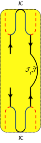
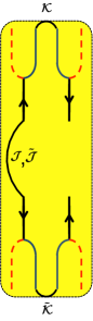
(a) (b) (c)

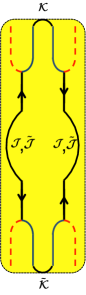
Figure 9: (Color online) The partial gapping of a single domino with local current-current interactions can be done in two ways (a) and (b). The complete gapping of a single domino with local current-current interactions is achieved in (c).

There is a crucial difference between either one of the boundary coset WZW theories with the central charge (118) and the chiral boundary theories from Sec. III.3. Starting from electrons, the latter can only be obtained on the one-dimensional boundaries of two-dimensional space. Starting from electrons, the former, however, can be obtained directly from either one of the strictly one-dimensional models represented by the single domino from Fig. 9(a) and the single domino from Fig. 9(b). For example, Fig. 9(a) realizes the same critical theory as the left boundary critical theory represented by Fig. 8 provided the interaction depicted in Fig. 9(a) that is defined by

$$\begin{split}\mathcal{L}^{\,}_{\mathrm{int}}:=&\,-\sum_{\mathcal{B}=1}^{3}\upsilon^{\mathcal{B}}_{\mathrm{boundary},1}\,\mathcal{K}^{\mathcal{B}}_{\mathrm{L},1}\,\mathcal{K}^{\mathcal{B}}_{\mathrm{R},1}\\ &\,-\sum_{\mathcal{A}=1}^{6}\lambda^{\mathcal{A}}_{\mathrm{boundary},1}\,\mathcal{J}^{\mathcal{A}}_{\mathrm{L},1}\,\widetilde{\mathcal{J}}^{\mathcal{A}}_{\mathrm{R},1}\\ &-\sum_{\mathcal{B}=1}^{3}\upsilon^{\mathcal{B}}_{\mathrm{boundary},1}\,\tilde{\mathcal{K}}^{\mathcal{B}}_{\mathrm{R},1}\,\tilde{\mathcal{K}}^{\mathcal{B}}_{\mathrm{L},1}\end{split}$$ (119)

preserves time-reversal symmetry. This is indeed the case as time reversal is represented by

$$\begin{split}&\mathcal{J}^{\mathcal{A}}_{\mathrm{L},1}\mapsto-\tilde{\mathcal{J}}^{\mathcal{A}}_{\mathrm{R},1},\qquad\mathcal{J}^{\mathcal{A}}_{\mathrm{R},1}\mapsto-\tilde{\mathcal{J}}^{\mathcal{A}}_{\mathrm{L},1},\\ &\tilde{\mathcal{J}}^{\mathcal{A}}_{\mathrm{R},1}\mapsto-\mathcal{J}^{\mathcal{A}}_{\mathrm{L},1},\qquad\tilde{\mathcal{J}}^{\mathcal{A}}_{\mathrm{L},1}\mapsto-\mathcal{J}^{\mathcal{A}}_{\mathrm{R},1},\\ &\mathcal{K}^{\mathcal{A}}_{\mathrm{L},1}\mapsto-\tilde{\mathcal{K}}^{\mathcal{A}}_{\mathrm{R},1},\qquad\mathcal{K}^{\mathcal{A}}_{\mathrm{R},1}\mapsto-\tilde{\mathcal{K}}^{\mathcal{A}}_{\mathrm{L},1},\\ &\tilde{\mathcal{K}}^{\mathcal{A}}_{\mathrm{R},1}\mapsto-\mathcal{K}^{\mathcal{A}}_{\mathrm{L},1},\qquad\tilde{\mathcal{K}}^{\mathcal{A}}_{\mathrm{L},1}\mapsto-\mathcal{K}^{\mathcal{A}}_{\mathrm{R},1},\end{split}$$ (120)

for $\mathcal{A}=1,\cdots,6$ and $\mathcal{B}=1,\cdots,3$. We emphasize that the transformation law (120) squares to unity.

On the one hand, it is shown in Appendix D that the time-reversal symmetry alone does not prevent gapping either one of the boundary coset WZW theories with the central charge (118) through one-body mass terms for the electrons. On the other hand, it is shown in Appendix D that the time-reversal symmetry together with the $U(1)$ symmetry under the linear transformation

$$\psi^{*}_{\mathrm{R}}\mapsto\psi^{*}_{\mathrm{R}}\,e^{-\mathrm{i}\theta},\qquad \tilde{\psi}^{*}_{\mathrm{R}}\mapsto\tilde{\psi}^{*}_{\mathrm{R}}\,e^{+\mathrm{i}\theta},$$ (121a)

$$\psi^{*}_{\mathrm{L}}\mapsto\psi^{*}_{\mathrm{L}}\,e^{-\mathrm{i}\theta},\qquad \tilde{\psi}^{*}_{\mathrm{L}}\mapsto\tilde{\psi}^{*}_{\mathrm{L}}\,e^{+\mathrm{i}\theta},$$ (121b)

$$\psi^{\,}_{\mathrm{R}}\mapsto e^{+\mathrm{i}\theta}\,\psi^{\,}_{\mathrm{R}},\qquad \tilde{\psi}^{\,}_{\mathrm{R}}\mapsto e^{-\mathrm{i}\theta}\,\tilde{\psi}^{\,}_{\mathrm{R}},$$ (121c)

$$\psi^{\,}_{\mathrm{L}}\mapsto e^{+\mathrm{i}\theta}\,\psi^{\,}_{\mathrm{L}}, \qquad\tilde{\psi}^{\,}_{\mathrm{L}}\mapsto e^{-\mathrm{i}\theta}\,\tilde{\psi}^{\,}_{\mathrm{L}},$$ (121d)

that is parameterized by $0\leq\theta<2\pi$, does prevent gapping through one-body mass terms for the electrons. Observe here that the $U(1)$ symmetry (121) of the Lagrangian densities (108), (116), and (119) is generated from the Ising-like linear transformation with the fundamental rules

$$\psi^{*}_{\mathrm{R}}\mapsto+\psi^{*}_{\mathrm{R}},\qquad \tilde{\psi}^{*}_{\mathrm{R}}\mapsto-\tilde{\psi}^{*}_{\mathrm{R}},$$ (122a)

$$\psi^{*}_{\mathrm{L}}\mapsto+\psi^{*}_{\mathrm{L}},\qquad \tilde{\psi}^{*}_{\mathrm{L}}\mapsto-\tilde{\psi}^{*}_{\mathrm{L}},$$ (122b)

$$\psi^{\,}_{\mathrm{R}}\mapsto+\psi^{\,}_{\mathrm{R}},\qquad \tilde{\psi}^{\,}_{\mathrm{R}}\mapsto-\tilde{\psi}^{\,}_{\mathrm{R}},$$ (122c)

$$\psi^{\,}_{\mathrm{L}}\mapsto+\psi^{\,}_{\mathrm{L}},\qquad \tilde{\psi}^{\,}_{\mathrm{L}}\mapsto-\tilde{\psi}^{\,}_{\mathrm{L}}.$$ (122d)

The $U(1)$ symmetry (121) is the analogue to the residual $U(1)$ spin-1/2 symmetry in the spin quantum Hall effect that insures the quantization of the spin Hall conductivity.   Kane and Mele (2005); Bernevig and Zhang (2006)

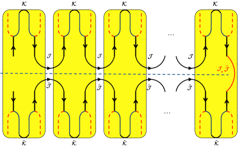
Figure 10: (Color online) Unfolding a chain of dominoes coupled by time-reversal symmetric interactions.

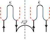
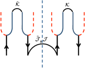
(a) (b) (c)

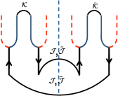
Figure 11: (Color online) The partial gapping of a bundle made of $2(k+k^{\prime})$ quantum wires with local current-current interactions can be done in two ways (a) and (b). The complete gapping of a bundle made of $2(k+k^{\prime})$ quantum wires with local current-current interactions is achieved in (c). The dashed vertical line is a mirror axis of symmetry.

However, as is implied by Fig. 9, it is possible to gap independently the coset theory with the central charge (118) on any one of the boundary at $\mathtt{m}=1$ and $\mathtt{m}=n$ by adding either the interaction

$$-\sum_{\mathcal{A}=1}^{6}\lambda^{\prime\mathcal{A}}_{\mathrm{boundary},1}\,\mathcal{J}^{\mathcal{A}}_{\mathrm{R},1}\,\widetilde{\mathcal{J}}^{\mathcal{A}}_{\mathrm{L},1}$$ (123)

(with $\lambda^{\prime\mathcal{A}}_{\mathrm{boundary},1}>0$) or the interaction

$$-\sum_{\mathcal{A}=1}^{6}\lambda^{\prime\mathcal{A}}_{\mathrm{boundary},\texttt{m}}\,\mathcal{J}^{\mathcal{A}}_{\mathrm{L},n}\,\widetilde{\mathcal{J}}^{\mathcal{A}}_{\mathrm{R},n}$$ (124)

(with $\lambda^{\prime\mathcal{A}}_{\mathrm{boundary},\texttt{m}}>0$), respectively. The transformation (121) acts trivially on the currents (84), (113), etc. Hence, imposing the symmetry under the transformation (121) is no rescue to prevent the instability of the helical edge states to local current-current interactions, as it was with regard to electronic mass terms.

The instability of the boundary states in Fig. 8 is not surprising. The low-energy sector of the theory after gapping the sectors with the $U(k+k^{\prime})$ and $\tilde{U}(k+k^{\prime})$ symmetries is of bosonic character, for it is solely expressed in terms of spin-1/2 currents. Time-reversal in this sector of the conformal embedding is represented by an operator that squares to the identity. If so, time-reversal symmetry is not expected to protect gapless boundary states. The existence of gapless boundary states demands fine-tuning of all strong many-body electronic interactions permitted by time-reversal symmetry.

This is not to say that the bulk theory in Fig. 8 is uninteresting. It does support topological order when two-dimensional space shares the same topology as that of a torus. When the ground state in Fig. 8 is the direct product of the ground state corresponding to Fig. 5(c) with its time-reversed image, the ground state corresponding to Fig. 5(d), the topological degeneracy is the square of the topological degeneracy corresponding to Fig. 5(c). This counting can be established as follows. We opt to gap the right-boundary in Fig. 8 as is illustrated in Fig. 10 with the vertical (red) arc. [We are caping the right boundary with Fig. 9(a).] We may then unfold the dominoes by cutting them about the dashed blue line in Fig. 10. The upper and lower parts of all dominoes are now interpreted to be distinct (by the presence of absence of the symbol $\tilde{\vphantom{A}}\$) quantum wires. We then recover Fig. 5(c) with $N$ replaced by $2N$. The operation of time-reversal is to be interpreted as a mirror transformation about the dashed line (i.e., non-local in space) after unfolding. We also observe that if we unfold the dominoes of Figs. 9(a), 9(b), and 9(c), we obtain the bundles made of $2(k+k^{\prime})$ quantum wires shown in Figs. 11(a), 11(b), and 11(c), respectively. Either of Figs. 11(a) and 11(b) realize a strongly interacting critical point of $2(k+k^{\prime})$ quantum wires obtained by fine-tuning of strong many-body electron interactions. This is reminiscent of the Takhtajan-Babujian critical point in the spin-1 chain with (competing) bilinear and biquadratic interactions,  Takhtajan (1982); Babujian (1982); Haldane (1983a, b); Affleck et al. (1987); Tsvelik (1990); Chubukov (1991); Kitazawa and Nomura (1999); Ivanov and Kolezhuk (2003); Liu et al. (2012); Lahtinen et al. (2014); Chen (2015) as well as of diverse spin-ladder systems with competing interactions.  Shelton et al. (1996); White and Affleck (1996); Nersesyan et al. (1998); Allen and Sénéchal (1997, 2000); Konik et al. (2010); Tsvelik (2011); Lecheminant and Nonne (2012); Lecheminant and Tsvelik (2015)

Even if open boundary conditions are imposed on two-dimensional space (two-dimensional space is the two-dimensional Euclidean plane) at infinity, “holes” in two-dimensional space bring about a topological degeneracy.  Iadecola et al. (2014) A “Hole” is here understood to be a path-connected and large region of two-dimensional space in which electrons are precluded from entering as is illustrated in Fig. 12 within the context of modeling two-dimensional space with a one-dimensional array of quantum wires. Electrons can neither tunnel nor interact with electrons across a large hole because of locality.

Figure 12: A single “hole” in a one-dimensional array of $N$ quantum wires. Electron tunneling between consecutive wires is prohibited across the diameter of the hole.

III.4.3 Case III – Broken rotation symmetry

The final example with time-reversal symmetry starts from a chain of decoupled and noninteracting wires that obeys time-reversal symmetry but with strongly broken spin-1/2 rotation symmetry. Instead of the low-energy theory (62) with its $SU(2)$ spin-1/2 rotation symmetry, we consider the case for which this symmetry is strongly broken down to no more than the $U(1)$ subgroup encoding rotations about a quantization axis. In this case, the non-Abelian spin-1/2 current algebra is no longer available to gap the bulk with current-current interactions. One must rely exclusively on the $SU(k)\times SU(k^{\prime})$ sector to gap the bulk with current-current interactions.

The construction of III.3 followed by those of Sec. III.4.1 and III.4.2 can then be reproduced if the spin-1/2 $SU(2)$ symmetry group is replaced by another $SU(2)$. To this end, we choose a bundle with $k=2l$ and $k^{\prime}=2l^{\prime}$ wires, where $l$ and $l^{\prime}$ are positive integers. We then use the direct-product decomposition $U(2k)\times U(2k^{\prime})$, where any one the two unitary groups is decomposed according to the rule $U(2k)=U(4l)=U(1)\times SU(4l)$ and similarly for $k\to k^{\prime}$. We impose on $SU(4l)$ the conformal embedding corresponding to $SU(2)\times SU(2)\times SU(l)$, where the first $SU(2)$ is generated by the spin-1/2 of the electron. By assumption, this sector is strongly gapped. Thus, we may ignore it in the low-energy sector of the theory. We then proceed with the sectors $U(1)\times SU(2)\times SU(l)$ as we did in Secs. III.3 and Sec. III.4.1. To duplicate III.4.2, we furthermore introduce the doubling $\widetilde{SU}(2)$ that we may interpret as assuming that $l=2o$ and $l^{\prime}=2o^{\prime}$ with $o$ and $o^{\prime}$ positive integers.

Finally, we observe one can also use the $U(1)$ charge sector or the $U(1)$ sector for rotations about the spin-1/2 quantization axis to gap the bulk while leaving gapless boundaries.   Bernevig and Zhang (2006); Levin and Stern (2009); Neupert et al. (2011); Levin and Stern (2012)

Appendix A Reversal of time

A.1 Complex fermions

A.1.1 Spinless case

Denote the fermion annihilation and creation field operators as $\hat{\psi}^{{\dagger}}_{\mathrm{A}}(t,x)$ and $\hat{\psi}^{\,}_{\mathrm{A}}(t,x)$, respectively. The index $\mathrm{A}$ belongs to a countable set. A point in time is denoted by $t$. A point in space is denoted by $x$. The only nonvanishing equal-time anticommutators are

$$\left\{\hat{\psi}^{\,}_{\mathrm{A}}(t,x),\hat{\psi}^{{\dagger}}_{\mathrm{A}^{\prime}}(t,x^{\prime})\right\}=\delta^{\,}_{\mathrm{A}\mathrm{A}^{\prime}}\,\delta(x-x^{\prime}).$$ (125a)

For the spinless case,

$$\mathrm{A}=\mathrm{R},\mathrm{L},$$ (125b)

i.e., the collective index $\mathrm{A}$ takes the value $\mathrm{R}$ and $\mathrm{L}$ with “$\mathrm{R}$” standing for a right mover and “$\mathrm{L}$” standing for a left mover.

Reversal of time is the antilinear transformation on the $*$-algebra generated by the quantum fields (125) with the fundamental rule

$$\hat{\psi}^{\,}_{\mathrm{R}}(t,x)\mapsto\hat{\psi}^{\,}_{\mathrm{L}}(-t,x),\qquad\hat{\psi}^{\,}_{\mathrm{L}}(t,x)\mapsto\hat{\psi}^{\,}_{\mathrm{R}}(-t,x).$$ (126)

Exchange of particle and hole is the linear transformation on the $*$-algebra generated by the quantum fields (125) with the fundamental rule

$$\hat{\psi}^{\,}_{\mathrm{R}}(t,x)\mapsto\hat{\psi}^{{\dagger}}_{\mathrm{R}}(t,x),\qquad\hat{\psi}^{\,}_{\mathrm{L}}(t,x)\mapsto\hat{\psi}^{{\dagger}}_{\mathrm{L}}(t,x).$$ (127)

A.1.2 Spin-1/2 case

Denote the spin-$1/2$ Dirac field operator as $\hat{\psi}^{\,}_{\mathrm{A}}(t,x)$. The index $\mathrm{A}$ belongs to a countable set. A point in time is denoted by $t$. A point in space is denoted by $x$. The only nonvanishing equal-time anticommutators are

$$\left\{\hat{\psi}^{\,}_{\mathrm{A}}(t,x),\hat{\psi}^{{\dagger}}_{\mathrm{A}^{\prime}}(t,x^{\prime})\right\}=\delta^{\,}_{\mathrm{A}\mathrm{A}^{\prime}}\,\delta(x-x^{\prime}).$$ (128a)

For the spin-$$1/2$$ case,

$$\mathrm{A}=(\mathrm{R},+),(\mathrm{R},-),(\mathrm{L},+),(\mathrm{L},-),$$ (128b)

i.e., the collective index $\mathrm{A}$ enumerates right and left movers with an helicity index $\sigma=\pm$ that can be interpreted as the projection of a spin-$1/2$ quantum number along the Fermi wave vector.

Reversal of time is the antilinear transformation on the $*$-algebra generated by the quantum fields (128) with the fundamental rule

$$\begin{split}&\hat{\psi}^{\,}_{\mathrm{R},+}(t,x)\mapsto+\hat{\psi}^{\,}_{\mathrm{L},-}(-t,x),\\ &\hat{\psi}^{\,}_{\mathrm{R},-}(t,x)\mapsto-\hat{\psi}^{\,}_{\mathrm{L},+}(-t,x),\\ &\hat{\psi}^{\,}_{\mathrm{L},+}(t,x)\mapsto+\hat{\psi}^{\,}_{\mathrm{R},-}(-t,x),\\ &\hat{\psi}^{\,}_{\mathrm{L},-}(t,x)\mapsto-\hat{\psi}^{\,}_{\mathrm{R},+}(-t,x).\end{split}$$ (129)

Exchange of particle and hole is the linear transformation on the $*$-algebra generated by the quantum fields (128) with the fundamental rule

$$\hat{\psi}^{\,}_{\mathrm{A}}(t,x)\mapsto\hat{\psi}^{{\dagger}}_{\mathrm{A}}(t,x)$$ (130)

for $\mathrm{A}=(R,+),(R,-),(L,+),(L,-)$.

A.2 Real Fermions

A.2.1 Spinless case

We start from the $*$-algebra defined from Eq. (125). We write

$$\hat{\psi}^{\,}_{\mathrm{A}}(t,x)\equiv\frac{1}{\sqrt{2}}\left[\hat{\chi}^{\,}_{\mathrm{A},1}(t,x)+\mathrm{i}\hat{\chi}^{\,}_{\mathrm{A},2}(t,x)\right]$$ (131a)

and demand that

$$\hat{\chi}^{{\dagger}}_{\mathrm{A},1}(t,x)=\hat{\chi}^{\,}_{\mathrm{A},1}(t,x),\qquad\hat{\chi}^{{\dagger}}_{\mathrm{A},2}(t,x)=\hat{\chi}^{\,}_{\mathrm{A},2}(t,x),$$ (131b)

holds together with the equal-time algebra

$$\left\{\hat{\chi}^{\,}_{\mathrm{A},a}(t,x),\hat{\chi}^{\,}_{\mathrm{A}^{\prime},a^{\prime}}(t,x^{\prime})\right\}=\delta^{\,}_{\mathrm{A}\mathrm{A}^{\prime}}\,\delta^{\,}_{aa^{\prime}}\,\delta(x-x^{\prime}),$$ (131c)

for $\mathrm{A},\mathrm{A}^{\prime}=\mathrm{R},\mathrm{L}$ and $a,a^{\prime}=1,2$.

Reversal of time is the antilinear transformation on the $*$-algebra generated by the quantum fields (131) with the fundamental rule

$$\begin{split}&\hat{\chi}^{\,}_{\mathrm{R},a}(t,x)\mapsto(-1)^{a-1}\,\hat{\chi}^{\,}_{\mathrm{L},a}(-t,x),\\ &\hat{\chi}^{\,}_{\mathrm{L},a}(t,x)\mapsto(-1)^{a-1}\,\hat{\chi}^{\,}_{\mathrm{R},a}(-t,x),\end{split}$$ (132)

for $a=1,2$. The multiplicative negative sign when $a=2$ arises because of the antilinearity. Here, reversal of time squares to the identity.

Exchange of particle and hole is the linear transformation on the $*$-algebra generated by the quantum fields (131) with the fundamental rule

$$\hat{\chi}^{\,}_{\mathrm{A},1}(t,x)\mapsto\hat{\chi}^{\,}_{\mathrm{A},1}(t,x),\qquad\hat{\chi}^{\,}_{\mathrm{A},2}(t,x)\mapsto-\hat{\chi}^{\,}_{\mathrm{A},2}(t,x),$$ (133)

for $\mathrm{A}=\mathrm{R},\mathrm{L}$. Exchange of particle and hole squares to the identity here.

A.2.2 Spin-1/2 case

We start from $*$-algebra defined from Eq. (128). We write

$$\hat{\psi}^{\,}_{\mathrm{A}}(t,x)\equiv\frac{1}{\sqrt{2}}\left[\hat{\chi}^{\,}_{\mathrm{A},1}(t,x)+\mathrm{i}\hat{\chi}^{\,}_{\mathrm{A},2}(t,x)\right]$$ (134a)

and demand that

$$\hat{\chi}^{{\dagger}}_{\mathrm{A},1}(t,x)=\hat{\chi}^{\,}_{\mathrm{A},1}(t,x),\qquad\hat{\chi}^{{\dagger}}_{\mathrm{A},2}(t,x)=\hat{\chi}^{\,}_{\mathrm{A},2}(t,x),$$ (134b)

holds together with the equal-time algebra

$$\left\{\hat{\chi}^{\,}_{\mathrm{A},a}(t,x),\hat{\chi}^{\,}_{\mathrm{A}^{\prime},a^{\prime}}(t,x^{\prime})\right\}=\delta^{\,}_{\mathrm{A}\mathrm{A}^{\prime}}\,\delta^{\,}_{aa^{\prime}}\,\delta(x-x^{\prime}),$$ (134c)

for $\mathrm{A},\mathrm{A}^{\prime}=(\mathrm{R},+),(\mathrm{R},-),(\mathrm{L},+),(\mathrm{L},-)$ and $a,a^{\prime}=1,2$.

Reversal of time is the antilinear transformation on the $*$-algebra generated by the quantum fields (134) with the fundamental rule

$$\begin{split}&\hat{\chi}^{\,}_{\mathrm{R},+,a}(t,x)\mapsto+(-1)^{a-1}\,\hat{\chi}^{\,}_{\mathrm{L},-,a}(-t,x),\\ &\hat{\chi}^{\,}_{\mathrm{R},-,a}(t,x)\mapsto-(-1)^{a-1}\,\hat{\chi}^{\,}_{\mathrm{L},+,a}(-t,x),\\ &\hat{\chi}^{\,}_{\mathrm{L},+,a}(t,x)\mapsto+(-1)^{a-1}\,\hat{\chi}^{\,}_{\mathrm{R},-,a}(-t,x),\\ &\hat{\chi}^{\,}_{\mathrm{L},-,a}(t,x)\mapsto-(-1)^{a-1}\,\hat{\chi}^{\,}_{\mathrm{R},+,a}(-t,x),\end{split}$$ (135)

for $a=1,2$. Here, reversal of time squares to minus the identity.

Exchange of particle and hole can be implemented in two ways.

One may choose the linear transformation on the $*$-algebra generated by the quantum fields (134) with the fundamental rule

$$\begin{split}&\hat{\chi}^{\,}_{\mathrm{A},a}(t,x)\mapsto(-1)^{a-1}\,\hat{\chi}^{\,}_{\mathrm{A},a}(t,x)\end{split}$$ (136)

for $\mathrm{A}=(\mathrm{R},+),(\mathrm{R},-),(\mathrm{L},+),(\mathrm{L},-)$ and $a=1,2$. This transformation squares to the identity.

One may choose the linear transformation on the $*$-algebra generated by the quantum fields (134) with the fundamental rule

$$\begin{split}&\hat{\chi}^{\,}_{\alpha,+,a}(t,x)\mapsto(-1)^{a-1}\,\hat{\chi}^{\,}_{\alpha,-,a}(t,x),\\ &\hat{\chi}^{\,}_{\alpha,-,a}(t,x)\mapsto-(-1)^{a-1}\,\hat{\chi}^{\,}_{\alpha,+,a}(t,x),\end{split}$$ (137)

for $\alpha=\mathrm{R},\mathrm{L}$ and $a=1,2$. This transformation squares to minus the identity.

Appendix B Non-Abelian bosonization for the symmetry classes C, A, and AII

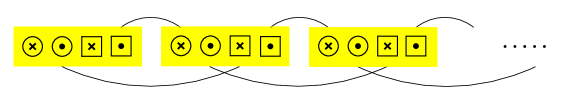
Figure 13: (Color online) Pictorial representation for the selected backscattering in the symmetry class C. Each yellow box represents a quantum wire composed of four-Majorana degrees of freedom. The wires are enumerated by $I=1,\cdots,N$ in ascending order from left to right. For any $I$, the Majorana modes are denoted by $\chi^{\,}_{\mathrm{R},+,I}$, $\chi^{\,}_{\mathrm{L},+,I}$, $\chi^{\,}_{\mathrm{R},-,I}$, and $\chi^{\,}_{\mathrm{L},-,I}$ reading from left to right, respectively.

B.1 The symmetry class C

The simplest model for an array of quantum wires in the symmetry class C to realize a topological gapped phase is defined in two steps. First, the superscript (DIII) is replaced by (C) in Eq. (50). Second, we impose the linear transformation defined by the fundamental rule

$$\begin{split}&\chi^{\,}_{\mathrm{R},+,I}(t,x)\mapsto+\,\chi^{\,}_{\mathrm{R},-,I}(t,x),\\ &\chi^{\,}_{\mathrm{R},-,I}(t,x)\mapsto-\,\chi^{\,}_{\mathrm{R},+,I}(t,x),\\ &\chi^{\,}_{\mathrm{L},+,I}(t,x)\mapsto+\,\chi^{\,}_{\mathrm{L},-,I}(t,x),\\ &\chi^{\,}_{\mathrm{L},-,I}(t,x)\mapsto-\,\chi^{\,}_{\mathrm{L},+,I}(t,x),\end{split}$$ (138)

for $I=1,\cdots,N$.  Altland and Zirnbauer (1997) Transformation (138) squares to minus the identity. Even though reversal of time (51c) is a symmetry of the partition function $Z^{(\mathrm{C})}_{0}$, we shall not impose invariance under reversal of time (51c) for a generic representative of the symmetry class C.

Any partition function $Z^{(\mathrm{C})}$ for the array of quantum wires is said to belong to the symmetry class C if $Z^{(\mathrm{C})}$ is invariant under the following transformations. There is the symmetry (138). There is the symmetry under the linear transformation (fermion parity) with the fundamental rule

$$\chi^{\,}_{\alpha,\mathrm{f},I}\mapsto-\chi^{\,}_{\alpha,\mathrm{f},I}$$ (139)

for any $\alpha=\mathrm{R},\mathrm{L}$, $\mathrm{f}=\pm$, and $I=1,\cdots,N$. Both symmetries generate the symmetry under the linear $O(2)$ transformation

$$\chi^{\,}_{\alpha,\mathrm{f},I}\mapsto O^{\,}_{\mathrm{f}\mathrm{f}^{\prime}}\,\chi^{\,}_{\alpha,\mathrm{f}^{\prime},I}$$ (140)

for any $\alpha=\mathrm{R},\mathrm{L}$, $\mathrm{f}=\pm$, and $I=1,\cdots,N$. Here, the summation convention over the repeated indices $\mathrm{f}^{\prime}=\pm$ is implied and the $2\times 2$ matrix $(O^{\,}_{\mathrm{f}\mathrm{f}^{\prime}})$ is real-valued and orthogonal.

We seek a local single-particle perturbation $\mathcal{L}^{(\mathrm{C})}_{\mathrm{mass}}$ that satisfies three conditions when added to the Lagrangian density $\mathcal{L}^{(\mathrm{C})}_{0}$.

Condition C.1 It must be invariant under the transformations (138) and (139).

Condition C.2 It must gap completely the theory with the partition function $Z^{(\mathrm{C})}_{0}$ if we impose the periodic boundary conditions

$$\chi^{\,}_{\alpha,\mathrm{f},I}(t,x)=\chi^{\,}_{\alpha,\mathrm{f},I+N}(t,x)$$ (141)

for $\alpha=\mathrm{R},\mathrm{L}$, $\mathrm{f}=\pm$, and $I=1,\cdots,N$.

Condition C.3 The partition function $Z^{(\mathrm{C})}$ with the Lagrangian density $\mathcal{L}^{(\mathrm{C})}_{0}+\mathcal{L}^{(\mathrm{C})}_{\mathrm{mass}}$ must be a theory with the central charge

$$c^{(\mathrm{C})}=1$$ (142)

if open boundary condition are imposed.

Conditions C.1, C.2, and C.3 imply that we may assign wire $I=1$ the right-chiral central charge $1$ and wire $I=N$ the left-chiral central charge $1$, for wires $I=1$ and $I=N$ both support a degenerate pair of right- or left-moving Majorana edge modes, respectively.

We make the Ansatz

$$\mathcal{L}^{(\mathrm{C})}_{\mathrm{mass}}:=\sum_{I=1}^{N-1}\mathrm{i}\lambda\,\left(\chi^{\,}_{\mathrm{L},-,I}\,\chi^{\,}_{\mathrm{R},+,I+1}-\chi^{\,}_{\mathrm{L},+,I}\,\chi^{\,}_{\mathrm{R},-,I+1}\right)$$ (143)

with $\lambda$ a real-valued coupling. Condition C.1 is met by construction. To establish that the Ansatz (143) meets Conditions C.2 and C.3, we use non-Abelian bosonization. We choose the non-Abelian bosonization scheme by which the partition function is given by the path integral

$$Z^{(\mathrm{C})}=\int\mathcal{D}[G]\,e^{\mathrm{i}S^{(\mathrm{C})}}.$$ (144a)

The field $$G\in O(2N) \mathcal{D}[G] O(2N) S^{(\mathrm{C})} S^{(\mathrm{C})}_{0} S^{(\mathrm{C})}_{\mathrm{mass}} S^{(\mathrm{C})}_{0}$$ is a matrix of bosons. The measure is constructed from the Haar measure on . The action is the sum of the actions and . The action is

$$\begin{split}S^{(\mathrm{C})}_{0}=&\,\frac{1}{16\pi}\int\mathrm{d}t\int\mathrm{d}x\,\mathrm{tr}\,\left(\partial^{\,}_{\mu}G\,\partial^{\mu}G^{-1}\right)\\ &\,+\frac{1}{24\pi}\int\limits_{B}\mathrm{d}^{3}y\,\mathcal{L}^{(\mathrm{C})}_{\mathrm{WZW}},\end{split}$$ (144b)

where

$$\mathcal{L}^{(\mathrm{C})}_{\mathrm{WZW}}=\epsilon^{ijk}\,\mathrm{tr}\,\Bigl{[}(\bar{G}^{-1}\partial^{\,}_{i}\bar{G})\,(\bar{G}^{-1}\partial^{\,}_{j}\bar{G})(\bar{G}^{-1}\partial^{\,}_{k}\bar{G})\Bigr{]}.$$ (144c)

(Recall that $$\bar{G} G S^{(\mathrm{C})}_{\mathrm{mass}}$$ denotes the extension of to the solid 3-ball.) The action stems from the Lagrangian density

$$\begin{split}\mathcal{L}^{(\mathrm{C})}_{\mathrm{mass}}=&\,\sum_{I=1}^{N-1}\lambda\,\left(G^{\,}_{(-,I),(-,I+1)}+G^{\,}_{(+,I+1),(+,I)}\right)\\ \equiv&\,\lambda\,\mathrm{tr}\,\left(M^{(\mathrm{C})}\,G\right).\end{split}$$ (144d)

The second equality is established by using the non-Abelian bosonization formula (30) (we have set the mass parameter $$m^{\,}_{\mathrm{uv}}=1 2N\times 2N M^{(\mathrm{C})}$$). The matrices is represented by

$$M^{(\mathrm{C})}:=\begin{pmatrix}0&0&0&0&0&0&\cdots\\ B&0&0&0&0&0&\cdots\\ 0&B&0&0&0&0&\cdots\\ 0&0&B&0&0&0&\cdots\\ 0&0&0&B&0&0&\cdots\\ 0&0&0&0&B&0&\cdots\\ \vdots&\vdots&\vdots&\vdots&\vdots&\vdots&\ddots\\ \end{pmatrix}$$ (144e)

in the basis for which $$B 2\times 2$$ is the matrix

$$B:=\begin{pmatrix}\overbrace{-1}^{(-,+)}&\overbrace{0}^{(-,-)}\\ \underbrace{0}_{(+,+)}&\underbrace{1}_{(+,-)}\end{pmatrix}.$$ (144f)

For any $N>2$, the $2N\times 2N$ matrices $M^{(\mathrm{C})}$ defined by (144e) has two vanishing and $2\times(N-1)$ nonvanishing eigenvalues.

The quadratic perturbation (144d) thus reduces the central charge $c^{(\mathrm{C})}_{0}=2\times N/2$ by the amount $2\times(N-1)/2$, i.e., the central charge for the theory with the partition function $Z^{(\mathrm{C})}$ is

$$c^{(\mathrm{C})}=\frac{2\times N}{2}-\frac{2\times(N-1)}{2}=1.$$ (145)

We have constructed a topological superconductor with the gapless and singlet pair of Majorana modes $(\chi^{\,}_{\mathrm{R},+,I},\chi^{\,}_{\mathrm{R},-,I})^{\,}_{I=1}$ propagating along edge $I=1$ and the gapless and singlet pair of Majorana modes $(\chi^{\,}_{\mathrm{L},+,I},\chi^{\,}_{\mathrm{L},-,I})^{\,}_{I=N}$ propagating along edge $I=N$. This construction is summarized by Fig. 13.

The symmetry class C has the $\mathbb{Z}$ topological classification for the following reason. If one takes an arbitrary integer number $\nu$ of copies of the gapless edge theory, these $\nu$-copies remain gapless. The stability of the $2\nu$ gapless edge modes within either wire 1 or wire $N$ is guaranteed because backscattering among gapless chiral edges modes of the same chirality is not allowed kinematically within either wire 1 or wire $N$.

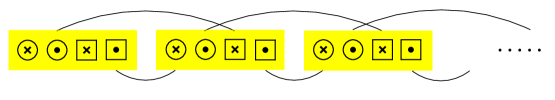
Figure 14: (Color online) Pictorial representation for the selected backscattering in the symmetry class A. Each yellow box represents a quantum wire composed of four-Majorana degrees of freedom. The wires are enumerated by $I=1,\cdots,N$ in ascending order from left to right. For any $I$, the Majorana modes are denoted by $\chi^{\,}_{\mathrm{R},1,I}$, $\chi^{\,}_{\mathrm{L},1,I}$, $\chi^{\,}_{\mathrm{R},2,I}$, and $\chi^{\,}_{\mathrm{L},2,I}$ reading from left to right, respectively.

B.2 The symmetry class A

The symmetry class A preserves the total number of complex fermions that can be built out of an even number $M$ of flavors for the Majorana fermions. The simplest model for an array of quantum wires in the symmetry class A to realize a topological gapped phase assumes

$$M=2,\qquad\chi^{\,}_{\alpha,\mathrm{f},I}(t,x),$$ (146a)

for $$\alpha=\mathrm{R},\mathrm{L} \mathrm{f}=1,2 I=1,\cdots,N I=1\,\cdots\,N$$, , and . We have thus assigned four Majorana fermions to each wire . If so, we can interpret

$$\begin{split}&\psi^{*}_{\alpha,I}(t,x)\equiv\frac{1}{\sqrt{2}}\left[{\chi}^{\,}_{\alpha,1,I}(t,x)-\mathrm{i}{\chi}^{\,}_{\alpha,2,I}(t,x)\right],\\ &\psi^{\,}_{\alpha,I}(t,x)\equiv\frac{1}{\sqrt{2}}\left[{\chi}^{\,}_{\alpha,1,I}(t,x)+\mathrm{i}{\chi}^{\,}_{\alpha,2,I}(t,x)\right],\end{split}$$ (146b)

for $\alpha=\mathrm{R},\mathrm{L}$ and $I=1,\cdots,N$ as the Grassmann representation of a pair of creation and annihilation fermion operators.

The simplest model for an array of quantum wires in the symmetry class A to realize a topological gapped phase is defined in two steps. First, the superscript (DIII) is replaced by (A) in Eq. (50). There follows the partition function $Z^{(\mathrm{A})}_{0}$. Second, we shall represent reversal of time with the antilinear transformation defined by the fundamental rule [see Eq. (132)]

$$\begin{split}&\chi^{\,}_{\mathrm{R},\mathrm{f},I}(t,x)\mapsto(-1)^{\mathrm{f}-1}\,\chi^{\,}_{\mathrm{L},\mathrm{f},I}(-t,x),\\ &\chi^{\,}_{\mathrm{L},\mathrm{f},I}(t,x)\mapsto(-1)^{\mathrm{f}-1}\,\chi^{\,}_{\mathrm{R},\mathrm{f},I}(-t,x),\end{split}$$ (147)

for $\mathrm{f}=1,2$ and $I=1,\cdots,N$. Contrary to the reversal of time defined by Eq. (51c), transformation (147) squares to the identity. Even though reversal of time (147) is a symmetry of the partition function $Z^{(\mathrm{A})}_{0}$, we shall not impose invariance under reversal of time (147) for a generic representative of the symmetry class A. A symmetry of the partition function $Z^{(\mathrm{A})}_{0}$ that we shall keep is the $O(2)$ symmetry under the transformation (148b) that is parametrized by the angle $0\leq\theta<2\pi$.

The theory with the partition function $Z^{(A)}_{0}$ is critical, for there are $4N$ decoupled massless Majorana modes that are dispersing in $(1+1)$-dimensional Minkowski space and time. Hence, the central charge for the partition function $Z^{(\mathrm{A})}_{0}$ is

$$c^{(\mathrm{A})}_{0}=N.$$ (148a)

The partition function $$Z^{(\mathrm{A})}_{0} O^{\,}_{\mathrm{R}}(2N)\times O^{\,}_{L}(2N) 0\leq\theta<2\pi Z^{(\mathrm{A})}_{0}$$ is invariant under any local linear transformation from of the form (51b). For any , is also invariant under the continuous global linear transformation with the fundamental rule

$$\begin{split}&\chi^{\,}_{\alpha,1,I}(t,x)\mapsto\cos\theta\,\chi^{\,}_{\alpha,1,I}(t,x)-\sin\theta\,\chi^{\,}_{\alpha,2,I}(t,x),\\ &\chi^{\,}_{\alpha,2,I}(t,x)\mapsto\sin\theta\,\chi^{\,}_{\alpha,1,I}(t,x)+\cos\theta\,\chi^{\,}_{\alpha,2,I}(t,x),\end{split}$$ (148b)

for $$\alpha=\mathrm{R},\mathrm{L} I=1,\cdots,N U(1) U(1)$$ and . This transformation implements the fermion-number conservation law that follows from the symmetry under the global transformation

$$\begin{split}&\psi^{*}_{\alpha,I}(t,x)\mapsto\psi^{*}_{\alpha,I}(t,x)\,e^{-\mathrm{i}\theta}\\ &\psi^{\,}_{\alpha,I}(t,x)\mapsto e^{+\mathrm{i}\theta}\,\psi^{\,}_{\alpha,I}(t,x),\end{split}$$ (148c)

for any $0\leq\theta<2\pi$, $\alpha=\mathrm{R},\mathrm{L}$, and $I=1,\cdots,N$.

Any partition function $Z^{(\mathrm{A})}$ for the array of quantum wires is said to belong to the symmetry class A if $Z^{(\mathrm{A})}$ is invariant under the global linear $O(2)$ transformation (148b).

Even though the $O(2)$ symmetry in the simplest model for an array of quantum wires in the symmetry class A has a very different origin from that in the minimal model for an array of quantum wires in the symmetry class C, we may still borrow the analysis of Sec. B.1 below Eq. (140) verbatim. This construction of a topological phase in the symmetry class A is summarized by Fig. 14.

The symmetry class A has the $\mathbb{Z}$ topological classification for the following reason. If one takes an arbitrary integer number $\nu$ of copies of the gapless edge theory, these $\nu$-copies remain gapless. The stability of the $2\nu$ Majorana gapless edge modes within either wire 1 or wire $N$ is guaranteed for two reasons. First, the $O(2)$ conservation law allows to group two Majorana fermions into one complex chiral fermion. Second, all Majorana modes within either wire 1 or wire $N$ share the same chirality, backscattering among gapless edges modes is not allowed kinematically within either wire 1 or wire $N$.

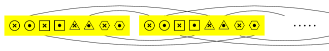
Figure 15: (Color online) Pictorial representation for the selected backscattering in the symmetry class AII. Each yellow box represents a quantum wire composed of four-Majorana degrees of freedom. The wires are enumerated by $I=1,\cdots,N$ in ascending order from left to right. For any $I$, the Majorana modes are denoted by $\chi^{\,}_{\mathrm{R},+,1,I}$, $\chi^{\,}_{\mathrm{L},+,1,I}$, $\chi^{\,}_{\mathrm{R},-,1,I}$, $\chi^{\,}_{\mathrm{L},-,1,I}$, $\chi^{\,}_{\mathrm{R},+,2,I}$, $\chi^{\,}_{\mathrm{L},+,2,I}$, $\chi^{\,}_{\mathrm{R},-,2,I}$, and $\chi^{\,}_{\mathrm{L},-,2,I}$ reading from left to right, respectively.

B.3 The symmetry class AII

Fermion-number conservation and a time-reversal symmetry squaring to minus the identity must hold in the symmetry class AII. The time-reversal symmetry is that of spin-$1/2$. The minimal model in the symmetry class AII for an array of quantum wires must thus accommodate twice as many degrees of freedom as that in the symmetry class A in order to realize a topological insulating phase.

The simplest model for an array of quantum wires in the symmetry class AII to realize a topological gapped phase assumes

$$M=4,\qquad\chi^{\,}_{\alpha,\sigma,a,I}(t,x),$$ (149a)

with the right- and left-mover labels $$\alpha=\mathrm{R},\mathrm{L} \sigma=\pm a=1,2, I=1,\cdots,N$$, the helicity labels , the complex fermion labels and the wire index . This is to say that four complex fermions are represented by

$${\psi}^{\,}_{A}(t,x)\equiv\frac{1}{\sqrt{2}}\left[{\chi}^{\,}_{A,1}(t,x)+\mathrm{i}{\chi}^{\,}_{A,2}(t,x)\right]$$ (149b)

with the collective label $$\mathrm{A}=(\mathrm{R},+),(\mathrm{R},-),(\mathrm{L},+),(\mathrm{L},-)$$. We define the action

$$S^{(\mathrm{AII})}_{0}:=\int\mathrm{d}t\int\mathrm{d}x\,\mathcal{L}^{(\mathrm{AII})}_{0}$$ (149c)

with

$$\begin{split}\mathcal{L}^{(\mathrm{AII})}_{0}:=&\,\frac{\mathrm{i}}{2}\sum_{I=1}^{N}\sum_{\sigma=\pm}\sum_{a=1,2}\Bigl{[}\chi^{\,}_{\mathrm{R},\sigma,a,I}\left(\partial^{\,}_{t}+\partial^{\,}_{x}\right)\chi^{\,}_{\mathrm{R},\sigma,a,I}\\ &\,+\chi^{\,}_{\mathrm{L},\sigma,a,I}\left(\partial^{\,}_{t}-\partial^{\,}_{x}\right)\chi^{\,}_{\mathrm{L},\sigma,a,I}\Bigr{]}.\end{split}$$ (149d)

We also define the Grassmann partition function

$$Z^{(\mathrm{AII})}_{0}:=\int\mathcal{D}[\chi]\,e^{+\mathrm{i}S^{(\mathrm{AII})}_{0}}.$$ (149e)

The theory with the partition function $Z^{(\mathrm{AII})}_{0}$ is critical, for there are $8N$ decoupled massless Majorana modes that are dispersing in $(1+1)$-dimensional Minkowski space and time. Hence, the central charge for the theory with the partition function $Z^{(\mathrm{AII})}_{0}$ is

$$c^{(\mathrm{AII})}_{0}=2N.$$ (150a)

The partition function $$Z^{(\mathrm{AII})}_{0} (O^{(\mathrm{R})},O^{(\mathrm{L})})\in O^{\,}_{\mathrm{R}}(4N)\times O^{\,}_{\mathrm{L}}(4N)$$ is invariant under any local transformation defined by

$$\begin{split}&\chi^{\,}_{\mathrm{R}}(t-x)\mapsto O^{(\mathrm{R})}(t-x)\,\chi^{\,}_{\mathrm{R}}(t-x),\\ &\chi^{\,}_{\mathrm{L}}(t+x)\mapsto O^{(\mathrm{L})}(t+x)\,\chi^{\,}_{\mathrm{L}}(t+x).\end{split}$$ (150b)

It is also invariant under the antilinear transformation with the fundamental rules

$$\begin{split}&\chi^{\,}_{\mathrm{R},+,a,I}(t,x)\mapsto+(-1)^{a-1}\,\chi^{\,}_{\mathrm{L},-,a,I}(-t,x),\\ &\chi^{\,}_{\mathrm{R},-,a,I}(t,x)\mapsto-(-1)^{a-1}\,\chi^{\,}_{\mathrm{L},+,a,I}(-t,x),\\ &\chi^{\,}_{\mathrm{L},+,a,I}(t,x)\mapsto+(-1)^{a-1}\,\chi^{\,}_{\mathrm{R},-,a,I}(-t,x),\\ &\chi^{\,}_{\mathrm{L},-,a,I}(t,x)\mapsto-(-1)^{a-1}\,\chi^{\,}_{\mathrm{R},+,a,I}(-t,x),\end{split}$$ (150c)

for $$a=1,2$$ that implement reversal of time in such a way that reversal of time squares to minus the identity (see Appendix A). Finally, it is invariant under the linear transformation with the fundamental rule

$$\begin{split}&\chi^{\,}_{\mathrm{A},1,I}(t,x)\mapsto\cos\theta\,\chi^{\,}_{\mathrm{A},1,I}(t,x)-\sin\theta\,\chi^{\,}_{\mathrm{A},2,I}(t,x),\\ &\chi^{\,}_{\mathrm{A},2,I}(t,x)\mapsto\sin\theta\,\chi^{\,}_{\mathrm{A},1,I}(t,x)+\cos\theta\,\chi^{\,}_{\mathrm{A},2,I}(t,x),\end{split}$$ (150d)

that implements the global $$U(1)$$ transformation

$$\begin{split}&\psi^{*}_{\mathrm{A},I}(t,x)\mapsto\psi^{*}_{\mathrm{A},I}(t,x)\,e^{-\mathrm{i}\theta},\\ &\psi^{\,}_{\mathrm{A},I}(t,x)\mapsto e^{+\mathrm{i}\theta}\,\psi^{\,}_{\mathrm{A},I}(t,x),\end{split}$$ (150e)

for $\mathrm{A}=(R,+),(R,-),(L,+),(L,-)$ and any $0\leq\theta<2\pi$.

Any partition function $Z^{(\mathrm{AII})}$ for the array of quantum wires is said to belong to the symmetry class AII if $Z^{(\mathrm{AII})}$ is invariant under the transformations (150c) and (150d).

We seek a local single-particle perturbation $\mathcal{L}^{(\mathrm{AII})}_{\mathrm{mass}}$ that satisfies three conditions when added to the Lagrangian density (149d).

Condition AII.1 It must be invariant under the transformations (150c) and (150d).

Condition AII.2 It must gap completely the theory with the partition function $Z^{(\mathrm{AII})}_{0}$ if we impose the periodic boundary conditions

$$\chi^{\,}_{\alpha,\mathrm{f},a,I}(t,x)=\chi^{\,}_{\alpha,\mathrm{f},a,I+N}(t,x)$$ (151)

for $\alpha=\mathrm{R},\mathrm{L}$, $\mathrm{f}=\pm$, $a=1,2$, and $I=1,\cdots,N$.

Condition AII.3 The partition function $Z^{(\mathrm{AII})}$ with the Lagrangian density $\mathcal{L}^{(\mathrm{AII})}_{0}+\mathcal{L}^{(\mathrm{AII})}_{\mathrm{mass}}$ must be a theory with the central charge

$$c^{(\mathrm{AII})}=2$$ (152)

if open boundary condition are imposed.

Conditions AII.1, AII.2, and AII.3 imply that we may assign wire $I=1$ the central charge $1$ and wire $I=N$ the central charge $1$, for wires $I=1$ and $I=N$ both support a single Kramers degenerate pair of edge modes, whereby each mode carries the sharp (complex) fermion number of one.

We make the Ansatz

$$\begin{split}\mathcal{L}^{(\mathrm{AII})}_{\mathrm{mass}}:=&\,\sum_{I=1}^{N-1}\mathrm{i}\lambda\big{(}\chi^{\,}_{\mathrm{L},+,1,I}\chi^{\,}_{\mathrm{R},+,2,I+1}-\chi^{\,}_{\mathrm{L},+,2,I}\chi^{\,}_{\mathrm{R},+,1,I+1}\\ &\,+\chi^{\,}_{\mathrm{R},-,1,I}\,\chi^{\,}_{\mathrm{L},-,2,I+1}-\chi^{\,}_{\mathrm{R},-,2,I}\,\chi^{\,}_{\mathrm{L},-,1,I+1}\big{)}\end{split}$$ (153)

with $\lambda$ a real-valued coupling. Condition AII.1 is met by construction. To establish that the Ansatz (153) meets Conditions AII.2 and AII.3, we use non-Abelian bosonization. We choose the non-Abelian bosonization scheme by which the partition function is given by the path integral

$$Z^{(\mathrm{AII})}=\int\mathcal{D}[G]\,e^{+\mathrm{i}S^{(\mathrm{AII})}}.$$ (154a)

The field $$G\in O(4N) \mathcal{D}[G] O(4N) S^{(\mathrm{AII})} S^{(\mathrm{AII})}_{0} S^{(\mathrm{AII})}_{\mathrm{mass}} S^{(\mathrm{AII})}_{0}$$ is a matrix of bosons. The measure is constructed from the Haar measure on . The action is the sum of the actions and . The action is

$$\begin{split}S^{(\mathrm{AII})}_{0}=&\,\frac{1}{16\pi}\int\mathrm{d}t\int\mathrm{d}x\,\mathrm{tr}\,\left(\partial^{\,}_{\mu}G\,\partial^{\mu}G^{-1}\right)\\ &\,+\frac{1}{24\pi}\int\limits_{B}\mathrm{d}^{3}y\,\mathcal{L}^{(\mathrm{AII})}_{\mathrm{WZW}},\end{split}$$ (154b)

where

$$\mathcal{L}^{(\mathrm{AII})}_{\mathrm{WZW}}=\epsilon^{ijk}\,\mathrm{tr}\,\Bigl{[}(\bar{G}^{-1}\partial^{\,}_{i}\bar{G})\,(\bar{G}^{-1}\partial^{\,}_{j}\bar{G})(\bar{G}^{-1}\partial^{\,}_{k}\bar{G})\Bigr{]}.$$ (154c)

The action $$S^{(\mathrm{AII})}_{\mathrm{mass}}$$ stems from the Lagrangian density

$$\begin{split}\mathcal{L}^{(\mathrm{AII})}_{\mathrm{mass}}=&\,\sum_{I=1}^{N-1}\lambda\,\left(G^{\,}_{(-,I),(-,I+1)}+G^{\,}_{(+,I+1),(+,I)}\right)\\ \equiv&\,\lambda\,\mathrm{tr}\,\left(M^{(\mathrm{AII})}\,G\right).\end{split}$$ (154d)

The second equality is established by using the non-Abelian bosonization formula (30) (we have set the mass parameter $$m^{\,}_{\mathrm{uv}}=1 4N\times 4N M^{(\mathrm{AII})}$$). The matrices is represented by

$$M^{(\mathrm{AII})}:=\begin{pmatrix}0&B&0&0&0&0&\cdots\\ -B^{\mathsf{T}}&0&B&0&0&0&\cdots\\ 0&-B^{\mathsf{T}}&0&B&0&0&\cdots\\ 0&0&-B^{\mathsf{T}}&0&B&0&\cdots\\ 0&0&0&-B^{\mathsf{T}}&0&B&\cdots\\ 0&0&0&0&-B^{\mathsf{T}}&\hphantom{-}0\hphantom{-}&\cdots\\ \vdots&\vdots&\vdots&\vdots&\vdots&\vdots&\ddots\\ \end{pmatrix}$$ (154e)

in the basis for which $$B 4\times 4$$ is the matrix

$$B:=\begin{pmatrix}\overbrace{0}^{(+,-)}&\overbrace{0}^{(+,+)}\\ \underbrace{{-\mathrm{i}\tau_{2}^{\,}}}_{(-,-)}&\underbrace{0}_{(-,+)}\end{pmatrix},\qquad-\mathrm{i}\tau^{\,}_{2}=\begin{pmatrix}\overbrace{0}^{(1,1)}&\overbrace{-1}^{(1,2)}\\ \underbrace{1}_{(2,1)}&\underbrace{0}_{(2,2)}\end{pmatrix}.$$ (154f)

For any $N>0$, the $4N\times 4N$ matrices $M^{(\mathrm{AII})}$ defined by (154e) has four vanishing and $4\times(N-1)$ nonvanishing eigenvalues.

The quadratic perturbation (154d) thus reduces the central charge $c^{(\mathrm{AII})}_{0}=4\times N/2$ by the amount $4\times(N-1)/2$, i.e., the central charge for the theory with the partition function $Z^{(\mathrm{AII})}$ is

$$c^{(\mathrm{AII})}=\frac{4\times N}{2}-\frac{4\times(N-1)}{2}=2.$$ (155)

We have constructed a topological insulator with the gapless and Kramers degenerate pairs of Majorana modes $(\chi^{\,}_{\mathrm{R},+,1,I},\chi^{\,}_{\mathrm{L},-,1,I})^{\,}_{I=1}$ and $(\chi^{\,}_{\mathrm{R},+,2,I},\chi^{\,}_{\mathrm{L},-,2,I})^{\,}_{I=1}$ propagating along edge $I=1$ and the gapless and Kramers degenerate pairs of Majorana modes $(\chi^{\,}_{\mathrm{L},+,1,I},\chi^{\,}_{\mathrm{R},-,1,I})^{\,}_{I=N}$ and $(\chi^{\,}_{\mathrm{L},+,2,I},\chi^{\,}_{\mathrm{R},-,2,I})^{\,}_{I=N}$ propagating along edge $I=N$. This construction is summarized by Fig. 15.

The symmetry class AII supports a $\mathbb{Z}^{\,}_{2}$ topological classification. This can be shown along the same lines as was done for the symmetry class DIII.

Appendix C One-loop renormalization group flows

In this appendix, we outline how to obtain the one-loop renormalization group (RG) flows for the current-current interactions from Sec. III.

C.1 Warmup

We start with a $SU(N)$ current-current interaction that breaks the local $SU^{\,}_{\mathrm{R}}(N)\times SU^{\,}_{\mathrm{L}}(N)$ symmetry at the $SU(N)$ WZW critical point with the Lagrangian density $\mathcal{L}^{\,}_{0}$. We require that these interactions preserve the Lorentz symmetry of $S^{\,}_{0}$. This assumption insures that the speed of “light”, the Fermi velocity, is not renormalized. Imposing Lorentz symmetry allows to focus solely on perturbations that open a spectral gap.

We recall that under a Lorentz boost parametrized by the rapidity $\beta\in\mathbb{R}$, the light-cone coordinates transform as

$$t-x\mapsto e^{-\beta}(t-x),\qquad t+x\mapsto e^{+\beta}(t+x),$$ (156)

while the right- and left-moving $SU(N)$ currents transform as

$$J^{a}_{\mathrm{R}}\to e^{+\beta}\,J^{a}_{\mathrm{R}},\qquad J^{a}_{\mathrm{L}}\to e^{-\beta}\,J^{a}_{\mathrm{L}},$$ (157)

for $a=1,\cdots,N^{2}-1$. Hence, the requirement of Lorentz invariance imposes that the current-current interactions involve products of left- and right-moving currents with the number of left-moving generators equal to the number of right-moving generators. To quadratic order in the currents, the most general perturbing Lagrangian density that is quadratic in the generators of $SU(N)$ is

$$\mathcal{L}^{\,}_{\mathrm{int}}:=-\sum_{a,b=1}^{N^{2}-1}J^{a}_{\mathrm{R}}\,\lambda^{ab}\,J^{b}_{\mathrm{L}},$$ (158)

where $\lambda^{ab}=\lambda^{ba}$ are real-valued.

The partition function is

$$Z:=\int\limits_{\mathfrak{a}}\mathcal{D}[\psi^{*},\psi]\,e^{+\mathrm{i}(S^{\,}_{0}+S^{\,}_{\mathrm{int}})},$$ (159a)

where both the measure for the fields and the actions

$$S^{\,}_{0}=\int\frac{\mathrm{d}\bar{z}\mathrm{d}z}{2\pi\mathrm{i}}\,\mathcal{L}^{\,}_{0},\qquad S^{\,}_{\mathrm{int}}=\int\frac{\mathrm{d}\bar{z}\mathrm{d}z}{2\pi\mathrm{i}}\,\mathcal{L}^{\,}_{\mathrm{int}}$$ (159b)

depend on a short-distance cutoff $\mathfrak{a}$. The integral in the partition function is over the fields chosen to represent the Lagrangian densities. The integrals in the actions are over two-dimensional Minkowski space.

The renormalization of the couplings entering the Lagrangian density consists in doing first the expansion

$$Z=\int\limits_{\mathfrak{a}}\mathcal{D}[\psi^{*},\psi]\,e^{+\mathrm{i}S^{\,}_{0}}\left(1+\mathrm{i}S^{\,}_{\mathrm{int}}+\frac{\mathrm{i}^{2}}{2}S^{2}_{\mathrm{int}}+\cdots\right).$$ (160a)

The short-distance cutoff $$\mathfrak{a}$$ is implied by the limits on the path integral. Second, high-energy degrees of freedom are integrated over,

$$Z=\int\limits_{e^{\mathrm{d}\ell}\,\mathfrak{a}}\mathcal{D}[\psi^{*},\psi]\,\exp\left(+\mathrm{i}\int\frac{\mathrm{d}\bar{z}\mathrm{d}z}{2\pi\mathrm{i}}\,\left(\mathcal{L}^{\,}_{0}+\delta\mathcal{L}\right)\right),$$ (160b)

where $\mathrm{d}\ell$ is a positive infinitesimal and $\delta\mathcal{L}$ is to be calculated to any given order in perturbation theory. The short-distance cutoff $e^{\mathrm{d}\ell}\,\mathfrak{a}$ is implied by the limits on the path integral. Third, the RG flows follow from demanding that $\mathcal{L}^{\,}_{0}+\delta\mathcal{L}$ has the same form as $\mathcal{L}^{\,}_{0}+\mathcal{L}^{\,}_{\mathrm{int}}$.

Now, the first non-vanishing term on the right-hand side of Eq. (160a) is

$$\delta Z\equiv\int\mathcal{D}[\psi^{*},\psi]\,e^{+\mathrm{i}S^{\,}_{0}}\frac{\mathrm{i}^{2}}{2}S^{2}_{\mathrm{int}},$$ (161)

for the Lorentz symmetry would be broken otherwise.

Without loss of generality, we may perform the one-loop renormalization of the partition function after performing a Wick rotation from the two-dimensional Minkowski space to two-dimensional Euclidean space.

The term (the summation convention over repeated indices is implied)

$$\begin{split}\frac{S^{2}_{\mathrm{int}}}{2}=&\,\frac{1}{2}\int\frac{\mathrm{d}\bar{z}\mathrm{d}z}{2\pi\mathrm{i}}\int\frac{\mathrm{d}\bar{w}\mathrm{d}w}{2\pi\mathrm{i}}\,\lambda^{aa^{\prime}}\,\lambda^{bb^{\prime}}\,J^{a}_{\mathrm{R}}(w)\,J^{a^{\prime}}_{\mathrm{L}}(\bar{w})\,\\ &\,\times J^{b}_{\mathrm{R}}(z)\,J^{b^{\prime}}_{\mathrm{L}}(\bar{z}).\end{split}$$ (162)

is evaluated in three steps. First, the $SU(N)$ counterparts

$$J^{a}_{\mathrm{R}}(w)\,J^{b}_{\mathrm{R}}(z)=\frac{\mathrm{i}f^{abc}\,J^{c}_{\mathrm{R}}(z)}{w-z}+\frac{1}{2}\frac{\mathrm{tr}\left(T^{a}\,T^{b}\right)}{(w-z)^{2}},$$ (163a)

$$J^{a}_{\mathrm{L}}(\bar{w})\,J^{b}_{\mathrm{L}}(\bar{z})=\frac{\mathrm{i}f^{abc}\,J^{c}_{\mathrm{L}}(\bar{z})}{\bar{w}-\bar{z}}+\frac{1}{2}\frac{\mathrm{tr}\left(T^{a}\,T^{b}\right)}{(\bar{w}-\bar{z})^{2}},$$ (163b)

$$J^{a}_{\mathrm{R}}(w)\,J^{b}_{\mathrm{L}}(\bar{z})=J^{a}_{\mathrm{L}}(\bar{w})\,J^{b}_{\mathrm{R}}(z)=0,$$ (163c)

to the OPE (20) are inserted into Eq. (162). Because Lorentz invariance of $S^{\,}_{0}$ is not broken spontaneously, the leading field-dependent contribution is given by

$$\begin{split}\frac{S^{2}_{\mathrm{int}}}{2}\approx&\,\frac{1}{2}\int\frac{\mathrm{d}\bar{z}\mathrm{d}z}{2\pi\mathrm{i}}\int\frac{\mathrm{d}\bar{w}\mathrm{d}w}{2\pi\mathrm{i}}\,\lambda^{aa^{\prime}}\,\lambda^{bb^{\prime}}\\ &\,\times\left[\frac{\mathrm{i}^{2}\,f^{abc}\,f^{a^{\prime}b^{\prime}c^{\prime}}}{|z-w|^{2}}\,J^{c}_{\mathrm{R}}(z)\,J^{c^{\prime}}_{\mathrm{L}}(\bar{z})+\cdots\right].\end{split}$$ (164)

Second, the two-dimensional integration $\int\frac{\mathrm{d}\bar{w}\,\mathrm{d}w}{2\pi\mathrm{i}}$ is logarithmically divergent unless the second-order pole of the integrand at $w=z$ is regulated by restricting the integration over it to a ring of inner radius $\mathfrak{a}>0$ and of outer radius $e^{\mathrm{d}\ell}\,\mathfrak{a}>\mathfrak{a}$ with $\mathrm{d}\ell$ a positive infinitesimal,

$$\begin{split}\delta S=&\,-\frac{2\pi\,\mathrm{d}\ell}{2}\,\int\frac{\mathrm{d}\bar{z}\mathrm{d}z}{2\pi\mathrm{i}}\,\lambda^{aa^{\prime}}\,\lambda^{bb^{\prime}}\,f^{abc}\,f^{a^{\prime}b^{\prime}c^{\prime}}\,J^{c}_{\mathrm{R}}(z)\,J^{c^{\prime}}_{\mathrm{L}}(\bar{z}).\end{split}$$ (165)

Third, the one-loop RG equations

$$\frac{\mathrm{d}\lambda^{cc^{\prime}}}{\mathrm{d}\mathrm{\ell}}=\pi\,f^{abc}\,f^{a^{\prime}b^{\prime}c^{\prime}}\,\lambda^{aa^{\prime}}\,\lambda^{bb^{\prime}}$$ (166)

follow for $c,c^{\prime}=1,\cdots,N^{2}-1$ under the rescaling $\mathfrak{a}\mapsto(1+\mathrm{d}\ell)\,\mathfrak{a}$ of the short-distance characteristic length $\mathfrak{a}$.

For $SU(N)$ symmetric interaction, $\lambda^{ab}=\lambda\,\delta^{ab}$ with $a,b=1,\cdots,N^{2}-1$, the one-loop RG equations (166) become

$$\frac{\mathrm{d}\lambda}{\mathrm{d}\mathrm{\ell}}=\pi N\lambda^{2}$$ (167a)

if the convention

$$\sum_{b,c=1}^{N^{2}-1}f^{abc}\,f^{a^{\prime}bc}=N\,\delta^{aa^{\prime}}$$ (167b)

for $a,a^{\prime}=1,\cdots,N^{2}-1$ is chosen for the quadratic Casimir eigenvalue. For $\lambda$ positive, the flow is to strong coupling and is interpreted as the opening of a gap in the $SU(N)$ sector of the theory by the left-right non-Abelian current-current interaction.

We specialize to two Lie groups from now on. There is the semi-simple Lie group $SU(2)\times SU(2)$ whose generators $\mathcal{J}^{\mathcal{A}}$ with $\mathcal{A}=1,\cdots,6$ are defined in Eqs. (94a) and (94b). There is the diagonal subgroup $SU(2)$ of $SU(2)\times SU(2)$ whose generators $\mathcal{K}^{\mathcal{B}}$ are defined in Eq. (94c).

C.2 Derivation of the one-loop RG flows for Sec. III.3

To calculate the one-loop RG flows obeyed by the coupling constants entering the current-current interaction (94d), we start from the square of the action (94d), as we did in (162),

$$\begin{split}\frac{S^{2}_{\mathrm{int}}}{2}=&\,\frac{1}{2}\int\frac{\mathrm{d}\bar{z}\mathrm{d}z}{2\pi\mathrm{i}}\int\frac{\mathrm{d}\bar{w}\mathrm{d}w}{2\pi\mathrm{i}}\,\Biggl{[}\lambda^{\mathcal{A}^{\,}_{1}}_{\texttt{m}^{\,}_{1}}\,\lambda^{\mathcal{A}^{\,}_{2}}_{\texttt{m}^{\,}_{2}}\,\mathcal{J}^{\mathcal{A}^{\,}_{1}}_{\mathrm{L},\texttt{m}^{\,}_{1}}(\bar{w})\,\mathcal{J}^{\mathcal{A}^{\,}_{1}}_{\mathrm{R},\texttt{m}^{\,}_{1}+1}({w})\,\mathcal{J}^{\mathcal{A}^{\,}_{2}}_{\mathrm{L},\texttt{m}^{\,}_{2}}(\bar{z})\,\mathcal{J}^{\mathcal{A}^{\,}_{2}}_{\mathrm{R},\texttt{m}^{\,}_{2}+1}({z})\,\\ &\,+\upsilon^{\mathcal{B}^{\,}_{1}}_{\texttt{m}^{\,}_{1}}\,\upsilon^{\mathcal{B}^{\,}_{2}}_{\texttt{m}^{\,}_{2}}\,\mathcal{K}^{\mathcal{B}^{\,}_{1}}_{\mathrm{L},\texttt{m}^{\,}_{1}}(\bar{w})\,\mathcal{K}^{\mathcal{B}^{\,}_{1}}_{\mathrm{R},\texttt{m}^{\,}_{1}}(w)\,\mathcal{K}^{\mathcal{B}^{\,}_{2}}_{\mathrm{L},\texttt{m}^{\,}_{2}}(\bar{z})\,\mathcal{K}^{\mathcal{B}^{\,}_{2}}_{\mathrm{R},\texttt{m}^{\,}_{2}}(z)\,+2\lambda^{\mathcal{A}}_{\texttt{m}^{\,}_{1}}\,\upsilon^{\mathcal{B}}_{\texttt{m}^{\,}_{2}}\,\mathcal{J}^{\mathcal{A}}_{\mathrm{L},\texttt{m}^{\,}_{1}}(\bar{w})\,\mathcal{J}^{\mathcal{A}}_{\mathrm{R},\texttt{m}^{\,}_{1}+1}(w)\,\mathcal{K}^{\mathcal{B}}_{\mathrm{L},\texttt{m}^{\,}_{2}}(\bar{z})\,\mathcal{K}^{\mathcal{B}}_{\mathrm{R},\texttt{m}^{\,}_{2}}(z)\,\Biggr{]}\,.\end{split}$$ (168)

Repeated indices will always be summed over, unless stated otherwise.

We are going to use three types of OPE. First, we need the OPE for the semisimple Lie algebra $su(2)\oplus su(2)$. They are

$$\mathcal{J}^{\mathcal{A}^{\,}_{1}}_{\mathrm{R},\texttt{m}^{\,}_{1}}(w)\,\mathcal{J}^{\mathcal{A}^{\,}_{2}}_{\mathrm{R},\texttt{m}^{\,}_{2}}(z)=\frac{\mathrm{i}f^{\mathcal{A}^{\,}_{1}\mathcal{A}^{\,}_{2}\mathcal{A}^{\,}_{3}}\,\mathcal{J}^{\mathcal{A}^{\,}_{3}}_{\mathrm{R},\texttt{m}^{\,}_{1}}(z)}{w-z}\delta^{\,}_{\texttt{m}^{\,}_{1}\texttt{m}^{\,}_{2}}+\cdots,$$ (169a)

where the fact that the structure constants $$f^{\mathcal{A}^{\,}_{1}\mathcal{A}^{\,}_{2}\mathcal{A}^{\,}_{3}} su(2)\times su(2) \mathcal{A}=1,\cdots,6 su(2)$$ are those for the semisimple Lie algebra is implied by the use of the caligraphic label . Second, we need the OPE for the simple Lie algebra . They are

$$\mathcal{K}^{\mathcal{B}^{\,}_{1}}_{\mathrm{R},\texttt{m}^{\,}_{1}}(w)\,\mathcal{K}^{\mathcal{B}^{\,}_{2}}_{\mathrm{R},\texttt{m}^{\,}_{2}}(z)=\frac{\mathrm{i}f^{\mathcal{B}^{\,}_{1}\mathcal{B}^{\,}_{2}\mathcal{B}^{\,}_{3}}\,\mathcal{K}^{\mathcal{B}^{\,}_{3}}_{\mathrm{R},\texttt{m}^{\,}_{1}}(z)}{w-z}\delta^{\,}_{\texttt{m}^{\,}_{1}\texttt{m}^{\,}_{2}}+\cdots,$$ (169b)

where the fact that the structure constants $$f^{\mathcal{B}^{\,}_{1}\mathcal{B}^{\,}_{2}\mathcal{B}^{\,}_{3}} su(2) \mathcal{B}=1,2,3 su(2)\oplus su(2) su(2)$$ reduce to those for the simple Lie algebra is implied by the use of the caligraphic label . Finally, we need the OPE between the generators of and its diagonal subalgebra . They are

$$\mathcal{K}^{\mathcal{B}^{\,}_{1}}_{\mathrm{R},\texttt{m}^{\,}_{1}}(w)\,\mathcal{J}^{\mathcal{A}^{\,}_{2}}_{\mathrm{R},\texttt{m}^{\,}_{2}}(z)=\frac{\mathrm{i}f^{\mathcal{B}^{\,}_{1}\mathcal{A}^{\,}_{2}\mathcal{A}^{\,}_{3}}\,\mathcal{J}^{\mathcal{A}^{\,}_{3}}_{\mathrm{R},\texttt{m}^{\,}_{1}}(z)}{w-z}\delta^{\,}_{\texttt{m}^{\,}_{1}\texttt{m}^{\,}_{2}}+\cdots.$$ (169c)

Because the diagonal subalgebra $su(2)$ is not an ideal, the last entry of the structure constant is a calligraphic $\mathcal{A}^{\,}_{3}=1,\cdots,6$.

Insertion of the OPEs (169) into the square bracket on the right-hand side of Eq. (168) gives

$$\begin{split}\Biggl{[}&\,\lambda^{\mathcal{A}^{\,}_{1}}_{\texttt{m}^{\,}_{\,}}\,\lambda^{\mathcal{A}^{\,}_{2}}_{\texttt{m}^{\,}_{\,}}\,\frac{\mathrm{i}^{2}\,f^{\mathcal{A}^{\,}_{1}\mathcal{A}^{\,}_{2}\mathcal{A}^{\,}_{3}}\,f^{\mathcal{A}^{\,}_{1}\mathcal{A}^{\,}_{2}\mathcal{A}^{\,}_{4}}}{|z-w|^{2}}\,\mathcal{J}^{\mathcal{A}^{\,}_{3}}_{\mathrm{L},\texttt{m}}(\bar{z})\,\mathcal{J}^{\mathcal{A}^{\,}_{4}}_{\mathrm{R},\texttt{m}+1}(z)+\upsilon^{\mathcal{B}^{\,}_{1}}_{\texttt{m}}\,\upsilon^{\mathcal{B}^{\,}_{2}}_{\texttt{m}}\,\frac{\mathrm{i}^{2}\,f^{\mathcal{B}^{\,}_{1}\mathcal{B}^{\,}_{2}\mathcal{B}^{\,}_{3}}\,f^{\mathcal{B}^{\,}_{1}\mathcal{B}^{\,}_{2}\mathcal{B}^{\,}_{4}}}{|z-w|^{2}}\,\mathcal{K}^{\mathcal{B}^{\,}_{3}}_{\mathrm{L},\texttt{m}}(\bar{z})\,\mathcal{K}^{\mathcal{B}^{\,}_{4}}_{\mathrm{R},\texttt{m}}(z)\\ &\,+2\lambda^{\mathcal{A}}_{\texttt{m}}\,\upsilon^{\mathcal{B}}_{\texttt{m}}\,\frac{\mathrm{i}^{\,}\,f^{\mathcal{A}\mathcal{B}\mathcal{A}^{\prime}}}{\bar{w}-\bar{z}}\,\mathcal{J}^{\mathcal{A}^{\prime}}_{\mathrm{L},\texttt{m}}(\bar{z})\,\mathcal{J}^{\mathcal{A}}_{\mathrm{R},\texttt{m}+1}(w)\,\mathcal{K}^{\mathcal{B}}_{\mathrm{R},\texttt{m}}(z)+2\lambda^{\mathcal{A}}_{\texttt{m}}\,\upsilon^{\mathcal{B}}_{\texttt{m}+1}\,\frac{\mathrm{i}^{\,}\,f^{\mathcal{A}\mathcal{B}\mathcal{A}^{\prime}}}{w-z}\,\mathcal{J}^{\mathcal{A}}_{\mathrm{L},\texttt{m}}(\bar{w})\,\mathcal{K}^{\mathcal{B}}_{\mathrm{L},\texttt{m}+1}(\bar{z})\,\mathcal{J}^{\mathcal{A}^{\prime}}_{\mathrm{R},\texttt{m}+1}(z)+\cdots\Biggr{]}.\end{split}$$ (170)

The third and fourth terms in the integrand involves products with different numbers of right- and left-moving currents. We can ignore such contributions since operators with nonvanishing conformal spin do not affect the beta functions, given the Lorentz invariance of the critical point. Integrating the second-order poles at $w$ and $\bar{w}$ over a ring with the inner radius $\mathfrak{a}$ and the outer radius $(1+\mathrm{d}\ell)\,\mathfrak{a}$ gives

$$\begin{split}\delta S:=&\,-\frac{2\pi\,\mathrm{d}\ell}{2}\,\int\frac{\mathrm{d}\bar{z}\mathrm{d}z}{2\pi\mathrm{i}}\,\\ &\times\,\Biggl{[}\lambda^{\mathcal{A}^{\,}_{1}}_{\texttt{m}}\,\lambda^{\mathcal{A}^{\,}_{2}}_{\texttt{m}}\,f^{\mathcal{A}^{\,}_{1}\mathcal{A}^{\,}_{2}\mathcal{A}^{\,}_{3}}\,f^{\mathcal{A}^{\,}_{1}\mathcal{A}^{\,}_{2}\mathcal{A}^{\,}_{4}}\,\mathcal{J}^{\mathcal{A}^{\,}_{3}}_{\mathrm{L},\texttt{m}}(\bar{z})\,\mathcal{J}^{\mathcal{A}^{\,}_{4}}_{\mathrm{R},\texttt{m}+1}(z)\,\\ &\,\,+\,\upsilon^{\mathcal{B}^{\,}_{1}}_{\texttt{m}}\,\upsilon^{\mathcal{B}^{\,}_{2}}_{\texttt{m}}\,f^{\mathcal{B}^{\,}_{1}\mathcal{B}^{\,}_{2}\mathcal{B}^{\,}_{3}}\,f^{\mathcal{B}^{\,}_{1}\mathcal{B}^{\,}_{2}\mathcal{B}^{\,}_{4}}\,\mathcal{K}^{\mathcal{B}^{\,}_{3}}_{\mathrm{L},\texttt{m}}(\bar{z})\,\mathcal{K}^{\mathcal{B}^{\,}_{4}}_{\mathrm{R},\texttt{m}}(z)\,\Biggr{]}\,.\end{split}$$ (171)

For any given $\mathcal{A}=1,\cdots,6$ and any given $\texttt{m}=1,\cdots,n-1$, the one-loop RG equations

$$\begin{split}\frac{\mathrm{d}\lambda^{\mathcal{A}}_{\texttt{m}}}{\mathrm{d}\mathrm{\ell}}&=\pi\,f^{\mathcal{A}\,\mathcal{A}^{\prime}\,\mathcal{A}^{\prime\prime}}\,f^{\mathcal{A}\,\mathcal{A}^{\prime}\,\mathcal{A}^{\prime\prime}}\,\lambda^{\mathcal{A}^{\prime}}_{\texttt{m}}\,\lambda^{\mathcal{A}^{\prime\prime}}_{\texttt{m}}\end{split}$$ (172a)

follow for the current-current interactions with the generators from the semisimple $$su(2)\oplus su(2) \mathcal{B}=1,\cdots,3 \texttt{m}=1,\cdots,n$$ algebra. For any given and any given , the one-loop RG equations

$$\begin{split}\frac{\mathrm{d}\upsilon^{\mathcal{B}}_{\texttt{m}}}{\mathrm{d}\mathrm{\ell}}&=\pi\,f^{\mathcal{B}\,\mathcal{B}^{\prime}\,\mathcal{B}^{\prime\prime}}\,f^{\mathcal{B}\,\mathcal{B}^{\prime}\,\mathcal{B}^{\prime\prime}}\,\upsilon^{\mathcal{B}^{\prime}}_{\texttt{m}}\,\upsilon^{\mathcal{B}^{\prime\prime}}_{\texttt{m}}\end{split}$$ (172b)

follow for the current-current interactions with the generators from the diagonal $su(2)$ subalgebra.

C.3 Derivation of the one-loop RG flows for Sec. III.4.1

The following manipulations on the explicit form of $\mathcal{L}^{\,}_{\mathrm{int}}(\kappa)$ defined by Eq. (105) are useful. Indeed

$$\mathcal{L}^{\,}_{\mathrm{int}}(\kappa):= \,\frac{1-\kappa}{2}\,\Bigl{[}-\sum_{\texttt{m}=1}^{n-1}\sum_{\mathcal{A}=1}^{6}\lambda^{\mathcal{A}}_{\texttt{m}}\,\mathcal{J}^{\mathcal{A}}_{\mathrm{L},\texttt{m}}\,\mathcal{J}^{\mathcal{A}}_{\mathrm{R},\texttt{m}+1}-\sum_{\texttt{m}=1}^{n}\sum_{\mathcal{B}=1}^{3}\upsilon^{\mathcal{B}}_{\texttt{m}}\,\mathcal{K}^{\mathcal{B}}_{\mathrm{L},\texttt{m}}\,\mathcal{K}^{\mathcal{B}}_{\mathrm{R},\texttt{m}}\Bigr{]}$$

$$\,+\frac{1+\kappa}{2}\,\Bigl{[}-\sum_{\texttt{m}=1}^{n-1}\sum_{\mathcal{A}=1}^{6}\lambda^{\mathcal{A}}_{\texttt{m}}\,\mathcal{J}^{\mathcal{A}}_{\mathrm{R},\texttt{m}}\,\mathcal{J}^{\mathcal{A}}_{\mathrm{L},\texttt{m}+1}-\sum_{\texttt{m}=1}^{n}\sum_{\mathcal{B}=1}^{3}\upsilon^{\mathcal{B}}_{\texttt{m}}\,\mathcal{K}^{\mathcal{B}}_{\mathrm{R},\texttt{m}}\,\mathcal{K}^{\mathcal{B}}_{\mathrm{L},\texttt{m}}\Bigr{]}$$

$$= \,-\frac{1-\kappa}{2}\,\sum_{\texttt{m}=1}^{n-1}\sum_{\mathcal{A}=1}^{6}\lambda^{\mathcal{A}}_{\texttt{m}}\,\mathcal{J}^{\mathcal{A}}_{\mathrm{L},\texttt{m}}\,\mathcal{J}^{\mathcal{A}}_{\mathrm{R},\texttt{m}+1}-\frac{1+\kappa}{2}\,\sum_{\texttt{m}=1}^{n-1}\sum_{\mathcal{A}=1}^{6}\lambda^{\mathcal{A}}_{\texttt{m}}\,\mathcal{J}^{\mathcal{A}}_{\mathrm{R},\texttt{m}}\,\mathcal{J}^{\mathcal{A}}_{\mathrm{L},\texttt{m}+1}-\sum_{\texttt{m}=1}^{n}\sum_{\mathcal{B}=1}^{3}\upsilon^{\mathcal{B}}_{\texttt{m}}\,\mathcal{K}^{\mathcal{B}}_{\mathrm{R},\texttt{m}}\,\mathcal{K}^{\mathcal{B}}_{\mathrm{L},\texttt{m}}$$ (173)

shows that the couplings of the current-current interactions with the generators $\mathcal{K}$ from the diagonal subalgebra $su(2)$ are independent of the interpolating real-valued parameter $\kappa$. At this stage, it is convenient to introduce the couplings

$$\lambda^{\mathcal{A}}_{\mathrm{LR},\texttt{m}}:=\frac{1-\kappa}{2}\,\lambda^{\mathcal{A}}_{\texttt{m}},\qquad\lambda^{\mathcal{A}}_{\mathrm{RL},\texttt{m}}:=\frac{1+\kappa}{2}\,\lambda^{\mathcal{A}}_{\texttt{m}},\qquad\mathcal{A}=1,\cdots,6,\qquad\texttt{m}=1,\cdots,n-1,$$ (174a)

and the interaction

$$\mathcal{L}^{\,}_{\mathrm{int}}:=-\sum_{\texttt{m}=1}^{n-1}\sum_{\mathcal{A}=1}^{6}\lambda^{\mathcal{A}}_{\mathrm{LR},\texttt{m}}\,\mathcal{J}^{\mathcal{A}}_{\mathrm{L},\texttt{m}}\,\mathcal{J}^{\mathcal{A}}_{\mathrm{R},\texttt{m}+1}-\sum_{\texttt{m}=1}^{n-1}\sum_{\mathcal{A}=1}^{6}\lambda^{\mathcal{A}}_{\mathrm{RL},\texttt{m}}\,\mathcal{J}^{\mathcal{A}}_{\mathrm{R},\texttt{m}}\,\mathcal{J}^{\mathcal{A}}_{\mathrm{L},\texttt{m}+1}-\sum_{\texttt{m}=1}^{n}\sum_{\mathcal{B}=1}^{3}\upsilon^{\mathcal{B}}_{\texttt{m}}\,\mathcal{K}^{\mathcal{B}}_{\mathrm{R},\texttt{m}}\,\mathcal{K}^{\mathcal{B}}_{\mathrm{L},\texttt{m}}.$$ (174b)

As was the case in Appendix C.2, the one-loop RG equations obeyed by the couplings $\upsilon^{\mathcal{B}}_{\texttt{m}}$ with $\mathcal{B}=1,2,3$ and $\texttt{m}=1,\cdots,n$ decouple from the one-loop RG equations obeyed by the couplings $\lambda^{\mathcal{A}}_{\mathrm{LR},\texttt{m}}$ and $\lambda^{\mathcal{A}}_{\mathrm{RL},\texttt{m}}$ with $\mathcal{A}=1,\cdots,6$ and $\texttt{m}=1,\cdots,n-1$. The one-loop RG equations obeyed by the couplings $\upsilon^{\mathcal{B}}_{\texttt{m}}$ that enter the current-current interaction (173) are given by Eq. (172b).

Now, to calculate the one-loop RG equations for the coupling constants in the $\mathcal{J}$ sector of the current-current interaction (173), we only need to treat the $\mathcal{J}$-dependent contribution

$$\begin{split}\mathcal{L}^{\,}_{\mathrm{int},\mathcal{J}}(\kappa):=&-\sum_{\texttt{m}=1}^{n-1}\sum_{\mathcal{A}=1}^{6}\lambda^{\mathcal{A}}_{\mathrm{LR},\texttt{m}}\,\mathcal{J}^{\mathcal{A}}_{\mathrm{L},\texttt{m}}\,\mathcal{J}^{\mathcal{A}}_{\mathrm{R},\texttt{m}+1}-\sum_{\texttt{m}=1}^{n-1}\sum_{\mathcal{A}=1}^{6}\lambda^{\mathcal{A}}_{\mathrm{RL},\texttt{m}}\,\mathcal{J}^{\mathcal{A}}_{\mathrm{R},\texttt{m}}\,\mathcal{J}^{\mathcal{A}}_{\mathrm{L},\texttt{m}+1}\end{split}$$ (175)

to the Lagrangian density (173). Expansion of the Boltzmann weight with the action corresponding to the Lagrangian density (175) gives the second-order contribution

$$\begin{split}\frac{S^{2}_{\mathrm{int}}}{2}=&\,\frac{1}{2}\int\frac{\mathrm{d}\bar{z}\mathrm{d}z}{2\pi\mathrm{i}}\int\frac{\mathrm{d}\bar{w}\mathrm{d}w}{2\pi\mathrm{i}}\,\Biggl{[}\lambda^{\mathcal{A}^{\,}_{1}}_{\mathrm{LR},\texttt{m}^{\,}_{1}}\,\lambda^{\mathcal{A}^{\,}_{2}}_{\mathrm{LR},\texttt{m}^{\,}_{2}}\,\mathcal{J}^{\mathcal{A}^{\,}_{1}}_{\mathrm{L},\texttt{m}^{\,}_{1}}(\bar{w})\,\mathcal{J}^{\mathcal{A}^{\,}_{1}}_{\mathrm{R},\texttt{m}^{\,}_{1}+1}(w)\,\mathcal{J}^{\mathcal{A}^{\,}_{2}}_{\mathrm{L},\texttt{m}^{\,}_{2}}(\bar{z})\,\mathcal{J}^{\mathcal{A}^{\,}_{2}}_{\mathrm{R},\texttt{m}^{\,}_{2}+1}(z)\\ &\,+\lambda^{\mathcal{A}^{\,}_{1}}_{\mathrm{RL},\texttt{m}^{\,}_{1}}\,\lambda^{\mathcal{A}^{\,}_{2}}_{\mathrm{RL},\texttt{m}^{\,}_{2}}\,\mathcal{J}^{\mathcal{A}^{\,}_{1}}_{\mathrm{R},\texttt{m}^{\,}_{1}}(w)\,\mathcal{J}^{\mathcal{A}^{\,}_{1}}_{\mathrm{L},\texttt{m}^{\,}_{1}+1}(\bar{w})\,\mathcal{J}^{\mathcal{A}^{\,}_{2}}_{\mathrm{R},\texttt{m}^{\,}_{2}}(z)\,\mathcal{J}^{\mathcal{A}^{\,}_{2}}_{\mathrm{L},\texttt{m}^{\,}_{2}+1}(\bar{z})\\ &\,+2\,\lambda^{\mathcal{A}^{\,}_{1}}_{\mathrm{LR},\texttt{m}^{\,}_{1}}\,\lambda^{\mathcal{A}^{\,}_{2}}_{\mathrm{RL},\texttt{m}^{\,}_{2}}\,\mathcal{J}^{\mathcal{A}^{\,}_{1}}_{\mathrm{L},\texttt{m}^{\,}_{1}}(\bar{w})\,\mathcal{J}^{\mathcal{A}^{\,}_{1}}_{\mathrm{R},\texttt{m}^{\,}_{1}+1}(w)\,\mathcal{J}^{\mathcal{A}^{\,}_{2}}_{\mathrm{R},\texttt{m}^{\,}_{2}}(z)\,\mathcal{J}^{\mathcal{A}^{\,}_{2}}_{\mathrm{L},\texttt{m}^{\,}_{2}+1}(\bar{z})\Biggr{]}.\end{split}$$ (176)

Insertion of the OPEs (169) into the square bracket on the right-hand side of Eq. (176) gives

$$\begin{split}\Biggl{[}\lambda^{\mathcal{A}^{\,}_{1}}_{\mathrm{LR},\texttt{m}^{\,}_{\,}}\,\lambda^{\mathcal{A}^{\,}_{2}}_{\mathrm{LR},\texttt{m}^{\,}_{\,}}\,\frac{\mathrm{i}^{2}\,f^{\mathcal{A}^{\,}_{1}\mathcal{A}^{\,}_{2}\mathcal{A}^{\,}_{3}}\,f^{\mathcal{A}^{\,}_{1}\mathcal{A}^{\,}_{2}\mathcal{A}^{\,}_{4}}}{|z-w|^{2}}\,\mathcal{J}^{\mathcal{A}^{\,}_{3}}_{\mathrm{L},\texttt{m}}(\bar{z})\,\mathcal{J}^{\mathcal{A}^{\,}_{4}}_{\mathrm{R},\texttt{m}+1}(z)+\lambda^{\mathcal{A}^{\,}_{1}}_{\mathrm{RL},\texttt{m}^{\,}_{\,}}\,\lambda^{\mathcal{A}^{\,}_{2}}_{\mathrm{RL},\texttt{m}^{\,}_{\,}}\,\frac{\mathrm{i}^{2}\,f^{\mathcal{A}^{\,}_{1}\mathcal{A}^{\,}_{2}\mathcal{A}^{\,}_{3}}\,f^{\mathcal{A}^{\,}_{1}\mathcal{A}^{\,}_{2}\mathcal{A}^{\,}_{4}}}{|z-w|^{2}}\,\mathcal{J}^{\mathcal{A}^{\,}_{3}}_{\mathrm{R},\texttt{m}}(z)\,\mathcal{J}^{\mathcal{A}^{\,}_{4}}_{\mathrm{L},\texttt{m}+1}(\bar{z})+\cdots\Biggr{]}.\end{split}$$ (177)

We note that the contribution from the OPEs from the third term inside the bracket on the right-hand side of Eq. (176) vanishes because $\delta^{\,}_{\texttt{m}^{\,}_{1},\texttt{m}^{\,}_{2}+1}$ and $\delta^{\,}_{\texttt{m}^{\,}_{1}+1,\texttt{m}^{\,}_{2}}$ cannot be met simultaneously. Integrating the second-order poles at $w$ and $\bar{w}$ over a ring with the inner radius $\mathfrak{a}$ and the outer radius $(1+\mathrm{d}\ell)\,\mathfrak{a}$ gives

$$\begin{split}\delta S=&\,-\frac{2\pi\,\mathrm{d}\ell}{2}\,\int\frac{\mathrm{d}\bar{z}\mathrm{d}z}{2\pi\mathrm{i}}\,\Biggl{[}\lambda^{\mathcal{A}^{\,}_{1}}_{\mathrm{L}\mathrm{R},\texttt{m}^{\,}_{\,}}\,\lambda^{\mathcal{A}^{\,}_{2}}_{\mathrm{L}\mathrm{R},\texttt{m}^{\,}_{\,}}\,f^{\mathcal{A}^{\,}_{1}\mathcal{A}^{\,}_{2}\mathcal{A}^{\,}_{3}}\,f^{\mathcal{A}^{\,}_{1}\mathcal{A}^{\,}_{2}\mathcal{A}^{\,}_{4}}\,\mathcal{J}^{\mathcal{A}^{\,}_{3}}_{\mathrm{L},\texttt{m}}\,\mathcal{J}^{\mathcal{A}^{\,}_{4}}_{\mathrm{R},\texttt{m}+1}\,+\lambda^{\mathcal{A}^{\,}_{1}}_{\mathrm{R}\mathrm{L},\texttt{m}}\,\lambda^{\mathcal{A}^{\,}_{2}}_{\mathrm{R}\mathrm{L},\texttt{m}}\,f^{\mathcal{A}^{\,}_{1}\mathcal{A}^{\,}_{2}\mathcal{A}^{\,}_{3}}f^{\mathcal{A}^{\,}_{1}\mathcal{A}^{\,}_{2}\mathcal{A}^{\,}_{4}}\mathcal{J}^{\mathcal{A}^{\,}_{3}}_{\mathrm{R},\texttt{m}}\,\mathcal{J}^{\mathcal{A}^{\,}_{4}}_{\mathrm{L},\texttt{m}+1}\Biggr{]}.\end{split}$$ (178)

For any given $\mathcal{A}\,=1,\cdots,6$ and any given $\texttt{m}=1,\cdots,n-1$, there follows the pair of one-loop RG equations

$$\frac{\mathrm{d}\lambda^{\mathcal{A}\,}_{\mathrm{L}\mathrm{R},\texttt{m}}}{\mathrm{d}\mathrm{\ell}}=\pi\,f^{\mathcal{A}\,\mathcal{A}^{\prime}\,\mathcal{A}^{\prime\prime}}\,f^{\mathcal{A}\,\mathcal{A}^{\prime}\,\mathcal{A}^{\prime\prime}}\,\lambda^{\mathcal{A}^{\prime}\,}_{\mathrm{L}\mathrm{R},\texttt{m}^{\,}_{\,}}\,\lambda^{\mathcal{A}^{\prime\prime}}_{\mathrm{L}\mathrm{R},\texttt{m}^{\,}_{\,}}$$ (179a)

with the initial conditions

$$\lambda^{\mathcal{A}\,}_{\mathrm{L}\mathrm{R},\texttt{m}}(\ell=0)=\frac{1-\kappa}{2}\,\lambda^{\mathcal{A}\,}_{\texttt{m}}$$ (179b)

on the one hand, and

$$\frac{\mathrm{d}\lambda^{\mathcal{A}\,}_{\mathrm{R}\mathrm{L},\texttt{m}}}{\mathrm{d}\mathrm{\ell}}=\pi\,f^{\mathcal{A}\,\mathcal{A}^{\prime}\,\mathcal{A}^{\prime\prime}}\,f^{\mathcal{A}\,\mathcal{A}^{\prime}\,\mathcal{A}^{\prime\prime}}\,\lambda^{\mathcal{A}^{\prime}\,}_{\mathrm{R}\mathrm{L},\texttt{m}^{\,}_{\,}}\,\lambda^{\mathcal{A}^{\prime\prime}}_{\mathrm{R}\mathrm{L},\texttt{m}^{\,}_{\,}}$$ (179c)

with the initial conditions

$$\lambda^{\mathcal{A}\,}_{\mathrm{R}\mathrm{L},\texttt{m}}(\ell=0)=\frac{1+\kappa}{2}\,\lambda^{\mathcal{A}\,}_{\texttt{m}}$$ (179d)

on the other hand. We conclude that (i) Eqs. (179a) and (179b) are decoupled from Eqs. (179c) and (179d) to one loop, (ii) $\mathrm{d}\lambda^{\mathcal{A}\,}_{\mathrm{L}\mathrm{R},\texttt{m}}/\mathrm{d}\mathrm{\ell}$ ($\mathrm{d}\lambda^{\mathcal{A}\,}_{\mathrm{R}\mathrm{L},\texttt{m}}/\mathrm{d}\mathrm{\ell}$) are positive when all $\lambda^{\mathcal{A}\,}_{\mathrm{L}\mathrm{R},\texttt{m}}$ ($\lambda^{\mathcal{A}\,}_{\mathrm{R}\mathrm{L},\texttt{m}}$) share the same sign, and (iii) all $\lambda^{\mathcal{A}\,}_{\mathrm{L}\mathrm{R},\texttt{m}}$ ($\lambda^{\mathcal{A}\,}_{\mathrm{R}\mathrm{L},\texttt{m}}$) are marginally irrelevant when all $\lambda^{\mathcal{A}\,}_{\mathrm{L}\mathrm{R},\texttt{m}}$ ($\lambda^{\mathcal{A}\,}_{\mathrm{R}\mathrm{L},\texttt{m}}$) are nonvanishing and negative [i.e., $\kappa<-1$ ($\kappa>+1$) and $\lambda^{\mathcal{A}\,}_{\texttt{m}}>0$].

For any $\texttt{m}=1,\cdots,n-1$, their (formal) solutions for the $SU(2)\times SU(2)$ symmetric initial conditions

$$\lambda^{\mathcal{A}}_{\texttt{m}}\equiv\lambda^{\,}_{\texttt{m}},\qquad\mathcal{A}\,=1,\cdots,6,$$ (180a)

are given by

$$\lambda^{\,}_{\mathrm{L}\mathrm{R},\texttt{m}}(\ell)=\frac{\left(\frac{1-\kappa}{2}\right)\,\lambda^{\,}_{\texttt{m}}}{1-c\,\left(\frac{1-\kappa}{2}\right)\,\lambda^{\,}_{\texttt{m}}\,\ell}$$ (180b)

on the one hand, and

$$\lambda^{\,}_{\mathrm{R}\mathrm{L},\texttt{m}}(\ell)=\frac{\left(\frac{1+\kappa}{2}\right)\,\lambda^{\,}_{\texttt{m}}}{1-c\,\left(\frac{1+\kappa}{2}\right)\,\lambda^{\,}_{\texttt{m}}\,\ell}$$ (180c)

on the other hand. The positive numerical constant $$c$$ is here defined by

$$c:=\pi\,\sum_{\mathcal{A}^{\prime},\mathcal{A}^{\prime\prime}=1}^{6}\left(f^{\mathcal{A}\,\mathcal{A}^{\prime}\,\mathcal{A}^{\prime\prime}}\right)^{2}.$$ (180d)

The standard interpretation of the poles at

$$e^{-\ell}=e^{-\frac{1}{c\left(\frac{1\mp\kappa}{2}\right)\,\lambda^{\,}_{\text{m}}}}$$ (181)

is that they signal an instability of the unperturbed ground state to the interacting channel with the bare coupling constant

$$\left(\frac{1\mp\kappa}{2}\right)\,\lambda^{\,}_{\text{m}}>0,\qquad\lambda^{\,}_{\text{m}}>0.$$ (182)

The dominant instability is defined by

$$\sup\left\{\left.\left(\frac{1-\kappa}{2}\right)\,\lambda^{\,}_{\text{m}},\left(\frac{1+\kappa}{2}\right)\,\lambda^{\,}_{\text{m}}\right|\texttt{m}=1,\cdots,n-1\right\}.$$ (183)

Following this line of reasonning, the competition between the interactions $\mathcal{L}^{\mathrm{L}\to\mathrm{R}}_{\mathrm{int}}$ and $\mathcal{L}^{\mathrm{R}\to\mathrm{L}}_{\mathrm{int}}$ in Eq. (105) is won by $\mathcal{L}^{\mathrm{L}\to\mathrm{R}}_{\mathrm{int}}$ when $-1<\kappa<0$ and $\mathcal{L}^{\mathrm{R}\to\mathrm{L}}_{\mathrm{int}}$ when $0<\kappa<+1$. When $\kappa\leq-1$, $\mathcal{L}^{\mathrm{R}\to\mathrm{L}}_{\mathrm{int}}$ is marginally irrelevant while $\mathcal{L}^{\mathrm{L}\to\mathrm{R}}_{\mathrm{int}}$ is marginally relevant. When $1\leq\kappa$, $\mathcal{L}^{\mathrm{L}\to\mathrm{R}}_{\mathrm{int}}$ is marginally irrelevant while $\mathcal{L}^{\mathrm{R}\to\mathrm{L}}_{\mathrm{int}}$ is marginally relevant.

C.4 Derivation of the one-loop RG flows for Sec. III.4.2

We proceed by computing the one-loop RG flow equations for the couplings $\lambda^{\mathcal{A}}_{\texttt{m}}$ and $\upsilon^{\mathcal{B}}_{\texttt{m}}$ in (116a). The following manipulation on the explicit form of $\mathcal{L}^{\,}_{\mathrm{int}}$ defined by Eq. (116a) is useful.

$$\mathcal{L}^{\,}_{\mathrm{int}}:= \,-\sum_{\texttt{m}=1}^{n-1}\sum_{\mathcal{A}=1}^{6}\lambda^{\mathcal{A}}_{\texttt{m}}\,\left(\mathcal{J}^{\mathcal{A}}_{\mathrm{L},\texttt{m}}\,\mathcal{J}^{\mathcal{A}}_{\mathrm{R},\texttt{m}+1}\,+\tilde{\mathcal{J}}^{\mathcal{A}}_{\mathrm{R},\texttt{m}}\,\tilde{\mathcal{J}}^{\mathcal{A}}_{\mathrm{L},\texttt{m}+1}\right)-\sum_{\texttt{m}=1}^{n}\sum_{\mathcal{B}=1}^{3}\upsilon^{\mathcal{B}}_{\texttt{m}}\,\left(\mathcal{K}^{\mathcal{B}}_{\mathrm{L},\texttt{m}}\,\mathcal{K}^{\mathcal{B}}_{\mathrm{R},\texttt{m}}\,+\tilde{\mathcal{K}}^{\mathcal{B}}_{\mathrm{R},\texttt{m}}\,\tilde{\mathcal{K}}^{\mathcal{B}}_{\mathrm{L},\texttt{m}}\right).$$ (184)

As was the case in Appendix C.2, the one-loop RG equations obeyed by the couplings $\upsilon^{\mathcal{B}}_{\texttt{m}}$ with $\mathcal{B}=1,2,3$ and $\texttt{m}=1,\cdots,n$ decouple from the one-loop RG equations obeyed by the couplings $\lambda^{\mathcal{A}}_{\texttt{m}}$ with $\mathcal{A}=1,\cdots,6$ and $\texttt{m}=1,\cdots,n-1$. We may thus derive the one-loop RG equations for the coupling constants in the $\mathcal{J}$ sector and in the $\mathcal{K}$ sector of the current-current interaction (184) separately.

First, we look at the $\mathcal{J}$-dependent contribution

$$\begin{split}\mathcal{L}^{\,}_{\mathrm{int},\mathcal{J}}:=&-\sum_{\texttt{m}=1}^{n-1}\sum_{\mathcal{A}=1}^{6}\lambda^{\mathcal{A}}_{\texttt{m}}\,\left(\mathcal{J}^{\mathcal{A}}_{\mathrm{L},\texttt{m}}\,\mathcal{J}^{\mathcal{A}}_{\mathrm{R},\texttt{m}+1}\,+\tilde{\mathcal{J}}^{\mathcal{A}}_{\mathrm{R},\texttt{m}}\,\tilde{\mathcal{J}}^{\mathcal{A}}_{\mathrm{L},\texttt{m}+1}\right)\end{split}$$ (185)

to the Lagrangian density (184). Expansion of the Boltzmann weight with the action corresponding to the Lagrangian density (185) gives the second-order contribution

$$\begin{split}\frac{S^{2}_{\mathrm{int}}}{2}=&\,\frac{1}{2}\int\frac{\mathrm{d}\bar{z}\mathrm{d}z}{2\pi\mathrm{i}}\int\frac{\mathrm{d}\bar{w}\mathrm{d}w}{2\pi\mathrm{i}}\,\Biggl{[}\lambda^{\mathcal{A}^{\,}_{1}}_{\texttt{m}^{\,}_{1}}\,\lambda^{\mathcal{A}^{\,}_{2}}_{\texttt{m}^{\,}_{2}}\,\mathcal{J}^{\mathcal{A}^{\,}_{1}}_{\mathrm{L},\texttt{m}^{\,}_{1}}(\bar{w})\,\mathcal{J}^{\mathcal{A}^{\,}_{1}}_{\mathrm{R},\texttt{m}^{\,}_{1}+1}(w)\,\mathcal{J}^{\mathcal{A}^{\,}_{2}}_{\mathrm{L},\texttt{m}^{\,}_{2}}(\bar{z})\,\mathcal{J}^{\mathcal{A}^{\,}_{2}}_{\mathrm{R},\texttt{m}^{\,}_{2}+1}(z)\\ &\,+\lambda^{\mathcal{A}^{\,}_{1}}_{\texttt{m}^{\,}_{1}}\,\lambda^{\mathcal{A}^{\,}_{2}}_{\texttt{m}^{\,}_{2}}\,\tilde{\mathcal{J}}^{\mathcal{A}^{\,}_{1}}_{\mathrm{R},\texttt{m}^{\,}_{1}}(w)\,\tilde{\mathcal{J}}^{\mathcal{A}^{\,}_{1}}_{\mathrm{L},\texttt{m}^{\,}_{1}+1}(\bar{w})\,\tilde{\mathcal{J}}^{\mathcal{A}^{\,}_{2}}_{\mathrm{R},\texttt{m}^{\,}_{2}}(z)\,\tilde{\mathcal{J}}^{\mathcal{A}^{\,}_{2}}_{\mathrm{L},\texttt{m}^{\,}_{2}+1}(\bar{z})\\ &\,+2\,\lambda^{\mathcal{A}^{\,}_{1}}_{\texttt{m}^{\,}_{1}}\,\lambda^{\mathcal{A}^{\,}_{2}}_{\texttt{m}^{\,}_{2}}\,\mathcal{J}^{\mathcal{A}^{\,}_{1}}_{\mathrm{L},\texttt{m}^{\,}_{1}}(\bar{w})\,\mathcal{J}^{\mathcal{A}^{\,}_{1}}_{\mathrm{R},\texttt{m}^{\,}_{1}+1}(w)\,\tilde{\mathcal{J}}^{\mathcal{A}^{\,}_{2}}_{\mathrm{R},\texttt{m}^{\,}_{2}}(z)\,\tilde{\mathcal{J}}^{\mathcal{A}^{\,}_{2}}_{\mathrm{L},\texttt{m}^{\,}_{2}+1}(\bar{z})\Biggr{]}.\end{split}$$ (186)

Insertion of the OPEs (169) into the square bracket on the right-hand side of Eq. (186) gives

$$\begin{split}\Biggl{[}\lambda^{\mathcal{A}^{\,}_{1}}_{\texttt{m}^{\,}_{\,}}\,\lambda^{\mathcal{A}^{\,}_{2}}_{\texttt{m}^{\,}_{\,}}\,\frac{\mathrm{i}^{2}\,f^{\mathcal{A}^{\,}_{1}\mathcal{A}^{\,}_{2}\mathcal{A}^{\,}_{3}}\,f^{\mathcal{A}^{\,}_{1}\mathcal{A}^{\,}_{2}\mathcal{A}^{\,}_{4}}}{|z-w|^{2}}\,\mathcal{J}^{\mathcal{A}^{\,}_{3}}_{\mathrm{L},\texttt{m}}(\bar{z})\,\mathcal{J}^{\mathcal{A}^{\,}_{4}}_{\mathrm{R},\texttt{m}+1}(z)+\lambda^{\mathcal{A}^{\,}_{1}}_{\texttt{m}^{\,}_{\,}}\,\lambda^{\mathcal{A}^{\,}_{2}}_{\texttt{m}^{\,}_{\,}}\,\frac{\mathrm{i}^{2}\,f^{\mathcal{A}^{\,}_{1}\mathcal{A}^{\,}_{2}\mathcal{A}^{\,}_{3}}\,f^{\mathcal{A}^{\,}_{1}\mathcal{A}^{\,}_{2}\mathcal{A}^{\,}_{4}}}{|z-w|^{2}}\,\tilde{\mathcal{J}}^{\mathcal{A}^{\,}_{3}}_{\mathrm{R},\texttt{m}}(z)\,\tilde{\mathcal{J}}^{\mathcal{A}^{\,}_{4}}_{\mathrm{L},\texttt{m}+1}(\bar{z})+\cdots\Biggr{]}.\end{split}$$ (187)

We note that the contribution from the OPEs from the third term inside the bracket on the right-hand side of Eq. (186) vanishes because there are no OPEs between $\mathcal{J}$ and $\tilde{\mathcal{J}}$, for $\mathcal{J}$ and $\tilde{\mathcal{J}}$ belong to the pair of commuting algebras $su(2)\oplus su(2)$ and $\widetilde{su}(2)\oplus\widetilde{su}(2)$, respectively. Integrating the second-order poles at $w$ and $\bar{w}$ over a ring with the inner radius $\mathfrak{a}$ and the outer radius $(1+\mathrm{d}\ell)\,\mathfrak{a}$ gives

$$\begin{split}\delta S=&\,-\frac{2\pi\,\mathrm{d}\ell}{2}\,\int\frac{\mathrm{d}\bar{z}\mathrm{d}z}{2\pi\mathrm{i}}\,\lambda^{\mathcal{A}^{\,}_{1}}_{\texttt{m}^{\,}_{\,}}\,\lambda^{\mathcal{A}^{\,}_{2}}_{\texttt{m}^{\,}_{\,}}\,f^{\mathcal{A}^{\,}_{1}\mathcal{A}^{\,}_{2}\mathcal{A}^{\,}_{3}}\,f^{\mathcal{A}^{\,}_{1}\mathcal{A}^{\,}_{2}\mathcal{A}^{\,}_{4}}\,\left(\mathcal{J}^{\mathcal{A}^{\,}_{3}}_{\mathrm{L},\texttt{m}}\,\mathcal{J}^{\mathcal{A}^{\,}_{4}}_{\mathrm{R},\texttt{m}+1}\,+\tilde{\mathcal{J}}^{\mathcal{A}^{\,}_{3}}_{\mathrm{R},\texttt{m}}\,\tilde{\mathcal{J}}^{\mathcal{A}^{\,}_{4}}_{\mathrm{L},\texttt{m}+1}\right).\end{split}$$ (188)

For any given $\mathcal{A}\,=1,\cdots,6$ and any given $\texttt{m}=1,\cdots,n-1$, the one-loop RG equations

$$\frac{\mathrm{d}\lambda^{\mathcal{A}\,}_{\texttt{m}}}{\mathrm{d}\mathrm{\ell}}=\pi\,f^{\mathcal{A}\,\mathcal{A}^{\prime}\,\mathcal{A}^{\prime\prime}}\,f^{\mathcal{A}\,\mathcal{A}^{\prime}\,\mathcal{A}^{\prime\prime}}\,\lambda^{\mathcal{A}^{\prime}\,}_{\texttt{m}^{\,}_{\,}}\,\lambda^{\mathcal{A}^{\prime\prime}}_{\texttt{m}^{\,}_{\,}}$$ (189)

follow for the current-current interactions with the generators from the semisimple $\Bigl{(}su(2)\oplus su(2)\Bigr{)}\oplus\Bigl{(}\widetilde{su}(2)\oplus\widetilde{su}(2)\Bigr{)}$ algebra.

Second, we turn our attention to the $\mathcal{K}$-dependent contribution

$$\begin{split}\mathcal{L}^{\,}_{\mathrm{int},\mathcal{K}}:=&-\sum_{\texttt{m}=1}^{n}\sum_{\mathcal{B}=1}^{3}\upsilon^{\mathcal{B}}_{\texttt{m}}\,\left(\mathcal{K}^{\mathcal{B}}_{\mathrm{L},\texttt{m}}\,\mathcal{K}^{\mathcal{B}}_{\mathrm{R},\texttt{m}+1}\,+\tilde{\mathcal{K}}^{\mathcal{B}}_{\mathrm{R},\texttt{m}}\,\tilde{\mathcal{K}}^{\mathcal{B}}_{\mathrm{L},\texttt{m}+1}\right)\end{split}$$ (190)

to the Lagrangian density (184). Expansion of the Boltzmann weight with the action corresponding to the Lagrangian density (190) gives the second-order contribution

$$\begin{split}\frac{S^{2}_{\mathrm{int}}}{2}=&\,\frac{1}{2}\int\frac{\mathrm{d}\bar{z}\mathrm{d}z}{2\pi\mathrm{i}}\int\frac{\mathrm{d}\bar{w}\mathrm{d}w}{2\pi\mathrm{i}}\,\Biggl{[}\upsilon^{\mathcal{B}^{\,}_{1}}_{\texttt{m}^{\,}_{1}}\,\upsilon^{\mathcal{B}^{\,}_{2}}_{\texttt{m}^{\,}_{2}}\,\mathcal{K}^{\mathcal{B}^{\,}_{1}}_{\mathrm{L},\texttt{m}^{\,}_{1}}(\bar{w})\,\mathcal{K}^{\mathcal{B}^{\,}_{1}}_{\mathrm{R},\texttt{m}^{\,}_{1}}(w)\,\mathcal{K}^{\mathcal{B}^{\,}_{2}}_{\mathrm{L},\texttt{m}^{\,}_{2}}(\bar{z})\,\mathcal{K}^{\mathcal{B}^{\,}_{2}}_{\mathrm{R},\texttt{m}^{\,}_{2}}(z)\\ &\,+\upsilon^{\mathcal{B}^{\,}_{1}}_{\texttt{m}^{\,}_{1}}\,\upsilon^{\mathcal{B}^{\,}_{2}}_{\texttt{m}^{\,}_{2}}\,\tilde{\mathcal{K}}^{\mathcal{B}^{\,}_{1}}_{\mathrm{R},\texttt{m}^{\,}_{1}}(w)\,\tilde{\mathcal{K}}^{\mathcal{B}^{\,}_{1}}_{\mathrm{L},\texttt{m}^{\,}_{1}}(\bar{w})\,\tilde{\mathcal{K}}^{\mathcal{B}^{\,}_{2}}_{\mathrm{R},\texttt{m}^{\,}_{2}}(z)\,\tilde{\mathcal{K}}^{\mathcal{B}^{\,}_{2}}_{\mathrm{L},\texttt{m}^{\,}_{2}}(\bar{z})\\ &\,+2\,\upsilon^{\mathcal{B}^{\,}_{1}}_{\texttt{m}^{\,}_{1}}\,\upsilon^{\mathcal{B}^{\,}_{2}}_{\texttt{m}^{\,}_{2}}\,\mathcal{K}^{\mathcal{B}^{\,}_{1}}_{\mathrm{L},\texttt{m}^{\,}_{1}}(\bar{w})\,\mathcal{K}^{\mathcal{B}^{\,}_{1}}_{\mathrm{R},\texttt{m}^{\,}_{1}}(w)\,\tilde{\mathcal{K}}^{\mathcal{B}^{\,}_{2}}_{\mathrm{R},\texttt{m}^{\,}_{2}}(z)\,\tilde{\mathcal{K}}^{\mathcal{B}^{\,}_{2}}_{\mathrm{L},\texttt{m}^{\,}_{2}}(\bar{z})\Biggr{]}.\end{split}$$ (191)

Insertion of the OPEs (169) into the square bracket on the right-hand side of Eq. (191) gives

$$\begin{split}\Biggl{[}\upsilon^{\mathcal{B}^{\,}_{1}}_{\texttt{m}^{\,}_{\,}}\,\upsilon^{\mathcal{B}^{\,}_{2}}_{\texttt{m}^{\,}_{\,}}\,\frac{\mathrm{i}^{2}\,f^{\mathcal{B}^{\,}_{1}\mathcal{B}^{\,}_{2}\mathcal{B}^{\,}_{3}}\,f^{\mathcal{B}^{\,}_{1}\mathcal{B}^{\,}_{2}\mathcal{B}^{\,}_{4}}}{|z-w|^{2}}\,\mathcal{K}^{\mathcal{B}^{\,}_{3}}_{\mathrm{L},\texttt{m}}(\bar{z})\,\mathcal{K}^{\mathcal{B}^{\,}_{4}}_{\mathrm{R},\texttt{m}}(z)+\upsilon^{\mathcal{B}^{\,}_{1}}_{\texttt{m}^{\,}_{\,}}\,\upsilon^{\mathcal{B}^{\,}_{2}}_{\texttt{m}^{\,}_{\,}}\,\frac{\mathrm{i}^{2}\,f^{\mathcal{B}^{\,}_{1}\mathcal{B}^{\,}_{2}\mathcal{B}^{\,}_{3}}\,f^{\mathcal{B}^{\,}_{1}\mathcal{B}^{\,}_{2}\mathcal{B}^{\,}_{4}}}{|z-w|^{2}}\,\tilde{\mathcal{K}}^{\mathcal{B}^{\,}_{3}}_{\mathrm{R},\texttt{m}}(z)\,\tilde{\mathcal{K}}^{\mathcal{B}^{\,}_{4}}_{\mathrm{L},\texttt{m}}(\bar{z})+\cdots\Biggr{]}.\end{split}$$ (192)

We note that the contribution from the OPEs from the third term inside the bracket on the right-hand side of Eq. (191) vanishes because there are no OPEs between $\mathcal{K}$ and $\tilde{\mathcal{K}}$, for $\mathcal{K}$ and $\tilde{\mathcal{K}}$ belong to the pair of commuting subalgebras $su(2)$ and $\widetilde{su}(2)$, respectively. Integrating the second-order poles at $w$ and $\bar{w}$ over a ring with the inner radius $\mathfrak{a}$ and the outer radius $(1+\mathrm{d}\ell)\,\mathfrak{a}$ gives

$$\begin{split}\delta S=&\,-\frac{2\pi\,\mathrm{d}\ell}{2}\,\int\frac{\mathrm{d}\bar{z}\mathrm{d}z}{2\pi\mathrm{i}}\,\upsilon^{\mathcal{B}^{\,}_{1}}_{\texttt{m}^{\,}_{\,}}\,\upsilon^{\mathcal{B}^{\,}_{2}}_{\texttt{m}^{\,}_{\,}}\,f^{\mathcal{B}^{\,}_{1}\mathcal{B}^{\,}_{2}\mathcal{B}^{\,}_{3}}\,f^{\mathcal{B}^{\,}_{1}\mathcal{B}^{\,}_{2}\mathcal{B}^{\,}_{4}}\,\left(\mathcal{K}^{\mathcal{B}^{\,}_{3}}_{\mathrm{L},\texttt{m}}\,\mathcal{K}^{\mathcal{B}^{\,}_{4}}_{\mathrm{R},\texttt{m}}\,+\tilde{\mathcal{K}}^{\mathcal{B}^{\,}_{3}}_{\mathrm{R},\texttt{m}}\,\tilde{\mathcal{K}}^{\mathcal{B}^{\,}_{4}}_{\mathrm{L},\texttt{m}}\right).\end{split}$$ (193)

For any given $\mathcal{B}=1,\cdots,3$ and any given $\texttt{m}=1,\cdots,n$, the one-loop RG equations

$$\begin{split}\frac{\mathrm{d}\upsilon^{\mathcal{B}}_{\texttt{m}}}{\mathrm{d}\mathrm{\ell}}&=\pi\,f^{\mathcal{B}\,\mathcal{B}^{\prime}\,\mathcal{B}^{\prime\prime}}\,f^{\mathcal{B}\,\mathcal{B}^{\prime}\,\mathcal{B}^{\prime\prime}}\,\upsilon^{\mathcal{B}^{\prime}}_{\texttt{m}}\,\upsilon^{\mathcal{B}^{\prime\prime}}_{\texttt{m}}\end{split}$$ (194)

follow for the current-current interactions with the generators from the diagonal $su(2)\oplus\widetilde{su}(2)$ subalgebra.

For the ​sake of completeness, we should also compute the one-loop RG equations for the couplings $\lambda^{\mathcal{A}}_{\mathrm{boundary},1}$ and $\upsilon^{\mathcal{B}}_{\mathrm{boundary},1}$ in the case of a single domino, i.e., for the interaction [recall Eq. (119)]

$$\begin{split}\mathcal{L}^{\,}_{\mathrm{int}}:=&\,-\sum_{\mathcal{B}=1}^{3}\upsilon^{\mathcal{B}}_{\mathrm{boundary},1}\,\left(\mathcal{K}^{\mathcal{B}}_{\mathrm{L},1}\,\mathcal{K}^{\mathcal{B}}_{\mathrm{R},1}\,+\tilde{\mathcal{K}}^{\mathcal{B}}_{\mathrm{R},1}\,\tilde{\mathcal{K}}^{\mathcal{B}}_{\mathrm{L},1}\right)\,-\sum_{\mathcal{A}=1}^{6}\lambda^{\mathcal{A}}_{\mathrm{boundary},1}\,\mathcal{J}^{\mathcal{A}}_{\mathrm{L},1}\,\widetilde{\mathcal{J}}^{\mathcal{A}}_{\mathrm{R},1}.\end{split}$$ (195)

As was the case in Appendix C.2, the one-loop RG equations obeyed by the couplings $\upsilon^{\mathcal{B}}_{\mathrm{boundary},1}$ with $\mathcal{B}=1,2,3$ decouple from the one-loop RG equations obeyed by the couplings $\lambda^{\mathcal{A}}_{\mathrm{boundary},1}$ with $\mathcal{A}=1,\cdots,6$. The one-loop RG equations obeyed by the couplings $\upsilon^{\mathcal{B}}_{\mathrm{boundary},1}$ that enter the current-current interaction (195) are given by [recall Eq. (194)]

$$\begin{split}\frac{\mathrm{d}\upsilon^{\mathcal{B}}_{\mathrm{boundary},1}}{\mathrm{d}\mathrm{\ell}}&=\pi\,f^{\mathcal{B}\,\mathcal{B}^{\prime}\,\mathcal{B}^{\prime\prime}}\,f^{\mathcal{B}\,\mathcal{B}^{\prime}\,\mathcal{B}^{\prime\prime}}\,\upsilon^{\mathcal{B}}_{\mathrm{boundary},1}\,\upsilon^{\mathcal{B}}_{\mathrm{boundary},1}\,.\end{split}$$ (196)

Now, to calculate the one-loop RG equations for the coupling constants in the $\mathcal{J}$ sector of the current-current interaction (195), we only need to treat the $\mathcal{J}$-dependent contribution

$$\begin{split}\mathcal{L}^{\,}_{\mathrm{int},\mathcal{J}}:=&-\sum_{\mathcal{A}=1}^{6}\lambda^{\mathcal{A}}_{\mathrm{boundary},1}\,\mathcal{J}^{\mathcal{A}}_{\mathrm{L},1}\,\widetilde{\mathcal{J}}^{\mathcal{A}}_{\mathrm{R},1}\end{split}$$ (197)

to the Lagrangian density (195). Expansion of the Boltzmann weight with the action corresponding to the Lagrangian density (197) gives the second-order contribution

$$\begin{split}\frac{S^{2}_{\mathrm{int}}}{2}=&\,\frac{1}{2}\int\frac{\mathrm{d}\bar{z}\mathrm{d}z}{2\pi\mathrm{i}}\int\frac{\mathrm{d}\bar{w}\mathrm{d}w}{2\pi\mathrm{i}}\,\lambda^{\mathcal{A}_{1}}_{\mathrm{boundary},1}\,\lambda^{\mathcal{A}_{2}}_{\mathrm{boundary},1}\,\mathcal{J}^{\mathcal{A}_{1}}_{\mathrm{L},1}(\bar{w})\,\widetilde{\mathcal{J}}^{\mathcal{A}_{1}}_{\mathrm{R},1}({w})\,\mathcal{J}^{\mathcal{A}_{2}}_{\mathrm{L},1}(\bar{z})\,\widetilde{\mathcal{J}}^{\mathcal{A}_{2}}_{\mathrm{R},1}(z)\,.\end{split}$$ (198)

Insertion of the OPEs (169) into the square bracket on the right-hand side of Eq. (198) gives

$$\begin{split}\Biggl{[}\lambda^{\mathcal{A}_{1}}_{\mathrm{boundary},1}\,\lambda^{\mathcal{A}_{2}}_{\mathrm{boundary},1}\,\frac{\mathrm{i}^{2}\,f^{\mathcal{A}^{\,}_{1}\mathcal{A}^{\,}_{2}\mathcal{A}^{\,}_{3}}\,f^{\mathcal{A}_{1}\mathcal{A}_{2}\mathcal{A}_{4}}}{|z-w|^{2}}\,\mathcal{J}^{\mathcal{A}^{\,}_{3}}_{\mathrm{L},1}(\bar{z})\,\widetilde{\mathcal{J}}^{\mathcal{A}_{4}}_{\mathrm{R},1}(z)\cdots\Biggr{]}.\end{split}$$ (199)

Integrating the second-order poles at $w$ and $\bar{w}$ over a ring with the inner radius $\mathfrak{a}$ and the outer radius $(1+\mathrm{d}\ell)\,\mathfrak{a}$ gives

$$\begin{split}\delta S=&\,-\frac{2\pi\,\mathrm{d}\ell}{2}\,\int\frac{\mathrm{d}\bar{z}\mathrm{d}z}{2\pi\mathrm{i}}\,\Biggl{[}\lambda^{\mathcal{A}_{1}}_{\mathrm{boundary},1}\,\lambda^{\mathcal{A}_{2}}_{\mathrm{boundary},1}\,f^{\mathcal{A}^{\,}_{1}\mathcal{A}^{\,}_{2}\mathcal{A}^{\,}_{3}}\,f^{\mathcal{A}_{1}\mathcal{A}_{2}\mathcal{A}_{4}}\,\mathcal{J}^{\mathcal{A}^{\,}_{3}}_{\mathrm{L},1}\,\widetilde{\mathcal{J}}^{\mathcal{A}_{4}}_{\mathrm{R},1}\Biggr{]}.\end{split}$$ (200)

For any given $\mathcal{A}\,=1,\cdots,6$ the one-loop RG equations

$$\frac{\mathrm{d}\lambda^{\mathcal{A}\,}_{\mathrm{boundary},1}}{\mathrm{d}\mathrm{\ell}}=\pi\,f^{\mathcal{A}\,\mathcal{A}^{\prime}\,\mathcal{A}^{\prime\prime}}\,f^{\mathcal{A}\,\mathcal{A}^{\prime}\,\mathcal{A}^{\prime\prime}}\,\lambda^{\mathcal{A}^{\prime}\,}_{\mathrm{boundary},1}\,\lambda^{\mathcal{A}^{\prime\prime}}_{\mathrm{boundary},1}$$ (201)

follow for the current-current interactions with the generators from the semisimple $\Bigl{(}su(2)\oplus su(2)\Bigr{)}\oplus\Bigl{(}\widetilde{su}(2)\oplus\widetilde{su}(2)\Bigr{)}$ algebra.

Appendix D Stability analysis of the coset WZW theory with the central charge (117)

We consider the first bundle in Fig. 8. With open boundary conditions, this bundle supports the strongly interacting critical theory with the central charge (118). The same strongly interacting critical theory is supported by the bundle from Fig. 9(a). For simplicity but without loss of generality, we shall ask under what conditions is the strongly interacting critical theory supported by the bundle from Fig. 9(a) stable to one-body interactions. A detailed answer is given in Sec. D.1 for one-body mass terms in the fermion representation. We repeat this exercise in Sec. D.2 in the bosonized representation.

We always assume that the (charge) $U(1)$ and $SU(k+k^{\prime})$ sectors in the Fock space corresponding to Fig. 9(a) are gapped in such a way that the strongly interacting critical theory with the central charge (118) is in the (charge) $U(1)$ and $SU(k+k^{\prime})$ singlet sectors of the Fock space.

D.1 Stability to mass terms in the fermion representation

Prior to introducing the current-current interactions, the bundle from Fig. 9(a) is fully described by the single-particle Hamiltonian

$$\mathcal{H}^{\,}_{0}:=-\mathrm{i}\partial^{\,}_{x}\,X^{\,}_{3000},$$ (202a)

where we are using the notation

$$X^{\,}_{\mu^{\,}_{1}\mu^{\,}_{2}\mu^{\,}_{3}\mathrm{c}}:=\tau^{\,}_{\mu^{\,}_{1}}\otimes\sigma^{\,}_{\mu^{\,}_{2}}\otimes\rho^{\,}_{\mu^{\,}_{3}}\otimes T^{\,}_{\mathrm{c}}$$ (202b)

with $\mu^{\,}_{1},\mu^{\,}_{2},\mu^{\,}_{3}=0,1,2,3$ and $\mathrm{c}=0,1,\cdots,(k+k^{\prime})^{2}-1$. All matrices with the label $0$ are unit matrices of dimensions two for $\mu^{\,}_{1},\mu^{\,}_{2},\mu^{\,}_{3}=0$ and $k+k^{\prime}$ for $\mathrm{c}=0$. The triplet of matrices $\bm{\tau}$ are the Pauli matrices acting on the left- and right-moving indices. The triplet of matrices $\bm{\sigma}$ are the Pauli matrices acting on the down and up projections on the quantization axis of the electronic spin-1/2. The triplet of matrices $\bm{\rho}$ are the Pauli matrices acting acting on the doublets defined by Eq. (110). The matrices $T^{\,}_{\mathrm{c}}$ with $\mathrm{c}=0,1,\cdots,(k+k^{\prime})^{2}-1$ generate the unitary group $U(k+k^{\prime})$. They are chosen to be in the fundamental representation of $U(k+k^{\prime})$.

The single-particle Hamiltonian (202) obeys two symmetries. It is invariant under

$$X^{\,}_{1210}\,\mathcal{H}^{*}_{0}\,X^{\,}_{1210}=\mathcal{H}^{\,}_{0}.$$ (203a)

We interpret

$$\mathcal{T}:=X^{\,}_{1210}\,\mathsf{K},$$ (203b)

where $\mathsf{K}$ denotes complex conjugation, as representing reversal of time. It is also invariant under

$$X^{\,}_{0030}\,\mathcal{H}^{\,}_{0}\,X^{\,}_{0030}=\mathcal{H}^{\,}_{0}.$$ (204a)

We interpret

$$\Upsilon^{\,}_{3}:=X^{\,}_{0030}$$ (204b)

as the diagonal generator of the $SU(2)$ group that mixes the $SU(2)$ and $\widetilde{SU}(2)$ sectors entering the conformal embedding (112). In other words, the $U(1)$ group with the elements

$$\exp(\mathrm{i}\theta\,\Upsilon^{\,}_{3})$$ (205)

for $0\leq\theta<2\pi$ is the counterpart to the $U(1)$ transformation (121).

By assumption, the critical theory with the central charge (118) is in the singlet sectors of (charge) $U(1)$ and $SU(k+k^{\prime})$. Hence, we seek all the matrices

$$M^{\,}_{\mu^{\,}_{1}\mu^{\,}_{2}\mu^{\,}_{3}\mathrm{c}}:=\tau^{\,}_{\mu^{\,}_{1}}\otimes\sigma^{\,}_{\mu^{\,}_{2}}\otimes\rho^{\,}_{\mu^{\,}_{3}}\otimes T^{\,}_{\mathrm{c}}$$ (206)

with $\mu^{\,}_{1},\mu^{\,}_{2},\mu^{\,}_{3}=0,1,2,3$ and $\mathrm{c}=0,1,\cdots,(k+k^{\prime})^{2}-1$ that obey the mass condition

$$M^{\,}_{\mu^{\,}_{1}\mu^{\,}_{2}\mu^{\,}_{3}\mathrm{c}}\,\mathcal{H}^{\,}_{0}\,M^{\,}_{\mu^{\,}_{1}\mu^{\,}_{2}\mu^{\,}_{3}\mathrm{c}}=-\mathcal{H}^{\,}_{0},$$ (207)

the time-reversal symmetry condition

$$\mathcal{T}\,M^{\,}_{\mu^{\,}_{1}\mu^{\,}_{2}\mu^{\,}_{3}\mathrm{c}}\,\mathcal{T}^{-1}=M^{\,}_{\mu^{\,}_{1}\mu^{\,}_{2}\mu^{\,}_{3}\mathrm{c}}$$ (208)

for any $\mu^{\,}_{1},\mu^{\,}_{2},\mu^{\,}_{3}=0,1,2,3$ and $\mathrm{c}=0,1,\cdots,(k+k^{\prime})^{2}-1$, and the $SU(k+k^{\prime})$-singlet condition

$$\mathrm{c}=0.$$ (209)

One finds the twelve mass matrices

$$\begin{split}&M^{\,}_{1000},\qquad M^{\,}_{1010},\qquad M^{\,}_{1020},\qquad M^{\,}_{1130},\qquad M^{\,}_{1230},\qquad M^{\,}_{1330},\\ &M^{\,}_{2000},\qquad M^{\,}_{2010},\qquad M^{\,}_{2020},\qquad M^{\,}_{2130},\qquad M^{\,}_{2230},\qquad M^{\,}_{2330}.\end{split}$$ (210)

Of these, only four are off-diagonal with respect to the group $SU(2)$ that mixes the $SU(2)$ and $\widetilde{SU}(2)$ sectors entering the conformal embedding (112).

Now, if we demand that the mass matrices (210) commute with the diagonal generator (204b), we are left with the eight time-reversal-, $SU(k+k^{\prime})$-, and $U(1)$-symmetric mass matrices

$$\begin{split}&M^{\,}_{1000},\qquad M^{\,}_{1130},\qquad M^{\,}_{1230},\qquad M^{\,}_{1330},\\ &M^{\,}_{2000},\qquad M^{\,}_{2130},\qquad M^{\,}_{2230},\qquad M^{\,}_{2330}.\end{split}$$ (211)

These eight masses are all diagonal with respect to the group $SU(2)$ that mixes the $SU(2)$ and $\widetilde{SU}(2)$ sectors entering the conformal embedding (112). It follows that their action on the strongly interacting critical coset theory with the central charge (118) is reducible. Any one of these eight masses can only mix states from the strongly interacting critical chiral coset theory with the central charge (95b). However, such mixing is impossible since any one of these eigth masses is off-diagonal with respect to the right- and left-moving degrees of freedom. Hence, none of these eight masses can gap the strongly interacting critical theory with the central charge (118).

D.2 Stability to mass terms in the bosonized representation

It is instructive to move from the first-quantized representation (202) to the second-quantized representation implied by the path integral (108). From the Lagrangian density (108a), we deduce the Hamiltonian density represented by

$$\begin{split}\hat{H}^{\,}_{0}:=&-\mathrm{i}\sum_{\alpha=1}^{2}\sum_{A=1}^{k+k^{\prime}}\Big{(}\hat{\psi}^{{\dagger}}_{\mathrm{R},\alpha,A}\,\partial^{\,}_{x}\,\hat{\psi}^{\,}_{\mathrm{R},\alpha,A}-\hat{\psi}^{{\dagger}}_{\mathrm{L},\alpha,A}\,\partial^{\,}_{x}\,\hat{\psi}^{\,}_{\mathrm{L},\alpha,A}\Big{)}\\ &-\mathrm{i}\sum_{\alpha=1}^{2}\sum_{A=1}^{k+k^{\prime}}\Big{(}\hat{\tilde{\psi}}^{{\dagger}}_{\mathrm{R},\alpha,A}\,\partial^{\,}_{x}\,\hat{\tilde{\psi}}^{\,}_{\mathrm{R},\alpha,A}-\hat{\tilde{\psi}}^{{\dagger}}_{\mathrm{L},\alpha,A}\,\partial^{\,}_{x}\,\hat{\tilde{\psi}}^{\,}_{\mathrm{L},\alpha,A}\Big{)},\end{split}$$ (212a)

in the operator formalism. The operator-valued Dirac spinors obey the equal-time anticommutators

$$\begin{split}&\left\{\hat{\psi}^{\,}_{\eta,\alpha,A}(x),\hat{\psi}^{{\dagger}}_{\eta^{\prime},\alpha^{\prime},A^{\prime}}(x^{\prime})\right\}=\delta^{\,}_{\eta,\eta^{\prime}}\,\delta^{\,}_{\alpha,\alpha^{\prime}}\,\delta^{\,}_{A,A^{\prime}}\delta(x-x^{\prime}),\\ &\left\{\hat{\tilde{\psi}}^{\,}_{\eta,\alpha,A}(x),\hat{\tilde{\psi}}^{{\dagger}}_{\eta^{\prime},\alpha^{\prime},A^{\prime}}(x^{\prime})\right\}=\delta^{\,}_{\eta,\eta^{\prime}}\,\delta^{\,}_{\alpha,\alpha^{\prime}}\,\delta^{\,}_{A,A^{\prime}}\,\delta(x-x^{\prime}),\end{split}$$ (212b)

with $\eta,\eta^{\prime}=\mathrm{R},\mathrm{L}$, $\alpha,\alpha^{\prime}=\uparrow,\downarrow\equiv 1,2$, and $A,A^{\prime}=1,\cdots,k+k^{\prime}$.

The phenomenon of spin-charge separation is not manifest in the fermionic representation. It becomes manifest by the conformal embedding (112), according to which the decomposition

$$\begin{split}\hat{H}^{\,}_{0}=&\,\hat{H}^{\,}_{0}[\hat{u}(2k)^{\,}_{1}]\!+\!\hat{H}^{\,}_{0}[\hat{u}(2k^{\prime})^{\,}_{1}]\!+\!\hat{H}^{\,}_{0}[\hat{\tilde{u}}(2k)^{\,}_{1}]\!+\!\hat{H}^{\,}_{0}[\hat{\tilde{u}}(2k^{\prime})^{\,}_{1}]\\ =&\,\hat{H}^{\,}_{0}[\hat{u}(1)]+\hat{H}^{\,}_{0}[\widehat{su}(2)^{\,}_{k}]+\hat{H}^{\,}_{0}[\widehat{su}(k)^{\,}_{2}]\\ &\,+\hat{H}^{\,}_{0}[\hat{u}(1)]+\hat{H}^{\,}_{0}[\widehat{su}(2)^{\,}_{k^{\prime}}]+\hat{H}^{\,}_{0}[\widehat{su}(k^{\prime})^{\,}_{2}]\\ &\,+\hat{H}^{\,}_{0}[\hat{\tilde{u}}(1)]+\hat{H}^{\,}_{0}[\widehat{\widetilde{su}}(2)^{\,}_{k}]+\hat{H}^{\,}_{0}[\widehat{\widetilde{su}}(k)^{\,}_{2}]\\ &\,+\hat{H}^{\,}_{0}[\hat{\tilde{u}}(1)]+\hat{H}^{\,}_{0}[\widehat{\widetilde{su}}(2)^{\,}_{k^{\prime}}]+\hat{H}^{\,}_{0}[\widehat{\widetilde{su}}(k^{\prime})^{\,}_{2}]\end{split}$$ (213a)

holds. Here, [recall Eq. (83)]

$$\hat{H}^{\,}_{0}[\hat{u}(1)]:=\frac{\pi}{2k}\,\left[\hat{j}^{\,}_{\mathrm{R}}\,\hat{j}^{\,}_{\mathrm{R}}\,+\hat{j}^{\,}_{\mathrm{L}}\,\hat{j}^{\,}_{\mathrm{L}}\,\right],$$ (213b)

$$\hat{H}^{\,}_{0}[\widehat{su}(2)^{\,}_{k}]:=\frac{2\pi}{k+2}\,\sum_{c=1}^{3}\left[\hat{j}^{c}_{\mathrm{R}}\,\hat{j}^{c}_{\mathrm{R}}\,+\hat{j}^{c}_{\mathrm{L}}\,\hat{j}^{c}_{\mathrm{L}}\,\right],$$ (213c)

$$\hat{H}^{\,}_{0}[\widehat{su}(k)^{\,}_{2}]:=\frac{2\pi}{2+k}\,\sum_{\mathrm{c}=1}^{k^{2}-1}\left[\hat{\mathrm{J}}^{\mathrm{c}}_{\mathrm{R}}\,\hat{\mathrm{J}}^{\mathrm{c}}_{\mathrm{R}}\,+\hat{\mathrm{J}}^{\mathrm{c}}_{\mathrm{L}}\,\hat{\mathrm{J}}^{\mathrm{c}}_{\mathrm{L}}\,\right],$$ (213d)

for $$\hat{H}^{\,}_{0}[\hat{u}(2k)^{\,}_{1}]$$ and

$$\hat{H}^{\,}_{0}[\hat{\tilde{u}}(1)]:=\frac{\pi}{2k}\,\left[\hat{\tilde{j}}^{\,}_{\mathrm{R}}\,\hat{\tilde{j}}^{\,}_{\mathrm{R}}\,+\hat{\tilde{j}}^{\,}_{\mathrm{L}}\,\hat{\tilde{j}}^{\,}_{\mathrm{L}}\,\right],$$ (213e)

$$\hat{H}^{\,}_{0}[\widehat{\widetilde{su}}(2)^{\,}_{k}]:=\frac{2\pi}{k+2}\,\sum_{c=1}^{3}\left[\hat{\tilde{J}}^{c}_{\mathrm{R}}\,\hat{\tilde{J}}^{c}_{\mathrm{R}}\,+\hat{\tilde{J}}^{c}_{\mathrm{L}}\,\hat{\tilde{J}}^{c}_{\mathrm{L}}\,\right],$$ (213f)

$$\hat{H}^{\,}_{0}[\widehat{\widetilde{su}}(k)^{\,}_{2}]:=\frac{2\pi}{2+k}\,\sum_{\mathrm{c}=1}^{k^{2}-1}\left[\hat{\tilde{\mathrm{J}}}^{\mathrm{c}}_{\mathrm{R}}\,\hat{\tilde{\mathrm{J}}}^{\mathrm{c}}_{\mathrm{R}}\,+\hat{\tilde{\mathrm{J}}}^{\mathrm{c}}_{\mathrm{L}}\,\hat{\tilde{\mathrm{J}}}^{\mathrm{c}}_{\mathrm{L}}\,\right],$$ (213g)

for $\hat{H}^{\,}_{0}[\hat{\tilde{u}}(2k)^{\,}_{1}]$, and similarly for $\hat{H}^{\,}_{0}[\hat{u}(2k^{\prime})^{\,}_{1}]$ and $\hat{H}^{\,}_{0}[\hat{\tilde{u}}(2k^{\prime})^{\,}_{1}]$. The currents are defined in Eqs. (84) and (113) and similarly for the $k^{\prime}$ wires.

We seek the Abelian-bosonized representation of the Hamiltonian density (212). To this end, we use the following chiral Abelian bosonization rules. For any $\alpha=1,2$ and $A=1,\cdots,k$,

$$\begin{split}&\hat{\psi}^{\,}_{\mathrm{R},\alpha,A}(x)=\frac{1}{\sqrt{2\pi\mathfrak{a}}}\,e^{+\mathrm{i}\sqrt{4\pi}\,\hat{\phi}^{\,}_{\mathrm{R},\alpha,A}(x)},\\ &\hat{\psi}^{\,}_{\mathrm{L},\alpha,A}(x)=\frac{1}{\sqrt{2\pi\mathfrak{a}}}\,e^{-\mathrm{i}\sqrt{4\pi}\,\hat{\phi}^{\,}_{\mathrm{L},\alpha,A}(x)},\\ &\hat{\tilde{\psi}}^{\,}_{\mathrm{R},\alpha,A}(x)=\frac{1}{\sqrt{2\pi\mathfrak{a}}}\,e^{+\mathrm{i}\sqrt{4\pi}\,\hat{\tilde{\phi}}^{\,}_{\mathrm{R},\alpha,A}(x)},\\ &\hat{\tilde{\psi}}^{\,}_{\mathrm{L},\alpha,A}(x)=\frac{1}{\sqrt{2\pi\mathfrak{a}}}\,e^{-\mathrm{i}\sqrt{4\pi}\,\hat{\tilde{\phi}}^{\,}_{\mathrm{L},\alpha,A}(x)}.\end{split}$$ (214a)

For any $$\alpha=1,2 A=k+1,\cdots,k+k^{\prime}$$ and ,

$$\begin{split}&\hat{\psi}^{\,}_{\mathrm{R},\alpha,A}(x)=\frac{1}{\sqrt{2\pi\mathfrak{a}}}\,e^{+\mathrm{i}\sqrt{4\pi}\,\hat{\varphi}^{\,}_{\mathrm{R},\alpha,A}(x)},\\ &\hat{\psi}^{\,}_{\mathrm{L},\alpha,A}(x)=\frac{1}{\sqrt{2\pi\mathfrak{a}}}\,e^{-\mathrm{i}\sqrt{4\pi}\,\hat{\varphi}^{\,}_{\mathrm{L},\alpha,A}(x)},\\ &\hat{\tilde{\psi}}^{\,}_{\mathrm{R},\alpha,A}(x)=\frac{1}{\sqrt{2\pi\mathfrak{a}}}\,e^{+\mathrm{i}\sqrt{4\pi}\,\hat{\tilde{\varphi}}^{\,}_{\mathrm{R},\alpha,A}(x)},\\ &\hat{\tilde{\psi}}^{\,}_{\mathrm{L},\alpha,A}(x)=\frac{1}{\sqrt{2\pi\mathfrak{a}}}\,e^{-\mathrm{i}\sqrt{4\pi}\,\hat{\tilde{\varphi}}^{\,}_{\mathrm{L},\alpha,A}(x)}.\end{split}$$ (214b)

The length scale $\mathfrak{a}$ denotes the short-distance cutoff. By imposing the equal-time commuation relations

$$\begin{split}&\left[\hat{\phi}^{\,}_{\mathrm{R},\alpha,A}(x),\hat{\phi}^{\,}_{\mathrm{R},\alpha^{\prime},A^{\prime}}(x^{\prime})\right]=+\frac{\mathrm{i}}{4}\,\delta^{\,}_{\alpha,\alpha^{\prime}}\,\delta^{\,}_{A,A^{\prime}}\,\mathrm{sgn}(x-x^{\prime}),\\ &\left[\hat{\phi}^{\,}_{\mathrm{L},\alpha,A}(x),\hat{\phi}^{\,}_{\mathrm{L},\alpha^{\prime},A^{\prime}}(x^{\prime})\right]=-\frac{\mathrm{i}}{4}\,\delta^{\,}_{\alpha,\alpha^{\prime}}\,\delta^{\,}_{A,A^{\prime}}\,\mathrm{sgn}(x-x^{\prime}),\\ &\left[\hat{\phi}^{\,}_{\mathrm{R},\alpha,A}(x),\hat{\phi}^{\,}_{\mathrm{L},\alpha^{\prime},A^{\prime}}(x^{\prime})\right]=+\frac{\mathrm{i}}{4}\,\delta^{\,}_{\alpha,\alpha^{\prime}}\,\delta^{\,}_{A,A^{\prime}},\end{split}$$ (215a)

for any $$\alpha,\alpha^{\prime}=1,2 A,A^{\prime}=1,\cdots,k$$ and , and

$$\begin{split}&\left[\hat{\varphi}^{\,}_{\mathrm{R},\alpha,A}(x),\hat{\varphi}^{\,}_{\mathrm{R},\alpha^{\prime},A^{\prime}}(x^{\prime})\right]=+\frac{\mathrm{i}}{4}\,\delta^{\,}_{\alpha,\alpha^{\prime}}\,\delta^{\,}_{A,A^{\prime}}\,\mathrm{sgn}(x-x^{\prime}),\\ &\left[\hat{\varphi}^{\,}_{\mathrm{L},\alpha,A}(x),\hat{\varphi}^{\,}_{\mathrm{L},\alpha^{\prime},A^{\prime}}(x^{\prime})\right]=-\frac{\mathrm{i}}{4}\,\delta^{\,}_{\alpha,\alpha^{\prime}}\,\delta^{\,}_{A,A^{\prime}}\,\mathrm{sgn}(x-x^{\prime}),\\ &\left[\hat{\varphi}^{\,}_{\mathrm{R},\alpha,A}(x),\hat{\varphi}^{\,}_{\mathrm{L},\alpha^{\prime},A^{\prime}}(x^{\prime})\right]=+\frac{\mathrm{i}}{4}\,\delta^{\,}_{\alpha,\alpha^{\prime}}\,\delta^{\,}_{A,A^{\prime}},\end{split}$$ (215b)

for any $\alpha,\alpha^{\prime}=1,2$ and $A,A^{\prime}=k+1,\cdots,k+k^{\prime}$, it follows that the equal-time fermionic algebra (212b) is fulfilled.

We first focus on the sector

$$\hat{u}(2k)^{\,}_{1}=\hat{u}(1)\oplus\widehat{su}(2)^{\,}_{k}\oplus\widehat{su}(k)^{\,}_{2}.$$ (216)

For the special case of $k=1$, we have the conformal embedding

$$\hat{u}(2)^{\,}_{1}=\hat{u}(1)\oplus\widehat{su}(2)^{\,}_{1}.$$ (217)

This conformal embedding is nothing but the phenomenon of spin-charge separation in one-dimensional space. We specialize to the case of $k=1$.

We can define the “charge” and “spin” fields [recall that $\alpha=1\equiv\,\uparrow,\alpha=2\equiv\,\downarrow$]

$$\begin{split}&\hat{\phi}^{\,}_{\mathrm{R},\mathrm{c}}:=\frac{1}{\sqrt{2}}\Big{(}\hat{\phi}^{\,}_{\mathrm{R},\uparrow}+\hat{\phi}^{\,}_{\mathrm{R},\downarrow}\Big{)},\quad\hat{\phi}^{\,}_{\mathrm{R},\mathrm{s}}:=\frac{1}{\sqrt{2}}\Big{(}\hat{\phi}^{\,}_{\mathrm{R},\uparrow}-\hat{\phi}^{\,}_{\mathrm{R},\downarrow}\Big{)},\\ &\hat{\phi}^{\,}_{\mathrm{L},\mathrm{c}}:=\frac{1}{\sqrt{2}}\Big{(}\hat{\phi}^{\,}_{\mathrm{L},\uparrow}+\hat{\phi}^{\,}_{\mathrm{L},\downarrow}\Big{)},\quad\hat{\phi}^{\,}_{\mathrm{L},\mathrm{s}}:=\frac{1}{\sqrt{2}}\Big{(}\hat{\phi}^{\,}_{\mathrm{L},\uparrow}-\hat{\phi}^{\,}_{\mathrm{L},\downarrow}\Big{)}.\end{split}$$ (218)

The $\hat{u}(1)$ current (84a) obeys the Abelian-bosonized representation

$$\hat{j}^{\,}_{\mathrm{R}}=\frac{1}{\sqrt{\pi}}\,\partial^{\,}_{x}\left(\hat{\phi}^{\,}_{\mathrm{R},\uparrow}+\hat{\phi}^{\,}_{\mathrm{R},\downarrow}\right)=\sqrt{\frac{2}{\pi}}\,\partial^{\,}_{x}\hat{\phi}^{\,}_{\mathrm{R},\mathrm{c}},$$ (219a)

$$\hat{j}^{\,}_{\mathrm{L}}=\frac{1}{\sqrt{\pi}}\,\partial^{\,}_{x}\left(\hat{\phi}^{\,}_{\mathrm{L},\uparrow}+\hat{\phi}^{\,}_{\mathrm{L},\downarrow}\right)=\sqrt{\frac{2}{\pi}}\,\partial^{\,}_{x}\hat{\phi}^{\,}_{\mathrm{L},\mathrm{c}}.$$ (219b)

The $$\widehat{su}(2)^{\,}_{1}$$ currents (84b) obey the Abelian-bosonized representation

$$\begin{split}&\hat{j}^{3}_{\mathrm{R}}=\frac{1}{\sqrt{2\pi}}\,\partial^{\,}_{x}\hat{\phi}^{\,}_{\mathrm{R},\mathrm{s}},\qquad\hat{j}^{\pm}_{\mathrm{R}}=\frac{1}{2\pi\mathfrak{a}}\,e^{\mp\mathrm{i}2\sqrt{2\pi}\hat{\phi}^{\,}_{\mathrm{R},\mathrm{s}}},\\ &\hat{j}^{3}_{\mathrm{L}}=\frac{1}{\sqrt{2\pi}}\,\partial^{\,}_{x}\hat{\phi}^{\,}_{\mathrm{L},\mathrm{s}},\qquad\hat{j}^{\pm}_{\mathrm{L}}=\frac{1}{2\pi\mathfrak{a}}\,e^{\pm\mathrm{i}2\sqrt{2\pi}\hat{\phi}^{\,}_{\mathrm{L},\mathrm{s}}},\end{split}$$ (219c)

where

$$\hat{j}^{\pm}_{\mathrm{R}}:=\hat{j}^{1}_{\mathrm{R}}\pm\mathrm{i}\hat{j}^{2}_{\mathrm{R}},\qquad\hat{j}^{\pm}_{\mathrm{L}}:=\hat{j}^{1}_{\mathrm{L}}\pm\mathrm{i}\hat{j}^{2}_{\mathrm{L}}.$$ (219d)

Similarly, we can do the replacements

$$\hat{\phi}\to\hat{\tilde{\phi}},$$ (220a)

$$\hat{\phi}\to\hat{\varphi},$$ (220b)

$$\hat{\phi}\to\hat{\tilde{\varphi}}$$ (220c)

in Eq. (219) to derive the bosonized currents entering the conformal embeddings

$$\hat{\tilde{u}}(2k)^{\,}_{1}=\hat{\tilde{u}}(1)\oplus\widehat{\widetilde{su}}(2)^{\,}_{k}\oplus\widehat{\widetilde{su}}(k)^{\,}_{2},$$ (221a)

$$\hat{u}(2k^{\prime})^{\,}_{1}=\hat{u}(1)\oplus\widehat{su}(2)^{\,}_{k^{\prime}}\oplus\widehat{su}(k^{\prime})^{\,}_{2},$$ (221b)

$$\hat{\tilde{u}}(2k^{\prime})^{\,}_{1}=\hat{\tilde{u}}(1)\oplus\widehat{\widetilde{su}}(2)^{\,}_{k^{\prime}}\oplus\widehat{\widetilde{su}}(k^{\prime})^{\,}_{2},$$ (221c)

respectively.

The noninteracting Hamiltonian density (212) for $k=k^{\prime}=1$ has the bosonized representation

$$\begin{split}\hat{H}^{\,}_{0}=&\,(\partial^{\,}_{x}\hat{\phi}^{\,}_{\mathrm{R},\mathrm{c}})^{2}+(\partial^{\,}_{x}\hat{\phi}^{\,}_{\mathrm{R},\mathrm{s}})^{2}+(\mathrm{R}\rightarrow\mathrm{L})\\ &\,+\,(\partial^{\,}_{x}\hat{\tilde{\phi}}^{\,}_{\mathrm{R},\mathrm{c}})^{2}+\,(\partial^{\,}_{x}\hat{\tilde{\phi}}^{\,}_{\mathrm{R},\mathrm{s}})^{2}+\,(\mathrm{R}\rightarrow\mathrm{L})\\ &\,+\,(\partial^{\,}_{x}\hat{\varphi}^{\,}_{\mathrm{R},\mathrm{c}})^{2}+\,(\partial^{\,}_{x}\hat{\varphi}^{\,}_{\mathrm{R},\mathrm{s}})^{2}+\,(\mathrm{R}\rightarrow\mathrm{L})\\ &\,+\,(\partial^{\,}_{x}\hat{\tilde{\varphi}}^{\,}_{\mathrm{R},\mathrm{c}})^{2}+\,(\partial^{\,}_{x}\hat{\tilde{\varphi}}^{\,}_{\mathrm{R},\mathrm{s}})^{2}+\,(\mathrm{R}\rightarrow\mathrm{L}).\end{split}$$ (222)

This noninteracting Hamiltonian density is nothing but four copies of the non-interacting spin-1/2 Tomonaga-Luttinger model. The phenomenon of spin-charge separation is manifest in the bosonized representation of the noninteracting limit.

It is convenient to define the following non-chiral charge and spin fields from Eq. (218)

$$\hat{\phi}^{\,}_{\mathrm{c}}:=\hat{\phi}^{\,}_{\mathrm{L},\mathrm{c}}+\hat{\phi}^{\,}_{\mathrm{R},\mathrm{c}},\qquad\hat{\phi}^{\,}_{\mathrm{s}}:=\hat{\phi}^{\,}_{\mathrm{L},\mathrm{s}}+\hat{\phi}^{\,}_{\mathrm{R},\mathrm{s}},$$ (223a)

together with their “duals”

$$\hat{\theta}^{\,}_{\mathrm{c}}:=\hat{\phi}^{\,}_{\mathrm{L},\mathrm{c}}-\hat{\phi}^{\,}_{\mathrm{R},\mathrm{c}},\qquad\hat{\theta}^{\,}_{\mathrm{s}}:=\hat{\phi}^{\,}_{\mathrm{L},\mathrm{s}}-\hat{\phi}^{\,}_{\mathrm{R},\mathrm{s}}.$$ (223b)

They obey the equal-time commutators

$$\begin{split}&\left[\hat{\phi}^{\,}_{\mathrm{c}}(x),\partial^{\,}_{x^{\prime}}\hat{\theta}^{\,}_{\mathrm{c}}(x^{\prime})\right]=\mathrm{i}\delta(x-x^{\prime}),\\ &\left[\hat{\phi}^{\,}_{\mathrm{s}}(x),\partial^{\,}_{x^{\prime}}\hat{\theta}^{\,}_{\mathrm{s}}(x^{\prime})\right]=\mathrm{i}\delta(x-x^{\prime}),\\ &\left[\hat{\phi}^{\,}_{\mathrm{c}}(x),\hat{\phi}^{\,}_{\mathrm{s}}(x^{\prime})\right]=\left[\hat{\theta}^{\,}_{\mathrm{c}}(x),\hat{\theta}^{\,}_{\mathrm{s}}(x^{\prime})\right]=0.\end{split}$$ (224)

The spatial derivative of the dual field is the canonical conjugate to the field. We may proceed similarly to define the six dual pairs

$$\hat{\tilde{\phi}}^{\,}_{\mathrm{c}},\qquad\hat{\tilde{\theta}}^{\,}_{\mathrm{c}},$$ (225)

$$\hat{\tilde{\phi}}^{\,}_{\mathrm{s}},\qquad\hat{\tilde{\theta}}^{\,}_{\mathrm{s}},$$ (226)

$$\hat{\varphi}^{\,}_{\mathrm{c}},\qquad\hat{\vartheta}^{\,}_{\mathrm{c}},$$ (227)

$$\hat{\varphi}^{\,}_{\mathrm{s}},\qquad\hat{\vartheta}^{\,}_{\mathrm{s}},$$ (228)

$$\hat{\tilde{\varphi}}^{\,}_{\mathrm{c}},\qquad\hat{\tilde{\vartheta}}^{\,}_{\mathrm{c}},$$ (229)

$$\hat{\tilde{\varphi}}^{\,}_{\mathrm{s}},\qquad\hat{\tilde{\vartheta}}^{\,}_{\mathrm{s}}.$$ (230)

In terms of these charge and spin fields, we can rewrite the noninteracting many-body Hamiltonian (222) as

$$\begin{split}\hat{H}^{\,}_{0}=&\,\frac{1}{2}\left[(\partial^{\,}_{x}\hat{\phi}^{\,}_{\mathrm{c}})^{2}+(\partial^{\,}_{x}\hat{\theta}^{\,}_{\mathrm{c}})^{2}\right]+\frac{1}{2}\left[(\partial^{\,}_{x}\hat{\phi}^{\,}_{\mathrm{s}})^{2}+(\partial^{\,}_{x}\hat{\theta}^{\,}_{\mathrm{s}})^{2}\right]\\ &+\frac{1}{2}\left[(\partial^{\,}_{x}\hat{\tilde{\phi}}^{\,}_{\mathrm{c}})^{2}+(\partial^{\,}_{x}\hat{\tilde{\theta}}^{\,}_{\mathrm{c}})^{2}\right]+\frac{1}{2}\left[(\partial^{\,}_{x}\hat{\tilde{\phi}}^{\,}_{\mathrm{s}})^{2}+(\partial^{\,}_{x}\hat{\tilde{\theta}}^{\,}_{\mathrm{s}})^{2}\right]\\ &+\frac{1}{2}\left[(\partial^{\,}_{x}\hat{\varphi}^{\,}_{\mathrm{c}})^{2}+(\partial^{\,}_{x}\hat{\vartheta}^{\,}_{\mathrm{c}})^{2}\right]+\frac{1}{2}\left[(\partial^{\,}_{x}\hat{\varphi}^{\,}_{\mathrm{s}})^{2}+(\partial^{\,}_{x}\hat{\vartheta}^{\,}_{\mathrm{s}})^{2}\right]\\ &+\frac{1}{2}\left[(\partial^{\,}_{x}\hat{\tilde{\varphi}}^{\,}_{\mathrm{c}})^{2}+(\partial^{\,}_{x}\hat{\tilde{\vartheta}}^{\,}_{\mathrm{c}})^{2}\right]+\frac{1}{2}\left[(\partial^{\,}_{x}\hat{\tilde{\varphi}}^{\,}_{\mathrm{s}})^{2}+(\partial^{\,}_{x}\hat{\tilde{\vartheta}}^{\,}_{\mathrm{s}})^{2}\right].\end{split}$$ (231)

This is the canonical representation of four copies of the noninteracting spin-1/2 Tomonaga-Luttinger liquid.

The following Abelian-bosonized representation of various electron one-body operators is useful.  Fradkin (2013) For any $\alpha=1,2,$ and $A=1,\cdots,k+k^{\prime}$, denote with

$$\hat{\Psi}^{\,}_{\mathrm{R},\mathrm{f=1},\alpha,A}\equiv\hat{\psi}^{\,}_{\mathrm{R},\alpha,A},\qquad\hat{\Psi}^{\,}_{\mathrm{R},\mathrm{f=2},\alpha,A}\equiv\hat{\tilde{\psi}}^{\,}_{\mathrm{R},\alpha,A},$$ (232)

and with

$$\hat{\Psi}^{\,}_{\mathrm{L},\mathrm{f=1},\alpha,A}\equiv\hat{\psi}^{\,}_{\mathrm{L},\alpha,A},\qquad\hat{\Psi}^{\,}_{\mathrm{L},\mathrm{f=2},\alpha,A}\equiv\hat{\tilde{\psi}}^{\,}_{\mathrm{L},\alpha,A},$$ (233)

having or not having the tilde symbol. The label $\mathrm{f}=1,2$ is a two-valued flavor that can also be intrepreted as distinguishing the upper part (layer) from the lower part (layer) in any domino from Fig. 8.

There are the fermionic bilinears

$$\begin{split}\hat{O}^{\mathrm{CDW}}_{\mathrm{RL},\mathrm{f,A}}:=&\,\sum^{\,}_{\alpha=\uparrow,\downarrow}\hat{\Psi}^{{\dagger}}_{\mathrm{R},\alpha,\mathrm{f},A}\,\hat{\Psi}^{\,}_{\mathrm{L},\alpha,\mathrm{f},A}\\ =&\,\frac{1}{\pi\mathfrak{a}}\,\cos\left(\sqrt{2\pi}\,\hat{\Phi}^{\,}_{\mathrm{s},\mathrm{f},A}\right)\,e^{-\mathrm{i}\sqrt{2\pi}\,\hat{\Phi}^{\,}_{\mathrm{c},\mathrm{f},A}}\end{split}$$ (234a)

that encode a charge-density wave (CDW) for any $$\mathrm{f=1,2} A=1,\cdots,k+k^{\prime}$$ and .

There are the fermion bilinears

$$\begin{split}\hat{O}^{(3),\mathrm{SDW}}_{\mathrm{RL},\mathrm{f,A}}:=&\,\sum^{\,}_{\alpha,\alpha^{\prime}=\uparrow,\downarrow}\hat{\Psi}^{{\dagger}}_{\mathrm{R},\alpha,\mathrm{f},A}\,\sigma^{3}_{\alpha\alpha^{\prime}}\,\hat{\Psi}^{\,}_{\mathrm{L},\alpha^{\prime},\mathrm{f},A},\\ =&\,\frac{-\mathrm{i}}{\pi\mathfrak{a}}\,\sin\left(\sqrt{2\pi}\,\hat{\Phi}^{\,}_{\mathrm{s},\mathrm{f},A}\right)\,e^{-\mathrm{i}\sqrt{2\pi}\,\hat{\Phi}^{\,}_{\mathrm{c},\mathrm{f},A}},\end{split}$$ (234b)

and

$$\begin{split}\hat{O}^{(\pm),\mathrm{SDW}}_{\mathrm{RL},\mathrm{f,A}}:=&\,\sum^{\,}_{\alpha,\alpha^{\prime}=\uparrow,\downarrow}\hat{\Psi}^{{\dagger}}_{\mathrm{R},\alpha,\mathrm{f},A}\,\sigma^{\pm}_{\alpha\alpha^{\prime}}\,\hat{\Psi}^{\,}_{\mathrm{L},\alpha^{\prime},\mathrm{f},A},\\ =&\,\frac{1}{\pi\mathfrak{a}}\,e^{\pm\mathrm{i}\sqrt{2\pi}\,\hat{\Theta}^{\,}_{\mathrm{s},\mathrm{f},A}}\,e^{-\mathrm{i}\sqrt{2\pi}\,\hat{\Phi}^{\,}_{\mathrm{c},\mathrm{f},A}},\end{split}$$ (234c)

that encode a spin-density wave (SDW) for any $\mathrm{f=1,2}$ and $A=1,\cdots,k+k^{\prime}$. For any $\mathrm{f}=1,2$ and $A=1,2$ (i.e., $k=k^{\prime}=1$), the pair of bosonic fields entering the trigonometric functions on any one of the lines (234a), (234b), and (234c) is unique. This pair is to be chosen from

$$\begin{split}&\hat{\Phi}^{\,}_{\mathrm{c},\mathrm{f},A}\in\{\hat{\phi}^{\,}_{\mathrm{c}},\hat{\tilde{\phi}}^{\,}_{\mathrm{c}},\hat{\varphi}^{\,}_{\mathrm{c}},\hat{\tilde{\varphi}}^{\,}_{\mathrm{c}}\},\\ &\hat{\Phi}^{\,}_{\mathrm{s},\mathrm{f},A}\in\{\hat{\phi}^{\,}_{\mathrm{s}},\hat{\tilde{\phi}}^{\,}_{\mathrm{s}},\hat{\varphi}^{\,}_{\mathrm{s}},\hat{\tilde{\varphi}}^{\,}_{\mathrm{s}}\},\\ &\hat{\Theta}^{\,}_{\mathrm{c},\mathrm{f},A}\in\{\hat{\theta}^{\,}_{\mathrm{c}},\hat{\tilde{\theta}}^{\,}_{\mathrm{c}},\hat{\vartheta}^{\,}_{\mathrm{c}},\hat{\tilde{\vartheta}}^{\,}_{\mathrm{c}}\},\\ &\hat{\Theta}^{\,}_{\mathrm{s},\mathrm{f},A}\in\{\hat{\theta}^{\,}_{\mathrm{s}},\hat{\tilde{\theta}}^{\,}_{\mathrm{s}},\hat{\vartheta}^{\,}_{\mathrm{s}},\hat{\tilde{\vartheta}}^{\,}_{\mathrm{s}}\},\end{split}$$ (234d)

with the rule that the choice $\hat{\Phi}^{\,}_{\mathrm{s},\mathrm{f},A}=\hat{\phi}^{\,}_{\mathrm{s}}$ implies that $\hat{\Phi}^{\,}_{\mathrm{c},\mathrm{f},A}=\hat{\tilde{\phi}}^{\,}_{\mathrm{c}}$ for Eq. (234a), say.

The Abelian bosonization of the twelve mass matrices (210) can be organized as follows.

(1) There are two CDW mass matrices

$$M^{\,}_{1000},\qquad M^{\,}_{2000}.$$ (235a)

(2) There is the triplet of SDW mass matrices

$$M^{\,}_{1330},\qquad M^{\,}_{1130},\qquad M^{\,}_{1230},$$ (235b)

obeying the spin-1/2 algebra.

(3) There is the triplet of SDW mass matrices

$$M^{\,}_{2330},\qquad M^{\,}_{2130},\qquad M^{\,}_{2230},$$ (235c)

obeying the spin-1/2 algebra.

(4) There is the pair of layer-mixing mass matrices

$$M^{\,}_{1010},\qquad M^{\,}_{1020},$$ (235d)

obeying the raising and lowering $SU(2)$ algebra.

(5) There is a second pair of layer-mixing mass matrices

$$M^{\,}_{2010},\qquad M^{\,}_{2020},$$ (235e)

obeying the raising and lowering $SU(2)$ algebra.

The most general mass Hamiltonian density is

$$\begin{split}\hat{H}^{\,}_{\mathrm{mass}}:=&\,\sum_{\mu^{\,}_{1}=1}^{2}\sum_{\mu^{\,}_{2}=0}^{3}\sum_{\mu^{\,}_{3}=0}^{3}\sum_{\mathrm{c}=0}^{(k+k^{\prime})^{2}-1}m^{\,}_{\mu^{\,}_{1}\mu^{\,}_{2}\mu^{\,}_{3}\mathrm{c}}\,\hat{\Psi}^{{\dagger}}_{\eta,\alpha,\mathrm{f},A}\,(\tau^{\,}_{\mu^{\,}_{1}})^{\,}_{\eta\eta^{\prime}}\,(\sigma^{\,}_{\mu^{\,}_{2}})^{\,}_{\alpha\alpha^{\prime}}\,(\rho^{\,}_{\mu^{\,}_{3}})^{\,}_{\mathrm{f}\mathrm{f}^{\prime}}\,(T^{\,}_{\mathrm{c}})^{\,}_{AA^{\prime}}\,\hat{\Psi}^{\,}_{\eta^{\prime},\alpha^{\prime},\mathrm{f}^{\prime},A^{\prime}},\end{split}$$ (236)

where $m^{\,}_{\mu^{\,}_{1}\mu^{\,}_{2}\mu^{\,}_{3}\mathrm{c}}$ is a real number for any $\mu^{\,}_{1}=1,2$, $\mu^{\,}_{2},\mu^{\,}_{3}=0,1,2,3$, and $\mathrm{c}=0,\cdots,(k+k^{\prime})^{2}-1$ and the summation convention over the repeated indices $\eta,\eta^{\prime}=1,2$, $\alpha,\alpha^{\prime}=1,2$, $\mathrm{f},\mathrm{f}^{\prime}=1,2$, and $A,A^{\prime}=1,\cdots,k+k^{\prime}$ is implied. Time-reversal symmetry restrict the nonvanishing masses that are $SU(k+k^{\prime})$ singlet to be the ones with the real-valued couplings

$$m^{\,}_{1000},\qquad m^{\,}_{1330},\qquad m^{\,}_{1130},\qquad m^{\,}_{1230},\qquad m^{\,}_{1010},\qquad m^{\,}_{1020},$$ (237a)

and

$$m^{\,}_{2000},\qquad m^{\,}_{2230},\qquad m^{\,}_{2330},\qquad m^{\,}_{2130},\qquad m^{\,}_{2010},\qquad m^{\,}_{2020}.$$ (237b)

The most general mass Hamiltonian density that preserves time-reversal symmetry is thus

$$\begin{split}\hat{H}^{\mathrm{TRS}}_{\mathrm{mass}}=&\,m^{\,}_{1000}\,\hat{H}^{\,}_{1000}+m^{\,}_{1330}\,\hat{H}^{\,}_{1330}+m^{\,}_{1130}\,\hat{H}^{\,}_{1130}+m^{\,}_{1230}\,\hat{H}^{\,}_{1230}+m^{\,}_{1010}\,\hat{H}^{\,}_{1010}+m^{\,}_{1020}\,\hat{H}^{\,}_{1020}\\ &\,+m^{\,}_{2000}\,\hat{H}^{\,}_{2000}+m^{\,}_{2330}\,\hat{H}^{\,}_{2330}+m^{\,}_{2130}\,\hat{H}^{\,}_{2130}+m^{\,}_{2230}\,\hat{H}^{\,}_{2230}+m^{\,}_{2010}\,\hat{H}^{\,}_{2010}+m^{\,}_{2020}\,\hat{H}^{\,}_{2020}.\end{split}$$ (238a)

The eight contributions

$$\begin{split}\hat{H}^{\,}_{1000}:=\frac{+2}{\pi\mathfrak{a}}\,\Bigl{[}&\,\cos(\sqrt{2\pi}\,\hat{\phi}^{\,}_{\mathrm{s}})\,\cos(\sqrt{2\pi}\,\hat{\phi}^{\,}_{\mathrm{c}})+\cos(\sqrt{2\pi}\,\hat{\varphi}^{\,}_{\mathrm{s}})\,\cos(\sqrt{2\pi}\,\hat{\varphi}^{\,}_{\mathrm{c}})\\ &\,+\cos(\sqrt{2\pi}\,\hat{\tilde{\phi}}^{\,}_{\mathrm{s}})\,\cos(\sqrt{2\pi}\,\hat{\tilde{\phi}}^{\,}_{\mathrm{c}})+\cos(\sqrt{2\pi}\,\hat{\tilde{\varphi}}^{\,}_{\mathrm{s}})\,\cos(\sqrt{2\pi}\,\hat{\tilde{\varphi}}^{\,}_{\mathrm{c}})\Bigr{]},\end{split}$$ (238b)

$$\begin{split}\hat{H}^{\,}_{2000}:=\frac{-2}{\pi\mathfrak{a}}\,\Bigl{[}&\,\cos(\sqrt{2\pi}\,\hat{\phi}^{\,}_{\mathrm{s}})\,\sin(\sqrt{2\pi}\,\hat{\phi}^{\,}_{\mathrm{c}})+\cos(\sqrt{2\pi}\,\hat{\varphi}^{\,}_{\mathrm{s}})\,\sin(\sqrt{2\pi}\,\hat{\varphi}^{\,}_{\mathrm{c}})\\ &\,+\cos(\sqrt{2\pi}\,\hat{\tilde{\phi}}^{\,}_{\mathrm{s}})\,\sin(\sqrt{2\pi}\,\hat{\tilde{\phi}}^{\,}_{\mathrm{c}})+\cos(\sqrt{2\pi}\,\hat{\tilde{\varphi}}^{\,}_{\mathrm{s}})\,\sin(\sqrt{2\pi}\,\hat{\tilde{\varphi}}^{\,}_{\mathrm{c}})\Bigr{]},\end{split}$$ (238c)

$$\begin{split}\hat{H}^{\,}_{1330}:=\frac{-2}{\pi\mathfrak{a}}\,\Bigl{[}&\,\sin(\sqrt{2\pi}\,\hat{\phi}^{\,}_{\mathrm{s}})\,\sin(\sqrt{2\pi}\,\hat{\phi}^{\,}_{\mathrm{c}})+\sin(\sqrt{2\pi}\,\hat{\varphi}^{\,}_{\mathrm{s}})\,\sin(\sqrt{2\pi}\,\hat{\varphi}^{\,}_{\mathrm{c}})\\ &\,-\sin(\sqrt{2\pi}\,\hat{\tilde{\phi}}^{\,}_{\mathrm{s}})\,\sin(\sqrt{2\pi}\,\hat{\tilde{\phi}}^{\,}_{\mathrm{c}})-\sin(\sqrt{2\pi}\,\hat{\tilde{\varphi}}^{\,}_{\mathrm{s}})\,\sin(\sqrt{2\pi}\,\hat{\tilde{\varphi}}^{\,}_{\mathrm{c}})\Bigr{]},\end{split}$$ (238d)

$$\begin{split}\hat{H}^{\,}_{2330}:=\frac{-2}{\pi\mathfrak{a}}\,\Bigl{[}&\,\sin(\sqrt{2\pi}\,\hat{\phi}^{\,}_{\mathrm{s}})\,\cos(\sqrt{2\pi}\,\hat{\phi}^{\,}_{\mathrm{c}})+\sin(\sqrt{2\pi}\,\hat{\varphi}^{\,}_{\mathrm{s}})\,\cos(\sqrt{2\pi}\,\hat{\varphi}^{\,}_{\mathrm{c}})\\ &\,-\sin(\sqrt{2\pi}\,\hat{\tilde{\phi}}^{\,}_{\mathrm{s}})\,\cos(\sqrt{2\pi}\,\hat{\tilde{\phi}}^{\,}_{\mathrm{c}})-\sin(\sqrt{2\pi}\,\hat{\tilde{\varphi}}^{\,}_{\mathrm{s}})\,\cos(\sqrt{2\pi}\,\hat{\tilde{\varphi}}^{\,}_{\mathrm{c}})\Bigr{]},\end{split}$$ (238e)

$$\begin{split}\hat{H}^{\,}_{1130}:=\frac{+2}{\pi\mathfrak{a}}\,\Bigl{[}&\,\cos(\sqrt{2\pi}\,\hat{\theta}^{\,}_{\mathrm{s}})\,\cos(\sqrt{2\pi}\,\hat{\phi}^{\,}_{\mathrm{c}})+\cos(\sqrt{2\pi}\,\hat{\vartheta}^{\,}_{\mathrm{s}})\,\cos(\sqrt{2\pi}\,\hat{\varphi}^{\,}_{\mathrm{c}})\\ &\,-\cos(\sqrt{2\pi}\,\hat{\tilde{\theta}}^{\,}_{\mathrm{s}})\,\cos(\sqrt{2\pi}\,\hat{\tilde{\phi}}^{\,}_{\mathrm{c}})-\cos(\sqrt{2\pi}\,\hat{\tilde{\vartheta}}^{\,}_{\mathrm{s}})\,\cos(\sqrt{2\pi}\,\hat{\tilde{\varphi}}^{\,}_{\mathrm{c}})\Bigr{]},\end{split}$$ (238f)

$$\begin{split}\hat{H}^{\,}_{1230}:=\frac{+2}{\pi\mathfrak{a}}\,\Bigl{[}&\,\sin(\sqrt{2\pi}\,\hat{\theta}^{\,}_{\mathrm{s}})\,\cos(\sqrt{2\pi}\,\hat{\phi}^{\,}_{\mathrm{c}})+\sin(\sqrt{2\pi}\,\hat{\vartheta}^{\,}_{\mathrm{s}})\,\cos(\sqrt{2\pi}\,\hat{\varphi}^{\,}_{\mathrm{c}})\\ &\,-\sin(\sqrt{2\pi}\,\hat{\tilde{\theta}}^{\,}_{\mathrm{s}})\,\cos(\sqrt{2\pi}\,\hat{\tilde{\phi}}^{\,}_{\mathrm{c}})-\sin(\sqrt{2\pi}\,\hat{\tilde{\vartheta}}^{\,}_{\mathrm{s}})\,\cos(\sqrt{2\pi}\,\hat{\tilde{\varphi}}^{\,}_{\mathrm{c}})\Bigr{]},\end{split}$$ (238g)

$$\begin{split}\hat{H}^{\,}_{2130}:=\frac{-2}{\pi\mathfrak{a}}\,\Bigl{[}&\,\cos(\sqrt{2\pi}\,\hat{\theta}^{\,}_{\mathrm{s}})\,\sin(\sqrt{2\pi}\,\hat{\phi}^{\,}_{\mathrm{c}})+\cos(\sqrt{2\pi}\,\hat{\vartheta}^{\,}_{\mathrm{s}})\,\sin(\sqrt{2\pi}\,\hat{\varphi}^{\,}_{\mathrm{c}})\\ &\,-\cos(\sqrt{2\pi}\,\hat{\tilde{\theta}}^{\,}_{\mathrm{s}})\,\sin(\sqrt{2\pi}\,\hat{\tilde{\phi}}^{\,}_{\mathrm{c}})-\cos(\sqrt{2\pi}\,\hat{\tilde{\vartheta}}^{\,}_{\mathrm{s}})\,\sin(\sqrt{2\pi}\,\hat{\tilde{\varphi}}^{\,}_{\mathrm{c}})\Bigr{]},\end{split}$$ (238h)

and

$$\begin{split}\hat{H}^{\,}_{2230}:=\frac{-2}{\pi\mathfrak{a}}\,\Bigl{[}&\,\sin(\sqrt{2\pi}\,\hat{\theta}^{\,}_{\mathrm{s}})\,\sin(\sqrt{2\pi}\,\hat{\phi}^{\,}_{\mathrm{c}})+\sin(\sqrt{2\pi}\,\hat{\vartheta}^{\,}_{\mathrm{s}})\,\sin(\sqrt{2\pi}\,\hat{\varphi}^{\,}_{\mathrm{c}})\\ &\,-\sin(\sqrt{2\pi}\,\hat{\tilde{\theta}}^{\,}_{\mathrm{s}})\,\sin(\sqrt{2\pi}\,\hat{\tilde{\phi}}^{\,}_{\mathrm{c}})-\sin(\sqrt{2\pi}\,\hat{\tilde{\vartheta}}^{\,}_{\mathrm{s}})\,\sin(\sqrt{2\pi}\,\hat{\tilde{\varphi}}^{\,}_{\mathrm{c}})\Bigr{]},\end{split}$$ (238i)

are diagonal in the flavor index $$\mathrm{f}=1,2$$, i.e., they do not mix the bosonic fields without and with the symbol tilde. Any one of these eight contributions couple the charge to the spin sectors. Each cosine carries the scaling dimension one in the sector of the theory on which it acts. Consequently, any one of these eight contributions gap the noninteracting critical theory with the four independent critical sectors, each of which carries the central charge two. The remaining four contributions

$$\begin{split}\hat{H}^{\,}_{1010}:=&\,\frac{+2}{\pi\mathfrak{a}}\,\Bigl{[}\cos\Big{(}\sqrt{2\pi}(\hat{\phi}^{\,}_{\mathrm{R},\mathrm{s}}+\hat{\tilde{\phi}}_{\mathrm{L},\mathrm{s}})\Big{)}\,\cos\Big{(}\sqrt{2\pi}(\hat{\phi}^{\,}_{\mathrm{R},\mathrm{c}}+\hat{\tilde{\phi}}_{\mathrm{L},\mathrm{c}})\Big{)}+\cos\Big{(}\sqrt{2\pi}(\hat{\tilde{\phi}}_{\mathrm{R},\mathrm{s}}+\hat{\phi}^{\,}_{\mathrm{L},\mathrm{s}})\Big{)}\,\cos\Big{(}\sqrt{2\pi}(\hat{\tilde{\phi}}_{\mathrm{R},\mathrm{c}}+\hat{\phi}^{\,}_{\mathrm{L},\mathrm{c}})\Big{)}\\ &+\cos\Big{(}\sqrt{2\pi}(\hat{\varphi}^{\,}_{\mathrm{R},\mathrm{s}}+\hat{\tilde{\varphi}}_{\mathrm{L},\mathrm{s}})\Big{)}\,\cos\Big{(}\sqrt{2\pi}(\hat{\varphi}^{\,}_{\mathrm{R},\mathrm{c}}+\hat{\tilde{\varphi}}_{\mathrm{L},\mathrm{c}})\Big{)}+\cos\Big{(}\sqrt{2\pi}(\hat{\tilde{\varphi}}_{\mathrm{R},\mathrm{s}}+\hat{\varphi}^{\,}_{\mathrm{L},\mathrm{s}})\Big{)}\,\cos\Big{(}\sqrt{2\pi}(\hat{\tilde{\varphi}}_{\mathrm{R},\mathrm{c}}+\hat{\varphi}^{\,}_{\mathrm{L},\mathrm{c}})\Big{)}\Bigr{]},\end{split}$$ (238j)

$$\begin{split}\hat{H}^{\,}_{1020}:=&\,\frac{-2}{\pi\mathfrak{a}}\,\Bigl{[}\cos\Big{(}\sqrt{2\pi}(\hat{\phi}^{\,}_{\mathrm{R},\mathrm{s}}+\hat{\tilde{\phi}}_{\mathrm{L},\mathrm{s}})\Big{)}\,\sin\Big{(}\sqrt{2\pi}(\hat{\phi}^{\,}_{\mathrm{R},\mathrm{c}}+\hat{\tilde{\phi}}_{\mathrm{L},\mathrm{c}})\Big{)}-\cos\Big{(}\sqrt{2\pi}(\hat{\tilde{\phi}}_{\mathrm{R},\mathrm{s}}+\hat{\phi}^{\,}_{\mathrm{L},\mathrm{s}})\Big{)}\,\sin\Big{(}\sqrt{2\pi}(\hat{\tilde{\phi}}_{\mathrm{R},\mathrm{c}}+\hat{\phi}^{\,}_{\mathrm{L},\mathrm{c}})\Big{)}\\ &+\cos\Big{(}\sqrt{2\pi}(\hat{\varphi}^{\,}_{\mathrm{R},\mathrm{s}}+\hat{\tilde{\varphi}}_{\mathrm{L},\mathrm{s}})\Big{)}\,\sin\Big{(}\sqrt{2\pi}(\hat{\varphi}^{\,}_{\mathrm{R},\mathrm{c}}+\hat{\tilde{\varphi}}_{\mathrm{L},\mathrm{c}})\Big{)}-\cos\Big{(}\sqrt{2\pi}(\hat{\tilde{\varphi}}_{\mathrm{R},\mathrm{s}}+\hat{\varphi}^{\,}_{\mathrm{L},\mathrm{s}})\Big{)}\,\sin\Big{(}\sqrt{2\pi}(\hat{\tilde{\varphi}}_{\mathrm{R},\mathrm{c}}+\hat{\varphi}^{\,}_{\mathrm{L},\mathrm{c}})\Big{)}\Bigr{]},\end{split}$$ (238k)

$$\begin{split}\hat{H}^{\,}_{2010}:=&\,\frac{-2}{\pi\mathfrak{a}}\,\Bigl{[}\cos\Big{(}\sqrt{2\pi}(\hat{\phi}^{\,}_{\mathrm{R},\mathrm{s}}+\hat{\tilde{\phi}}_{\mathrm{L},\mathrm{s}})\Big{)}\,\sin\Big{(}\sqrt{2\pi}(\hat{\phi}^{\,}_{\mathrm{R},\mathrm{c}}+\hat{\tilde{\phi}}_{\mathrm{L},\mathrm{c}})\Big{)}+\cos\Big{(}\sqrt{2\pi}(\hat{\tilde{\phi}}_{\mathrm{R},\mathrm{s}}+\hat{\phi}^{\,}_{\mathrm{L},\mathrm{s}})\Big{)}\,\sin\Big{(}\sqrt{2\pi}(\hat{\tilde{\phi}}_{\mathrm{R},\mathrm{c}}+\hat{\phi}^{\,}_{\mathrm{L},\mathrm{c}})\Big{)}\\ &+\cos\Big{(}\sqrt{2\pi}(\hat{\varphi}^{\,}_{\mathrm{R},\mathrm{s}}+\hat{\tilde{\varphi}}_{\mathrm{L},\mathrm{s}})\Big{)}\,\sin\Big{(}\sqrt{2\pi}(\hat{\varphi}^{\,}_{\mathrm{R},\mathrm{c}}+\hat{\tilde{\varphi}}_{\mathrm{L},\mathrm{c}})\Big{)}+\cos\Big{(}\sqrt{2\pi}(\hat{\tilde{\varphi}}_{\mathrm{R},\mathrm{s}}+\hat{\varphi}^{\,}_{\mathrm{L},\mathrm{s}})\Big{)}\,\sin\Big{(}\sqrt{2\pi}(\hat{\tilde{\varphi}}_{\mathrm{R},\mathrm{c}}+\hat{\varphi}^{\,}_{\mathrm{L},\mathrm{c}})\Big{)}\Bigr{]},\end{split}$$ (238l)

and

$$\begin{split}\hat{H}^{\,}_{2020}:=&\,\frac{+2}{\pi\mathfrak{a}}\,\Bigl{[}\cos\Big{(}\sqrt{2\pi}(\hat{\phi}^{\,}_{\mathrm{R},\mathrm{s}}+\hat{\tilde{\phi}}_{\mathrm{L},\mathrm{s}})\Big{)}\,\cos\Big{(}\sqrt{2\pi}(\hat{\phi}^{\,}_{\mathrm{R},\mathrm{c}}+\hat{\tilde{\phi}}_{\mathrm{L},\mathrm{c}})\Big{)}-\cos\Big{(}\sqrt{2\pi}(\hat{\tilde{\phi}}_{\mathrm{R},\mathrm{s}}+\hat{\phi}^{\,}_{\mathrm{L},\mathrm{s}})\Big{)}\,\cos\Big{(}\sqrt{2\pi}(\hat{\tilde{\phi}}_{\mathrm{R},\mathrm{c}}+\hat{\phi}^{\,}_{\mathrm{L},\mathrm{c}})\Big{)}\\ &+\cos\Big{(}\sqrt{2\pi}(\hat{\varphi}^{\,}_{\mathrm{R},\mathrm{s}}+\hat{\tilde{\varphi}}_{\mathrm{L},\mathrm{s}})\Big{)}\,\cos\Big{(}\sqrt{2\pi}(\hat{\varphi}^{\,}_{\mathrm{R},\mathrm{c}}+\hat{\tilde{\varphi}}_{\mathrm{L},\mathrm{c}})\Big{)}-\cos\Big{(}\sqrt{2\pi}(\hat{\tilde{\varphi}}_{\mathrm{R},\mathrm{s}}+\hat{\varphi}^{\,}_{\mathrm{L},\mathrm{s}})\Big{)}\,\cos\Big{(}\sqrt{2\pi}(\hat{\tilde{\varphi}}_{\mathrm{R},\mathrm{c}}+\hat{\varphi}^{\,}_{\mathrm{L},\mathrm{c}})\Big{)}\Bigr{]},\end{split}$$ (238m)

couple the spin and charge sectors as well as the sector $U(2k)\times U(2k^{\prime})$ with the sector $\tilde{U}(2k)\times\tilde{U}(2k^{\prime})$, where we recall that $k=k^{\prime}=1$.

The strongly interacting critical theory with the central charge (118) results from adding non-Abelian current-current interaction between the sector $SU(2k)\times SU(2k^{\prime})$ and the sector $\widetilde{SU}(2k)\times\widetilde{SU}(2k^{\prime})$ to the noninteracting critical theory with central charge $c=8$. Although we do not know how to represent the strongly interacting critical theory with the central charge (118) by a local Hamiltonian density, we may safely infer that the projection of any one of the eight contributions (238b)–(238i) onto the strongly interacting critical theory with the central charge (118) must be vanishing, since movers with opposite chiralities carry dictinct eigenvalues of the generator $X^{\,}_{0030}$. This argument fails for any one of the four contributions (238j)–(238m), since the eigenvalues of the generator $X^{\,}_{0030}$ are not anymore good quantum numbers. Imposing the $U(1)$ symmetry generated by $X^{\,}_{0030}$ forbids the presence of the four contributions (238j)–(238m). Imposing the $U(1)$ symmetry generated by $X^{\,}_{0030}$ guarantees the stability of the strongly interacting critical theory with the central charge (118) to the eight one-body masses (238b)–(238i).

We close this Appendix by representing the transformation law (121) on the chiral bosonic fields introduced in Eq.  (214). They are

$$\begin{split}&\hat{\phi}^{\,}_{\mathrm{R},\alpha,A}\,\mapsto\,\hat{\phi}^{\,}_{\mathrm{R},\alpha,A}+\frac{1}{\sqrt{4\pi}}\,\theta,\qquad\hat{\tilde{\phi}}^{\,}_{\mathrm{R},\alpha,A}\,\mapsto\,\hat{\tilde{\phi}}^{\,}_{\mathrm{R},\alpha,A}-\frac{1}{\sqrt{4\pi}}\,\theta,\end{split}$$ (239a)

for the right-moving bosonic fields and

$$\begin{split}&\hat{\phi}^{\,}_{\mathrm{L},\alpha,A}\,\mapsto\,\hat{\phi}^{\,}_{\mathrm{L},\alpha,A}-\frac{1}{\sqrt{4\pi}}\,\theta,\qquad\hat{\tilde{\phi}}^{\,}_{\mathrm{L},\alpha,A}\,\mapsto\,\hat{\tilde{\phi}}^{\,}_{\mathrm{L},\alpha,A}+\frac{1}{\sqrt{4\pi}}\,\theta,\end{split}$$ (239b)

for the left moving bosonic fields. Here, $0\leq\theta<2\pi$. One verifies the following facts.

First, the eight one-body masses (238b)–(238i) are invariant under the transformation law (239).

Second, all trigonometric functions depending on the bosonic fields with the spin label that enter the four one-body masses (238j)–(238m) are invariant under the transformation law (239). For example, the function

$$\cos\Big{(}\sqrt{2\pi}(\hat{\phi}^{\,}_{\mathrm{R},\mathrm{s}}+\hat{\tilde{\phi}}_{\mathrm{L},\mathrm{s}})\Big{)}=\cos\Big{(}\sqrt{\pi}(\hat{\phi}^{\,}_{\mathrm{R},\uparrow}-\hat{\phi}^{\,}_{\mathrm{R},\downarrow}+\hat{\tilde{\phi}}^{\,}_{\mathrm{L},\uparrow}-\hat{\tilde{\phi}}^{\,}_{\mathrm{L},\downarrow})\Big{)}\,\mapsto\,\cos\Big{(}\sqrt{2\pi}\,(\hat{\phi}^{\,}_{\mathrm{R},\mathrm{s}}+\hat{\tilde{\phi}}_{\mathrm{L},\mathrm{s}})\Big{)}$$ (240)

from $\hat{H}^{\,}_{1010}$ is unchanged under the transformation law (239) for arbitrary $0\leq\theta<2\pi$.

Third, all trigonometric functions depending on the bosonic fields with the charge label that enter the four one-body masses (238j)–(238m) are not invariant under the transformation law (239). For example, the function

$$\cos\Big{(}\sqrt{2\pi}\,(\hat{\phi}^{\,}_{\mathrm{R},\mathrm{c}}+\hat{\tilde{\phi}}_{\mathrm{L},\mathrm{c}})\Big{)}=\cos\Big{(}\sqrt{\pi}\,(\hat{\phi}^{\,}_{\mathrm{R},\uparrow}+\hat{\phi}^{\,}_{\mathrm{R},\downarrow}+\hat{\tilde{\phi}}^{\,}_{\mathrm{L},\uparrow}+\hat{\tilde{\phi}}^{\,}_{\mathrm{L},\downarrow})\Big{)}\,\mapsto\,\cos\Big{(}\sqrt{2\pi}\,(\hat{\phi}^{\,}_{\mathrm{R},\mathrm{s}}+\hat{\tilde{\phi}}_{\mathrm{L},\mathrm{s}})+2\theta\Big{)}$$ (241)

from $\hat{H}^{\,}_{1010}$ is not invariant for arbitrary $0\leq\theta<2\pi$. Moreover, the right-hand side does not match any one of the trigonometric functions entering the four one-body masses (238j)–(238m).

This is why the $U(1)$ symmetry (239) suffices to prevent the layer-mixing masses from gapping the strongly interacting critical theory with the central charge (118).

References

- Wen (1991a) X.-G. Wen, Int. J. Mod. Phys. B 05, 1641 (1991a).
- Oshikawa and Senthil (2006) M. Oshikawa and T. Senthil, Phys. Rev. Lett. 96, 060601 (2006).
- Leinaas and Myrheim (1977) J. Leinaas and J. Myrheim, Nuovo Cim. B 37, 1 (1977).
- Wilczek (1982) F. Wilczek, Phys. Rev. Lett. 49, 957 (1982).
- Fröhlich (1988) J. Fröhlich, in Nonperturbative Quantum Field Theory, NATO ASI Series, Vol. 185, edited by G. ’t Hooft, A. Jaffe, G. Mack, P. Mitter, and R. Stora (Springer US, 1988) pp. 71–100.
- Fröhlich and Gabbiani (1990) J. Fröhlich and F. Gabbiani, Rev. Math. Phys. 02, 251 (1990).
- Fröhlich et al. (1990) J. Fröhlich, F. Gabbiani, and P.-A. Marchetti, in The Algebraic Theory of Superselection Sectors. Introduction and Recent Results, edited by D. Kastler (World Scientific, Singapore, 1990) p. 259.
- Rehren (1990) K. Rehren, in The Algebraic Theory of Superselection Sectors. Introduction and Recent Results, edited by D. Kastler (World Scientific, Singapore, 1990) p. 333.
- J. Fröhlich and P.A. Marchetti (1991) J. Fröhlich and P.A. Marchetti, Nuclear Physics B 356, 533 (1991).
- Moore and Read (1991) G. Moore and N. Read, Nucl. Phys. B360, 362 (1991).
- Wen (1991b) X. G. Wen, Phys. Rev. Lett. 66, 802 (1991b).
- Kitaev (2006) A. Kitaev, Annals of Physics 321, 2 (2006).
- Nayak et al. (2008) C. Nayak, S. H. Simon, A. Stern, M. Freedman, and S. Das Sarma, Rev. Mod. Phys. 80, 1083 (2008).
- Schnyder et al. (2009) A. P. Schnyder, S. Ryu, A. Furusaki, and A. W. W. Ludwig, AIP Conf. Proc, 1134, 10 (2009).
- Kitaev (2009) A. Kitaev, AIP Conf. Proc. 1134, 22 (2009).
- Schnyder et al. (2008) A. P. Schnyder, S. Ryu, A. Furusaki, and A. W. W. Ludwig, Phys. Rev. B 78, 195125 (2008).
- Ryu et al. (2010) S. Ryu, A. P. Schnyder, A. Furusaki, and A. W. W. Ludwig, New J. Phys. 12, 065010 (2010).
- Neupert et al. (2014) T. Neupert, C. Chamon, C. Mudry, and R. Thomale, Phys. Rev. B 90, 205101 (2014).
- Read and Green (2000) N. Read and D. Green, Phys. Rev. B 61, 10267 (2000).
- Ivanov (2001) D. A. Ivanov, Phys. Rev. Lett. 86, 268 (2001).
- Neupert et al. (2011) T. Neupert, L. Santos, S. Ryu, C. Chamon, and C. Mudry, Phys. Rev. B 84, 165107 (2011).
- Scharfenberger et al. (2011) B. Scharfenberger, R. Thomale, and M. Greiter, Phys. Rev. B 84, 140404 (2011).
- Affleck (1990) I. Affleck, Nucl. Phys. B336, 517 (1990).
- Affleck and Ludwig (1991a) I. Affleck and A. W. W. Ludwig, Nucl. Phys. B352, 849 (1991a).
- Affleck and Ludwig (1991b) I. Affleck and A. W. W. Ludwig, Nucl. Phys. B360, 641 (1991b).
- Dagotto et al. (1992) E. Dagotto, J. Riera, and D. Scalapino, Phys. Rev. B 45, 5744 (1992).
- Rice et al. (1993) T. M. Rice, S. Gopalan, and M. Sigrist, Euro. Phys. Lett. 23, 445 (1993).
- Fabrizio (1993) M. Fabrizio, Phys. Rev. B 48, 15838 (1993).
- Dagotto and Rice (1996) E. Dagotto and T. M. Rice, Science 271, 618 (1996).
- Balents and Fisher (1996) L. Balents and M. P. A. Fisher, Phys. Rev. B 53, 12133 (1996).
- Lin et al. (1997) H.-H. Lin, L. Balents, and M. P. A. Fisher, Phys. Rev. B 56, 6569 (1997).
- Carlson et al. (2000) E. W. Carlson, D. Orgad, S. A. Kivelson, and V. J. Emery, Phys. Rev. B 62, 3422 (2000).
- Essler and Tsvelik (2002) F. H. L. Essler and A. M. Tsvelik, Phys. Rev. B 65, 115117 (2002).
- Nersesyan and Tsvelik (2003) A. A. Nersesyan and A. M. Tsvelik, Phys. Rev. B 67, 024422 (2003).
- Starykh and Balents (2004) O. A. Starykh and L. Balents, Phys. Rev. Lett. 93, 127202 (2004).
- Jaefari et al. (2010) A. Jaefari, S. Lal, and E. Fradkin, Phys. Rev. B 82, 144531 (2010).
- Poilblanc et al. (1987) D. Poilblanc, G. Montambaux, M. Héritier, and P. Lederer, Phys. Rev. Lett. 58, 270 (1987).
- Yakovenko (1991) V. M. Yakovenko, Phys. Rev. B 43, 11353 (1991).
- Halperin (1987) B. I. Halperin, Jpn. J. Appl. Phys. Suppl. 26, 1913 (1987).
- Moore and Balents (2007) J. E. Moore and L. Balents, Phys. Rev. B 75, 121306 (2007).
- Chalker and Coddington (1988) J. T. Chalker and P. D. Coddington, J. Phys. C 21, 2665 (1988).
- Lee (1994) D.-H. Lee, Phys. Rev. B 50, 10788 (1994).
- O’Hern et al. (1999) C. S. O’Hern, T. C. Lubensky, and J. Toner, Phys. Rev. Lett. 83, 2745 (1999).
- Emery et al. (2000) V. J. Emery, E. Fradkin, S. A. Kivelson, and T. C. Lubensky, Phys. Rev. Lett. 85, 2160 (2000).
- Vishwanath and Carpentier (2001) A. Vishwanath and D. Carpentier, Phys. Rev. Lett. 86, 676 (2001).
- Mukhopadhyay et al. (2001) R. Mukhopadhyay, C. L. Kane, and T. C. Lubensky, Phys. Rev. B 63, 081103 (2001).
- Sondhi and Yang (2001) S. L. Sondhi and K. Yang, Phys. Rev. B 63, 054430 (2001).
- Kane et al. (2002) C. L. Kane, R. Mukhopadhyay, and T. C. Lubensky, Phys. Rev. Lett. 88, 036401 (2002).
- Teo and Kane (2014) J. C. Y. Teo and C. L. Kane, Phys. Rev. B 89, 085101 (2014).
- Klinovaja and Loss (2014) J. Klinovaja and D. Loss, Eur. Phys. J. B 87, 171 (2014), 10.1140/epjb/e2014-50395-6.
- Meng et al. (2014) T. Meng, P. Stano, J. Klinovaja, and D. Loss, Eur. Phys. J. B 87, 203 (2014), 10.1140/epjb/e2014-50445-1.
- Klinovaja and Tserkovnyak (2014) J. Klinovaja and Y. Tserkovnyak, Phys. Rev. B 90, 115426 (2014).
- Sagi and Oreg (2014) E. Sagi and Y. Oreg, Phys. Rev. B 90, 201102 (2014).
- Vaezi (2014) A. Vaezi, Phys. Rev. X 4, 031009 (2014).
- Meng and Sela (2014) T. Meng and E. Sela, Phys. Rev. B 90, 235425 (2014).
- Klinovaja et al. (2015) J. Klinovaja, Y. Tserkovnyak, and D. Loss, Phys. Rev. B 91, 085426 (2015).
- Santos et al. (2015) R. A. Santos, C.-W. Huang, Y. Gefen, and D. B. Gutman, Phys. Rev. B 91, 205141 (2015).
- Sagi et al. (2015) E. Sagi, Y. Oreg, A. Stern, and B. I. Halperin, Phys. Rev. B 91, 245144 (2015).
- Meng (2015) T. Meng, Phys. Rev. B 92, 115152 (2015).
- Feiguin et al. (2007) A. Feiguin, S. Trebst, A. W. W. Ludwig, M. Troyer, A. Kitaev, Z. Wang, and M. H. Freedman, Phys. Rev. Lett. 98, 160409 (2007).
- Gils et al. (2009) C. Gils, E. Ardonne, S. Trebst, A. W. W. Ludwig, M. Troyer, and Z. Wang, Phys. Rev. Lett. 103, 070401 (2009).
- Ludwig et al. (2011) A. W. W. Ludwig, D. Poilblanc, S. Trebst, and M. Troyer, New J. Phys. 13, 045014 (2011).
- Poilblanc et al. (2011) D. Poilblanc, A. W. W. Ludwig, S. Trebst, and M. Troyer, Phys. Rev. B 83, 134439 (2011).
- Mong et al. (2014) R. S. K. Mong, D. J. Clarke, J. Alicea, N. H. Lindner, P. Fendley, C. Nayak, Y. Oreg, A. Stern, E. Berg, K. Shtengel, and M. P. A. Fisher, Phys. Rev. X 4, 011036 (2014).
- Sahoo et al. (2015) S. Sahoo, Z. Zhang, and J. C. Y. Teo, ArXiv e-prints (2015), arXiv:1509.07133 [cond-mat.str-el] .
- Hutter and Loss (2015) A. Hutter and D. Loss, ArXiv e-prints (2015), arXiv:1511.02704 [quant-ph] .
- Meng et al. (2015) T. Meng, T. Neupert, M. Greiter, and R. Thomale, Phys. Rev. B 91, 241106 (2015).
- Kalmeyer and Laughlin (1987) V. Kalmeyer and R. B. Laughlin, Phys. Rev. Lett. 59, 2095 (1987).
- Wen et al. (1989) X. G. Wen, F. Wilczek, and A. Zee, Phys. Rev. B 39, 11413 (1989).
- Mudry and Fradkin (1989) C. Mudry and E. Fradkin, Phys. Rev. B 40, 11177 (1989).
- Schroeter et al. (2007) D. F. Schroeter, E. Kapit, R. Thomale, and M. Greiter, Phys. Rev. Lett. 99, 097202 (2007).
- Gong et al. (2014) S.-S. Gong, W. Zhu, and D. N. Sheng, Sci. Rep. 4, 6317 (2014), arXiv:1312.4519 [cond-mat.str-el] .
- Bauer et al. (2014) B. Bauer, L. Cincio, B. P. Keller, M. Dolfi, G. Vidal, S. Trebst, and A. W. W. Ludwig, Nature Comm. 5, 5137 (2014), arXiv:1401.3017 [cond-mat.str-el] .
- He and Chen (2015) Y.-C. He and Y. Chen, Phys. Rev. Lett. 114, 037201 (2015).
- Hu et al. (2015) W.-J. Hu, W. Zhu, Y. Zhang, S. Gong, F. Becca, and D. N. Sheng, Phys. Rev. B 91, 041124 (2015).
- Gong et al. (2015) S.-S. Gong, W. Zhu, L. Balents, and D. N. Sheng, Phys. Rev. B 91, 075112 (2015).
- Gorohovsky et al. (2015) G. Gorohovsky, R. G. Pereira, and E. Sela, Phys. Rev. B 91, 245139 (2015).
- Kumar et al. (2015) K. Kumar, K. Sun, and E. Fradkin, Phys. Rev. B 92, 094433 (2015).
- Mei and Wen (2014) J.-W. Mei and X.-G. Wen, ArXiv e-prints (2014), arXiv:1407.0869 [cond-mat.str-el] .
- Mei and Wen (2015) J.-W. Mei and X.-G. Wen, ArXiv e-prints (2015), arXiv:1507.03007 [cond-mat.str-el] .
- Cincio and Qi (2015) L. Cincio and Y. Qi, ArXiv e-prints (2015), arXiv:1511.02226 [cond-mat.str-el] .
- Bieri et al. (2015) S. Bieri, C. Lhuillier, and L. Messio, ArXiv e-prints (2015), arXiv:1512.00324 [cond-mat.str-el] .
- He et al. (2015) Y.-C. He, Y. Fuji, and S. Bhattacharjee, ArXiv e-prints (2015), arXiv:1512.05381 [cond-mat.str-el] .
- Greiter and Thomale (2009) M. Greiter and R. Thomale, Phys. Rev. Lett. 102, 207203 (2009).
- Greiter et al. (2014) M. Greiter, D. F. Schroeter, and R. Thomale, Phys. Rev. B 89, 165125 (2014).
- Behrmann et al. (2015) J. Behrmann, Z. Liu, and E. J. Bergholtz, ArXiv e-prints (2015), arXiv:1512.04553 [cond-mat.str-el] .
- Wen (2015) X.-G. Wen, ArXiv e-prints (2015), arXiv:1506.05768 [cond-mat.str-el] .
- Di Francesco et al. (1997) P. Di Francesco, P. Mathieu, and D. Sénéchal, Conformal field theory, Graduate texts in contemporary physics (Springer, New York, 1997).
- Wess and Zumino (1971) J. Wess and B. Zumino, Phys. Lett. B37, 95 (1971).
- Witten (1984) E. Witten, Comm. Math. Phys. 92, 455 (1984).
- Note (1) Any one flavor of a low-energy electron in some given wire is related to the left- and right-movers from this wire by the multiplicative phase factor , where the Fermi wave vector is fixed by the filling fraction for this flavor of electrons in the given wire. The product of these multiplicative phase factors arising from taking the local product of low-energy electron operators can always be absorbed by a coupling that is modulated with respect to with the proper periodicity. With this caveat in mind, we can choose to work with the convention without loss of generality.
- Sugawara (1968) H. Sugawara, Phys. Rev. 170, 1659 (1968).
- Nagaosa (1999) N. Nagaosa, Quantum Field Theory in Strongly Correlated Electronic Systems (Springer-Verlag Berlin Heidelberg, 1999).
- Alexander O. Gogolin (2004) A. M. T. Alexander O. Gogolin, Alexander A. Nersesyan, Bosonization and Strongly Correlated Systems (Cambridge University Press, 2004).
- Dashen and Frishman (1975) R. Dashen and Y. Frishman, Phys. Rev. D 11, 2781 (1975).
- Note (2) See chapter 17V from Ref. \rev@citealpnumGogolin04 for a more modern derivation of this one-loop RG equation.
- Note (3) The nature of the phase corresponding to the strong coupling fixed point of the one-loop RG-flow (76) can only be established by solving nonperturbatively the effects of the strong interaction (75).
- Note (4) There exists a different ordering of the right- and left-moving, , and labels than the ordering chosen in Eq. (86) that opens up a superconducting gap in the charge sector. The ordering chosen in Eq. (86) corresponds to a -th order umklapp process.
- Note (5) See Chapter 18.5.3 from Ref. \rev@citealpnumDiFrancesco97.
- Ludwig et al. (1994) A. W. W. Ludwig, M. P. A. Fisher, R. Shankar, and G. Grinstein, Phys. Rev. B 50, 7526 (1994).
- Kane and Mele (2005) C. L. Kane and E. J. Mele, Phys. Rev. Lett. 95, 226801 (2005).
- Bernevig and Zhang (2006) B. A. Bernevig and S.-C. Zhang, Phys. Rev. Lett. 96, 106802 (2006).
- Takhtajan (1982) L. Takhtajan, Phys. Lett. A87, 479 (1982).
- Babujian (1982) H. Babujian, Phys. Lett. A90, 479 (1982).
- Haldane (1983a) F. Haldane, Phys. Lett. A93, 464 (1983a).
- Haldane (1983b) F. D. M. Haldane, Phys. Rev. Lett. 50, 1153 (1983b).
- Affleck et al. (1987) I. Affleck, T. Kennedy, E. H. Lieb, and H. Tasaki, Phys. Rev. Lett. 59, 799 (1987).
- Tsvelik (1990) A. M. Tsvelik, Phys. Rev. B 42, 10499 (1990).
- Chubukov (1991) A. V. Chubukov, Phys. Rev. B 43, 3337 (1991).
- Kitazawa and Nomura (1999) A. Kitazawa and K. Nomura, Phys. Rev. B 59, 11358 (1999).
- Ivanov and Kolezhuk (2003) B. A. Ivanov and A. K. Kolezhuk, Phys. Rev. B 68, 052401 (2003).
- Liu et al. (2012) Z.-X. Liu, Y. Zhou, H.-H. Tu, X.-G. Wen, and T.-K. Ng, Phys. Rev. B 85, 195144 (2012).
- Lahtinen et al. (2014) V. Lahtinen, T. Månsson, and E. Ardonne, Phys. Rev. B 89, 014409 (2014).
- Chen (2015) K.-T. Chen, ArXiv e-prints (2015), arXiv:1512.00967 [cond-mat.str-el] .
- Shelton et al. (1996) D. G. Shelton, A. A. Nersesyan, and A. M. Tsvelik, Phys. Rev. B 53, 8521 (1996).
- White and Affleck (1996) S. R. White and I. Affleck, Phys. Rev. B 54, 9862 (1996).
- Nersesyan et al. (1998) A. A. Nersesyan, A. O. Gogolin, and F. H. L. Eßler, Phys. Rev. Lett. 81, 910 (1998).
- Allen and Sénéchal (1997) D. Allen and D. Sénéchal, Phys. Rev. B 55, 299 (1997).
- Allen and Sénéchal (2000) D. Allen and D. Sénéchal, Phys. Rev. B 61, 12134 (2000).
- Konik et al. (2010) R. M. Konik, T. M. Rice, and A. M. Tsvelik, Phys. Rev. B 82, 054501 (2010).
- Tsvelik (2011) A. M. Tsvelik, Phys. Rev. B 83, 104405 (2011).
- Lecheminant and Nonne (2012) P. Lecheminant and H. Nonne, Phys. Rev. B 85, 195121 (2012).
- Lecheminant and Tsvelik (2015) P. Lecheminant and A. M. Tsvelik, Phys. Rev. B 91, 174407 (2015).
- Iadecola et al. (2014) T. Iadecola, T. Neupert, C. Chamon, and C. Mudry, Phys. Rev. B 90, 205115 (2014).
- Levin and Stern (2009) M. Levin and A. Stern, Phys. Rev. Lett. 103, 196803 (2009).
- Levin and Stern (2012) M. Levin and A. Stern, Phys. Rev. B 86, 115131 (2012).
- Altland and Zirnbauer (1997) A. Altland and M. R. Zirnbauer, Phys. Rev. B 55, 1142 (1997).
- Fradkin (2013) E. Fradkin, Field Theories of Condensed Matter Physics (Cambridge University Press, 2013).