A Catalog of Methanol Masers in Massive Star-forming Regions.
III. The Molecular Outflow Sample

Abstract

We present an interferometric survey of the 44 GHz class I methanol maser transition toward a sample of 69 sources consisting of High Mass Protostellar Object candidates and Ultracompact (UC) H II regions. We found a 38% detection rate (16 of 42) in the HMPO candidates and a 54% detection rate (13 of 24) for the regions with ionized gas. This result indicates that class I methanol maser emission is more common toward more evolved young stellar objects of our sample. Comparing with similar interferometric data sets, our observations show narrower linewidths, likely due to our higher spatial resolution. Based on a comparison between molecular outflow tracers and the maser positions, we find several cases where the masers appear to be located at the outflow interface with the surrounding core. Unlike previous surveys, we also find several cases where the masers appear to be located close to the base of the molecular outflow, although we can not discard projection effects. This and other surveys of class I methanol masers not only suggest that these masers may trace shocks at different stages, but may even trace shocks arising from a number of different phenomena occurring in star-forming regions: young/old outflows, cloud-cloud collisions, expanding H II regions, among others.

1 Introduction

Massive star formation begins with cold massive gas cores and ends with the ionization of the circumstellar gas by the newly formed massive stars (e.g., Beuther et al. , 2007). Hot molecular cores (HMCs), molecular outflows and maser emission of different molecular species are common phenomena during the early stages of high-mass star formation. Sources presenting these phenomena are generally referred to as High Mass Protostellar Objects (HMPOs) and typically correspond to objects in stages prior to the formation of ionized regions [Hypercompact (HC) or Ultracompact (UC) H II regions].

Methanol (CH₃OH) is one of the molecular species that often shows maser emission in high-mass star-forming regions. Maser emission from this molecule has been classified into two types, denoted as class I and class II. The original classification scheme was based on the association of maser emission with other star formation phenomena, and with spectral characteristics such as the presence/absence of other CH₃OH transitions and spectral complexity (Menten 1991). Class I methanol masers are usually observed offset (between $\sim$ 0.1 to 1 pc) from UC HII regions, OH and H₂O masers, and far infrared (FIR) sources. These masers are often found in association with high-velocity outflows and cloud-cloud collisions; collisional excitation has been proposed as their pumping mechanism (Menten, 1996; Cragg et al. 1992). On the other hand, class II methanol masers are usually found in close proximity to young massive stellar objects (embedded sources), suggesting radiative excitation as the pumping mechanism (Cragg et al. 2005, 1992). Class I masers have relatively simple spectra with distinct velocity components distributed over a narrower velocity range than H₂O masers, while Class II methanol masers have a velocity range similar to that of OH masers and the complexity of their spectra is similar to those of H₂O (Menten, 1991).

One of the most widespread and strongest class I methanol masers is the 7${}_{0}\rightarrow$ 6₁ $A^{+}$ transition at 44 GHz Bachiller et al. (1990); Haschick et al. (1990). In recent years a number of interferometric observations, mainly obtained with the VLA and ATCA, have provided a better understanding of the spatial distribution of class I masers with respect to other star-formation tracers. Kurtz et al. (2004) and Gómez et al. (2010) (Papers I and II) observed a total 47 massive star-forming regions that were selected to include well-known regions spanning from early to evolved phases of evolution. Their surveys showed a large number of these masers in relatively close association ($\lesssim 0.3$ pc) with H II regions and water masers. Cyganowski et al. (2009), targeting 20 massive YSOs candidates with outflows identified from the excess in the 4.5 micron IRAC/Spitzer band (Extended Green Objects, EGOs), found that most of the masers were located in close proximity to EGOs and therefore closely related with young and energetic outflows. More recently, Voronkov et al. (2014) presented 44 GHz and 36 GHz class I methanol maser observations of 71 southern sources with ATCA, noting that class I masers are typically related with outflows, expanding HII regions, dark clouds, shocks traced by the 4.5 micron excess, and 8 micron filaments.

This paper is the third in a series, presenting interferometric observations of the 44 GHz methanol maser in northern high-mass star-forming regions. The present paper covers a sub-sample of Young Stellar Objects (YSOs) reported by Molinari et al. (1996). In this paper we focus on the maser detection rates within this sub-sample, the line properties, a detailed comparison with the available cm-continuum and molecular outflows tracers, a color-color and far-IR properties analysis using the infrared data that originally defined this sample (i.e., IRAS), and finally provide a comparison with results from other authors with similar data sets (e.g., Voronkov et al. 2014). A forthcoming paper (Rodríguez-Garza et al.; in prep.) will present observations of a complementary sample of massive YSOs identified by Sridharan et al. (2002). A final paper in the series will present a complete analysis of the entire survey data, including an study of the infrared emission (in multiple bands) from the central objects using more recent infrared data (i.e., Spitzer, WISE, and Herschel).

2 The sample

Several large samples of young massive star formation sites have been reported in the literature. Particularly notable is the sample of Molinari et al. (1996; hereafter M96), since it has been followed-up in many different tracers, covering a wide range of scales and physical conditions. The M96 catalog consists of 163 sources selected from the water maser survey of Palla et al. (1991). Sources in this catalog have IRAS colors typical of compact molecular clouds and/or UC H II regions. Sources with colors typical of UC H II regions were termed High while the remaining sources were termed Low. A subset of 69 sources, including both High (32) and Low (37), was observed in CO by Zhang et al. (2001, 2005), who found outflow activity in 54% of the sample. In this paper we present VLA observations of the 44 GHz methanol transition toward this sub-sample of 69 sources, thus complementing the survey of papers I and II by adding significantly more sources with outflows. We point out that there are a few sources in common among these samples. These common sources were re-observed in order to have a uniform data set within each sample.

Follow-up observations by Molinari et al. (1998; hereafter M98) showed that the Low group contains objects in two different evolutionary stages: both with and without UC HII regions. This is problematic if we want to use High and Low as an evolutionary stage indicator. To provide a more definite age criterion, we use the presence or absence of centimeter continuum emission as found in Very Large Array observations reported by M98, Palau et al. (2010), and Kurtz, Churchwell, & Wood (1994). M98 did not report observations for Mol 2 or Mol 15; for these two sources we use the data of Palau et al. (2010) and Kurtz et al. (2004), respectively. In some cases the reported values are as low as 1 mJy. In what follows, we will use the phrase “UC HII candidate region” to refer to those sources showing centimeter continuum emission at levels $>$ 1 mJy. We caution, however, that in some cases the continuum emission, apart from distance effects, may arise from some other process than photo-ionization of the medium surrounding an OB-type star. A number of different phenomena can give rise to centimeter continuum at this level; see, for example, Rodríguez et al. (2012).

Following M98, we consider that the IRAS and the centimeter continuum sources are associated if the peak of the continuum emission is within 40^′′ of the IRAS position. In Table 1 we list the sample of 69 sources, indicating whether they were considered High or Low by M96, and if they are associated with centimeter continuum emission and/or outflows. In the final column of Table 1, a $U$ indicates that centimeter continuum emission has been reported within 40^′′ of the IRAS position; we consider these 25 sources to be our “UC HII candidate sample”. The 44 sources for which no $U$ is present form our “HMPO candidate sample”. The final column of Table 1 also shows the letter $O$ for those sources in which Zhang et al. (2005) reported a molecular outflow.

3 Observations and data reduction

Observations were made with the VLA of the NRAO in the D configuration in five observing runs on 2007 March 22 and 30, and 2007 April 2, 20 and 30. Observations were centered on the CH₃OH (7₀-$6_{1}$) transition ($\nu_{0}=$44.069430 GHz). A total of 127 channels were used in a 3.13 MHz bandwidth for the methanol line, giving a resolution of 0.17 km s^-1 and a velocity coverage of 21 km s^-1. The pointing center for each source was the position of the IRAS source and the band central velocity was taken from the ammonia observations of M96 (see Table 1). The observation mode was fast-switching, with a typical time on source of 8$-$10 min. Referenced pointing was performed approximately every hour or when changing to a new phase calibrator. No bandpass calibration was applied.

The data were calibrated and imaged using the AIPS software package. Self-calibration was performed for sources with sufficient signal-to-noise ratio. For each source the strongest and most-isolated maser was selected as the model for the phase self-calibration. When appropriate, a second iteration in phase and amplitude was performed. The image cubes were made by setting CLEAN boxes for all maser components and CLEANing to a flux cutoff of four times the theoretical noise level. The average synthesized beam was 2.0^′′$\times$1.5^′′. Sources with low signal-to-noise (which were not self-calibrated) were imaged in the same way.

The observations were made during the Karl G. Jansky VLA upgrade, so on-line Doppler tracking was no longer available. We observed using absolute sky frequencies, and used the NRAO DOPSET program to calculate the corresponding LSR velocities, which were inserted into the image data headers during post-processing.

Table 1 lists the 69 sources observed. The table gives the Molinari and IRAS numbers, the J2000 coordinates of the IRAS source, the central velocity observed, synthesized beam size, line-free channel map rms noise and the detection result. The latter value is the number of distinct maser components that we identify within the field. Finally, the ninth column indicates if an ionized gas region was detected in the observations of M98 or if a molecular outflow was reported by Zhang et al. (2005). Mol 136, Mol 138 and Mol 139 were not calibrated or imaged because their phase calibrator was too weak. Mol 136 and Mol 138 were observed by Kurtz et al. (2004), who reported 44 GHz masers in both sources. Nevertheless, we exclude all three sources from our statistical analysis.

4 Results

We detected 44 GHz methanol maser emission in 29 of the 66 mapped sources (44 % detection rate). A total of 102 distinct maser components were found in the survey. The parameters of these masers are presented in Table 2. Column (1) gives the IRAS name and Molinari number of the field, column (2) specifies the number of the maser component assigned in order of increasing right ascension, columns (3) and (4) are the positions of the component in $\alpha$(J2000) and $\delta$(J2000), respectively, obtained by a two-dimensional (2D) spatial Gaussian fit to the peak channel map, column (5) is the V_LSR of the peak channel, column (6) gives the peak flux density from the 2D Gaussian fit of the peak channel image, and column (7) is the full width at zero intensity (FWZI) of the maser line defined by those channels above a 4$\sigma$ intensity level. When multiple velocity components are found at the same position, we give the total velocity range. Column (8) gives the velocity-integrated flux of each maser component. Eleven of the 102 masers were found to spatially overlap a stronger maser component and hence their positions are not well-determined. These overlapping components are indicated by footnotes in column (9).

The strongest maser in our sample showed a flux density of $580\,$Jy, and was detected toward IRAS 18018$-$2426 (Mol 37). This maser is among the strongest 44 GHz CH₃OH masers ever detected (e.g., Kogan & Slysh 1998; Jordan et al. 2008; Pratap et al. 2008; Fontani et al. 2010).

5 Discussion

5.1 Line properties

5.1.1 Linewidths

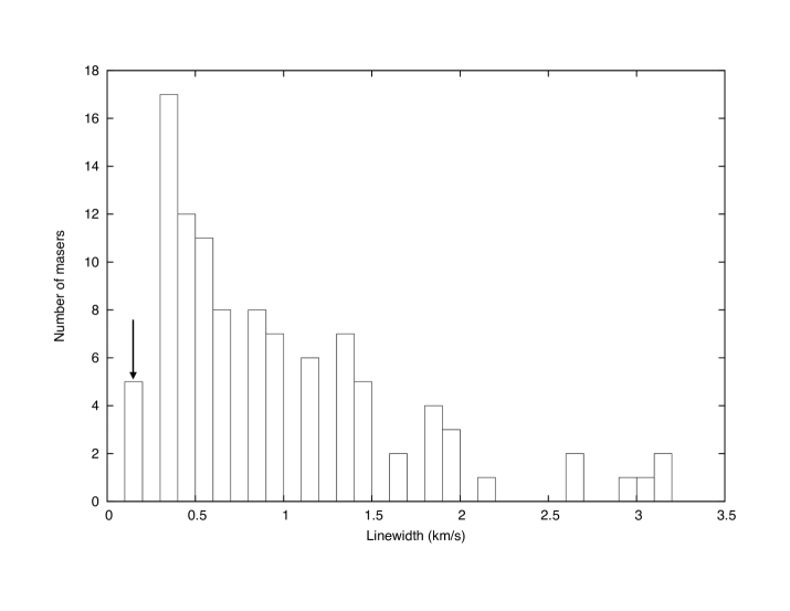
Figure 1: Distribution of maser linewidths (FWZI) for the whole sample. The arrow indicates the bin corresponding to our spectral resolution.

Figure 1 shows the linewidth distribution (FWZI as reported in Table 2) of the masers we detected. The peak of the distribution is at 0.3-0.4 km s^-1, and the median value is 1.0 km s^-1. The linewidths range from $\geq$ 0.17 km s^-1 (the channel width) to 3.15 km s^-1; we note that the wider linewidths may correspond to multiple un-resolved maser components and/or thermal contribution to the emission. Masers from both groups, HMPO and UC HII regions, have velocities covering nearly this full range; i.e., there is essentially no difference in the linewidths between the two groups.

An extensive interferometric survey of southern class I methanol masers (at both 36 and 44 GHz) was recently published by Voronkov et al. (2014). Their sample size (71 sources) was very similar to ours; their angular resolution ($6^{\prime\prime}$) was somewhat lower, but their spectral resolution (0.064 km s^-1) was nearly 3 times higher. Overall, the two surveys are sufficiently similar that it is worthwhile to compare results. The linewidth distribution that we show in Figure 1 is generally similar to that found by Voronkov et al. (2014). Both distributions rise sharply from the spectral resolution of the observations, peak at about 0.3 km s^-1, and fall-off steadily at greater linewidths. Our distribution is somewhat flatter (i.e., it falls off more slowly), which may occur because Voronkov et al. (2014) use the effective FWHM, based on multi-component Gaussian fits, while we use the FWZI. Voronkov et al. caution that all their narrow-line components arise from these multi-component fits, so that possibly the extreme narrowness of the distribution is a result of the fit systematics. The fact that our distribution peaks at a similar narrow value suggests that these fit systematics probably do not substantially affect the results.

Voronkov et al. (2014) report linewidths up to 8.0 km s^-1 and suggest that large linewidths ($>$ 1.5 km s^-1) seem to arise from weak wings of the maser emission, although they do not discard the possibility of quasi-thermal emission. Our broadest linewidth is 3.2 km s^-1. It is unclear if our narrower linewidths result from an intrinsic difference between the samples or if they are an observational artifact. The VLA data presented here have higher spatial resolution and (on average a factor of two) better sensitivity than the ATCA data presented by Voronkov et al. (2014). It is possible that we spatially resolve different spectral components that ATCA sees blended in position. Sensitive, high resolution (both angular and spectral) observations of the broader sources from the Voronkov et al. (2014) should be conducted.

5.1.2 Relative Velocity Distribution

The relative velocity distribution of the methanol masers is shown in Figure 2. We use the ammonia velocities reported by M96 for the systemic velocity of the cloud, and plot the difference of the maser velocities with respect to the cloud velocities. These relative velocities range from $-$2.7 to $+$3.8 km s^-1. The distribution peaks at $\sim$ 0.7 km s^-1, with a standard deviation of 1.2 km s^-1. The total range of velocities is less than 6.5 km s^-1. This is substantially less than the 18 km s^-1 range found for 6.7 GHz class II methanol masers by Szymczak & Kus (2000), but consistent with the 5 km s^-1 found by Fontani et al. (2010) for class I methanol masers (via single-dish observations). Voronkov et al. (2014) found that, apart from a small number of blue-shifted high-velocity masers (with offsets greater than 15 km s^-1), the distribution of relative maser velocities is centered around zero, with a mean value of $-0.57$ km s^-1, and standard deviation of $3.32$ km s^-1. Our distribution peaks at a marginally higher velocity and is noticeably narrower. A possible explanation for the latter difference is that we calculate the relative velocity with respect to ammonia, while Voronkov et al. (2014) use the middle of the 6.7 GHz methanol maser velocity range as the reference. We note that using ammonia as the reference, rather than 6.7 GHz methanol masers, results in relative velocities that differ by a few km s^-1. For example, comparing the 44 GHz maser velocities of IRAS 20126+4104 reported in this paper to the 6.7 GHz maser velocities reported by Surcis et al. (2014) results in a relative velocity 2.7 km s^-1 different from that found using ammonia as the reference. The wider distribution reported by Voronkov et al. (2014) may be caused by this effect. However, the absence of high-velocity features with offsets greater than 15 km s^-1 in our data is due the limited bandwidth of our observations ($\sim$ 20 km s^-1).

Some authors argue that the small relative velocity of these masers supports the idea that class I methanol masers arise in the interface region between outflows and cores (see Plambeck & Menten, 1990). We discuss the relation of masers with molecular outflows in $\S$ 5.2 and 5.6.

5.2 Comments on selected regions

Because the sample extends well into the second galactic quadrant, many of our sources do not have survey data (IR or radio) that are readily available. Ancillary observations at arc-second resolution exist for some sources of our sample, including observations of molecular tracers that allow us to make a comparison with protostellar outflows. The source of information is diverse: millimeter, near- and mid-IR observations. Here we discuss these data in the context of our 44 GHz methanol maser detections. With the exception of Mol 45 (for which recently published IR data are now available) sources that are common to Paper I are not re-discussed here, since no significant differences were found by the new observations. Given the attention during the last years of the correlation between Spitzer/IRAC images and class I methanol masers (e.g., Cyganowski et al. 2009), we discuss that correlation separately ($\S$ 5.6).

5.2.1 IRAS 05274+3345 (Mol 10)

Mol 10 does not present a high level of star formation activity; its IRAS luminosity is 3 $\times$ 10³ L_⊙, but molecular emission is very weak Estalella et al. (1993). About 30^′′ to the east of the IRAS source, centimeter and millimeter continuum emission reveal a cluster of five protostars (the AFGL 5142 region: Zhang et al. 2007; Hunter et al. 1999; Hunter et al. 1995). Associated with the continuum cores are at least three bipolar outflows. The main outflow (named outflow A by Zhang et al. 2007) was reported by Hunter et al. (1999) in a north-south direction in SiO emission, but recent mm/sub-mm observations show that at least two additional outflows are present in different directions (Zhang et al. 2007; see Fig. 3). Water masers and IR emission are coincident with shocked regions within the outflow lobes (Zhang et al. 2007; Hunter et al. 1995, 1999).

Our VLA observations do not show maser emission near the IRAS source, but masers are found to the east, near the molecular outflows (see Fig. 3; also $\S$ 5.6). The positions of the maser components in AFGL 5142 confirm their relation with the outflow lobes, as shown in Figure 3. All maser components seem to be associated with the western lobe of outflow C and possibly the southern, inner part of outflow B. Despite the positional coincidence with the outflows, the maser velocities are within a few km s^-1 of the systemic velocity ($-$3.8 km s^-1), while Zhang et al. (2007) report terminal velocities of 25 km s^-1 for outflows B and C. Thus, if the masers participate in the dynamics of the outflows, they should be related to its low-velocity component or the swept-up material.

5.2.2 IRAS 18144$-$1723 (Mol 45)

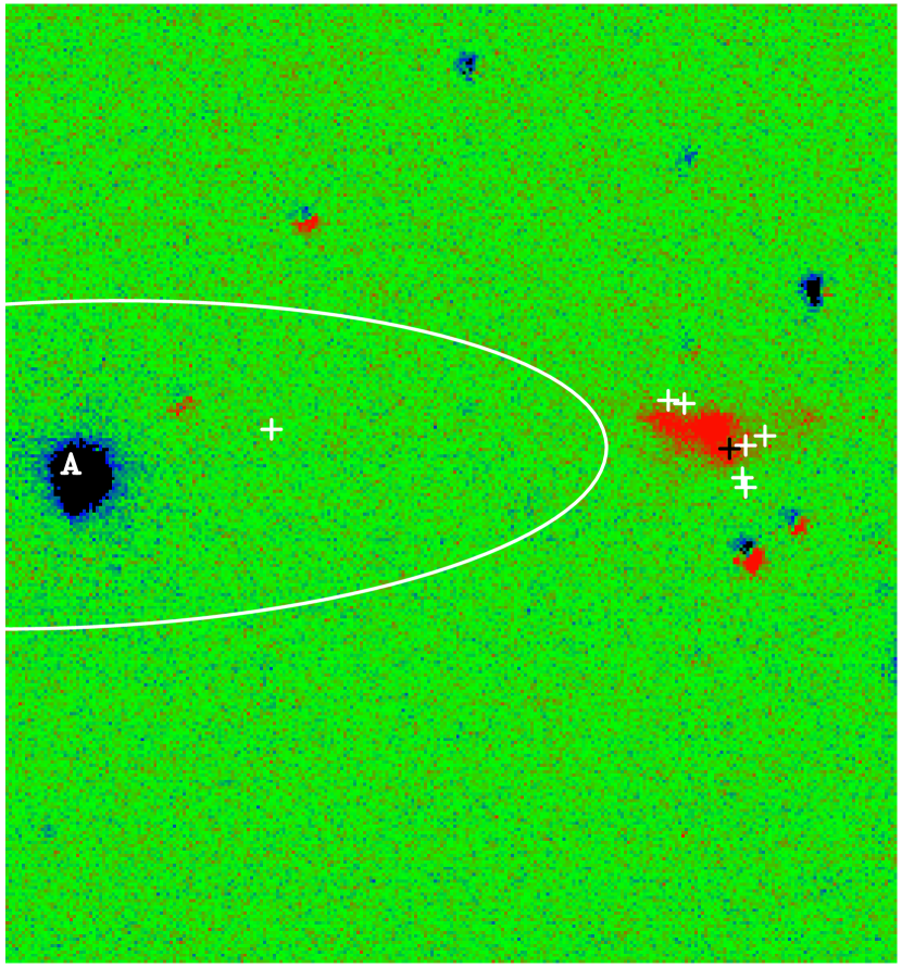
Figure 4: IRAS 18144$-$1723 (Mol 45). In false calors we show the continuum-subtracted H₂ image from Varricatt et al. (2010). Maser positions are shown by crosses. Nine of the maser spots we report are clustered near the bow-shock-like feature to the west of the image. The remaining two (overlapping) masers are further to the east, about 10^′′ from the infrared source ‘A’. The ellipse indicates the IRAS position.

Zhang et al. (2005) did not report an outflow in this field. Nevertheless, Varricatt et al. (2010) present an H₂ image showing a bowshock-like feature about 18^′′ to the west of the IRAS position (see Fig. 4). Coincident with the IRAS source, they detect a K-band continuum source which they call ‘A’, that has some surrounding nebulosity. They suggest that the bowshock-like feature originates from source A, and represents a highly collimated (factor 10) outflow at position angle 274^∘.

We detect 11 maser spots in this field. Nine of these (two of them overlap) fall in a cluster within about 5 arcsec of the bowshock feature reported by Varricatt et al. (2010). The two remaining (overlapping) masers are located about 10 arcsec west of the infrared source ‘A’ (Fig. 4).

5.2.3 IRAS 18507+0121 (Mol 74)

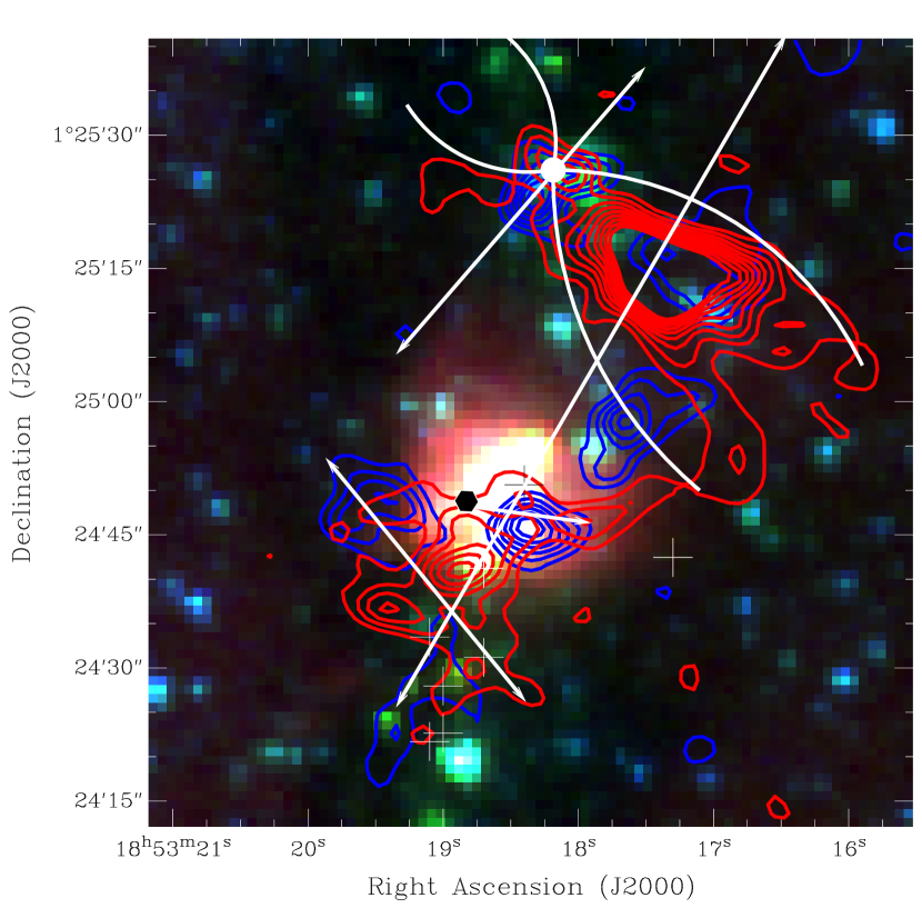
Figure 5: Overlay of high-velocity CO emission (red and blue contours) on the three color image from Spitzer (3.6, 4.5, 8.0 $\,\mu$m) toward IRAS 18507+0121 (Mol 74; Shepherd et al. 2007). The eight plus symbols show the 44 GHz methanol maser positions from this paper, while the white circle and black hexagon denote the millimeter source (MM1) and the UC HII region (MM2), respectively, reported by Shepherd et al. (2007). The white arcs and lines show the outflow systems proposed by Shepherd et al. (2007). Note that the maser spots are distributed closer to the UC HII region than to the millimeter source, and seem to be associated with 4.5$\,\mu$m emission excess.

This massive star forming region is located in an infrared dark cloud (IRDC) which hosts nine millimeter cores Shepherd et al. (2007). The millimeter core MM2 is associated with the IRAS source and an UC HII region Miralles et al. (1994); Molinari et al. (1998); see Fig. 5. The centimeter continuum flux is consistent with excitation by a ZAMS B0 star Shepherd et al. (2004). VLA observations show H₂O masers toward MM1, MM3 and MM4 Wang et al. (2006); only MM1 lies within the field shown in Fig. 5. These cores have bolometric luminosities of 3.2 $\times 10^{4}$, 9.0 $\times 10^{3}$, and 1.2 $\times 10^{4}$ L_⊙, respectively Rathborne et al. (2005), suggesting that they are high-mass protostars.

Shepherd et al. (2007) report three outflows centered on or near the UC H II region (G34.4+0.23; i.e., MM2), and two other outflows from the millimeter core G34.4+0.23 MM (MM1). Fig. 5 shows high-velocity CO emission tracing the molecular outflows overlaid with the 44 GHz maser positions. All the maser spots are located around the UC H II region, and some of them are coincident with the outflow lobes. No maser emission was found toward the outflows from MM1, although the VLA primary beam covered that region. This information suggests that, as in the case of Mol 10 (AFGL5142), class I methanol masers are located toward the more-evolved objects of the cluster (i.e. outflows from sources that already developed an UC H II region).

5.2.4 IRAS 18517+0437 (Mol 76)

Varricatt et al. (2010) report an embedded source located about 12^′′ south-west of the IRAS position. No collimated structure was found in H₂; rather, the H₂ line emission appears as a faint, arc-like feature $\sim 5^{\prime\prime}$ north-east of the embedded source. We detect three maser spots, distributed around the arc-like feature.

Interferometric observations by Schnee & Carpenter (2009) detected two masers in the 95 GHz class I transition. These masers (which they label $a$ and $b$) correspond (in position and velocity) to our masers 3 and 2, respectively.

5.2.5 IRAS 19374+2352 (Mol 109)

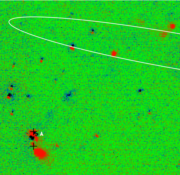
Figure 6: Same as Fig. 4 but for IRAS 19374$+$2352 (Mol 109). A few arcsec to the south of source ’A’, H₂ emission is seen, possibly tracing a collimated outflow. The 44 GHz masers are located within 5^′′ of source ’A’.

Varricatt et al. (2010) find H₂ emission associated with this source (which they label ‘A’) and note that it corresponds to a pair of stars separated by 1.^′′5 (see Fig. 6). A few arcsec to the south of source ’A’, H₂ emission is seen, possibly tracing a collimated outflow. Based on their data and previous mm-wave observations, Varricatt et al. (2010) infer the presence of multiple molecular outflows in the region, although they cannot identify the driving sources. If one of these stars is driving a molecular outflow, then the methanol masers would evidently arise near the base of the outflow, rather than at the interaction region of the outflow lobes with the interstellar medium. As seen in Fig. 6, the 44 GHz masers are located within 5^′′ of source ‘A’.

5.2.6 IRAS 20050+2720 (Mol 114)

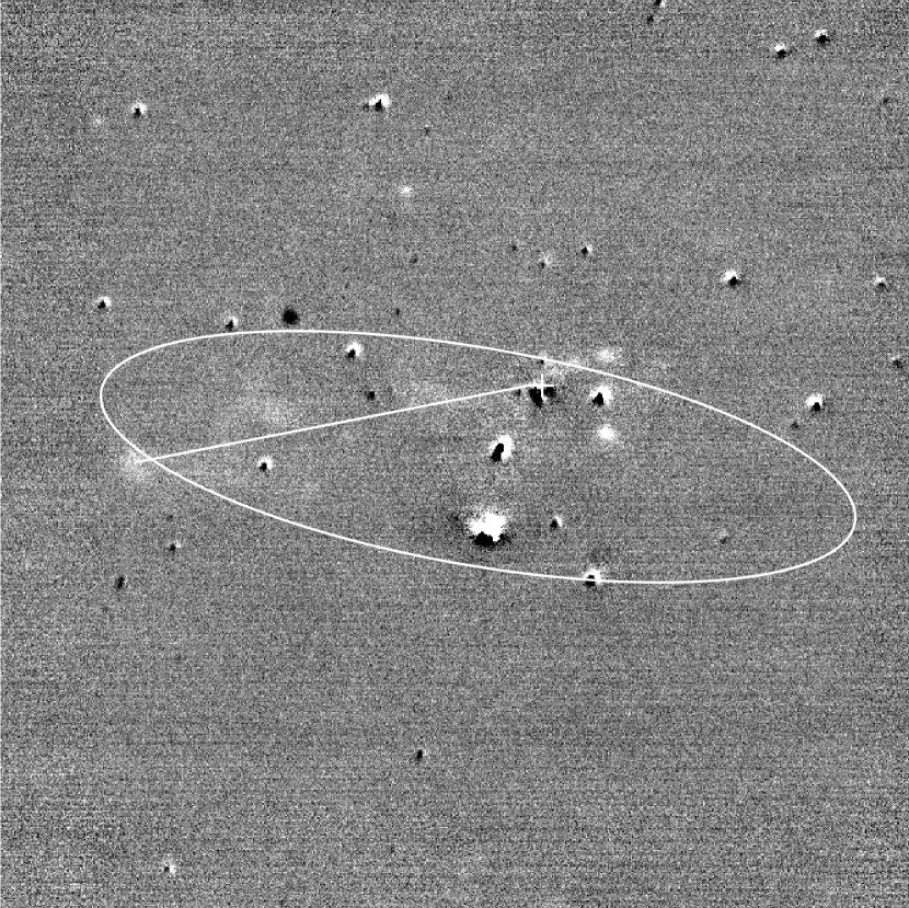
Figure 7: Same as Fig. 4 but for IRAS 20050$+$2720 (Mol 114). Varricat et al. (2010) suggested several outflows in the region. One lobe of the main outflow of the region is indicated by the white line, at the base of which, projected near to the proposed driving source ($<$ 2^′′), we see the 44 GHz methanol maser.

We detect a single maser component in this field, coincident with the millimeter continuum source OVRO 1 reported by Beltrán et al. (2008). Beltrán et al. conclude that two molecular outflows are present, and that their driving sources are OVRO 1 and a YSO within the 8000 AU (11.^′′3) envelope surrounding OVRO 1. The maser position that we report is less than 1^′′ from the OVRO 1 position, suggesting that the maser is associated with the east-west outflow, driven by OVRO 1, and that it arises near the base of the outflow. We caution that this interpretation is not unambiguous. Beltrán et al. suggest that the two outflows interact with one another; it is possible that the maser arises in an interaction region, rather than at the driving source of one of the outflows. Moreover, Varricatt et al. (2010) suggest that additional outflows might be present. If so, and if one of these were oriented along the line-of-sight, the maser could arise rather far from the outflow origin, but appear projected near ($<$ 2^′′) to the driving source (see Fig. 7).

5.2.7 IRAS 20056+3350 (Mol 115)

Although M98 did not detect radio continuum emission in this field, Jenness et al. (1995) report weak (0.6 – 0.9 mJy) 8 GHz emission located about 2^′′ from the maser positions. Although this continuum emission — located so close to the maser positions — is interesting, we do not count Mol 115 as a source with a UC HII region, because the quite low flux density suggests that the origin of the emission is not photoionization by a young, early-type star, but rather is due to some other mechanism (e.g., Rodríguez et al. 2012).

5.2.8 IRAS 20062+3550 (Mol 116)

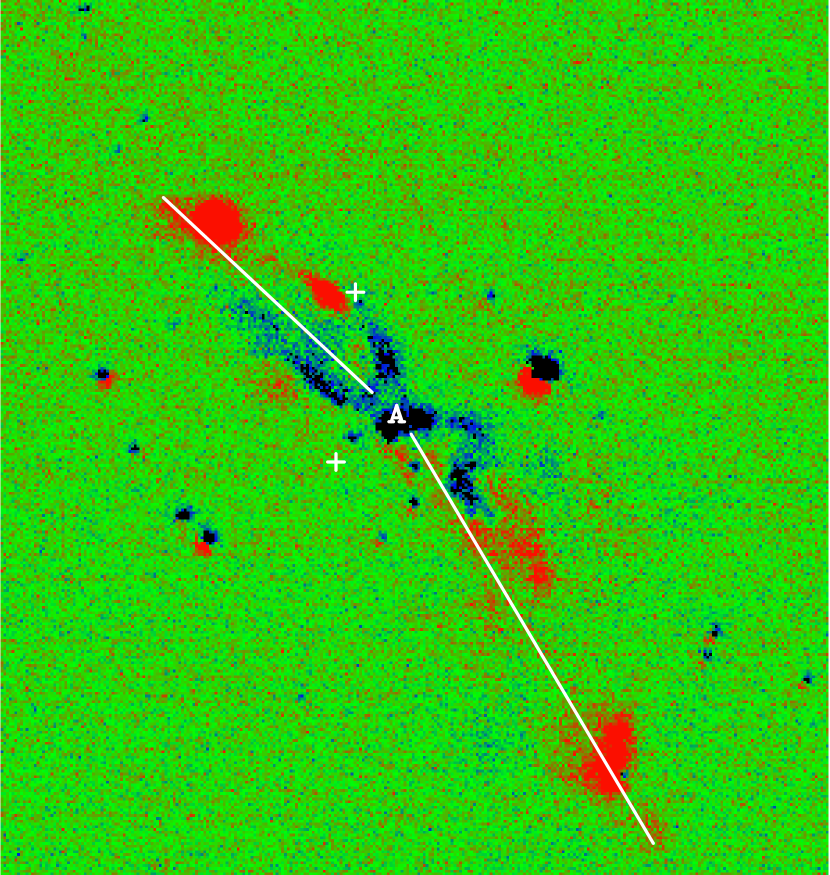
Figure 8: Same as Fig. 4 but for IRAS 20062$+$3550 (Mol 116). The proposed source ’A’ that drives a bipolar outflow, which has a lobe extending 10^′′ to the north-east and another extending 16^′′ to the south-west (indicated by white lines). Two 44 GHz detected relatively close (1.^′′4 and 4.^′′9) to the source ’A’.

Mol 116 hosts one of the larger molecular outflows reported by Zhang et al. (2005). The outflow has a far more spectacular appearance in the K-band and H₂ images of Varricatt et al. (2010), as seen in Fig. 8. They report an IR source ‘A’ as the probable driving source of the outflow, which has a lobe extending 10^′′ to the north-east and another extending $16^{\prime\prime}$ to the south-west. The two masers we detect are located relatively close (1.^′′4 and 4.^′′9) to source A. This is in contrast with the case of IRAS 20126$+$4104 (see Paper I) in which the masers coincide with the tips of the outflow lobes. In Mol 116 the masers seem to be located in the interaction zone between the inner part of the cavity wall and the surrounding medium. This behavior may also occur in Mol 114 and, possibly, Mol 109. Alternatively, the emission could arise from an undetected pole-on outflow produced by another central source.

5.2.9 IRAS 22506+5944 (Mol 151)

Single-dish and interferometric CO observations of the outflow in Mol 151 were reported by Wu et al. (2005) and Su et al. (2004), respectively. The single-dish map shows a north-south outflow, while the interferometer map (including single-dish data for the zero spacing) shows an east-west outflow. In both cases, the total angular extent of the molecular emission is of order 1 arcminute. The driving source of the outflow(s) has been attributed to both IRAS 22506+5944 and to the near-IR source S4 (2MASS J22523871+6000445; e.g., Xu & Wang, 2010).

The S4 position is nominally outside the IRAS error ellipse for 22506+5944. Nevertheless, we note that the 2MASS image shows a compact cluster of five sources that IRAS could not have resolved. We consider the IRAS source to correspond to the cluster, not to its individual members, and disregard the precise IRAS coordinates.

More importantly, we note that all six maser components that we detect are within 9^′′ of the S4 position (see Figure 7 of Su et al. 2004) while the two outflow lobes span 1^′ in the east-west direction. Thus, as in several previous cases, the masers might trace the base of the outflow and not the terminus of the outflow lobes.

5.3 44 GHz methanol masers in HMPO’s and UC HII regions

Molinari et al. (1998) observed 67 sources from their larger sample in the 6 cm continuum with the VLA, and detected emission at the 1 mJy level (or higher) in 37 (55%) of the sources. If the centimeter continuum emission was within 40^′′ of the IRAS position, then they considered the continuum emission to be an IRAS-related UC H II region; 22 sources were in this category. In Table 1 we list sources as “UC H II regions” if the free-free emission is within 40^′′ of the corresponding IRAS source. As we note in §2, in some cases this centimeter continuum may arise from some other class of object than a UC H II region (e.g., a thermal jet). On the other hand, if there is no detected centimeter free-free emission ($\gtrsim$ 1 mJy), or if it is more than 40^′′ distant, we define the source as a “HMPO”.

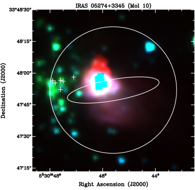
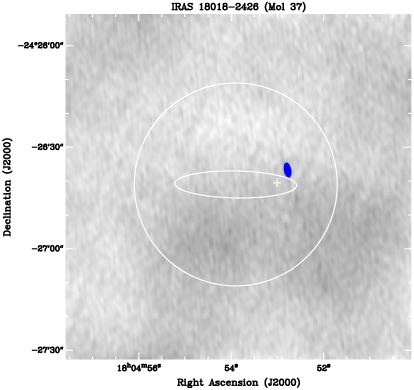
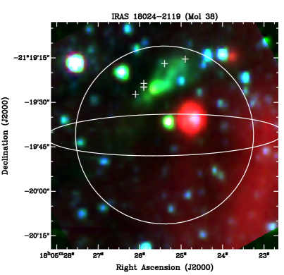
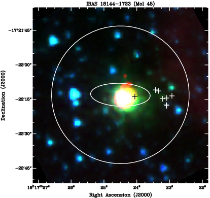
Figure 12: Three-color images from IRAC/Spitzer (3.6$\mu$m: blue, 4.5$\mu$m: green, 8.0$\mu$m: red). 44 GHz methanol masers are represented by plus symbols, the IRAS position is indicated by the ellipse, while the VLA primary beam by a circle. When available, the 3.6 cm continuum from Molinari et al. (1998) is shown in blue contours (in steps of 10% of the peak). When only the 3.6 cm continuum is available, the emission is shown in grey scale and blue contours.

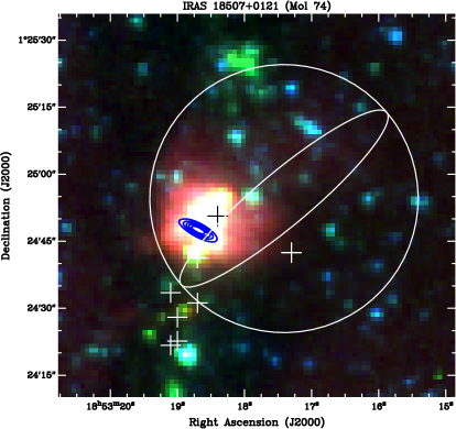
Figure 12: Cont.

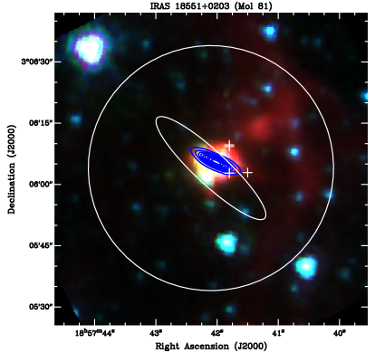
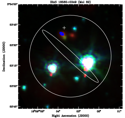
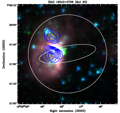
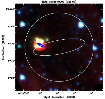
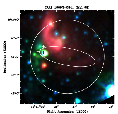
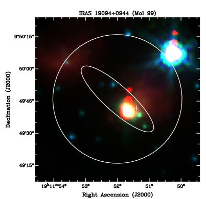
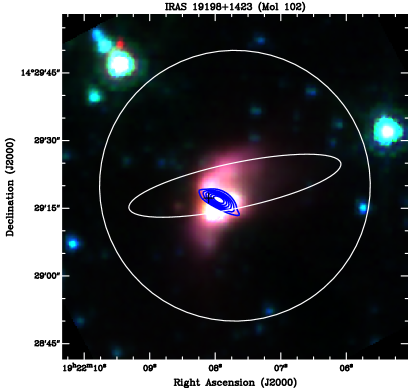
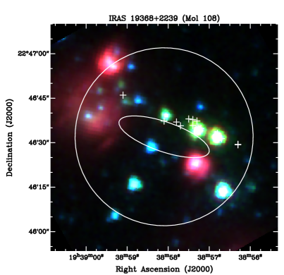
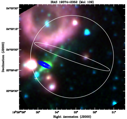
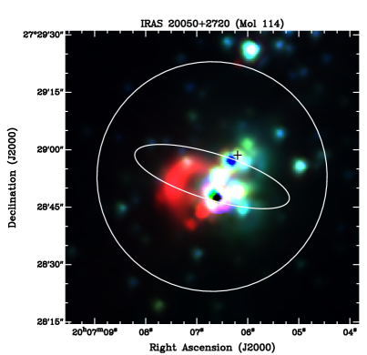
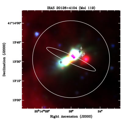
Figure 12: Cont.

We show the location of the masers with respect to the continuum emission (from M98) in Fig. 12, where the centimeter continuum emission from Molinari et al. (1998) is shown by contours. For the 13 UC HII sources showing maser emission, we measure the projected distance from each maser component to the peak position of the continuum emission (based on the source distances in Table 1 and the continuum positions reported by M98). The resulting projected distances are shown in Fig. 9. The shortest separation measured is 0.005 pc and the largest is 0.6 pc. In four sources some maser components are projected against the centimeter emission. This result is consistent with that of Kurtz at al. (2004) that class I methanol masers can be found in the immediate vicinity of UC HII regions.

Excluding the three sources that we were unable to calibrate, we find that 13 of 24 ($54$ %) of the UC H II fields show maser emission, while 16 of 42 HMPO fields (38 %) show masers. The sample sizes are not large enough for this result to have a firm statistical basis, nevertheless, these detection rates suggest that class I methanol masers are more common in the presumably more-evolved regions of the Molinari sample that present centimeter free-free emission. Voronkov et al. (2014) find a much lower association of class I maser emission with centimeter continuum emission (17 of 71 sources or 24%). However, as they note, their continuum data are very inhomogeneous, so this association rate should be treated as a lower limit. We caution that assigning evolutionary stages based on the presence or absence of particular maser species may not be always reliable. We refer the interested reader to §4.5 of Voronkov et al. (2014), which presents an enlightening discussion of this point.

5.4 Color-color analysis

Color-color diagrams applied to different maser species have proven useful to search for trends in maser and far-IR properties (e.g., H₂O: Palla et al., 1991; class II CH₃OH: Szymczak & Kus, 2000; OH: Edris et al. 2007). In Figure 10 we present the color-color diagram [25-12] versus [60-12]; the limits for High and Low sources follow the M96 classification. Excluding the three sources we were unable to calibrate, our sample contains 30 High and 36 Low sources. The maser detection rates are 19 out of 30 for High ($\sim$ 63 %) and 10 out of 36 for Low ($\sim$ 27 %). As pointed out previously, the High classification corresponds to sources with colors meeting the Wood & Churchwell (1989) criteria for UC H II regions. Inspection of the color-color plot shows that in general the detection rate increases toward the redder corner (upper right) of the box. In particular, a maser detection rate of $70\%$ is found in the region [25-12] $>$ 0.90 and [60-12] $>$ 1.99. This is in agreement with Fontani et al. (2010), who found a 3 times higher detection rate in the High region compared to the Low region.

Palla et al. (1991), using a much larger sample, found that water masers are common in sources with the Wood & Churchwell (1989) colors. Their water maser detections were bounded by [25-12] $\geq$ 0.1 and [60-12] $\geq$ 1.1. They found that setting the [25-12] index to $\geq$ 0.50 did not affect the detection rate, and concluded that a [25-12] index larger than 0.5 is a reliable indicator for far-IR sources associated with H₂O maser emission. They found a $50\%$ detection rate for H₂O masers when [60-12] $>1.8$ and [25-12] $>0.9$. For OH masers, Edris et al. (2007) combined the M96 and Sridharan et al. (2002) samples, and report masers for color indices [25-12] $\geq$ 0.23 and [60-12] $\geq$ 1.1 (i.e., higher detection rates toward redder sources). Also, sources with OH masers dominate over non-maser sources for regions with [25-12] $>$ 1.2 and [60-12] $>$ 2.2. In the case of class II CH₃OH masers, Szymczak & Kus (2000) found that the highest detection rates were for intermediate colors. Their maximum detection rate was found near 0.8 $<$ [25-12] $<$ 1.0 for [60-25] $<$ 0.8.

Our results show that class I CH₃OH masers follow similar trends to OH, H₂O and class II CH₃OH masers with respect to the far-IR colors of the host region. We caution that any color-color trend between High and Low sources must be tested independently from a luminosity effect. M96 report a one-quarter dex higher luminosity for the High sources compared to the Low sources (see their Table 4 and Figure 6). Thus, differences between the two groups may arise from differing luminosities, rather than differing colors.

5.5 Maser luminosity and IRAS properties

To discern the relation of maser emission with other star formation processes, we looked for correlations between the isotropic maser luminosity and the parameters of the central source. The maser flux density of each field and the source distance (taken from M96) were used to calculate the isotropic maser luminosity. In the case of multiple maser components, we summed the individual flux densities and used this value to obtain the luminosity.

Figure 11 shows a plot of isotropic maser luminosity versus IRAS luminosity. For IRAS luminosities greater than $10^{3}$ L_⊙ there is no obvious correlation between the maser and infrared luminosities. The four sources with IRAS luminosities below $10^{3}$ L_⊙ have maser luminosities about two orders of magnitude lower than the rest of the sample, suggesting that there is a tendency toward higher maser luminosity as the IRAS luminosity increases. However, it is possible that the kinematic distances reported by M96 are inaccurate. In particular, we note that the distances of these four low-luminosity sources are uncertain and range from 80 to 730 pc, thus, their luminosity could have been understimated. If these distances are correct, then the sources Mol 38, Mol 114, Mol 116, and Mol 121 are low-to-intermediate mass star-forming regions, not high-mass star-forming regions. If so, we detected methanol masers from non-high-mass star-forming regions — unusual for methanol masers (Kalenskii et al. 2013).

In summary, we consider the distances, luminosities, and classifications of these four sources to be uncertain. A definitive determination of their distances is needed before we can ascertain the significance of the trend of lower maser luminosity with lower IRAS luminosity, and to investigate whether new “low-mass” methanol masers have been found.

5.6 Relation with mid-IR emission from Spitzer/IRAC

A relation between class I methanol masers and molecular outflows was proposed by Plambeck & Menten (1990) based on interferometric observations of the 95 GHz transition in DR21. They found that the maser positions coincided with H₂ emission from shocked gas along the outflow lobes. Subsequent interferometric observations have supported the outflow-maser association Johnston et al. (1992); Kurtz et al. (2004); Voronkov et al. (2006); Araya et al. (2009). Several of the sources discussed in section 5.2 exemplify this relation. To study the maser–outflow connection in our sample, we use publicly available Spitzer images.

An important indicator of shocked regions in outflows is the mid-IR emission from ro-vibrational H₂ transitions and/or CO bandheads covered by the Infrared Array Camera (IRAC; Fazio et al. 2004). The $\lesssim$ 2^′′ angular resolution of IRAC is similar to that of many millimeter interferometric observations of CO and SiO lines, allowing for useful comparisons. The 4.5$\,\mu$m band includes emission from HI Br$\alpha$, CO(J=1-0) P(8) fundamental bandhead, several H₂ lines, and some forbidden molecular lines; notably, no PAH emission is found in this band. Thus, the 4.5$,\mu$m band mostly traces shocked and/or ionized gas (Shepherd et al. 2007). Very bright H₂ emission and/or broad CO bandhead emission can produce an excess in the 4.5$\,\mu$m band, with respect to the 3.6$\,\mu$m and 8.0$\,\mu$m bands (e.g., Shepherd et al. 2007, Smith et al. 2006). A 4.5$\,\mu$m excess therefore indicates the presence of shocked molecular gas. We searched the Spitzer archive for IRAC observations toward our sample of massive protostars. Not all the fields were observed by Spitzer. Most of the images retrieved were observed as part of the GLIMPSE survey (Benjamin et al. 2003).

In Fig. 12 we show the three-color images of the 3.6, 4.5, and 8.0$\,\mu$m bands, with overlays of the 44 GHz maser spots. A spatial coincidence of the masers and the mid-IR emission is seen in most of the sources. In at least half of the sources we find a 4.5$\,\mu$m excess, indicating the presence of shocked gas, possibly related with outflows. In most cases, the methanol masers lie close to or coincident with the 4.5$\,\mu$m excess.

A similar comparison between 44 GHz class I methanol masers and 4.5$\,\mu$m excess emission is given by Cyganowski et al. (2009). They observed 44 GHz class I masers with the VLA toward a GLIMPSE-selected sample of sources with extended 4.5$\,\mu$m excess (the so-called Extended Green Objects or EGOs). Their observations show several cases in which class I methanol masers surround the EGOs. This pattern is also found in some of our observations; see, for example, IRAS 18024$-$2119 (Mol 38) and IRAS 20126+4104 (Mol 119) shown in Figure 12. This behavior suggests that class I methanol masers are tracing the interface between the outflow lobes and the surrounding material, as originally proposed by Plambeck & Menten (1990). In addition, the small relative velocities reported in §4.2.2 may relate these masers with the post-shock gas (entrained material) in outflows.

This spatial coincidence in a substantial fraction of our sample is strong circumstantial evidence to support the idea of a physical origin of the masers in shocked, possibly outflowing gas. Nevertheless, we note that about half of the Spitzer images show no evidence for a 4.5$\,\mu$m excess, despite the fact that 44 GHz masers are detected. Although the maser emission usually is closely associated with mid-IR emission, there are at least two cases (IRAS 18144$-$1723 and IRAS 18565+0349) in which the masers appear to be isolated, with no nearby mid-IR emission. A plausible explanation for these two cases is that the masers trace shocks from a very deeply embedded object, similar to the case of DR21(OH) in which the outflow and driving source are not detected in the mid-IR (Araya et al. 2009).

Particularly intriguing is our finding that in four cases, the masers may be located close to the putative base of a molecular outflow. As we mention in §4.3, the projected maser positions of various sources fall close to the presumed driving source of the outflow. In particular, the Molinari sources 109, 114, 116, and 151 show this behavior. Of course, lying close to the base of the outflow does not preclude the possibility that the masers arise in shocked gas, and perhaps this is produced by an orientation affect [e.g., a pole-on (undetected) outflow]. The interpretation of this result is not yet clear; but it is in contrast to the finding of other studies (e.g., Kurtz et al. 2004, Araya et al. 2009, Cyganowski et al. 2009) in which the masers are found at the outer end of the outflow lobes, rather distant from the driving source.

In §5.2 (see also Figures 3 and 5) we showed two cases in which class I masers in regions with multiple outflows appeared toward the more-evolved sources. In these two cases the outflows where the masers were found are also related to HII regions, suggesting that class I masers may trace an evolved phase of the outflow. Other authors have reported the relation of class I methanol masers and HII regions, suggesting that expanding HII regions might be another shock environment in which class I masers are excited (e.g., Voronkov et al. 2010, Sobolev 1992).

In a larger context, this and other surveys of class I methanol masers not only suggest that these masers may trace shocks at different stages, but may even trace shocks arising from a number of different phenomena occurring in star-forming regions. Class I masers in regions with little or no mid-IR emission may trace deeply embedded shocks from ’young’ bipolar outflows or cloud-cloud collisions (this work, Araya et al. 2009, Plambeck & Menten, 1990). In IR-bright regions with a 4.5 micron excess, and therefore with strong shocks, the class I masers are found tracing bow-shocks of ’young’ outflows (e.g., this work, Cyganowski et al. 2009). For regions with cm-continuum emission, the class I masers may trace bow-shocks from ’old’ outflows and/or expanding HII regions (e.g., this work, Voronkov et al. 2010, Voronkov et al. 2014).

6 Summary and Conclusions

The principal results of this survey of 44 GHz class I methanol masers are the following:

A 38% (16/42) maser detection rate was found toward HMPO candidates, while 54% (13/24) was the detection rate in fields with candidate UC HII regions. These detection rates suggest that although class I methanol masers are found in both HMPO and UC HII regions, they are more common in more-evolved regions.

Toward UC HII regions, the projected distance from the maser spots to the peak of the continuum emission was between 0.01 and 0.6 pc. In some cases the masers are projected onto the ionized regions.

In comparison with other similar interterferometric data sets, our observations show narrower linewidths, likely due to our higher spatial resolution. Also, the relative velocity distribution is noticeably narrower, but in this case possibly due to the different method used to determine the cloud velocity. High-velocity class I methanol masers reported by other authors may have been missed by our observations, because our limited bandwidth.

In two fields, possessing both young and old outflows, the masers were only found toward the more-evolved outflows. This is suggestive that class I methanol masers also trace later stages of outflow evolution. However, other authors have reported these masers towards tracers of ’young’ outflows. Therefore, assigning evolutionary stages based on the presence or absence of particular maser species may not be always reliable.

Based on a comparison with observations of molecular outflows in the millimeter and IR, we find evidence that the masers are sometimes located at the interface between the molecular outflow and the surrounding material. In addition, the small relative velocities ($\leq$4 km s^-1) between the masers and the ambient molecular material suggests that the former are located in post-shock regions (entrained material) of molecular outflows. The presence of a number of class I masers that are not obviously associated with shocked gas, and which in some cases appear to arise very close to the base of the outflow, suggests that more than one scenario may be needed to understand the occurrence of 44 GHz class I methanol masers.

This and other surveys of class I methanol masers not only suggest that these masers may trace shocks at different stages, but may even trace shocks arising from a number of different phenomena occurring in star-forming regions: young/old outflows, cloud-cloud collisions, expanding H II regions, among others.

Table 1: Observed Source List

Mol	IRAS	$\alpha$(J2000)	$\delta$(J2000)	Central Vel	Dist.	Synth Beam	Channel rms	44 GHz	UC HII
Num	Num	h m s	°0′0″	km s-1	kpc	arcsec	mJy beam-1	masers	Outflow
2 H	00117+6412	00 14 27.7	+64 28 46	$-$36.3	1.8	2.37$\times$1.75	56	0	UO
3 L	00420+5530	00 44 57.6	+55 47 18	$-$51.2	7.7	1.78$\times$1.70	46	0	O
7 H	04579+4703	05 01 39.7	+47 07 23	$-$16.5	2.4	1.79$\times$1.63	53	0
8 L	05137+3919	05 17 13.3	+39 22 14	$-$25.4	10.8	1.87$\times$1.51	48	0	O
9 H	05168+3634	05 20 16.2	+36 37 21	$-$15.1	6.0	1.89$\times$1.51	54	0	O
10 H	05274+3345	05 30 45.6	+33 47 52	$-$3.8	1.5	1.82$\times$1.52	52	8	O
11 L	05345+3157	05 37 47.8	+31 59 24	$-$18.4	1.8	1.80$\times$1.48	58	0	O
12 L	05373+2349	05 40 24.4	+23 50 54	+2.3	1.1	1.83$\times$1.48	52	0	O
15 H	06056+2131	06 08 41.0	+21 31 01	+2.6	1.5	1.88$\times$1.50	60	0	UO
28 L	06584$-$0852	07 00 51.5	$-$08 56 29	+41.3	4.4	2.72$\times$1.53	62	0	O
30 L	17450$-$2742	17 48 09.3	$-$27 43 21	$-$16.6	0.1	3.04$\times$1.33	82	0
36 L	18014$-$2428	18 04 29.6	$-$24 28 47	+13.0	2.8	2.65$\times$1.36	75	0
37 L	18018$-$2426	18 04 53.9	$-$24 26 41	+10.7	1.5	2.61$\times$1.37	96	1	UO
38 L	18024$-$2119	18 05 25.4	$-$21 19 41	+0.5	0.1	2.33$\times$1.41	58	6
39 L	18024$-$2231	18 05 30.6	$-$22 31 36	+16.1	2.9	2.47$\times$1.38	67	0
45 L	18144$-$1723	18 17 24.5	$-$17 22 13	+47.3	4.3	2.31$\times$1.55	54	11
50 L	18162$-$1612	18 19 07.5	$-$16 11 21	+61.7	4.8	2.28$\times$1.54	53	2	U
57 L	18256$-$0742	18 28 20.5	$-$07 40 22	+36.7	2.9	2.03$\times$1.57	48	0
59 L	18278$-$1009	18 30 35.2	$-$10 07 12	+97.7	5.7	2.02$\times$1.60	44	0
60 L	18288$-$0158	18 31 26.7	$-$01 56 35	+3.8	0.5	1.76$\times$1.64	41	0
66 L	18363$-$0554	18 39 03.7	$-$05 52 15	+65.2	4.3	1.88$\times$1.67	44	0
68 L	18396$-$0431	18 42 18.8	$-$04 28 37	+97.4	6.0	1.84$\times$1.66	48	2	UO
70 L	18424$-$0329	18 45 03.3	$-$03 26 49	+47.9	3.3	1.89$\times$1.69	44	0
74 H	18507+0121	18 53 17.4	+01 24 55	+57.2	3.8	1.83$\times$1.74	45	10	U
75 L	18511+0146	18 53 38.1	+01 50 27	+56.5	3.8	1.99$\times$1.40	39	1	O
76 H	18517+0437	18 54 13.8	+04 41 32	+43.7	3.0	1.88$\times$1.42	35	3
77 L	18527+0301	18 55 16.5	+03 05 07	+75.8	5.2	1.97$\times$1.36	46	1
78 H	18532+0047	18 55 50.7	+00 51 22	+58.4	3.9	1.91$\times$1.45	36	3	UO
81 H	18551+0302	18 57 42.1	+03 06 04	+57.0	3.9	1.89$\times$1.46	41	5	U
82 L	18565+0349	18 59 03.4	+03 53 22	+91.5	6.7	2.07$\times$1.46	37	1	U
84 L	18567+0700	18 59 13.6	+07 04 47	+29.4	2.1	1.77$\times$1.46	42	0	U
86 L	18571+0349	18 59 40.0	+03 53 35	+56.2	3.8	1.78$\times$1.47	38	0
87 L	18586+0106	19 01 10.6	+01 11 16	+38.0	2.7	1.89$\times$1.53	44	0
91 L	19012+0505	19 03 43.5	+05 09 49	+40.4	2.8	1.79$\times$1.42	46	0	U
93 H	19043+0726	19 06 47.7	+07 31 38	+58.9	4.3	1.71$\times$1.43	61	1	U
97 H	19088+0902	19 11 15.9	+09 07 27	+59.6	4.7	1.68$\times$1.39	59	1	U
98 L	19092+0841	19 11 37.4	+08 46 30	+58.0	4.4	1.62$\times$1.44	58	5
99 H	19094+0944	19 11 52.0	+09 49 46	+65.3	6.1	1.85$\times$1.45	65	1
102 H	19198+1423	19 22 07.7	+14 29 20	+58.9	5.5	1.66$\times$1.38	36	1	U
103 H	19213+1723	19 23 37.0	+17 28 59	+41.7	4.1	1.71$\times$1.45	44	0	UO
104 H	19282+1814	19 30 28.0	+18 20 53	+24.1	2.1	1.95$\times$1.53	171	0	O
108 H	19368+2239	19 38 58.1	+22 46 32	+36.4	4.4	1.92$\times$1.55	80	12	O
109 H	19374+2352	19 39 33.2	+23 59 55	+36.9	4.3	1.91$\times$1.44	84	2	UO
110 H	19388+2357	19 40 59.4	+24 04 39	+34.6	4.2	1.81$\times$1.39	113	2	UO
114 H	20050+2720	20 07 06.7	+27 28 53	+6.4	0.7	1.79$\times$1.49	89	1	O
115 H	20056+3350	20 07 31.5	+33 59 39	+9.4	1.6	1.76$\times$1.45	83	2	O
116 H	20062+3550	20 08 09.8	+35 59 20	+0.6	0.0	1.81$\times$1.39	113	2	O
117 L	20099+3640	20 11 46.4	+36 49 37	$-$36.4	8.6	1.75$\times$1.55	49	0	UO
118 L	20106+3545	20 12 31.3	+35 54 46	+7.8	1.6	1.92$\times$1.64	51	0	O
119 H	20126+4104	20 14 26.0	+41 13 32	$-$3.9	4.1	1.80$\times$1.57	43	5	O
121 H	20188+3928	20 20 39.3	+39 37 52	+1.5	0.3	1.68$\times$1.45	40	1	UO
122 L	20217+3947	20 23 31.7	+39 57 23	$-$0.9	3.7	1.69$\times$1.45	43	0
123 H	20220+3728	20 23 55.7	+37 38 10	$-$2.7	4.4	1.74$\times$1.52	46	0	UO
125 L	20278+3521	20 29 46.9	+35 31 39	$-$4.5	5.0	1.66$\times$1.40	42	0	O
126 H	20286+4105	20 30 27.9	+41 15 48	$-$3.8	3.7	1.83$\times$1.39	111	2	O
129 L	20333+4102	20 35 09.5	+41 13 18	+8.4	0.1	1.92$\times$1.46	217	0	U
131 H	20444+4629	20 46 08.3	+46 40 41	$-$4.1	2.4	1.90$\times$1.39	165	0	U
133 H	21078+5211	21 09 25.2	+52 23 44	$-$6.1	1.4	1.88$\times$1.43	151	0	UO
136 L	21307+5049	21 32 31.5	+51 02 22	$-$46.7	4.9	-	-		UO
138 H	21391+5802	21 40 42.4	+58 16 10	+0.4	0.7	-	-		O
139 H	21519+5613	21 53 39.2	+56 27 46	$-$63.2	7.3	-	-		O
143 L	22172+5549	22 19 09.0	+56 04 45	$-$43.8	2.8	1.77$\times$1.46	43	0	O
145 H	22198+6336	22 21 27.6	+63 51 42	$-$11.3	1.2	1.81$\times$1.43	49	0	O
148 H	22305+5803	22 32 24.3	+58 18 58	$-$51.9	5.4	1.65$\times$1.46	37	0	O
151 H	22506+5944	22 52 38.6	+60 00 56	$-$51.4	5.7	1.65$\times$1.46	39	6	O
154 L	23026+5948	23 04 45.7	+60 04 35	$-$51.1	5.7	2.19$\times$1.42	84	0
155 L	23140+6121	23 16 11.7	+61 37 45	$-$51.5	6.4	2.19$\times$1.67	60	0	UO
158 L	23314+6033	23 33 44.4	+60 50 30	$-$45.4	2.7	2.30$\times$1.37	61	0	O
160 L	23385+6053	23 40 53.2	+61 10 21	$-$50.0	6.9	2.14$\times$1.43	59	3	O

Table 2: 44 GHz Masers

		Maser Peak Position
Source	Maser	$\alpha$(J2000)	$\delta$(J2000)	$v_{LSR}$	$S_{\nu}$	FWZI	$\int S_{\nu}dv$
IRAS (Mol)	Number	h m s	°0′0″	km s-1	Jy	km s-1	Jy km s-1	Note
05274+3345 (10)	1	05 30 47.17	$+$33 47 58.1	$-$3.0	0.61	0.83	0.28
	2	05 30 47.53	$+$33 47 56.1	$-$2.8	2.00	1.83	1.18
	3	05 30 47.62	$+$33 47 52.2	$-$3.5	2.93	1.16	0.84
	4	05 30 47.62	$+$33 47 52.2	$-$4.3	0.44	-	-
	5	05 30 47.68	$+$33 47 56.5	$-$3.1	0.53	1.49	0.27
	6	05 30 47.68	$+$33 47 56.5	$-$3.7	0.15	-	-
	7	05 30 47.80	$+$33 47 55.3	$-$2.8	0.49	0.66	0.15
	8	05 30 47.98	$+$33 47 56.3	$-$3.0	0.40	0.83	0.22
18018-2426 (37)	1	18 04 53.01	$-$24 26 40.5	$+$10.9	579.41	1.16	329.51
18024-2119 (38)	1	18 05 24.94	$-$21 19 15.4	$-$1.0	0.69	1.00	0.42
	2	18 05 25.39	$-$21 19 16.9	0.0	11.19	1.49	6.44
	3	18 05 25.86	$-$21 19 24.8	$-$0.3	2.67	1.83	0.57
	4	18 05 25.86	$-$21 19 24.8	$+$1.8	0.36	0.17	0.01
	5	18 05 25.89	$-$21 19 23.6	$-$0.8	2.79	0.66	1.01
	6	18 05 26.10	$-$21 19 27.2	$+$2.5	0.56	0.50	0.19
18144-1723 (45)	1	18 17 22.93	$-$17 22 13.5	$+$48.3	6.82	2.99	5.55
	2	18 17 23.09	$-$17 22 14.4	$+$49.0	5.27	1.33	1.05
	3	18 17 23.09	$-$17 22 14.4	$+$49.7	0.14	-	-
	4	18 17 23.09	$-$17 22 17.8	$+$48.6	0.28	1.99	0.33
	5	18 17 23.10	$-$17 22 17.4	$+$47.5	0.59	-	-
	6	18 17 23.22	$-$17 22 14.7	$+$47.6	1.05	3.15	1.48
	7	18 17 23.43	$-$17 22 10.9	$+$46.6	0.39	-	-
	8	18 17 23.34	$-$17 22 11.3	$+$47.3	9.37	1.99	3.64
	9	18 17 23.34	$-$17 22 11.3	$+$46.0	1.28	-	-
	10	18 17 24.07	$-$17 22 13.8	$+$48.5	45.14	2.66	16.31
	11	18 17 24.06	$-$17 22 13.8	$+$48.0	14.34	-	-
18162-1612 (50)	1	18 19 07.60	$-$16 11 24.6	$+$64.0	1.09	0.66	0.46
	2	18 19 07.63	$-$16 11 25.4	$+$62.2	11.19	1.16	6.82
18396-0431 (68)	1	18 42 17.91	$-$04 28 56.5	$+$97.4	0.34	0.83	0.52
	2	18 42 17.88	$-$04 28 55.6	$+$97.1	0.34	-	-
18507+0121 (74)	1	18 53 17.30	$+$01 24 42.4	$+$54.9	1.40	1.66	0.98
	2	18 53 17.30	$+$01 24 42.4	$+$55.5	0.82	-	-
	3	18 53 18.46	$+$01 24 50.6	$+$58.2	1.33	1.16	0.51
	4	18 53 18.68	$+$01 24 41.2	$+$60.2	21.12	2.66	7.76
	5	18 53 18.69	$+$01 24 41.2	$+$59.7	6.85	-	-
	6	18 53 18.73	$+$01 24 31.1	$+$58.9	5.69	3.15	4.55
	7	18 53 19.07	$+$01 24 22.6	$+$57.5	0.69	0.33	0.15
	8	18 53 19.05	$+$01 24 27.9	$+$57.7	2.65	0.50	0.75
	9	18 53 19.06	$+$01 24 33.4	$+$59.7	3.42	1.33	2.05
	10	18 53 19.13	$+$01 24 21.7	$+$58.7	0.42	0.33	0.08
18511+0146 (75)	1	18 53 37.71	$+$01 50 25.5	$+$56.3	1.14	0.50	0.39
18517+0437 (76)	1	18 54 13.81	$+$04 41 34.0	$+$42.2	0.33	0.33	0.09
	2	18 54 14.46	$+$04 41 44.5	$+$44.2	1.28	1.83	1.05
	3	18 54 14.73	$+$04 41 42.9	$+$43.5	3.32	1.00	2.30
18527+0301 (77)	1	18 55 16.77	$+$03 05 06.9	$+$75.5	1.00	0.33	0.27
18532+0047 (78)	1	18 55 51.18	$+$00 51 12.3	$+$56.9	0.66	0.33	0.20
	2	18 55 51.34	$+$00 51 26.4	$+$60.6	0.81	1.33	0.66
	3	18 55 51.35	$+$00 51 26.4	$+$62.2	0.37	0.83	0.24
18551+0302 (81)	1	18 57 41.57	$+$03 06 02.9	$+$56.0	0.71	0.50	0.24
	2	18 57 41.81	$+$03 06 02.7	$+$56.0	2.88	0.83	1.17
	3	18 57 41.81	$+$03 06 02.7	$+$54.7	0.91	1.00	0.58
	4	18 57 41.87	$+$03 06 09.2	$+$56.3	0.54	0.50	0.19
	5	18 57 41.87	$+$03 06 09.6	$+$55.3	0.41	0.50	0.16
18565+0349 (82)	1	18 59 03.73	$+$03 53 42.8	$+$90.2	1.37	1.00	0.74
19043+0726 (93)	1	19 06 47.84	$+$07 31 41.9	$+$58.2	8.92	1.66	0.12
19088+0902 (97)	1	19 11 17.34	$+$09 07 33.1	$+$58.1	12.91	1.83	5.13
19092+0841 (98)	1	19 11 38.76	$+$08 46 37.9	$+$58.0	5.68	0.50	1.71
	2	19 11 38.78	$+$08 46 38.1	$+$57.5	0.49	0.66	0.32
	3	19 11 38.77	$+$08 46 33.1	$+$57.3	1.24	1.00	0.65
	4	19 11 39.08	$+$08 46 34.2	$+$57.3	0.30	0.33	0.07
	5	19 11 39.12	$+$08 46 30.7	$+$56.2	0.53	0.66	0.23
19094+0944 (99)	1	19 11 51.47	$+$09 49 41.7	$+$66.0	0.62	0.83	0.28
19198+1423 (102)	1	19 22 08.10	$+$14 29 17.2	$+$57.2	0.35	0.33	0.09
19368+2239 (108)	1	19 38 56.31	$+$22 46 29.3	$+$38.6	1.56	2.0	3.03
	2	19 38 56.30	$+$22 46 29.4	$+$36.7	1.23	3.0	3.03
	3	19 38 56.74	$+$22 46 31.3	$+$36.1	5.64	1.16	1.92
	4	19 38 56.82	$+$22 46 33.1	$+$37.9	18.55	1.00	7.56
	5	19 38 57.24	$+$22 46 34.8	$+$36.6	0.73	1.49	0.70
	6	19 38 57.34	$+$22 46 37.3	$+$35.1	0.71	0.33	0.13
	7	19 38 57.45	$+$22 46 37.7	$+$36.9	0.56	0.66	0.20
	8	19 38 57.47	$+$22 46 35.8	$+$35.6	0.58	0.16	0.07
	9	19 38 57.74	$+$22 46 35.7	$+$35.9	1.33	0.66	0.45
	10	19 38 57.85	$+$22 46 36.9	$+$37.2	0.48	0.50	0.15
	11	19 38 58.14	$+$22 46 37.3	$+$38.2	0.67	0.50	0.23
	12	19 38 59.18	$+$22 46 46.0	$+$36.1	1.30	0.16	0.19
19374+2352 (109)	1	19 39 35.10	$+$23 59 43.1	$+$34.2	1.32	0.66	0.58
	2	19 39 35.17	$+$23 59 39.1	$+$34.6	0.53	0.33	0.13
19388+2357 (110)	1	19 40 59.04	$+$24 04 44.2	$+$35.1	1.77	1.33	1.53
	2	19 40 59.06	$+$24 04 44.5	$+$34.4	0.61	-	-
20050+2720 (114)	1	20 07 06.20	$+$27 28 58.5	$+$7.4	1.16	0.16	0.17
20056+3350 (115)	1	20 07 31.51	$+$33 59 46.9	$+$8.9	0.76	0.33	0.19
	2	20 07 31.60	$+$33 59 44.7	$+$10.1	0.51	0.33	0.14
20062+3550 (116)	1	20 08 10.23	$+$35 59 29.0	$+$0.2	12.04	1.33	7.42
	2	20 08 10.33	$+$35 59 23.5	$-$0.3	1.29	0.50	0.35
20126+4104 (119)	1	20 14 25.18	$+$41 13 36.1	$-$2.4	2.47	2.16	1.75
	2	20 14 25.22	$+$41 13 34.9	$-$2.4	2.16	1.33	1.14
	3	20 14 25.31	$+$41 13 40.6	$-$3.1	1.14	0.33	0.30
	4	20 14 25.42	$+$41 13 37.7	$-$3.2	4.24	1.49	2.36
	5	20 14 26.72	$+$41 13 29.7	$-$4.4	2.84	0.83	1.20
20188+3928 (121)	1	20 20 39.79	$+$39 38 15.3	$+$2.3	1.88	1.33	1.23
20286+4105 (126)	1	20 30 28.98	$+$41 15 47.2	$-$3.5	1.07	0.16	0.13
	2	20 30 29.16	$+$41 15 49.5	$-$4.0	6.29	1.00	2.67
22506+5944 (151)	1	22 52 37.94	$+$60 00 46.6	$-$51.2	0.52	0.33	0.12
	2	22 52 38.13	$+$60 00 40.0	$-$50.7	0.59	1.16	0.38
	3	22 52 38.34	$+$60 00 47.2	$-$51.1	1.37	0.83	0.50
	4	22 52 38.83	$+$60 00 44.1	$-$52.6	1.03	0.33	0.33
	5	22 52 39.66	$+$60 00 44.0	$-$52.2	0.54	0.50	0.09
	6	22 52 39.86	$+$60 00 41.7	$-$51.7	2.54	1.49	1.69
23385+6053 (160)	1	23 40 54.46	$+$61 10 30.8	$-$49.7	0.47	0.34	0.21
	2	23 40 54.55	$+$61 10 30.9	$-$50.5	0.52	0.85	0.25
	3	23 40 54.59	$+$61 10 29.0	$-$52.2	0.63	0.68	0.60
	4	23 40 54.81	$+$61 10 28.8	$-$51.7	0.26	-	-

Figure 2: Relative velocity distribution of the masers detected. For the systemic velocity we use the ammonia velocity reported by M96.

Figure 3: Multiple outflows in the IRAS 05274$+$3345 region (Mol 10 or AFGL 5142). Contours show the integrated intensity CO (2–1) emission around the V_LSR of $-16.4$ km s^-1 (width $\sim$ 10 km s^-1) from Zhang et al. (2007). This channel was selected in order better show the multiple outflows in the region (see Fig. 5 in Zhang et al. 2007). Filled circles denote millimeter continuum sources while plus symbols denote the six 44 GHz methanol masers we detect (the other two masers reported in Table 2 overlap with some of the six shown here). Arrows show the direction of the bipolar outflows labeled A, B and C, in the nomenclature of Zhang et al. (2007). Note that outflow A was seen in the SiO observations of Hunter et al. (1999), but not detected in CO.

Figure 9: Histogram of the projected distance of maser components from UC HII regions.

Figure 10: [25-12] vs. [60-12] color-color plane. Maser detections are indicated by triangles while non-detections are shown by crosses. The boxed region in the upper right indicates the portion of the color-color plane satisfying the Wood & Churchwell (1989) criteria for colors typical of UC HII regions. Following the classification of M96, sources in this region are denoted $High$ and sources outside are denoted $Low$.

Figure 11: Plot of isotropic maser luminosity versus IRAS luminosity.

Figure 12: Cont.

Figure 12: Cont.

Figure 12: Cont.

References

- Araya et al. (2010) Araya, E. D., Hofner, P., Goss, W. M., Kurtz, S., Richards, A. M. S., Linz, H., Olmi, L., & Sewiło, M. 2010, ApJ, 717, 133
- Araya et al. (2009) Araya, E. D., Kurtz, S., Hofner, P., & Linz, H. 2009, ApJ, 698, 1321
- Bachiller et al. (1990) Bachiller, R., Gómez-González, J. Barcia, A., & Menten, K. M. 1990, A&A, 240, 116
- Beltrán et al. (2008) Beltrán M.T., Estalella R., Girart J.M., Ho P.T.P. & Anglada G. 2008, A&A, 481, 93
- Benjamin et al. (2003) Benjamin, R. A., Churchwell, E., Babler, B. L., Bania, T. M., Clemens, D. P., Cohen, M., et al. 2003, PASP, 115, 953
- Beuther et al. (2007) Beuther, H., Churchwell, E. B., McKee, C. F., & Tan, J. C. 2007, in Protostars and Planets V, Reipurth, B., Jewitt, D., Keil, K. (Tucson: Univ. of Arozona Press), 165
- Cesaroni et al. (2013) Cesaroni, R., Massi, F., Arcidiacono, C., Beltrán, M. T., McCarthy, D., Kulesa, C. et al. 2013, A&A, 549, 146
- Cragg et al. (1992) Cragg, D. M., Johns, K. P., Godfrey, P. D., & Brown, R. D. 1992, MNRAS, 259, 203
- Cragg et al. (2005) Cragg, D. M. Sobolev A. M. & Godfrey P. D., 2005, MNRAS, 360, 533
- Cyganowski et al. (2009) Cyganowski, C., Brogan, C. L., Hunter, T. R., & Churchwell, E. 2009, ApJ, 702, 1615
- De Buizer, Pina & Telesco (2000) De Buizer, J. M., Piña, R. K., & Telesco, C. M. 2000, ApJS, 130, 437
- Edris et al. (2007) Edris, K. A., Fuller, G. A., & Cohen, R. J. 2007, A&A, 465, 865
- Ellingsen (2006) Ellingsen S. P. 2006, ApJ, 638, 241
- Estalella et al. (1993) Estalella, R., Mauersberger, R., Torrelles, J. M., Anglada, G., Gómez, J. F., López, R., & Muders, D. 1993, ApJ, 419, 698
- Fazio et al. (2004) Fazio, G. G., et al. 2004, ApJS, 154, 10
- Fish (2007) Fish, V. L. 2007, IAU Symposium, 242, 71
- Fontani et al. (2010) Fontani, F., Cesaroni, R., & Furuya, R. S. 2010, A&A, 517, 56
- Gómez et al. (2010) Gómez, L., Luis, L., Hernández-Curiel, I., Kurtz, S., Hofner, P., & Araya, E.D. 2010, ApJS, 191, 207 (Paper II)
- Haschick et al. (1990) Haschick, A. D., Menten, K. M., & Baan, W. A. 1990, ApJ, 354, 556
- Hunter et al. (1995) Hunter T. R., Testi, L., Taylor, G. B., Tofani, G., Felli, M.; & Phillips, T. G. 1995, A&A, 302, 249
- Hunter et al. (1999) Hunter T. R., Testi, L., Zhang, Q., & Sridharan, T. K. 1999, AJ, 118, 477
- Jenness et al. (1995) Jenness, T., Scott, P. F., & Padman, R. 1995, MNRAS, 276, 1024
- Johnston et al. (1992) Johnston, K. J., Gaume, R., Stolovy, S., Wilson, T. L., Walmsley, C. M., & Menten, K. M. 1992, ApJ, 385, 232
- Johnston et al. (2011) Johnston, K. G., Keto, E., Robitaille, R., & Wood, K. 2011, MNRAS, 415, 2953
- Jordan et al. (2008) Jordan, E., Araya, E., Hofner, P., Mateen, M., & Kurtz, S. 2008, Rev. Mex. AA, 44, 45
- Kalenskii et al. (2013) Kalenskii, S. V., Kurtz, S., & Bergman, P. 2013, ARep, 57, 120
- Kogan & Slysh (1998) Kogan, L. & Slysh, V. 1998, ApJ, 497, 800
- Kurtz et al. (1994) Kurtz, S., Churchwell, E., & Wood, D.O.S. 1994, ApJS, 91, 659
- Kurtz et al. (2004) Kurtz, S., Hofner, P., & Álvarez, C. V. 2004, ApJS, 155, 149 (Paper I)
- Menten, (1991) Menten, K., 1991, in: Atoms, Ions and Molecules: New Results in Spectral Line Astrophysics, Astronomical Society of the Pacific Conference Series, P. 119
- Menten, (1996) Menten, K. M. 1996, in: Molecules in Astrophysics: Probes & Processes, IAU Symposium 178, P. 163
- Miralles et al. (1994) Miralles, M. P., Rodríguez, L. F., & Scalise, E. 1994, ApJS, 92, 173
- Molinari et al. (1996) Molinari, S., Brand, J., Cesaroni, R., & Palla, F. 1996, A&A, 308, 573 (M96)
- Molinari et al. (1998) Molinari, S., Brand, J., Cesaroni, R., Palla, F., & Palumbo, G. G. C. 1998, A&A, 336, 339 (M98)
- Moscadelli et al. (2011) Moscadelli, L., Cesaroni, R., Rioja, M. J., & Reid, M.J. 2011, A&A, 526, 66
- Palau et al. (2010) Palau, A., Sánchez-Monge, A., Busquet, G., Estalella, R., Zhang, Q., Ho, P. T. P., et al. 2010, A&A, 510, 5
- Palla et al. (1991) Palla, F., Brand, J., Comoretto, G., Felli, M., & Cesaroni, R. 1991, A&A, 246, 249
- Plabmeck & Menten (1990) Plambeck, R. L. & Menten, K. M. 1990, ApJ, 364, 555
- Pratap et al. (2008) Pratap, P., Shute, P. A., Keane, T. C., Battersby, C., & Sterling, S. 2008, AJ, 135, 1718
- Rathborne et al. (2005) Rathborne, J. M., Jackson, J. M., Chambers, E. T., Simon, R., Shipman, R., & Frieswijk, W. 2005, ApJ, 630, L181
- Rodríguez et al. (2012) Rodríguez, L. F., González, R. F., Montes, G., Asiri, H. M., Raga, A. C., & Cantó, J. 2012, ApJ, 755, 152
- Schnee & Carpenter (2009) Schnee S. & Carpenter J.M. 2009, ApJ, 698, 1456
- Shepherd et al. (2004) Shepherd, D. S., Nurnberger, D.E.A., & Bronfman, L. 2004, ApJ, 602, 850
- Shepherd et al. (2007) Shepherd, D. S., et al. 2007, ApJ, 669, 464
- Slysh et al. (1994) Slysh, V. I., Kalenskii, S. V., Valtts, I. E., & Otrupcek, R. 1994, MNRAS, 268, 464
- Smith et al. (2006) Smith, H. A., Hora, J. L., Marengo, M., & Pipher, J. L. 2006, ApJ, 645, 1264
- Sobolev (1992) Sobolev, A. M. 1992, Soviet Ast., 36, 590
- Sridharan et al. (2002) Sridharan, T. K., Beuther, H., Schilke, P., Menten, K. M., & Wyrowski, F. 2002, ApJ, 566, 931
- Su et al. (2004) Su, Y.-N., Zhang, Q., & Lim, J. 2004, ApJ, 604, 258
- Surcis et al. (2014) Surcis, G., Vlemmings, W. H. T., van Langevelde, H. J., Goddi, C., Torrelles, J. M., Canto, J., Curiel, S., Kim, S.-W., Kim, J.-S.. 2014, A&A, 565, 8
- Szymczak and Kus, (2000) Szymczak M. & Kus A. J. 2000, ApJ, 566, 931
- Szymczak et al. (2002) Szymczak M., Kus A. J., Hrynek, G., Kěpa, A., & Pazderski, E. 2002, A&A, 392, 277
- Varricatt et al. (2010) Varricatt, W.P., Davis, C. J., Ramsay, S., & Todd, S.P. 2010, MNRAS, 404, 661
- Voronkov et al. (2006) Voronkov, M. A., Brooks, K. J., Sobolev, A. M., Ellingsen, S. P., Ostrovskii, A. B., & Caswell, J. L. 2006, MNRAS, 373, 411
- Voronkov et al. (2010) Voronkov, M. A., Caswell, J. L., Ellingsen, S. P., & Sobolev, A. M. 2010, MNRAS, 405, 2471
- Voronkov et al. (2014) Voronkov, M. A., Caswell, J. L., Ellingsen, S. P., Green, J. A., & Breen, S. L. 2014, MNRAS, 439, 2584
- Wang et al. (2006) Wang, Y., Zhang, Q., Rathborne, J. M., Jackson, & Wu, Y. 2006, ApJ, 651, L125
- Wood and Churchwell, (1989) Wood, D.O.S. & Churchwell, E. 1989, ApJ, 340, 265
- Wu et al. (2005) Wu, Y., Zhang, Q., Chen, H., Yang, C., Wei, Y., & Ho, P. T. P. 2005, AJ, 129, 300
- Xu & Wang (2010) Xu, J.-L. & Wang, J.-J. 2010, RAA, 10, 151
- Zhang et al. (2005) Zhang, Q., Hunter, T. R., Brand, J., Sridharan, T. K., Cesaroni, R., Molinari, S., Wang, J., & Kramer, M. 2005, ApJ, 625, 864
- Zhang et al. (2007) Zhang, Q., Hunter, T. R., Beuther, H., Sridharan. T. K., Liu, S. Y., Su, Y. N., Chen, H. R., & Chen, Y. 2007, ApJ, 658, 1152