Expansion shock waves in regularised shallow water theory

Abstract

We identify a new type of shock wave by constructing a stationary expansion shock solution of a class of regularised shallow water equations that include the Benjamin-Bona-Mahoney (BBM) and Boussinesq equations. An expansion shock exhibits divergent characteristics, thereby contravening the classical Lax entropy condition. The persistence of the expansion shock in initial value problems is analysed and justified using matched asymptotic expansions and numerical simulations. The expansion shock’s existence is traced to the presence of a non-local dispersive term in the governing equation. We establish the algebraic decay of the shock as it is gradually eroded by a simple wave on either side. More generally, we observe a robustness of the expansion shock in the presence of weak dissipation and in simulations of asymmetric initial conditions where a train of solitary waves is shed from one side of the shock.

I Introduction

In this paper, we consider a class of nonlinear, dispersive equations naturally arising in shallow water theory, most concisely exemplified by a version of the Benjamin-Bona-Mahoney (BBM) equation, also known as the regularised long wave equation

$$u_{t}+uu_{x}=u_{xxt}.$$ (1)

The original BBM equation, which contains an additional linear convective term $u_{x}$, is an important model for the description of unidirectional propagation of weakly nonlinear, long waves in the presence of dispersion. It first appeared in a numerical study of shallow water undular bores, peregrine_calculations_1966 , and later was proposed in benjamin_model_1972 as an analytically advantageous alternative to the Korteweg-de Vries (KdV) equation

$$u_{t}+uu_{x}=-u_{xxx}.$$ (2)

In the context of shallow water waves, the BBM and KdV equations (1) and (2) are reduced, normalised versions of corresponding asymptotic models derived from the general Euler equations of fluid mechanics using small amplitude, long wave expansions. If $\delta\ll 1$ is the ratio of the undisturbed depth to a typical wave length and $\epsilon\ll 1$ is the ratio of a typical wave amplitude to the undisturbed depth, then the asymptotic KdV and BBM equations occur under the balance $\epsilon\sim\delta^{2},$ whitham_linear_1974 , and so can be used interchangeably within their common domain of asymptotic validity, johnson2002 .

Despite asymptotic equivalence, the mathematical properties of the BBM and KdV equations are very different, which is acutely captured by their normalised versions (1) and (2). The KdV equation (2) is known to be integrable via the inverse scattering transform and to possess an infinite number of conservation laws. The BBM equation (1), by contrast, does not enjoy full integrability and has only three independent conservation laws. Nonetheless, well-posedness of initial value problems for both equations has been established in the Sobolev spaces $H^{s}$ (with $s>0$ for BBM bona_tzvetkov_2009 , $s>-\frac{3}{4}$ for KdV, colliander_2003 ).

As a numerical and mathematical model, the BBM equation yields more satisfactory short-wave behaviour, due to the regularisation of the unbounded growth in frequency, phase and group velocity values present in the KdV equation. In particular, this enables less strict time-stepping in numerical schemes for the BBM equation. Indeed, linearising (1) about a constant $u=u_{0}$: $u(x,t)=u_{0}+ae^{i(kx-\omega t)}$, we obtain the dispersion relation

$$\omega=\omega_{0}(k;u_{0})=u_{0}\frac{k}{1+k^{2}}.$$ (3)

The phase and group velocities are

$$c_{p}=\frac{\omega_{0}}{k}=\frac{u_{0}}{1+k^{2}},\quad c_{g}=\partial_{k}\omega_{0}=u_{0}\frac{1-k^{2}}{(1+k^{2})^{2}}.$$ (4)

One can see that $\omega_{0}$ as well as $c_{p}$ and $c_{g}$ are bounded as functions of the wave number $k$, in contrast to their counterparts for the KdV equation with dispersion relation $\omega_{0}=u_{0}k-k^{3}$. The rational form of BBM dispersion (3) indicates its non-local character. Moreover, the dynamics of linear dispersive equations with discontinuous initial data exhibit distinct qualitative structure depending upon bounded or unbounded dispersion behaviour for large $k$ chen_olver_2012 .

We remark that “engineering” the dispersive properties of model equations was pioneered by Whitham in the context of water waves, see whitham_variational_1976 . In addition to some already mentioned mathematical and numerical advantages, one may also achieve superior physical accuracy, when compared with standard asymptotic models, by incorporating full linear dispersion, moldabayev_whitham_2015 .

Equations (1) and (2) represent two different dispersive mechanisms to regularise the scalar conservation law, the inviscid Burgers equation

$$u_{t}+(\frac{1}{2}u^{2})_{x}=0.$$ (5)

Dispersive regularisation of hyperbolic conservation laws is known to give rise to dispersive shock waves (DSWs), also known as undular bores, gurevich_nonstationary_1974 ; fornberg_numerical_1978 , which are in many respects very different from their diffusive or diffusive-dispersive counterparts, el_dispersive_2015 . These DSWs have a distinct oscillatory structure and expand with time so that the Rankine-Hugoniot relations are not applicable to them. Instead, DSW closure is achieved via an appropriate solution of the Whitham modulation equations obtained by a nonlinear wave averaging procedure applied to the full dispersive equation, whitham_linear_1974 ; el_dsws_2016 . Dispersive shock waves are evolutionary if they satisfy causality conditions, el_dsws_2016 and thus represent dispersive counterparts of classical, Lax shocks, lax1957 . All shock solutions of the KdV equation are evolutionary DSWs, el_dsws_2016 . In contrast, we show in this paper that the BBM equation (1) admits a family of stationary (non-propagating), non-oscillatory expansion shocks that (i) satisfy the Rankine-Hugoniot jump condition, and (ii) violate causality. BBM expansion shocks are very different from both classical shocks of the inviscid Burger’s equation (5) and DSWs of the KdV equation (2).

Nonlinear partial differential equations of hyperbolic type, such as those modelling inviscid gas dynamics, e.g., (5), can have discontinuous solutions. These weak solutions may or may not be physical, depending on whether they are stable, or persist under small changes to initial conditions or the governing equations. Shock waves are physical, discontinuous solutions that typically satisfy side conditions associated with either a physical or mathematical notion of entropy. In gas dynamics, these conditions force shock waves to be compressive in that they compress the gas as they pass a fixed location. This kind of condition was expressed by Lax in the 1950s in terms of characteristics, requiring that shock waves are evolutionary, i.e., they are uniquely determined from initial conditions.

In this paper, we show that a non-evolutionary stationary shock wave of the BBM equation (1) persists but decays algebraically in time. This example is surprising because hyperbolic theory would suggest that the stationary shock would immediately give way to a continuous solution, namely a rarefaction wave. The persistence is explained through the interaction of the particular non-local nature of dispersion in the BBM equation and a length scale associated with the stationary shock, that sets the time scale for decay.

Expansion shocks are not unique to the BBM equation. We show that they also persist in one of the versions of the classical bi-directional Boussinesq equations for dispersive shallow-water waves, boussinesq ; whitham_linear_1974 . Similar to the BBM equation, these Boussinesq equations have the term $u_{xxt}$ in the momentum equation. (Existence of weak solutions of initial value problems for Boussinesq equations was established in schonbek_1981 .) More broadly, we identify a large class of non-evolutionary partial differential equations — i.e., equations not explicitly resolvable with respect to the first time derivative, SAPM:SAPM376 — that exhibit decaying expansion shock solutions, indicating the ubiquity of these new solutions.

II Shocks and rarefactions

If the dispersive right hand side of the BBM (1) or KdV (2) equation is deleted, we are left with the inviscid Burger’s equation (5), a scalar conservation law that admits shock wave weak solutions

$$u(x,t)=\left\{\begin{array}[]{ll}u_{-},&x<st\\[6.0pt] u_{+},&x>st,\end{array}\right.$$ (6)

provided the speed $s$ is the average of the characteristic speeds $u_{\pm}$ on either side of the shock: $s={\textstyle{1\over 2}}(u_{+}+u_{-})$. Such shocks are stable provided that characteristics enter the shock from each side, $u_{+}<u_{-}$, a condition known as the Lax entropy condition lax1957 . In this case, the shock is called an entropy shock, or by analogy with gas dynamics, a compressive shock.

By contrast, a shock wave (6) solution of (5) is called expansive if $u_{-}<u_{+}.$ Expansion shocks are thought to be unstable and to violate causality, because characteristics leave rather than approach the shock. Instead of an expansion shock, a self-similar rarefaction wave resolves the discontinuity between $u_{-}$ and $u_{+}$:

$$u(x,t)=\left\{\begin{array}[]{ll}u_{-},&x<u_{-}t\\[6.0pt] x/t,&u_{-}t<x<u_{+}t\\[6.0pt] u_{+},&x>u_{+}t.\end{array}\right.$$ (7)

When $u_{+}=-u_{-},$ the shock wave (6) is stationary, and hence is also a weak solution of the BBM equation (1) (since the shock is time-independent). With $u_{-}>0$, the stable case, the stationary shock persists. However, for $u_{-}<0,$ the unstable case, hyperbolic theory would suggest that the jump is immediately replaced by the self-similar rarefaction wave (7) or some approximation to it. However, we find that the dispersive regularisation resulting from the BBM equation sustains solutions in which a smoothed stationary shock persists but decays algebraically, as shown in Fig. 1. More precisely, we study the initial value problem with initial data being a smoothed stationary shock, with width $\varepsilon>0$.

III The expansion shock.

To see the effect of dispersion on a stationary shock, we pose initial data

$$u(x,0)=A\tanh\frac{x}{\varepsilon},\quad-\infty<x<\infty,$$ (8)

with amplitude $A>0$ for the BBM equation (1). Thus, as $\varepsilon\to 0$, the initial data converge to a jump from $u=-A$ to $u=A,$ representing a stationary expansion shock solution to the inviscid Burger’s equation (5). The numerical solution of (1), (8) is shown in Fig. 1. We observe the development of a rarefaction wave on either side of a stationary but decaying shock. We analyse the solution by matched asymptotics using $\varepsilon$ as the small parameter. First note that the initial function $u(x,0)$ is an odd function, and the solution $u(x,t)$ should therefore be an odd function of $x$ for each $t>0.$

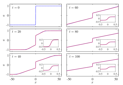
Figure 1: Numerical (solid, blue) and asymptotic (dashed, red) solutions of the initial value problem for eq. (1) with initial data eq. (8) where $\varepsilon=0.1$ and $A=1$.

III.1 The inner solution

To capture the inner solution, we introduce into eq. (1) the short space $\xi=x/\varepsilon$ and long time $T=\varepsilon t$ scalings of the independent variables $x$ and $t$

$$\varepsilon u_{T}+\frac{1}{\varepsilon}uu_{\xi}=\frac{1}{\varepsilon}u_{\xi\xi T}.$$ (9)

Expanding the dependent variable

$$u=u_{0}(\xi,T)+\varepsilon u_{1}(\xi,T)+\dots,$$ (10)

and substituting this ansatz into (9) yields the leading order equation

$$u_{0}\partial_{\xi}u_{0}=\partial_{\xi\xi T}u_{0}.$$

This equation admits separated solutions $u_{0}(\xi,T)=f(\xi)a(T)$, leading to

$$ff^{\prime}a^{2}=f^{\prime\prime}\dot{a},$$

where ^′, $\dot{\ }$ denote derivatives with respect to $\xi$ and $T$, respectively. Introducing a separation constant $K>0$

$$\frac{\dot{a}}{a^{2}}=\frac{ff^{\prime}}{f^{\prime\prime}}=-K,$$

we obtain the solution

$$a(T)=\frac{a_{0}}{1+a_{0}KT},$$

and

$$f(\xi)=\sqrt{c}\tanh\left(\frac{\sqrt{c}}{2K}(\xi-\xi_{0})\right).$$

In these formulas, $K,a_{0},c$ and $\xi_{0}$ are arbitrary constants. To agree with the initial data (8), we set $c=1,K=\frac{1}{2},a_{0}=A,$ and $\xi_{0}=0.$ Thus, the leading order inner solution is

$$u\sim u_{in}(\xi,T)=\frac{A}{1+{\textstyle{1\over 2}}AT}\tanh\xi.$$ (11)

The inner solution reveals the smoothed structure of the dispersively regularised expansion shock and its algebraic temporal decay.

III.2 The outer solution

The outer solution has a different, long space and time scaling

$$X=\varepsilon x,\quad T=\varepsilon t.$$

This leads to the scaled equation

$$\varepsilon u_{T}+\varepsilon uu_{X}=\varepsilon^{3}u_{XXT}.$$ (12)

With the expansion $u(X,T)=\tilde{u}_{0}(X,T)+\varepsilon\tilde{u}_{1}(X,T)+\cdots$, we have the leading order conservation law

$$\partial_{T}\tilde{u}_{0}+\tilde{u}_{0}\partial_{X}\tilde{u}_{0}=0.$$

We write the general, implicit solution by characteristics in the form

$$\tilde{u}_{0}(X,T)=f(T-\frac{X}{\tilde{u}_{0}}).$$

Matching to the inner solution, we have, for $x>0,$

$$\lim_{X\to 0+}\tilde{u}_{0}(X,T)=f(T)=\lim_{\xi\to\infty}u_{0}(\xi,T)=\frac{A}{1+{\textstyle{1\over 2}}AT}.$$

The matching for $x<0$ is similar, giving an odd function for the outer solution.

$$\tilde{u}_{0}=\frac{A\,\mathrm{sgn}(X)}{1+{\textstyle{1\over 2}}A(T-\frac{X}{\tilde{u}_{0}})}.$$

Solving for $\tilde{u}_{0}$, we find the leading order outer solution

$$u\sim u_{out}(X,T)=\frac{A({\textstyle{1\over 2}}X+\mathrm{sgn}(X))}{1+{\textstyle{1\over 2}}AT},\quad|X|<AT.$$ (13)

Continuous matching to the constant, far field conditions we obtain

$$u_{out}(X,T)=\mathrm{sgn}(X)A,\quad|X|\geq AT.$$ (14)

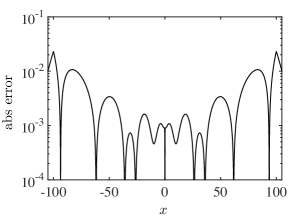
Figure 2: Pointwise error between the uniform asymptotic expansion and numerical solution of Fig. 1 at $t=100$ with $\varepsilon=0.1$, and $A=1$.

III.3 Uniformly valid asymptotic solution

Using the standard technique from asymptotics, we can formulate a composite solution that is asymptotically valid over the entire range of $x$. Based on the outer solution (13), (14), we define

$$F(x,t,\varepsilon)=\left\{\begin{array}[]{ll}-A,&x<-At\\[6.0pt] \displaystyle\frac{A({\textstyle{1\over 2}}\varepsilon x+\mathrm{sgn}(\varepsilon x))}{1+{\textstyle{1\over 2}}A\varepsilon t},&|x|<At\\[6.0pt] A,&x>At\end{array}\right.$$

Then the uniformly valid asymptotic solution is

$$u(x,t)=\frac{A}{1+{\textstyle{1\over 2}}A\varepsilon t}\left(\tanh\frac{x}{\varepsilon}-\mathrm{sgn}(x)\right)+F(x,t,\varepsilon).$$ (15)

A comparison of the uniform asymptotic expansion to the numerical solution is shown in Fig. 1. The two solutions are hardly distinguishable. The insets of Fig. 1 reveal the smoothed, non-oscillatory nature of the dispersively regularised expansion shock. In contrast, typical dispersive shock waves are characterised by their oscillatory structure el_dsws_2016 . Figure 2 displays the absolute error. Note that the largest error occurs at the outermost edges of the rarefaction wave where the asymptotic solution has a weak discontinuity. The error in the inner solution is approximately $\varepsilon^{3}=10^{-3}$, which can be formally identified by going to higher order terms in eq. (9). In Fig. 3(b) we show characteristics calculated from the outer solution (13), (14) with $\varepsilon=0.1$ and $A=1$.

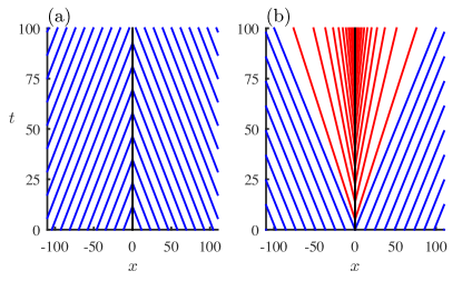
Figure 3: Characteristics for: (a) the compressive shock solution of equation (5); (b) the expansion shock solution of equation (1).

III.4 Boussinesq equations

The Boussinesq equations, formulated in the 1870s boussinesq , can take a variety of asymptotically equivalent forms whitham_linear_1974 . While having the same level of accuracy as the KdV and BBM equations in reproducing dispersive shallow water dynamics, the Boussinesq equations have the advantage of bi-directionality. The system considered here

$$\begin{array}[]{rcl}h_{t}+(uh)_{x}&=&0\\[6.0pt] u_{t}+uu_{x}+h_{x}-{\textstyle{1\over 3}}u_{xxt}&=&0,\end{array}$$ (16)

is a reduced, normalised version of an equation that appeared in whitham_linear_1974 (see also bona ), which includes a $u_{x}$ term in the dynamical equation for $h$. The non-dimensional variables $h,u$ represent the height of the water free surface above a flat horizontal bottom, and the depth-averaged horizontal component of the water velocity, respectively. A stationary shock solution of this system

$$h(x,t)=\left\{\begin{array}[]{ll}h_{-},&x<0\\[6.0pt] h_{+},&x>0,\end{array}\right.u(x,t)=\left\{\begin{array}[]{ll}u_{-},&x<0\\[6.0pt] u_{+},&x>0,\end{array}\right.$$ (17)

will satisfy Rankine-Hugoniot (RH) jump conditions derived from the time-independent equations,

$$h_{+}u_{+}=h_{-}u_{-};\ \ h_{+}+{\textstyle{1\over 2}}u_{+}^{2}=h_{-}+{\textstyle{1\over 2}}u_{-}^{2}.$$ (18)

The RH conditions (18) are attained for the two-parameter loci of states

$$u_{\pm}=h_{\mp}\left(\frac{2}{h_{-}+h_{+}}\right)^{1/2},$$ (19)

with arbitrary, positive total water depths $h_{\pm}$. In Fig. 4, we show the result of a numerical simulation demonstrating the persistence of a stationary shock wave for the Boussinesq system (16).

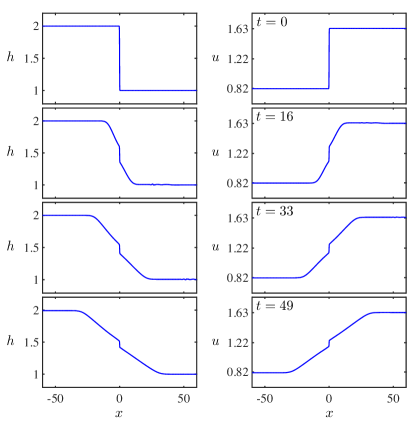
Figure 4: Evolution of $h$ (left) and $u$ (right) in an expansion shock for the Boussinesq system with $h_{-}=2$, $h_{+}=1$ and $u_{-}$, $u_{+}$ given by eq. (19). Jump initial data is smoothed by $\tanh(x/\varepsilon),$ as in eq. (8), with $\varepsilon=0.1.$

The characteristic speeds for the dispersionless system ((16) with $u_{xxt}\to 0$) are $\lambda_{\pm}(h,u)=u\pm\sqrt{h}.$ Therefore, if $u_{\pm}\geq 0$ as in the loci (19), then the characteristics with speed $\lambda_{+}$ pass through the stationary shock from left to right. However, the characteristics with speed $\lambda_{-}$ leave the shock on both sides if $u_{-}<\sqrt{h_{-}}$ and $u_{+}>\sqrt{h_{+}}.$ This is the case for the choices of $h_{\pm},u_{\pm}$ in Fig. 4. These choices also satisfy the Rankine-Hugoniot conditions for a stationary shock (18). To see that similar data with $u<0$ can make a stationary shock expansive in the $\lambda_{+}$ characteristic family, note that the system (16) is unchanged under the transformation $x\to-x$, $u\to-u$.

We remark that the analytical treatment of the Boussinesq expansion shock appears to be more challenging than it was for BBM. For example, there is no clear means to separate variables in an inner solution due to the nonzero mean values of $h$ and $u$.

III.5 Discussion

The expansion shock solutions we have discovered here do decay slowly in time, but their persistence in the face of the usual rules of causality is a surprise. For the BBM expansion shock, we can identify further robustness to perturbation by considering the asymmetric initial condition passing through zero

$$u(x,0)={\textstyle{1\over 2}}\left((u_{+}-u_{-})\tanh(\frac{x}{\varepsilon})+u_{+}+u_{-}\right),$$

where $u_{-}<0<u_{+}$. The numerical simulation of eq. (1) with this asymmetric data is shown in Fig. 5. As $t$ increases, the solution quickly develops a stationary, expansion shock with initial amplitude $A=\min\{u_{+},|u_{-}|\}$, that decays according to the inner solution (11). However, the solution also sheds a train of rank ordered solitons.

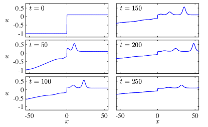
Figure 5: Expansion shock and solitons as components of the initial value problem $u(x,0)=0.55\mathrm{tanh}(x/\varepsilon)-0.45$ for eq. (1) where $\varepsilon=0.1$.

The expansion shock also persists in the presence of weak dissipation in the BBM-Burger’s equation

$$u_{t}+uu_{x}=u_{xxt}+\nu u_{xx},$$ (20)

where $\nu>0$ is the dissipation coefficient. If we consider the initial data (8) for (20), then the inner solution exhibits exponential temporal decay

$$u_{in}(\xi,T)=\frac{Ae^{-\nu T/\varepsilon}}{1+\frac{A\varepsilon}{2\nu}(1-e^{-\nu T/\varepsilon})}\tanh\xi.$$ (21)

Thus, for $\nu=\mathcal{O}(\varepsilon)$, the expansion shock decays exponentially as $t\to\infty,$ rather than the algebraic decay in the absence of diffusion. In fact, if $\nu\ll\varepsilon$, then (21) is asymptotically equivalent to (11).

The construction presented here can be generalised to higher order nonlinearity $f(u)$ and higher order, positive differential operators $\mathcal{L}$ in the form

$$\begin{split}\mathcal{L}[u_{t}]+f(u)_{x}&=\nu u_{xx},\end{split}$$ (22)

so long as the non-evolutionary, dispersive character is maintained. For example, $\mathcal{L}=1-\partial_{xx}$ and $f(u)=u^{4}$ or $\mathcal{L}=1+\partial_{xxxx}$ and $f(u)=u^{2}$ admit expansion shock solutions that can be approximated with matched asymptotic methods.

Recalling that the original formulation of the BBM equation (1) was as a numerically advantageous shallow water wave model, peregrine_calculations_1966 , it is important to stress that “engineering” the dispersion for mathematical or numerical convenience can lead to new, unintended phenomena, e.g., expansion shocks.

III.6 Conclusions

We have identified decaying expansion shocks as robust solutions to conservation laws of non-evolutionary type that naturally arise in shallow water theory. These models include versions of the well-known BBM and Boussinesq equations, which are weakly nonlinear models for uni-directional and bi-directional long wave propagation, respectively, although as written here, they are not asymptotically resolved. The requisite non-local dispersion in these models is not peculiar to shallow water theory, occurring, for example, in a Buckley-Leverett equation with dynamic capillary pressure law, hassanizadeh1990 describing flow in a porous medium. Expansion shocks represent a new class of purely dispersive and diffusive-dispersive shock waves. An important open question is whether expansion shock solutions can be physically realised.

This work was supported by the Royal Society International Exchanges Scheme IE131353 (all authors), NSF CAREER DMS-1255422 (MAH), and NSF DMS-1517291 (MS).

Appendix A Numerical Method

The numerical methods utilised here for both the BBM (1) and Boussinesq (16) equations incorporate a standard fourth order Runge-Kutta timestepper (RK4) and a pseudospectral Fourier spatial discretisation, similar to the method described in el_dispersive_2015 . We briefly describe the method for BBM here.

We are interested in solutions $u(x,t)$ to (1) that rapidly decay to the far field boundary conditions $u(\pm\infty,t)=u_{\pm}$. The derivative $v=u_{x}$ therefore rapidly decays to zero and satisfies

$$(1-\partial_{xx})v_{t}+(uv)_{x}=0,$$ (23)

where $u(x,t)=\int_{-L}^{x}v(y,t)\,\mathrm{d}y+u_{-}$. The Fourier transform (written $\widehat{f}(k)$ with wavenumber $k$ for a function $f(x)$) of eq. (23) can therefore be written

$$\frac{\mathrm{d}}{\mathrm{d}t}\widehat{v}=-\frac{ik}{1+k^{2}}\widehat{uv}.$$ (24)

The term $\widehat{uv}$ is well-defined because the function $uv$ is rapidly decaying. Suitable truncation of the spatial and Fourier domains turn eq. (24) into a nonlinear system of ordinary differential equations, which we temporally evolve according to RK4. The computation of the nonlinear term in (24) is efficiently implemented using the fast Fourier transform (see el_dispersive_2015 for further details). For BBM, $(L,N,\Delta t)=(200,2^{15},0.01)$ (Figs. 1, 2), $(300,2^{15},0.01)$ (Fig. 5). For Boussinesq, $(L,N,\Delta t)=(100,2^{14},0.005)$.

References

- (1) Peregrine DH. Calculations of the development of an undular bore. J Fluid Mech. 1966;25(2):321–330.
- (2) Benjamin TB, Bona JL, Mahony JJ. Model equations for long waves in nonlinear dispersive systems. Phil Trans Roy Soc London A. 1972;272(1220):47–78.
- (3) Whitham GB. Linear and nonlinear waves. New York: Wiley; 1974.
- (4) Johnson RS. Camassa–Holm, Kortweg–de Vries and related models for water waves. J Fluid Mech. 2002;455:63–82.
- (5) Bona JL, Tzvetkov N. Sharp well-posedness results for the BBM equation. Discrete Contin Dyn Syst. 2009;23(4):1241–1252.
- (6) Colliander J, Keel M, Staffilani G, Takaoka H, Tao T. Sharp global well-posedness for KdV and modified KdV on and . J American Math Soc. 2003;16:705–749.
- (7) Chen G, Olver PJ. Dispersion of discontinuous periodic waves. Proc Roy Soc London A. 2012;469:20120407.
- (8) Whitham GB. Variational methods and application to water waves. Proc Roy Soc A. 1967;299:6–25.
- (9) Moldabayev D, Kalisch H, Dutykh D. The Whitham equation as a model for surface water waves. Physica D. 2015;309:99–107.
- (10) Gurevich AV, Pitaevskii LP. Nonstationary structure of a collisionless shock wave. Sov Phys JETP. 1974;38(2):291–297.
- (11) Fornberg B, Whitham GB. A numerical and theoretical study of certain nonlinear wave phenomena. Phil Trans Roy Soc A. 1978;289:373–404.
- (12) El GA, Hoefer MA, Shearer M. Dispersive and diffusive-dispersive shock waves for nonconvex conservation laws. arXiv:150101681 [nlinPS]. 2015;.
- (13) El GA, Hoefer MA. Dispersive shock waves and modulation theory. Physica D, to appear, preprint: arXiv:160206163 [nlinPS]. 2016;.
- (14) Lax PD. Hyperbolic systems of conservation laws II. Comm Pure Appl Math. 1957;10(4):537–566.
- (15) Boussinesq JV. Théorie générale des mouvements qui sont propagés dans un canal rectangulaire horizontal. C R Acad Sci Paris. 1871;73:256–260.
- (16) E SM. Existence of solutions for the Boussinesq system of equations. J Diff Eqns. 1981;42:325?352.
- (17) Mikhailov AV, Novikov VS, Wang JP. On Classification of Integrable Nonevolutionary Equations. Stud Appl Math. 2007;118(4):419–457.
- (18) Bona JL, Chen M, Saut JC. Boussinesq equations and other systems for small–amplitude long waves in nonlinear dispersive media. I: derivation and linear theory. J Nonlinear Sci. 2002;12:283–318.
- (19) Hassanizadeh SM, Gray WG. Mechanics and thermodynamics of multiphase flow in porous media including interphase boundaries. Adv Water Resour. 1990;13:169–186.