Status Report:
Searching for a Sterile Neutrino at J-PARC MLF (E56, JSNS2)
M. Harada, S. Hasegawa, Y. Kasugai, S. Meigo, K. Sakai,
S. Sakamoto, K. Suzuya
JAEA, Tokai, JAPAN
E. Iwai, T. Maruyama111Spokesperson:
(takasumi.maruyama@kek.jp) ,
S. Monjushiro, K. Nishikawa, M. Taira
KEK, Tsukuba, JAPAN
M. Niiyama
Department of Physics, Kyoto University, JAPAN
S. Ajimura, T. Hiraiwa, T. Nakano, M. Nomachi, T. Shima
RCNP, Osaka University, JAPAN
T. J. C. Bezerra, E. Chauveau, H. Furuta, F. Suekane
Research Center for Neutrino Science, Tohoku University, JAPAN
I. Stancu
University of Alabama, Tuscaloosa, AL 35487, USA
M. Yeh
Brookhaven National Laboratory, Upton, NY 11973-5000, USA
W. Toki
Colorado State University, Fort Collins, Colorado, USA
H. Ray
University of Florida, Gainesville, FL 32611, USA
G. T. Garvey, C. Mauger, W. C. Louis, G. B. Mills, R. Van de Water
Los Alamos National Laboratory, Los Alamos, NM 87545, USA
J. Spitz
University of Michigan, Ann Arbor, MI 48109, USA
1 Introduction
The JSNS2 (J-PARC E56) experiment aims to search for sterile neutrinos at the J-PARC Materials and Life Sciences Experimental Facility (MLF). After the submission of a proposal [1] to the J-PARC PAC, stage-1 approval was granted to the JSNS2 experiment. The approval followed a series of background measurements which were performed in 2014 [2].
Subsequent for stage-1 approval, the JSNS2 collaboration has made continuous efforts to write a Technical Design Report (TDR). This TDR will include two major items as discussed in the previous status report for the 20th J-PARC PAC [3]:
-
•
A realistic detector location
-
•
Well understood and realistic detector performance using simulation studies, primarily in consideration of fast neutron rejection.
Since August we have been in discussions with MLF staff regarding an appropriate detector location. We are also in the process of setting up a Monte Carlo (MC) simulation framework in order to study detector’s performance in realistic conditions. In addition, we have pursued hardware RD work for the liquid scintillator (LS) and to improve the dynamic range of the 10” photomultiplier tubes (PMTs). The LS RD works includes Cherenkov studies inside the LS, and a Pulse Shape Discrimination (PSD) study with a test-beam, performed at Tohoku University. We also estimate the PSD performance of a full-sized detector using a detailed MC simulation.
In this status report, we describe progress on this work.
2 Discussion for the detector location with MLF
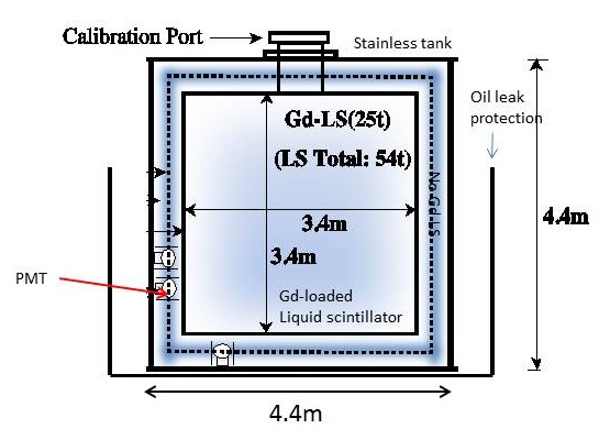
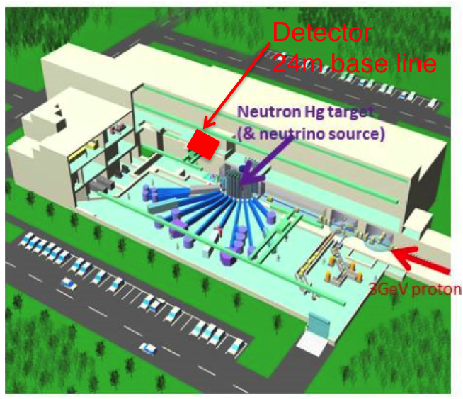
To maximize sterile neutrino sensitivity in the region of interest, it is optimal to put the JSNS2 detectors (Fig. 1) 24 meters from the MLF mercury target, as reported in Ref. [2]. This position is located in the “large component handling room”, the room to handle large equipment of the MLF, on the third floor in the MLF building (Fig. 2). The room is not a common experimental area, but is considered a maintenance work area for MLF operations. Therefore, in order to carry out the JSNS2 experiment, we need to discuss and understand the issues associated with this detector location. In addition, it is important to clarify the application of safety regulations for the JSNS2 detectors, which contains more than 100 tons of liquid scintillator.
In August, 2015, the JSNS2 collaboration requested the KEK IPNS director / the director of J-PARC center facilitate discussions between MLF and JSNS2, to address these issues in detail. Since that time we have held several meetings with directors, MLF, and the local fire department.
In the discussion, there are no show-stoppers that inhibit the JSNS2 experiment. The JSNS2 collaboration will try to realize the experiment with further discussions in detail in the TDR.
3 RD for the JSNS2 Detector
3.1 Cherenkov study with LAB+0.03g b-PBD
As described in the previous status report [3], we verified the performance of the liquid scintillator used in the LSND experiment, mineral oil plus 0.03 g/L b-PBD.
In this status report we investigate the performance of LAB + 0.03g/L b-PBD liquid scintillator since we plan to use the LAB in the JSNS2 experiment. We use the LSND 0.03 g/L b-PBD as a reference point for the LAB performance checks. The amount of secondary light emission materials such as b-PBD or PPO determine the light yield, and the type of material determines the light emission time, in addition to the LAB properties.
3.1.1 Setup of the Measurement
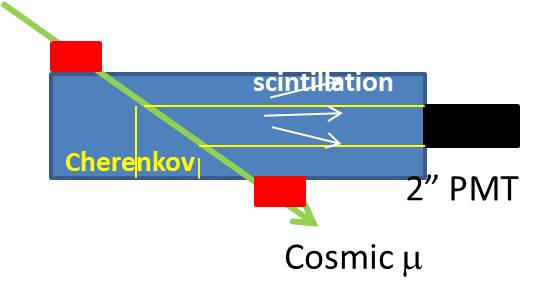
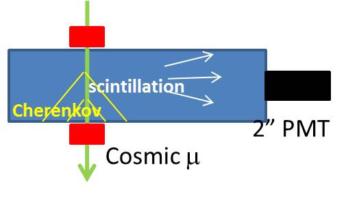
The setup and the data analysis of the measurement is exactly the same as that in the previous status report [3] (Fig. 3). The cylindrical prototype is filled with the liquid scintillator, and a black sheet is used to avoid reflections of light inside the cylinder. The motivation of this experiment is to mainly measure the timing difference between Cherenkov light and scintillation light. In general, the Cherenkov light has a faster emission time than that of the scintillation light.
3.1.2 Data Analysis and Results
Hit definition
Figure 4 shows a set of typical waveform timing distributions measured by a digital oscilloscope. We used the oscilloscope data for this analysis. The top plot shows typical timing distributions of the coincidence from the scintillation counters, and the middle and bottom plots show typical scintillation light signals, which corresponds to the signals with the setup of Fig. 3(b). For the explanation of the analysis, only the typical signals in Fig. 3(b) are described here. Note that the coincidence signal from the scintillation counters was delayed due to electronics. Also, this relative timing was smeared by the PMT’s jitter (1 ns), electronics (within 1 ns), and hit position of the cosmic rays ( ns). The fastest scintillation light or Cherenkov light should be located around 24980 time counts. This was demonstrated by using a Water Cherenkov setup [3].
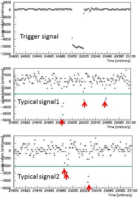
As shown in Fig. 4, there is a threshold to determine the timing of the “hit”, which is 2000 counts ( 1/3 p.e.) in the data. In the figure, thresholds correspond to the green lines, and the red arrows show the recognized hits above the thresholds. These typical signals have multiple hits.
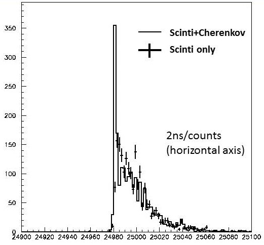
Results: Comparison between scintillation only and Cherenkov+scintillation light
Figure 5 shows the relative timing of hits with respect to the coincidence defined by the thresholds, and also shows the timing comparison between scintillation light only (cross) and Cherenkov + scintillation light (histogram). As clearly seen, Cherenkov light is concentrated in the fast timing peak. If we select the fastest timing in the first 2 ns bin, the 95 of scintillation light is rejected from Cherenkov light while only 25 of scintillation light is contaminated into the Cherenkov light.
An estimated light yield is 1600 photons/MeV. Compared to the 9000 photons/MeV measured by Daya Bay experiment [5], a dilution factor, which is defined as the ratio between the light yield of the nominal scintillator and that of the scintillator with small amount of the secondary light emission materials, is 5.3.
3.1.3 Simulation of the Measurement
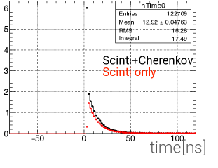
We also evaluated the results using a simulation to understand the optical properties of the medium. The software will be described later in Section 4. Figure 6 shows the timing distribution of single photoelectrons obtained with the Monte Carlo simulation before parameter tuning. We will continue to study the measurement results to tune the optical parameters precisely.
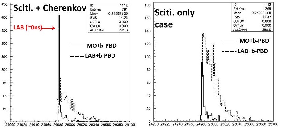
3.1.4 Results; Comparison between Mineral Oil and LAB
Finally, we compare the results of this study between mineral oil and LAB (Fig. 7). The following observations have been made: (A) Emission time of scintillation light with LAB+0.03 g/L b-PBD is wider than that in the mineral oil+0.03 g/L b-PBD. (B) Light yield in the LAB+0.03 g/L b-PBD is higher than that in the mineral oil+0.03 g/L b-PBD case by a factor of six. (C) The yield of the Cherenkov light is the same in the two liquid scintillators within 10.
3.2 Study of PSD capability with JSNS2 detector
As presented in the previous status report for the PAC [3], there are indications that the Daya Bay type of Gd-loaded liquid scintillator (DBLS) produces a strong PSD capability in the several MeV range. The PSD capability is crucial in rejecting cosmic induced fast neutrons by a factor of 100, and also important for keeping the neutrino detection efficiency as high as possible. However, the measurements were done with a small vial detector and a less than 10 MeV source (252Cf neutron source). Therefore, it is important to show the feasibility in the actual energy range and full JSNS2 detector size. In order to demonstrate the PSD capability of the DBLS, a measurement using a 70 MeV neutron beam created by a cyclotron in the Cyclotron and Radioisotope Center (CYRIC) at Tohoku University was performed in October 2015. The current status of the MC study and first look plots of the neutron beam measurement are shown in this section. Another effort to evaluate the PSD capability with the real size detector was made using a realistic MC simulation. The PSD parameters were extracted from the vial test, and they were extrapolated to a real size detector. The results of this study are shown in the following sections.
3.2.1 MC study of PSD capability of the DBLS with a full size JSNS2 detector
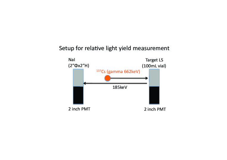
The PSD capability of the DBLS with a full size detector was calculated with a MC simulation based on Geant4 [6]. Each PSD related parameter (scintillation light yield, the light emission time, Birks constant, etc.) of the DBLS was tuned by using measured data with a 100 mL cylindrical vial with an attached 2 inch PMT.
Figure 8 shows the setup for the measurement of light yield of the DBLS. To detect backscattering events which gamma rays are emitted from a 137Cs source and detected by the NaI detector via the Compton scatter in the DBLS detector, the 137Cs source is set between the DBLS and the NaI detectors as shown in Fig. 8. This setup allows us to detect only Compton edge events with scattered angle of 180 degrees. The coincidence signal from the DBLS and the NaI detectors is used as the trigger. The data are taken with a flash ADC module (CAEN V1730, 500 MS/s, 14 bits).
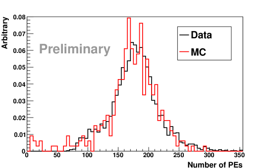
The black line in Fig. 9 shows the number of photoelectrons of the backscattering events. Comparing the peak of liquid scintillator of KamLAND experiment, with known light yield (8300 photons/MeV [7]), the relative light yield of the DBLS can be measured. Thus, the light yield is estimated as 10000 photons/MeV, compared to the 9000 photons/MeV measured by Daya Bay experiment [5]. The red line in Fig. 9 shows the MC distribution after implementing the measured light yield.
The black lines in Fig. 10 show the measured mean waveforms of gammas (left plot) and neutrons (right plot) from the 241Am9Be source with the vial. The time constants of the scintillation light emission in the MC simulation were calculated by fitting the mean waveform data by the expectation, summing 3 exponentials in consideration of the mean waveform of one photoelectron and TTS of the 2 inch PMT. Table 1 shows each parameter of the fit result, and filled areas in Fig. 10 show the expected waveform of each time constant of the fit result.
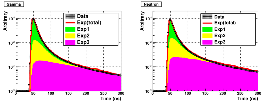
| Component | time constant | ratio (gamma) | ratio (neutron) |
|---|---|---|---|
| Exp1 | 3.87ns | 0.673 | 0.580 |
| Exp2 | 17.6ns | 0.187 | 0.219 |
| Exp3 | 148.3ns | 0.140 | 0.200 |
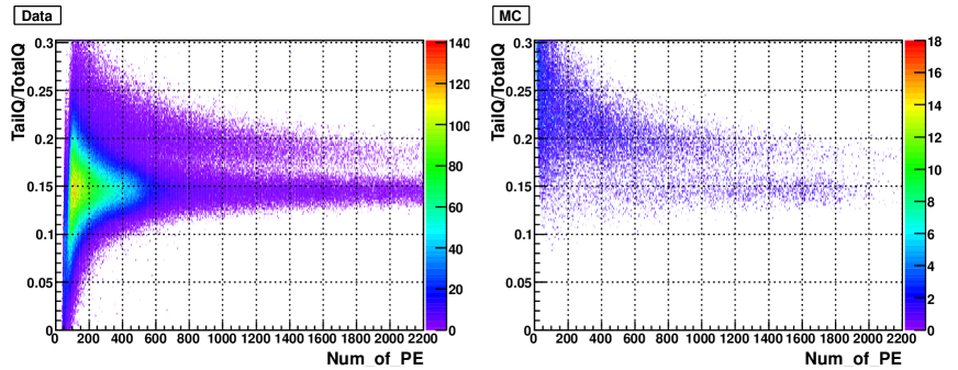
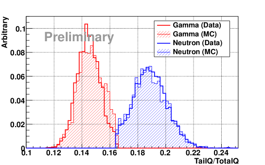
Figure 11 shows the TailQ/TotalQ variable, whose definition is the same as the previous PAC report [3], as a function of the detected number of photoelectrons for the DBLS. The left plot shows data with the 241Am9Be source, including background such as environmental gammas in particular, and the right plot shows the MC with only the 241Am9Be source. Although there is a discrepancy due to the environmental gammas in the range below 600 photoelectrons, the MC reproduces the data well in the high photoelectron range. Figure 12 shows the TailQ/TotalQ distributions of events between 1000 and 2000 photoelectrons. Both the gamma and neutron data are well reproduced by the MC.
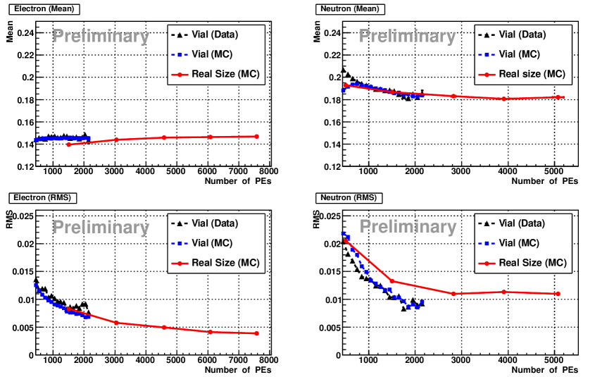
Using the MC simulation with the tuned parameters mentioned above, the PSD capability of the DBLS with the realistic JSNS2 detector was evaluated. To check the PSD capability in the several tens of MeV range of the prompt signals, electrons and neutrons with various energies between 10 and 50 MeV were generated at the JSNS2 detector center. The upper figures in Fig. 13 show the means of the TailQ/TotalQ distributions as a function of the detected number of photoelectrons for the electrons (left) and neutron-induced proton recoils (right). The lower plots show the RMS. The blue and black markers show the data and MC of the vial measurement with 241Am9Be source, respectively, and the red lines show MC results with the JSNS2 detector. The vial measurement data are well reproduced by the MC in all plots, and extrapolation curves of the MC with the JSNS2 detector (red lines) from the lower photoelectron range of the vial measurement looks reasonable, except for the case of RMS of protons recoiled from neutrons (bottom right plot). The MC with the JSNS2 detector is working well. The reason of the discrepancy of the RMS curve of the recoiled protons is likely due to a geometrical effect; an investigation into this discrepancy is on-going.
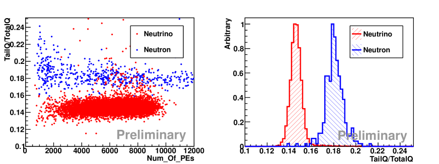
The left plot in Fig. 14 shows MC results of the correlations between means of the TailQ/TotalQ distributions and the detected number of photoelectrons due to 100% oscillated neutrino signals (red) and protons from cosmic induced fast neutron interactions (blue) generated using the same method as the proposal for JSNS2 [1]. The right plot shows the TailQ/TotalQ distributions of the neutrinos and protons after applying a simplified neutrino selection criteria (20 Eprompt 60 MeV, 5 Edelayed 12 MeV, 0 t 100 sec, multiplicity of thermal neutron capture = 1). The red and blue colors in Fig. 14 show the neutrinos and recoiled protons, respectively. The plot shows good separation between the neutrinos and recoiled protons, due to neutron-proton elastic scattering. However, there is a possibility to include inelastic scattering or spallation with gammas between the neutrons and 12C in the scintillator. If there are such events with gammas, the neutron rejection power becomes worse compared to the MC result which includes only recoiled protons. Thus, it is important to check the PSD capability in the events with gammas caused by neutrons of several tens of MeV.
3.2.2 PSD capability with test-beam
To check the PSD capability in the prompt energy range and the inelastic or spallation events between the cosmic induced fast neutron and 12C in the scintillator, a measurement with a neutron beam of 70 MeV was carried out in CYRIC in Tohoku University. CYRIC has a high-intensity fast neutron facility [8]. A proton beam provided by the AVF cyclotron hits a Li target, producing the quasi-monoenergetic neutron beam from 14 to 80 MeV via the 7Li(p,n)7Be reaction. Figure 15 shows a schematic layout of the fast neutron beam facility. The DBLS with the 100 mL vial with an attached 2 inch PMT is set on the beam axis at the facility. Two cylindrical NaI counters (2” (diameter) 2” (height) and 3” (diameter) 3” (height)) were also set on both sides of the DBLS for checking the events following gammas due to the inelastic or spallation reaction of 12C.
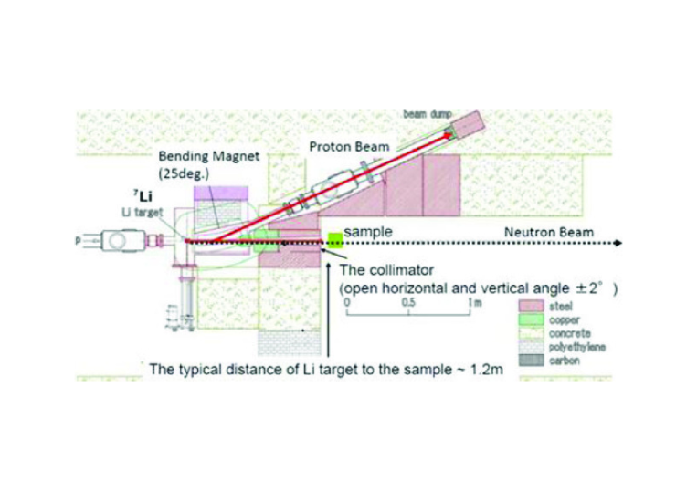
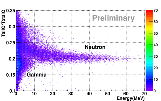
Figure 16 shows a first look plot of the correlation between the TailQ/TotalQ variable and the detected number of photoelectrons of the DBLS. The band due to the neutron events can be confirmed in the higher TailQ/TotalQ range. The detailed analysis is ongoing; results will be presented in the next PAC report.
3.3 Dynamic range of the PMT
JSNS2 is planning to use 150 10-inch photomultiplier tubes (PMTs). A candidate PMT is R7081 of Hamamatsu Photonics, which is used in the Double Chooz and RENO reactor experiments. The main difference of JSNS2 from Double Chooz or RENO is the light yield. For the case of JSNS2, the maximum neutrino energy is MeV, 10 times higher than that of typical reactor neutrinos. The liquid scintillator is contained in an acrylic vessel and the PMTs will be submerged in non-Gd loaded scintillator outside the acrylic vessel. If a neutrino signal happens in the liquid scintillator just in front of a PMT, the PMT shall receive scintillation light as high as 1,000 p.e. equivalent. On the other hand, the lowest signal energy to detect is a few MeV and if such event happens far from a PMT, the PMT shall receive 1 p.e. or less. Since JSNS2 will perform the spectrum analysis of the neutrino signal to separate the intrinsic background from decay at rest, the PMT must have a linear dynamic range from 1 p.e. to 1,000 p.e.
To obtain such large dynamic range, we will use a tapered base circuit as shown in Fig. 17.
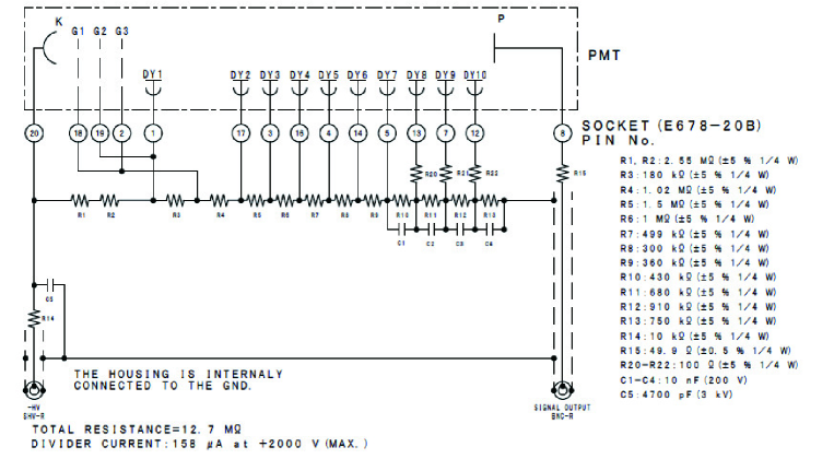
The voltage bias between dynodes is set higher for latter dynodes to reduce the space charge effect. The linearity of the gain was measured by using 7 liter liquid scintillator and 8 inch PMT as shown in Fig. 18.
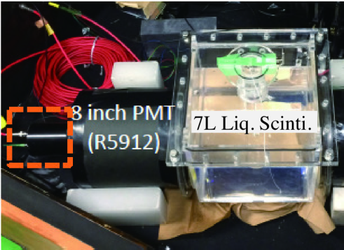
For the test, the liquid scintillator was contained in an UV-transparent acrylic vessel that was readout by an 8 inch PMT. Two base circuits, one as the regular divider and the other as the tapered divider, were prepared and the base sockets were swapped to compare the measurement results. A 500 MHz, 14bit flash ADC (CAEN V1730) was used to readout the pulse shape.
At first, one p.e. peak was measured by using a triggered LED to obtain the absolute gain. The gain of the PMT was set to for a 1 p.e. signal. The cosmic-ray signal was measured to obtain the large amplitude signals. A saturation effect was measured using the ratio of the output charge (Q) and pulse height (H), which is a good indicator of the non-linearity of the gain.
Figures. 19(a) and (b) show the Q/H ratio which indicates that, for the tapered circuit, the ratio is almost stable up to 1,000 p.e. while for the regular circuit, the ratio changes from 300 p.e.
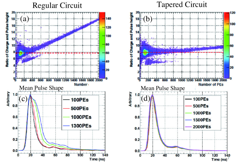
Figure 19, (c) and (d), shows how the pulse shape changes depending on the input charge. For the PMT with the tapered base circuit, the shape does not change up to 1,000 p.e., which is important for the pulse shape discrimination analysis.
4 Software efforts to show the fast neutron rejection
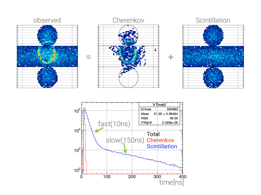
At present, the most pressing issue in the JSNS2 design is identifying and rejecting background fast neutron events when selecting signal neutrinos. Cosmic-induced neutrons, rather than beam-induced neutrons, are the primary concern. PSD and Cherenkov light can be used to differentiate the two classes of events. However, this rejection is strongly dependent on a number of variables, including: liquid scintillator properties, photo-coverage, light detection technology, tank geometry, veto layer(s), electronics response, dynamic range, and timing resolution, among others. These JSNS2 detector design considerations are studied, in part, with a dedicated simulation package based on Geant4 [6]. An example event display is shown in Fig. 20 along with the timing characteristics of the event. The figure shows a simulated 50 MeV positron in the JSNS2 cylindrical volume with the dilution factor of 10 for scintillation light. The Cherenkov ring and scintillation light components can be easily seen.
The simulation is tuned and validated using data taken in a number of test stands at KEK and Tohoku University. For example, Fig. 6 shows the results of the simulation as compared to the KEK test stand (Fig. 5) in consideration of Cherenkov and scintillation light. Another aspect of the simulation involves studying PSD for separating neutron-induced proton and nuclear recoil events from positron-like events. This discrimination is based on the shape of the waveform. Neutron-induced event waveforms tend to have a larger tail and smaller peak amplitude than positron events. Data from the test stand at Tohoku University (See Section 3.2 for more details), featuring small volumes of liquid scintillator and a 241Am9Be and neutron source, are used to develop and tune a simulation of the interactions inside liquid scintillator as well as the PMT and electronics response in simulating waveforms properly. Figure 13 shows a Monte Carlo and data comparison for the few-MeV gamma (electron) and neutrons. Also shown is the Monte Carlo expectation for the pulse shapes all the way up to 50 MeV, which is most relevant for JSNS2. As can be seen, pulse shape discrimination becomes more powerful for higher energy species.
The ability to differentiate neutron-induced events from positrons appears to be quite promising using both Cherenkov-scintillation and pulse shape discrimination techniques. The software simulations continue to be expanded in scope and tuned to existing data. The 70 MeV neutron beam test data with the Tokoku University liquid scintillator volumes will allow the simulation to be further tuned and enhanced at energies most representative for JSNS2.
Reconstruction software work is also ongoing concurrently with the simulation efforts. The event vertex determination is based on a maximum likelihood algorithm using charge and time information. Both a point source event and an extended distribution can be considered when forming the event likelihood. The reconstructed energy is determined based on the number of photoelectrons, timing, and the vertex determination from the likelihood algorithm above. Optimizing the reconstruction, which is highly dependent on (e.g) non-linearities, light sensor properties, and liquid scintillator properties, involves working closely with the simulation software as well.
5 Summary and Plan
The JSNS2 collaboration is making continuous progress to produce a TDR.
For the detector location, there were many intensive discussions between the MLF and the JSNS2, on the safety requirements for the treatment of more than 100 tons of liquid scintillator, the interference between areas for the irradiated materials storage and operation of liquid scintillator, the weight load on the MLF building due to the detectors, leakage protection and the safety of the liquid scintillators, slow monitor and controls, ground sinkage of the MLF building due to the weight of the detectors, and procedures for bringing the detectors outside of the building. This interim report will be presented to the PAC, and further investigation will be done to produce the TDR.
JSNS2 detector RD has also made excellent progress. For the rejection of fast neutron events two methods are under study. One is using Cherenkov light and the other is using PSD. For the Cherenkov light technique, we checked the performance of the liquid scintillator made by LAB+0.03 g/L b-PBD. This liquid scintillator has excellent properties compared to the liquid scintillator comprising mineral oil plus 0.03 g/L b-PBD, in consideration of the light emission time for distinguishing between Cherenkov and scintillation light. For the method using PSD, we employed a test-beam using beam fast neutrons at Tohoku University. The analysis is on-going. The dynamic range of the 10” PMT was improved by more than three times due to the change of a register chain of the PMT base circuit. This improvement allows JSNS2 to have a good energy resolution up to 50 MeV.
In order to transform this RD information into the detector performance of the JSNS2, a software framework has been set up using Geant4. The data of the Cherenkov test using the prototype is reasonably reproduced by Geant4. The PSD performance for the neutron-proton elastic events in the real size detector was estimated using the simulation. These are also on-going efforts.
In summary, the continued JSNS2 progress indicates the TDR will be produced on schedule, within about one year from now.
6 Acknowledgements
We warmly thank the MLF people, especially, Dr. Futakawa, J-PARC sub-director and Prof. Kanaya, MLF Division leader, the neutron source group, muon group and the user facility group for their support. For the discussion between the MLF and the JSNS2 experiment, we appreciate the help from Katsuo Tokushuku (KEK IPNS director), Naohito Saito (J-PARC director), Tetsuro Ishii (J-PARC sub-director), Takashi Kobayashi (KEK IPNS sub-director) and the J-PARC safety Division in addition to the MLF people mentioned above to set up constructive discussions.
Finally, we also acknowledge the support from grant-in-aid, J-PARC and KEK.
Appendix A Additional Physics Study under Consideration
A.1 Physics with neutrinos from charged kaon decay-at-rest
JSNS2 has the unique ability to precisely measure monoenergetic 236 MeV neutrinos from charged kaon decay-at-rest (; BR=63.5% [9]) for the first time. These neutrinos represent (1) an unprecedented weak-interaction-only, known energy probe of the nucleus, (2) a standard candle for developing a thorough understanding of the neutrino interaction and cross sections critical for future long baseline neutrino experiments, and (3) a source for a sterile neutrino search using electron neutrino appearance [10, 11]. These neutrinos have also been cited as important for probing muon neutrino disappearance at short baseline [12] and as a possible dark matter annihilation signature [13].
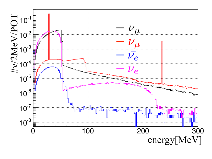
Despite the importance of the kaon decay-at-rest (KDAR) neutrino across multiple aspects of particle and nuclear physics, these neutrinos have never been studied or even identified before. The decay-in-flight neutrino “background” in conventional beamlines drowns out the KDAR signal in such experiments. Decay-at-rest sources of neutrinos, most notably spallation neutron sources, are excellent locations for studying KDAR due to their minimal decay-in-flight background and intense beams. However, the historically most intense spallation sources have been too low energy to produce kaons readily. The J-PARC MLF 3 GeV primary proton energy is sufficient to produce kaons efficiently and, also in consideration of the facility’s beam intensity (eventually 1 MW, currently 500 kW [14]), represents the best facility in the world to accomplish this physics. The KDAR neutrino can easily be seen in Fig. 21, which shows the neutrino flux at the J-PARC MLF source.
JSNS2 expects to collect a sample of between 150,000 and 300,000 charged current events in 50 tons of fiducial volume in its 5 year run222 The large variation in the expected number of events is due to the highly uncertain kaon production at this energy. The lower and upper bounds come from Geant4 [6] and MARS [15] predictions, respectively.. These events ( or ) are easily identifiable due to the characteristic double coincident signal of the prompt muon plus proton(s)/nucleus followed by the muon decay electron () a few later.
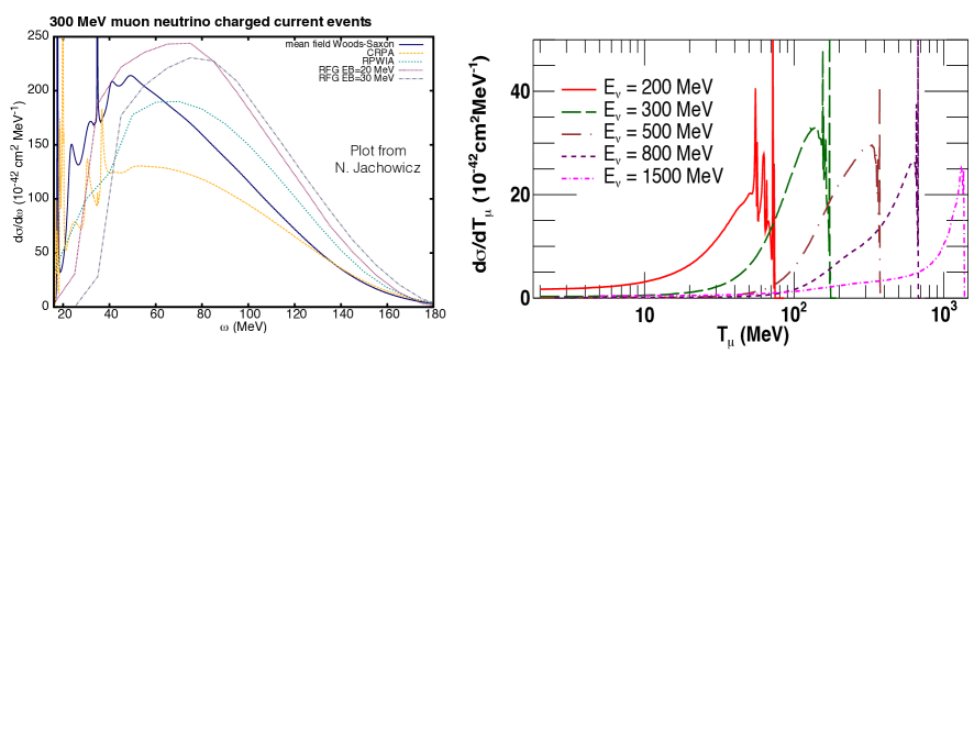
The known energy KDAR neutrinos provide the exclusive tool, for the first time, to study nuclear structure and the axial vector component of the interaction using electron scattering variables such as (). The importance of this unique access to the nucleus is potentially far-reaching. For example, a double differential cross section measurement in terms of vs. allows one to distinguish effects of the form factors, which depend only on , and of the nuclear model, which depends on both. Figure 22 (left) shows a number of model predictions for the differential cross section in terms of energy transfer for 300 MeV CC scattering on carbon. The disagreement between the models, in terms of both shape and normalization, is striking. Notably, the JSNS2 muon energy resolution may allow the nuclear resonances, easily seen in Fig. 22 (right), to be measured via neutrino scattering. The KDAR neutrino is likely the only way to study these excitations with neutrino scattering and, in general, to validate/refute these models in the MeV neutrino energy range (see, e.g., Ref. [16]).
Along with studying nuclear physics relevant for future neutrino experiments, the large sample of KDAR muon neutrinos collected with JSNS2 will provide a standard candle for understanding the neutrino energy reconstruction and outgoing lepton kinematics in the 100s-of-MeV neutrino energy region. While the KDAR neutrino is simply not relevant for experiments featuring significantly higher neutrino energies, most notably for MINOS, NOvA and DUNE [17, 18, 19], it is highly relevant for experiments with a large or majority fraction of few-hundred-MeV neutrinos, for example, T2K [20], MOMENT [21], the European Spallation Source Neutrino Super Beam (ESSSB) [22], and a CERN-SPL-based neutrino beam CP search [23]. In particular, MOMENT and ESSSB both feature spectra which peak at about 200-250 MeV.
The KDAR neutrino can also be used to search for electron neutrino appearance () for providing a probe of the sterile neutrino that will be highly complementary to the JSNS2 IBD search (). The advantage of the KDAR technique over other sterile neutrino searches is that the signal energy (236 MeV) is known exactly. A background measurement on either side of the signal energy window around 236 MeV can allow an interpolated determination of the expected background in the signal region with high precision. However, as compared to CC interactions, events ( or or ) are more challenging to identify over background, since they do not feature a double coincidence signal. While the KDAR events are expected to be distinct, in the sense that their reconstructed energy will lie close to 236 MeV, beam-induced neutrons can interact inside of the detector to produce an energetic single flash of light (e.g. a proton), mimicking a 236 MeV event. Pulse shape discrimination and particle identification via Cherenkov light can be used to mitigate this background, but the background event rate expectation remains significant. This is worrisome because the oscillated signal expectation is events in consideration of the global best fit region at high-. The possibility of probing appearance using KDAR neutrinos at the MLF remains an intriguing possibility, however, especially given strong Cherenkov-scintillation separation, pulse shape discrimination, and/or additional shielding.
The KDAR neutrino opens up new avenues for research in neutrino oscillation, interaction, and nuclear physics, and the importance of these measurements is clear. Perhaps most intriguing, the nucleus has simply never been studied using a known energy, weak-interaction-only probe and KDAR provides the exclusive technique to explore this frontier. JSNS2 represents the world’s best hope to take advantage of the KDAR neutrino in the near future. Other existing facilities worldwide simply cannot match the large expected KDAR signal and small expected decay-in-flight background rate at the J-PARC MLF.
A.2 Measurement of neutrino-induced nuclear reaction cross sections
A.2.1 Physics Motivations
Stars with initial masses greater than 810 times the solar mass are expected to end their lives with core collapsing supernova explosions (Type-II SNe). When such a massive star exhausts its nuclear fuel at the center, it produces no more heat to sustain its own weight, and materials in the outer layers begin to fall into the central core. The density and the temperature of the core rapidly increases, and the core is photo-dissociated to a mixture of nucleons and light nuclei, which absorb free electrons by emitting neutrinos. Finally, a proto-neutron star is formed. The core becomes so hard that the falling materials are repelled at the surface of the core. The repelled matter collides with the subsequently falling matter, generating an outgoing shockwave. It was found through a number of simulations on Type-II SNe within the spherically symmetric one-dimensional or two-dimensional models that the outgoing shockwave cannot get the kinetic energy of about 1051 erg which is necessary to propagate to infinity [26]. In order to solve the problem, many effects such as stellar rotation, the magnetic field and the neutrino-nucleus interactions have been studied [27], and now the delayed explosion model is considered as one of the promising and realistic models for Type-II SNe [28]. In this model, the kinetic energy needed for the explosion is considered to be supplied by the nuclear reactions between the matter in the shockwave and the neutrinos which carry almost 99 of the initial gravitational energy of the star, which is of the order of 1053 erg. From precise simulations of the dynamics of Type-II SNe, it was found that the neutrinos are trapped in the core, and are released after about a hundred milliseconds. Then they overtake the outgoing shockwave, supplying an additional kinetic energy via the neutrino-nucleus interactions. Since the region where the shockwave stalls is composed of light nuclei [29], the neutrino-induced nuclear reactions on light nuclei should play critical roles in the dynamics of explosions. From the one-dimensional and two-dimensional simulations for the explosion energy in Type-II SNe for different neutrino luminosities and fixed neutrino-nucleus reaction rates, it was found that the enhancement of the neutrino luminosity by 1015 leads to an increase of the order of 101051 erg/s in the explosion energy [30]. It suggests the enhancement of the neutrino-nucleus reaction rates with fixed neutrino luminosity also should give the same magnitude of increase in the explosion energy. Therefore the neutrino-nucleus reaction rates should be known with accuracy better than about 10 to evaluate the effect of neutrinos to the explosion.
Another important role of the neutrino-induced nuclear reactions concerns the r-process nucleosynthesis. A recent scenario of the r-process nucleosynthesis assumes the formation of the high-entropy neutron-rich gas, called the neutrino-driven wind, in the atmosphere of a nascent neutron star by the neutrino-induced spallation reactions, and the synthesis of heavy elements from protons and neutrons up to the nuclides with the mass number of 200250 within about one second [31, 32, 33]. This scenario is preferred, because it does not require the existence of the seed nuclei like iron, and naturally explains the universality of the r-elements, i.e. the similarity found in the r-element abundances in stars with different metallicities. More recently, it was pointed out that the neutrino-induced spallation reactions on light nuclei may efficiently produce lithium and boron in the oxygen/carbon layer of a Type-II supernova [34]. Such a process is interesting as a possible source of Li-Be-B in addition to the spallation by cosmic rays, and also as a new method to constrain the parameter of the flavor oscillation of the neutrinos. For more precise calculations, it is necessary to use accurate rates of the neutrino-induced nuclear reactions.
A.2.2 Current status of data for neutrino-induced nuclear reaction cross sections
So far, experimental data of the neutrino-induced nuclear reaction cross sections have been obtained by using neutrinos produced by accelerators or radioactive isotopes. Decay-at-rest (DAR) neutrinos from stopped pions and muons generated with high-energy accelerators are very useful for studies of the nuclear reactions induced by supernova (SN) neutrinos, because their energy spectra overlap with those of SN neutrinos as shown by Fig. 23.

Table 2 shows the list of the presently available experimental data for neutrino-induced nuclear reaction cross sections.
| Reaction | Neutrino Source | Accuracy | Reference |
|---|---|---|---|
| 12C(,eNg.s. | Accelerator | 10 | [35][36] |
| 12C(,eN∗ | Accelerator | 15 | [35][36] |
| 12C(,C | Accelerator | 20 | [35][36] |
| 13C(,eN | Accelerator | 76 | [35] |
| 56Fe(,eNi | Accelerator | 37 | [35] |
| 71Ga(,eGe | RI (51Cr) | 11 | [37][38] |
| 127I(,eXe | Accelerator | 33 | [39] |
As shown in Table 2, even in the case of the best studied 12C, the accuracy of the experimental data is not better than the one required in the SN simulations, and therefore new experimental data with better accuracy are still needed. JSNS2 is expected to provide an experimental opportunity to measure the neutrino-induced nuclear reaction cross sections with better accuracy due to a high-intensity neutrino beam from the J-PARC/MLF and a high-sensitivity/high-resolution detector system.
A.2.3 Plan for measurement of the neutrino-induced nuclear reaction cross sections in JSNS2 project
Background rejection and statistical accuracy
Assuming the neutrino flux of J-PARC/MLF to be
1.61014 /cm2/y/MW, one needs the number
of the target nucleus of at least 1029 atoms or the target
quantity of more than a few tons to measure the cross section in the
range of about 10-41 cm2 with a statistical error smaller
than 10. Therefore 12C contained in the LAB is a
candidate for the target in the present design of the JSNS2 detector.
Since the energies of DAR neutrinos are below 52.8 MeV as shown in
Fig. 23, possible reaction channels are
the 12C(,eN reaction caused by the charged
current (CC) and the neutrino inelastic scattering via the neutral
current (NC). The JSNS2 detector is not sensitive to low energy
protons from the 12C(,p)11B reaction, and
only the 12C(,e-)12N and
12C(,C∗ reactions will be measured
through detection of emitted electrons or -rays. According
to the previous work in these areas, the background is supposed to be dominated
by the following types;
Type-A: high energy muons and their decay particles
(Michel electrons),
Type-B: -decay of 12B following the
12C(,B reaction, and
Type-C: high energy -rays and neutrons induced by
cosmic rays.
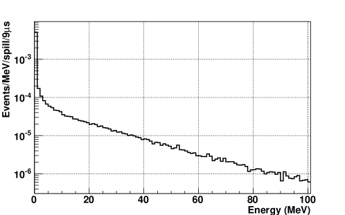
To reduce Type-A, it is effective to make an anti-coincidence by detecting parent muons in a time window of 20s prior to the event trigger time (“charged-veto cut”) or decay electrons until after 9s (“Michel electron cut”). For Type-B, the background will be efficiently suppressed by rejecting events with an energy smaller than 15 MeV, because the end point energy of the 12B -decay is 13.4 MeV. The counting rate of the residual background after those cuts can be estimated by the Monte Carlo simulation based on the result of the study for the background with use of the 500 kg plastic scintillator [2]. Figure 24 shows the expected background spectrum after the charged-veto cut and the Michel-electron cut. Since the end-point energy of and the threshold energy of the 12C(,eN reactions are 52.8 MeV and 17.3 MeV, respectively, the energy window for 12C(,eN is to be set between 20 MeV and 40 MeV, taking into account the energy resolution of the JSNS2 detector. The detection efficiencies with the energy window and the time window are determined with the Monte Carlo calculation as 67.4 and 74, respectively, and the expected counting rate of the 12C(,eN reaction is 1513 events/5000h/MW/50t. On the other hand, the background rate in this energy window is estimated to be 2.43105 events/5000h/MW, being two orders of magnitude larger than the expected counting rate of the 12C(,eN reaction.
Further reduction of the background will be achieved with the delayed coincidence of the 12N -decay. Considering the Q-value (17.4 MeV) of the 12N -decay and the ray background rate below 8 MeV, we will set the energy window from 10 MeV to 18 MeV for the delayed signal. To avoid the beam-related background, the beginning of the time window will be set at 0.1 ms from the rising edge of the proton beam pulse. On the other hand, the end of the time window will be set at 47.5 ms, which corresponds to three as long as the half-life (15.83 ms) of 12N, in order to acquire most of the positrons from 12N. The expected counting rates of and for the 12C(,eN signal and the background due to the accidental coincidence, respectively, are given by the following equations;
| (1) |
where , and are the number of target 12C nuclei, the flux of , and the cross section for the 12C(,eN reaction, respectively. and are the background rates for the prompt and the delayed signals, respectively. denotes the width of the time window for the coincidence between the prompt and the delayed signals. As mentioned above, the background rate in the prompt signal window is estimated as 2.43105 events/5000h/MW/50t.
From our previous study, the backgrounds in those windows are considered to be dominated by the cosmic-ray induced rays and neutrons. Therefore can be estimated by integrating the energy spectrum shown by Fig. 24 in the energy region for the delayed signal. The probability of the accidental coincidence is calculated as 2.3 /47.5ms/MW/50t from the estimated , suggesting still further reduction of the background is necessary. Since the background events are not correlated with the prompt signals from the 12C(,eN reaction, they can be reduced by careful analysises on spatial and time correlations between the prompt and the delayed signals.
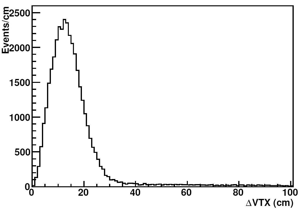
Figure 25 shows the distribution of ,
which is defined as the distance between the mean positions of
the prompt electron from 12C(,eN and the
delayed positron from 12N -decay estimated from
the distributions of the photons detected with PMTs.
Setting the criterion 20 cm, 82 of the
12C(,eN events are picked up, while the
background rate can be suppressed with a factor of 0.0011,
which is basically determined by the ratio of the whole volume
of the detector to the volume of a sphere with a radius of 20 cm.
Concerning the time correlation, the event rates of the prompt
electron and the delayed positrons are governed by the decays
with half-lives of 3.17 s and 15.83 ms, respectively, with
respective to the primary beam pulse. The 65 fraction of the random
background can be eliminated by the likelihood analysis on
the time distributions of the prompt and delayed signals
(“lifetime cut”: the similar cut as mentioned in Ref [2]).
On the other hand, according to our previous
simulation, 91 of the 12C(,eN events
will be kept.
The efficiencies and the rejection factors of the above cuts are summarized in Table 3.
| Cut | Efficiency | Rejection factor |
|---|---|---|
| Energy window (prompt 20-40MeV) | 0.674 | — |
| Time window (prompt 1-10s) | 0.74 | — |
| Energy window (delayed 10-18MeV) | 0.42 | — |
| Time window (delayed 0.1-47.5ms) | 0.944 | — |
| VTX cut | 0.82 | 0.0011 |
| Lifetime cut | 0.91 | 0.45 |
| total | 0.148 | 4.9510-4 |
Here it should be noted that the contribution of 12C(,eN∗ can be eliminated by requiring the delayed coincidence of the 12N -decay, because all the known excited states of 12N are located above the threshold of the proton emission.
Assuming the flux of to be 1.61014 /cm2/y/MW and the 12C(,eNg.s. cross section to be 8.910-42 cm2, the expected numbers of the events are estimated with the total efficiency and the total rejection factor in Table 3 as 448 /y and 138 /y for the 12C(,eNg.s. reaction and the background, respectively, with the total detector mass of 50 t and the operation of J-PARC/MLF at 1 MW for 5000 h/y, leading to a very good statistical accuracy of 6.0 (2.7) with a one- (five-) year measurement.
Systematic errors
In this measurement, major sources of the systematic error are supposed to be the uncertainties associating the absolute flux of incident neutrinos and the detector response. In the previous experiments by the KARMEN [40] and the LSND [36] collaborations, the neutrino fluxes were estimated by means of Monte Carlo simulations using the experimentally determined ratios of or to the incident protons, and the uncertainties in the neutrino fluxes were not smaller than 7, being greater than statistical errors of those experiments. A more accurate determination of the neutrino flux may be achieved by directly measuring the rates of the d(,e-p)p and d(,n)p reactions, whose cross sections are known with accuracy of 2 [41]. This kind of measurement will need an additional deuterated liquid scintillation counter located near the spallation target of J-PARC/MLF. For precise understanding of the detector response, we will develop movable sources in the active volume for calibrations of the position and energy measurements.
Determination of 12C(,eN∗ cross sections
To determine the cross section for 12C(,eN∗, the spectrum obtained for null delayed signal should be deconvoluted with the response functions for possible reaction channels such as 12C(,eN∗, 13C(,e-)X and 12C(,eNg.s with missing delayed signal. Due to more statistics than previous experiments and precise calibration of the detector response, better accuracy in the analysis of the angular distribution is expected.
Possibility for cross section measurements on neutrino-induced reactions other than 12C(,e-)12N
As mentioned above, an accurate measurement of a neutrino-induced reaction cross section requires a target mass of around one ton or more and a very low background rate. From the viewpoint of the target mass, 12C(C∗ and 13C(,e-)13N are the candidates, but unfortunately, there is no useful decay in both reactions for the delayed coincidence, and therefore thick passive shields should be added to suppress the background due to cosmic-ray induced -rays and neutrons. Another candidate will be the 28Si(,e-)28P reaction followed by the -decay of 28P with a Q-value of 14.35 MeV and a half-life of 270.3 ms. In this case the material for the liquid scintillator has to be replaced with a silicon compound such as silicon oil, and it should be regarded as one of the future extensions of JSNS2 after completion of the sterile neutrino search.
References
- [1] M.Harada, et al, arXiv:1310.1437 [physics.ins-det]
-
[2]
M.Harada, et al, arXiv:1502.02255 [physics.ins-det]
PTEP 2015 6, 063C01 (2015) - [3] M.Harada, et al, arXiv:1507.07076 [physics.ins-det]
- [4] M. Harada, et al., Settlement of Materials and Life Science Experimental Facility at J-PARC, Nucl. Inst. Meth, A600 (2009) 87–90.
- [5] Y. Ding, et al, Nucl. Instrum. Meth. A584, 238 (2008).
- [6] S. Agostinelli et al., Nucl. Instr. Meth. A 506, 250 (2003).
- [7] I .Shimizu, PhD thesis, Tohoku University (2004).
- [8] Y. Sakemi et al, IAEA-TECDOC-1743, 229 (2014).
- [9] J. Beringer et al. [Particle Data Group], Phys. Rev. D 86, 010001 (2012).
- [10] J. Spitz, Phys. Rev. D 85, 093020 (2012).
- [11] J. Spitz, Phys. Rev. D 89, 073007 (2014).
- [12] S. Axani, G. Collin, J.M. Conrad, M.H. Shaevitz, J. Spitz, and T. Wongjirad, Phys. Rev. D 92, 092010 (2015).
- [13] C. Rott, S. In, J. Kumar, and D. Yaylali, Journal of Cosmology and Astroparticle Physics 11, 039 (2015).
- [14] J-PARC Project Newsletter special issue, May 2015.
- [15] N.V. Mokhov, FERMILAB-FN-628 (1995); O.E. Krivosheev and N.V. Mokhov, “MARS Code Status”, Fermilab-Conf-00/181 (2000); O.E. Krivosheev and N.V. Mokhov, “Status of MARS Code”, Fermilab-Conf-03/053 (2003); N.V. Mokhov, K.K. Gudima, C.C. James et al., “Recent Enhancements to the MARS15 Code”, Fermilab-Conf-04/053 (2004).
- [16] T. Katori, Neutrino Cross Section Newsletter (12/23/2014); https://pprc.qmul.ac.uk/ katori/nu-xsec.html.
- [17] D. G. Michael et al. [MINOS Collaboration], Nucl. Instrum. Meth. A 596, 190 (2008).
- [18] D.S. Ayres et al. [NOvA Collaboration], FERMILAB-PROPOSAL-0929 (2004).
- [19] R. Acciarri et al., [DUNE Collaboration] (2015), Long Baseline Neutrino Facility (LBNF) and Deep Underground Neutrino Experiment (DUNE) Conceptual Design Report, available in 4 volumes at http://www.dunescience.org/.
- [20] K. Abe et al. [T2K Collaboration], Nucl. Instr. Meth. A 659, 106 (2011).
- [21] J. Cao et al., Phys. Rev. ST Accel. Beams 17, 090101 (2014).
- [22] E. Baussan et al., arXiv:1309.7022 [hep-ex] (2013).
- [23] J.E. Campagne, M. Maltoni, M. Mezzetto, and T. Schwetz, J. High Energy Phys. 0704, 003 (2007).
- [24] Private communication with N. Jachowicz.
- [25] V. Pandey, N. Jachowicz, T. Van Cuyck, J. Ryckebusch, and M. Martini, Phys. Rev. C 92, 024606 (2015).
- [26] S. Woosley and H.-T. Janka, Nat. Phys. 1, 147 (2005), and references therein.
- [27] A. Marek and H.-T. Janka, Astropys. J. 694, 664 (2009), and references therein.
- [28] K. Sumiyoshi and G. Roepke, Phys. Rev. C77, 055804 (2008).
- [29] H.-T. Janka and E. Mueller, Astron. Astropys. 306, 167 (1996).
- [30] K. Otsuki, H. Tagoshi, T. Kajino and S.Wanajo, Astrophys. J. 533, 424 (2000).
- [31] S. Wanajo, T. Kajino, G.J. Mathews and K. Otsuki, Astrophys. J. 554, 578 (2001).
- [32] T. Kajino, S. Wanajo and G.J. Mathews, Nucl. Phys. A704, 165c (2002).
- [33] T. Yoshida et al., Phys. Rev. Lett. 96, 091101 (2006).
- [34] S.X. Nakamura, K. Sumiyoshi and T. Sato, Phys. Rev. C80, 035802 (2009).
- [35] R. Maschuw (KARMEN Collab.), Prog. Part. Nucl. Phys. 40, 183 (1998).
- [36] L.B. Auerbach et al. (LSND Collab.), Phys. Rev. C64, 065501 (2001).
- [37] J.N. Abdurashitov et al. (SAGE Collab.), Phys. Rev. C59, 2246 (1999).
- [38] W. Hampel et al. (GALLEX Collab.), Phys. Lett. B420, 114 (1998); F. Kaether et al. (GALLEX Collab.), Phys. Lett. B685, 47 (2010).
- [39] J.R. Distel et al., Phys. Rev. C68, 054613 (2003).
- [40] R.L. Burman, M.E. Potter and E.S. Smith, Nucl. Instr. Meth. in Phys. Res. A291, 621 (1990).
- [41] S.X. Nakamura, K. Sumiyoshi, T. Sato, Phys. Rev. Lett. 98, 192501 (2007).