Sampling the isothermal-isobaric ensemble by Langevin dynamics

Abstract

We present a new method of conducting fully-flexible-cell molecular dynamics simulation in isothermal-isobaric ensemble based on Langevin equations of motion. The stochastic coupling to all particle and cell degrees of freedoms is introduced in a correct way, in the sense that the stationary configurational distribution is proved to be in consistent with that of the isothermal-isobaric ensemble. In order to apply the proposed method in computer simulations, a second order symmetric numerical integration scheme is developed by Trotter’s splitting of the single-step propagator. Moreover, a practical guide of choosing working parameters is suggested for user specified thermo- and baro-coupling time-scales. The method and software implementation are carefully validated by a numerical example.

I Introduction

Molecular dynamics (MD) simulation is a powerful tool for investigating a broad range of systems, from biological to materials sciences. In the equilibrium situation, it is of crucial importance to consider the ensemble that an MD simulation samples, because the quantities to observe are often calculated from the ensemble averages. Moreover, the equilibrium ensemble may serve as the initial condition for non-equilibrium MD simulations wang2014exploring . Most of early MD simulations solve the Hamiltonian dynamics, and sample the microcanonical ensemble. In practical applications, alternative ensembles like canonical or isothermal-isobaric (NPT) ensembles are usually more desirable, so various methods have been developed to sample the required ensemble by modifying the Hamiltonian dynamics.

One class of approaches to generate the desired ensemble is the extended phase space methods. For example, the Nosé-Hoover nose1984molecular ; hoover1985canonical , Nosé-Hoover chain martyna1992nose and stochastic Nosé-Hoover thermostats are proposed to generate the canonical ensemble; The Andersen andersen1980molecular , Parrinello-Rahman parrinello1981polymorphic ; parrinello1980crystal and Martyna-Tuckerman-Klein martyna1994constant ; martyna1996explicit barostats are proposed to generate the NPT ensemble. These methods share the idea of extending the physical phase-space (positions, velocities of particles and the simulation cell) by extra variables that control the temperature and/or pressure of the system. The dynamics of the extended system is carefully designed to fulfill the condition that if the trajectory is ergodic, then the marginal stationary distribution in the physical phase-space is consistent with that of the desired ensemble.

Langevin dynamics is an alternative method for generating the canonical ensemble. It has been proved that the ergodicity is guaranteed under mild restrictions mattingly2002ergodicity ; mattingly2002geometric , therefore the convergence to the canonical distribution is ensured in the limit of infinitely long simulation time. Because of this advantage, Langevin dynamics has attracted increasing attention recently, and various integration schemes were developed in order to improve the accuracy of numerical simulations bussi2007accurate ; melchionna2007design ; bou2010long ; leimkuhler2013robust ; leimkuhler2013rational ; gronbech2013simple ; peters2014stochastic . The first attempt of using the Langevin dynamics in generating the NPT ensemble was from Feller et.al. feller1995constant and Kolb and Dünweg kolb1999optimized , who proposed the Langevin dynamics for both the particle degrees of freedom and the volume of the simulation cell (isotropic cell fluctuation). These work are recently improved by Grønbech-Jensen and Farago gronbech2014constant and Di Pierro et. al. dipierro2015stochastic . Quigley and Probert coupled the Parrinello-Rahman dynamics with Langevin stochastic terms to extend the method to the fully flexible cell motions (anisotropic cell fluctuation) quigley2004langevin ; quigley2005constant . However, it is not possible, as the authors stated, to prove that the stationary distribution of the dynamics is subject to the NPT ensemble when the cell motion is stochastic and rotation-eliminated. Therefore, theoretically, the cell motions in this approach should be deterministic, and the convergence to the NPT distribution is not guaranteed, although the NPT distribution is one of the stationary distributions. In practice, the authors recommended to accept the cell stochastic motions at the cost of rigor in theory.

In this work, we propose a fully-flexible-cell NPT Langevin dynamics that allows explicit stochastic components in both the particle and cell motions, due to which the convergence of configurational distribution to the NPT ensemble is naturally ensured in the infinitely long time limit. We start by defining the Hamiltonian for an extended phase-space composed of scaled coordinates and simulation cell variables. Then the Langevin dynamics of this system can be directly written down, and the Boltzmann stationary distribution is obtained in the extended phase-space. In order to have a direct description of the particle motions in terms of physical coordinates, the scaled coordinates are transformed back, and the Langevin dynamics is reformulated accordingly by using Ito’s formula. The configurational stationary distribution is then proved to be consistent with that of the NPT ensemble by transforming the Boltzmann distribution back to the physical coordinates in the same way. To develop the numerical scheme, we start by considering the Fokker-Planck equation that is equivalent to the Langevin equation, then the scheme is formulated by splitting the single-step propagator of the Fokker-Planck equation according to Trotter’s theorem. By construction, the proposed scheme is of second order accuracy with respect to the time-step size.

Before moving to the main results of this work, it should be noted that it is in general difficult to check if the convergence to the NPT distribution is achieved in a finite simulation time. One might check the convergence of some properties of the system, for example the free energy profile along a certain reaction coordinate kelly2004calculation , but the choice of indicating properties depends on the nature of the system and what is wanted from the simulation, and they are usually not sufficient to prove the convergence of the distribution. Therefore, we do NOT intend to investigate the ergodicity or the speed of convergence to the desired ensemble distribution in numerical simulations. The significance of this work is to propose a new fully-flexible-cell NPT Langevin dynamics that takes the theoretical advantage of ergodicity, and can be used as an alternative to the existing NPT simulation methods.

This paper is organized as follows: The development of NPT Langevin dynamics is discussed in detail in Sec. II. The discretization of Langevin dynamics is provided in Sec. III. In Sec. IV, we validate the NPT Langevin dynamics by a solid argon system of triclinic region cell. This work is concluded in Sec. V.

II The Langevin equations of motion

We denote the particle positions in the system by $r_{1},\cdots,r_{N}$, where $N$ is the number of particles in the system. The simulation cell matrix is denoted by $h=[h_{1},h_{2},h_{3}]$, where $h_{\alpha},\alpha=1,2,3$ are cell vectors. The scaled (direct) coordinate of a particle $s_{i}$ is defined by $r_{i}=hs_{i}$. In order to generate the fully-flexible-cell NPT ensemble, all components of the cell vectors are allowed to fluctuate. We define the kinetic energy of the system by

$$K=\sum_{i}\frac{1}{2}m_{i}(h\dot{s}_{i})^{2}+\sum_{{\alpha\beta}}\frac{1}{2}M_{{\alpha\beta}}\dot{h}_{{\alpha\beta}}^{2},$$ (1)

where $M_{\alpha\beta}$ is the fictitious mass corresponding to the motion of $h_{\alpha\beta}$ that is the $\beta$-th component of the $\alpha$-th cell vector. The first term on the RHS of (1) is different from the physical kinetic energy of the system, which is $\sum\frac{1}{2}m_{i}[d(hs_{i})/dt]^{2}$. The consequence of this difference will be discussed in detail later. It is worth noting that the Parrinello-Rahman barostat parrinello1980crystal ; parrinello1981polymorphic also uses Eq. (1) as the definition of kinetic energy. The Lagrangian of the system is defined as

$$\mathcal{L}(\{s_{i}\},\{\dot{s}_{i}\},h,\dot{h})=K-(U+P\det(h)+{\chi{k_{{}_{\textrm{B}}}T}\ln[\det(h)]}),$$ (2)

where $U=U(hs_{1},\cdots,hs_{N})$ is the potential energy of the system, $P$ is the target pressure, $\chi$ is a constant that depends only on the dimension of the system and will be discussed in Remark 1, $T$ is the target temperature and $k_{B}$ is the Boltzmann constant . The generalized momenta corresponding to $r_{i}$ and $h$ are

$$\pi_{i}=m_{i}h^{\top}h\dot{s}_{i},\quad p^{h}_{\alpha\beta}=M_{\alpha\beta}\dot{h}_{\alpha\beta},$$ (3)

respectively. Therefore, the Hamiltonian of the system yields

$$\mathcal{H}(\{s_{i}\},\{\pi_{i}\},h,p_{h})=\sum_{{\alpha\beta}}\frac{(p^{h}_{\alpha\beta})^{2}}{2M_{\alpha\beta}}+\sum_{i}\frac{(h^{-\top}\pi_{i})^{2}}{2m_{i}}+U+P\det(h)+{\chi{k_{{}_{\textrm{B}}}T}\ln[\det(h)]}.$$ (4)

The first term on the RHS of (4) is the kinetic energy of cell vectors, and the summation of the last three terms gives the instantaneous enthalpy. The Langevin dynamics is defined by

$$\dot{s}_{i} =\frac{\partial\mathcal{H}}{\partial\pi_{i}}$$ (5a)

$$\dot{\pi}_{i} =-\frac{\partial\mathcal{H}}{\partial s_{i}}-\Gamma_{i}\frac{\partial\mathcal{H}}{\partial\pi_{i}}+\Sigma_{i}\dot{W_{i}}$$ (5b)

$$\dot{h}_{{\alpha\beta}} =\frac{\partial\mathcal{H}}{\partial p^{h}_{{\alpha\beta}}}$$ (5c)

$$\dot{p}^{h}_{{\alpha\beta}} =-\frac{\partial\mathcal{H}}{\partial h_{{\alpha\beta}}}-\hat{\gamma}_{{\alpha\beta}}\frac{\partial\mathcal{H}}{\partial p^{h}_{{\alpha\beta}}}+\hat{\sigma}_{{\alpha\beta}}\dot{W}_{\alpha\beta},$$ (5d)

where $W_{i}$, $W_{\alpha\beta}$ denote the standard Wiener processes, which are independent for different particle and cell degrees of freedom. The friction $\Gamma_{i}$ and noise magnitude $\Sigma_{i}$ are $h$ dependent matrices defined by $\Gamma_{i}=\gamma m_{i}h^{\top}h$, $\Sigma_{i}=\sigma\sqrt{m_{i}}\,h^{\top}$, where $\sigma^{2}=2\gamma{k_{{}_{\textrm{B}}}T}$, then the fluctuation-dissipation theorem $\Sigma_{i}\Sigma_{i}^{\top}=2\Gamma_{i}{k_{{}_{\textrm{B}}}T}$ holds for (5a)–(5b). We define $\hat{\gamma}_{\alpha\beta}=M_{\alpha\beta}\gamma_{\alpha\beta}$ and $\hat{\sigma}_{\alpha\beta}=\sqrt{M_{\alpha\beta}}\sigma_{\alpha\beta}$, where $\sigma^{2}_{\alpha\beta}=2\gamma_{\alpha\beta}{k_{{}_{\textrm{B}}}T}$, then the fluctuation-dissipation theorem $\hat{\sigma}_{\alpha\beta}^{2}=2\hat{\gamma}_{\alpha\beta}{k_{{}_{\textrm{B}}}T}$ holds for (5c)–(5d). It is well known that the stationary probability density of the Langevin dynamics (5) is

$$\rho_{\mathrm{equi}}\propto\exp\Big{[}-\frac{1}{{k_{{}_{\textrm{B}}}T}}\mathcal{H}(\{s_{i}\},\{\pi_{i}\},h,p^{h})\Big{]}.$$ (6)

It is more convenient to represent the Langevin dynamics (5) in physical coordinates, so we introduce the following transformation

$$r_{i}=hs_{i},\quad p_{i}=h^{-\top}\pi_{i}.$$ (7)

By using Ito’s formula, and writing down all partial derivatives explicitly, we reach

$$\dot{r}_{i} =\frac{1}{m_{i}}p_{i}+\dot{h}h^{-1}r_{i}$$ (8a)

$$\dot{p}_{i} =-\partial_{i}U-h^{-\top}\dot{h}^{\top}p_{i}-\gamma\,p_{i}+\sqrt{m_{i}}\,\sigma\,\dot{W}_{i}$$ (8b)

$$\dot{h}_{\alpha\beta} =\frac{1}{M_{\alpha\beta}}p^{h}_{\alpha\beta}$$ (8c)

$$\dot{p}^{h}_{\alpha\beta} =\det(h)\Big{[}\Big{(}P_{\textrm{ins}}-P-{\frac{\chi{k_{{}_{\textrm{B}}}T}}{\det(h)}}\Big{)}h^{-\top}\Big{]}_{\alpha\beta}-\gamma_{\alpha\beta}\,p^{h}_{\alpha\beta}+\sqrt{M_{\alpha\beta}}\,\sigma_{\alpha\beta}\,\dot{W}_{\alpha\beta},$$ (8d)

where $P_{\textrm{ins}}$ is the instantaneous pressure tensor defined by

$$P_{\textrm{ins}}=\frac{1}{\det(h)}\sum_{i}\Big{(}\frac{1}{m_{i}}p_{i}\otimes p_{i}+F_{i}\otimes r_{i}\Big{)}.$$ (9)

It can be easily shown that the Jacobian determinant of the transform (7) is 1, therefore, by integrating out the cell vector momenta, the equilibrium probability density generated by dynamics (8a)–(8d) is

$$\rho_{\mathrm{equi}}\propto{[\det(h)]^{-\chi}}\exp\Big{[}-\frac{1}{{k_{{}_{\textrm{B}}}T}}\Big{(}\sum_{i=1}^{N}\frac{p_{i}^{2}}{2m_{i}}+U(\{r_{i}\})+P\det(h)\Big{)}\Big{]}.$$ (10)

Remark 1: It was proposed by Ref. martyna1994constant that $\chi$ takes the value of $d-1$, where $d$ is the dimension of the system. If the rotation of the simulation cell is eliminated by taking $h$ as an upper (or lower) triangular matrix, then $\chi$ should take $(d-1)/2$ (see Appendix A for more details). The term $-\chi{k_{{}_{\textrm{B}}}T}/\det(h)$ on the RHS of Eq. (8d) can be effectively treated as a correction to the pressure difference $P_{\textrm{ins}}-P$, and vanishes under the thermodynamic limit, viz. the volume of the system $\det(h)$ goes to infinity.

Remark 2: It should be noted here that the particle momentum $p_{i}$ is not exactly the physical momentum $p^{\mathrm{phys}}_{i}$. As a matter of fact, we have the relation:

$$p^{\mathrm{phys}}_{i}=p_{i}+{m_{i}}\dot{h}h^{-1}r_{i}.$$ (11)

This inconsistency is the direct consequence of the definition of the kinetic energy (1), in which the particle contribution is not the physical kinetic energy. There is no substantial difficulty in using the physical definition, however, the derivation of the Langevin dynamics would become much more complicated. In most applications, only the correctness of system configuration is of importance. The current definition guarantees the configurational distribution to be consistent with that of the NPT ensemble. It is also worth noting that the particle momentum $p_{i}$ rather than $p^{\mathrm{phys}}_{i}$ should be used to estimate an equilibrium quantity that is an average over momentum-dependent instantaneous values (e.g. temperature and pressure). By using $p_{i}$, the equilibrium distribution (10) matches the form of the NPT distribution, so the average converges to the NPT equilibrium quantity under the infinity long time limit, and is independent with the parameters (frictions and the fictitious mass) in the Langevin dynamics.

Remark 3: The choice of the parameters in the Langevin dynamics (8) has been extensively discussed in literature, e.g. kolb1999optimized ; quigley2004langevin . We pick up the friction coefficients based on a rule of thumb quigley2004langevin : $\gamma=\gamma_{\alpha\beta}=\omega_{T}/2\pi=1/\tau_{T}$, where $\omega_{T}$ denotes the frequency of the thermostat and $\tau_{T}=2\pi/\omega_{T}$ is the time-scale of the thermostat. In order to provide the way of choosing the fictitious mass $M_{\alpha\beta}$, we firstly assume that the cell matrix $h$ is diagonal (a cuboid cell). With a first order expansion of the pressure with respect to the cell fluctuation in $h_{11}$, $h_{22}$ and $h_{33}$, we have

$$P-P^{0}=-\frac{1}{\kappa h^{0}_{11}h^{0}_{22}h^{0}_{33}}(h_{11}h_{22}h_{33}-h^{0}_{11}h^{0}_{22}h^{0}_{33}),$$ (12)

where $\kappa=-\frac{1}{V}\frac{\partial V}{\partial P}$ is the compressibility. The superscript “0” denotes the equilibrium value of the corresponding variable. We further assume that the fluctuation from the equilibrium value is small, i.e. $|h_{{\alpha\alpha}}-h_{{\alpha\alpha}}^{0}|,\ \alpha=1,2,3$ are small. Arranging the equation (12) in the component-wise way and preserving only the first order fluctuations on the RHS, we have

$$\frac{1}{3}\Big{[}(P_{11}-P_{11}^{0})+(P_{22}-P_{22}^{0})+(P_{33}-P_{33}^{0})\Big{]}\\ =-\frac{1}{\kappa h^{0}_{11}h^{0}_{22}h^{0}_{33}}\Big{[}(h_{11}-h^{0}_{11})h^{0}_{22}h^{0}_{33}+(h_{22}-h^{0}_{22})h^{0}_{11}h^{0}_{33}+(h_{33}-h^{0}_{33})h^{0}_{11}h^{0}_{22}\Big{]}.$$

One possible solution to the equation is

$$P_{{\alpha\alpha}}-P_{{\alpha\alpha}}^{0}=-\frac{3}{\kappa h^{0}_{{\alpha\alpha}}}(h_{{\alpha\alpha}}-h^{0}_{{\alpha\alpha}}),\quad\alpha=1,2,3.$$ (13)

By inserting (8c) and (13) into (8d), and discarding the friction and noise, $\chi$, and higher order terms, we have

$$M_{\alpha\alpha}\ddot{h}_{\alpha\alpha}=-\frac{3\det(h^{0})}{\kappa(h^{0}_{\alpha\alpha})^{2}}(h_{{\alpha\alpha}}-h^{0}_{{\alpha\alpha}}),$$

which is the equation of motion of harmonic oscillator $h_{{\alpha\alpha}}$ with spring constant $k_{\alpha\alpha}=\frac{3\det(h^{0})}{\kappa(h^{0}_{\alpha\alpha})^{2}}$ and equilibrium position $h_{{\alpha\alpha}}^{0}$. By using the relation $\omega_{\alpha\alpha}=\sqrt{k_{\alpha\alpha}/M_{\alpha\alpha}}$, where $\omega_{\alpha\alpha}$ is the barostat frequency, we derive the expression for the fictitious mass

$$M_{\alpha\alpha}=\frac{3\det(h^{0})}{\kappa(h^{0}_{\alpha\alpha})^{2}}\Big{(}\frac{1}{\omega_{\alpha\alpha}}\Big{)}^{2}=\frac{3\det(h^{0})}{\kappa(h^{0}_{\alpha\alpha})^{2}}\Big{(}\frac{\tau_{\alpha\alpha}}{2\pi}\Big{)}^{2},$$ (14)

where $\tau_{\alpha\alpha}$ is the time-scale of the barostat. For simplicity, we choose the off-diagonal value of fictitious mass by

$$M_{\alpha\beta}=\frac{3\det(h^{0})}{\kappa(h^{0}_{\alpha\alpha})^{2}}\Big{(}\frac{\tau_{\alpha\beta}}{2\pi}\Big{)}^{2}.$$ (15)

In practice, it is often impossible to predict the equilibrium cell matrix $h^{0}$ before performing the simulation, however, if the initial condition does not deviate very far from equilibrium, we take the initial value of $h$ as a reasonable guess for $h^{0}$. The compressibility $\kappa$ can either take an experimental value, or be estimated from short testing simulations using the formula: $\kappa=(\langle V^{2}\rangle-\langle V\rangle^{2})/({k_{{}_{\textrm{B}}}T}\langle V\rangle$).

It is worth noting that regardless of the choice of the parameters, the Langevin dynamics (8) samples the configurational distribution of the NPT ensemble at infinitely long time limit. The difference in using different parameters lies in the sampling efficiency. If the time-scales of the thermo- and barostat were chosen too large, then the temperature and pressure of the system would not be adjusted in a responsive way, and the sampling of the NPT ensemble would be too slow. On the other hand, if they were chosen too small, then an unnecessarily small time-step would be needed to keep the MD simulation stable. Therefore, it was suggested that the inverse time-scales be chosen just below the typical molecular frequency kolb1999optimized .

III Discretize the Langevin dynamics

The evolution of a system governed by the Langevin dynamics (8a) – (8d) is equivalently described by the following Fokker-Planck equation:

$$\frac{\partial\rho}{\partial t}=\mathcal{F}\rho,$$ (16)

where $\rho(t,\{r_{i}\},\{p_{i}\},h,p^{h})$ is the time dependent probability density defined on the phase space. $\mathcal{F}$ is the infinitesimal generator, which can be factorized as

$$\mathcal{F}=\mathcal{F}_{K}+\mathcal{F}_{U}+\mathcal{F}_{O}+\mathcal{F}^{h}_{K}+\mathcal{F}^{h}_{U}+\mathcal{F}^{h}_{O},$$ (17)

with each term defined by

$$\mathcal{F}_{K} =\sum_{i}\Big{[}\frac{p_{i}}{m_{i}}+\dot{h}h^{-1}r_{i}\Big{]}\cdot\frac{\partial}{\partial r_{i}}$$

$$\mathcal{F}_{U} =\sum_{i}\Big{[}-\partial_{i}U-h^{-\top}\dot{h}^{\top}p_{i}\Big{]}\cdot\frac{\partial}{\partial p_{i}}$$

$$\mathcal{F}_{O} =\sum_{i=1}^{N}\Big{[}\,3\gamma+\gamma p_{i}\frac{\partial}{\partial p_{i}}+\frac{m_{i}\sigma^{2}}{2}\frac{\partial^{2}}{\partial p_{i}^{2}}\,\Big{]}$$

$$\mathcal{F}^{h}_{K} =\sum_{\alpha\beta}\frac{p^{h}_{\alpha\beta}}{M_{\alpha\beta}}\frac{\partial}{\partial h_{\alpha\beta}}$$

$$\mathcal{F}^{h}_{U} =\sum_{\alpha\beta}\Big{\{}\det(h)\Big{[}\Big{(}P_{\textrm{ins}}-P-{\frac{\chi{k_{{}_{\textrm{B}}}T}}{\det(h)}}\Big{)}h^{-\top}\Big{]}_{\alpha\beta}\Big{\}}\frac{\partial}{\partial p^{h}_{\alpha\beta}}$$

$$\mathcal{F}^{h}_{O} =\sum_{\alpha\beta}\Big{[}\,\gamma_{\alpha\beta}+\gamma_{\alpha\beta}p^{h}_{\alpha\beta}\frac{\partial}{\partial p^{h}_{\alpha\beta}}+\frac{M_{\alpha\beta}\sigma_{\alpha\beta}^{2}}{2}\frac{\partial^{2}}{\partial(p^{h}_{\alpha\beta})^{2}}\,\Big{]}.$$

Given this factorization, the single-step propagator $e^{\Delta t\mathcal{F}}$ ($\Delta t$ being the time-step) can be split by the Trotter theorem:

$$e^{\Delta t\mathcal{F}}=e^{\frac{\Delta t}{2}\mathcal{F}^{h}_{U}}e^{\frac{\Delta t}{2}\mathcal{F}_{U}}e^{\frac{\Delta t}{2}\mathcal{F}^{h}_{K}}e^{\frac{\Delta t}{2}\mathcal{F}_{K}}e^{{\Delta t}\mathcal{F}^{h}_{O}}e^{{\Delta t}\mathcal{F}_{O}}e^{\frac{\Delta t}{2}\mathcal{F}_{K}}e^{\frac{\Delta t}{2}\mathcal{F}^{h}_{K}}e^{\frac{\Delta t}{2}\mathcal{F}_{U}}e^{\frac{\Delta t}{2}\mathcal{F}^{h}_{U}}+\mathcal{O}(\Delta t^{3}).$$ (18)

This style of splitting is actually the “BAOAB” scheme proposed by Ref. leimkuhler2013robust . The authors argued that the BAOAB splitting is more accurate than other schemes in the sense of configurational sampling. The action of propagator $e^{{\Delta t}\mathcal{F}_{K}}$ and $e^{{\Delta t}\mathcal{F}_{U}}$ corresponds to evolve $r_{i}$ and $p_{i}$ by $\Delta t$ under the ordinary differential equation $\dot{r}_{i}=\frac{1}{m_{i}}p_{i}+\dot{h}h^{-1}r_{i}$ and $\dot{p}_{i}=-\partial_{i}U-h^{-\top}\dot{h}^{\top}p_{i}$, respectively. Here we adopt the convention that the cell matrix $h$ is an upper triangular matrix, then one has to solve, in general, $\dot{x}=b+Ax$ with $A$ being an upper or lower triangular matrix. In the current work, the analytic solution of $\dot{x}=b+Ax$ in the upper and lower triangular cases are denoted by $x(t)=S_{u}(x(0),t,b,A)$ and $x(t)=S_{l}(x(0),t,b,A)$, respectively. The explicit forms of function $S_{u}$ and $S_{l}$ are provided in Appendix B. The action of propagator $e^{{\Delta t}\mathcal{F}_{O}}$ and $e^{{\Delta t}\mathcal{F}^{h}_{O}}$ corresponds to evolve variables $p_{i}$ and $p^{h}_{\alpha\beta}$ by $\Delta t$ under the Ornstein-Uhlenbeck process. In general, an Ornstein-Uhlenbeck process $dp=-\gamma pdt+\sigma\sqrt{m}dw_{t}$ can be explicitly solved by $p(t)=e^{-\gamma t}p(0)+\frac{\sigma}{\sqrt{2\gamma}}\sqrt{1-e^{-2\gamma t}}\sqrt{m}R$, where $R$ is a random number subject to the normal distribution with vanishing mean and unit variance, i.e. $\mathcal{N}(0,1)$.

Discarding the higher order terms and applying from left to right the propagators on the RHS of (18) yields the following numerical scheme:

1:while MD continues do

2:     $p^{h}_{\alpha\beta}\leftarrow p^{h}_{\alpha\beta}+{\Delta t}/2\,\det(h)[(P_{\textrm{ins}}-P-{\chi{k_{{}_{\textrm{B}}}T}}/{\det(h)})h^{-\top}]_{\alpha\beta}$

3:     $p_{i}\leftarrow S_{l}(p_{i},{\Delta t}/2,-\partial_{i}U,-h^{-\top}\dot{h}^{\top})$

4:     $h_{\alpha\beta}\leftarrow h_{\alpha\beta}+{\Delta t}/2\,({p^{h}_{\alpha\beta}}/{M_{\alpha\beta}}$)

5:     $r_{i}\leftarrow S_{u}(r_{i},{\Delta t}/2,{p_{i}}/{m_{i}},\dot{h}h^{-1})$

6:     $p^{h}_{\alpha\beta}\leftarrow e^{-\gamma_{\alpha\beta}{\Delta t}}p^{h}_{\alpha\beta}+\sqrt{1-e^{-2\gamma_{\alpha\beta}\Delta t}}\>\sqrt{M_{\alpha\beta}{k_{{}_{\textrm{B}}}T}}\,R$

7:     $p_{i}\leftarrow e^{-\gamma\Delta t}p_{i}+\sqrt{1-e^{-2\gamma\Delta t}}\>\sqrt{m_{i}{k_{{}_{\textrm{B}}}T}}R$

8:     $r_{i}\leftarrow S_{u}(r_{i},{\Delta t}/2,{p_{i}}/{m_{i}},\dot{h}h^{-1})$

9:     $h_{\alpha\beta}\leftarrow h_{\alpha\beta}+{\Delta t}/2\,({p^{h}_{\alpha\beta}}/{M_{\alpha\beta}}$)

10:     Compute the force for each particle

11:     $p_{i}\leftarrow S_{l}(p_{i},{\Delta t}/2,-\partial_{i}U,-h^{-\top}\dot{h}^{\top})$

12:     Compute the instantaneous pressure tensor

13:     $p^{h}_{\alpha\beta}\leftarrow p^{h}_{\alpha\beta}+{\Delta t}/2\,\det(h)[(P_{\textrm{ins}}-P-{\chi{k_{{}_{\textrm{B}}}T}}/{\det(h)})h^{-\top}]_{\alpha\beta}$

14:end while

The operators $\mathcal{F}_{O}$ and $\mathcal{F}_{O}^{h}$ are mutable, therefore, lines 6 and 7 in the algorithm can be swapped.

IV Numerical results

The NPT Langevin method was implemented in the in-house molecular dynamics simulation package MOASP developed on infrastructure JASMIN mo2010jasmin . In order to validate the theory and the implementation, we tested a solid argon system modeled by the Lennard-Jones interaction:

$$U(r)=\frac{C_{12}}{r^{12}}-\frac{C_{6}}{r^{6}}+C,$$ (19)

where $r$ is the distance between a pair of particles. $C_{12}=2.71507\times 10^{-7}$ $\mathrm{kJ\>mol}^{-1}\mathrm{nm}^{-12}$ and $C_{6}=1.72685\times 10^{-4}$ $\mathrm{kJ\>mol}^{-1}\mathrm{nm}^{-6}$ are parameters taken from the CHARMM27 force field foloppe2000all ; mackerell2000all . $C$ is a shifting constant that ensures the continuity of energy at the cut-off. The cut-off radius was chosen to be 0.9 nm in all simulations. The neighbor list was build for particles that are at most 1.1 nm apart, and was updated every 20 time-steps. If not stated otherwise, the time-step of integration was chosen to be 0.001 ps.

Figure 1: The equilibration of the Lennard-Jones argon system toward 300 K and 40 kBar. The simulation starts from a perfect FCC configuration at 0 K, and lasts for 100 ps. The plots present the equilibration of temperature (upper plot) and pressure (lower plot) at the first 2 ps. The solid line uses a compressibility of $4.5\times 10^{-5}$ $\mathrm{Bar}^{-1}$, and the dashed line uses a compressibility of $0.8\times 10^{-5}$ $\mathrm{Bar}^{-1}$.

An initial configuration of perfect FCC crystal was prepared by extending the Bravais lattice cell of $|h_{1}|=|h_{2}|=|h_{3}|=1.825$ nm and $\alpha=\beta=\gamma=60^{\circ}$ by $30\times 20\times 20$ times along three cell vectors, respectively. Therefore, the system contained 12,000 atoms in total. An 100 ps equilibration simulation that used this configuration and zero initial velocities was conducted at 300 K and 40 kBar. The initial guess of the compressibility was $4.5\times 10^{-5}$ $\mathrm{Bar}^{-1}$ (which was actually a value taken from the liquid water under ambient condition). The time-scales of thermostat and barostat were set to 0.1 ps and 0.5 ps, respectively. The system was successfully equilibrated to the desired thermodynamic state within only 1 ps (the solid lines in Fig. 1), and the initial FCC solid structure was stable under this thermodynamic condition. The finial coordinates and velocities of atoms were recorded for productive simulations. The compressibility, $0.8\times 10^{-5}$ $\mathrm{Bar}^{-1}$, was estimated from this simulation, and was used for all following simulations. Since the initial guess of the compressibility was much larger than $0.8\times 10^{-5}$ $\mathrm{Bar}^{-1}$, the speed of equilibration was actually faster than the user specified thermo- and barostat time-scales. We conducted the equilibration again with the correct compressibility, and found that the speed of equilibration was roughly the same as the specified thermo- and barostat time-scales (the dashed lines in Fig. 1).

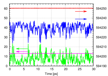
Figure 2: The conservation of Hamiltonian when the friction and noise vanish. The time evolution of the cell kinetic energy (green), $\chi{k_{{}_{\textrm{B}}}T}\ln[\det(h)]$ (pink), the instantaneous enthalpy (blue) and the Hamiltonian (red) are presented. The kinetic energy and $\chi{k_{{}_{\textrm{B}}}T}\ln[\det(h)]$ use the left y-axis, while the instantaneous enthalpy and the Hamiltonian use the right y-axis, as the arrows in the Figure indicate. The unit of the energy is kJ/mol.

An effective way to validate the correctness of the equations and software implementation is to check the conservation of Hamiltonian (4) when the friction and noise in (8) vanish. We performed this simulation with the initial positions and velocities from the previous equilibration, and plot the evolution of the cell kinetic energy, the instantaneous enthalpy, $\chi{k_{{}_{\textrm{B}}}T}\ln[\det(h)]$ and the Hamiltonian in Figure 2. A perfect conservation of the Hamiltonian is observed. It is worth mentioning that the cell kinetic energy and the instantaneous enthalpy fluctuate at the magnitude of roughly $\pm 5$ kJ/mol (see Fig. 2), and that the kinetic and potential energy of particles fluctuate at the magnitude of roughly $\pm 300$ kJ/mol (not shown).

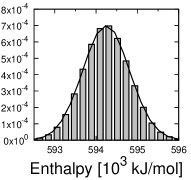
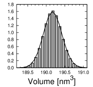
Figure 3: The distribution of the instantaneous enthalpy (left) and cell volume (right) of the solid argon system. The gray bars present the probability densities calculated from the 10,000 ps Langevin NPT simulation (this work) at 300 K and 40 kBar. The solid lines present the same probability densities calculated from the reference simulation (see the text for more details).

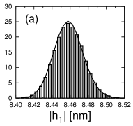
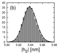
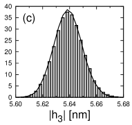
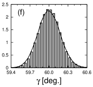
Figure 4: The distribution of cell vectors. Plot (a) – (c) on the left column present the probability densities of lengths of three cell vectors, i.e. $|h_{1}|$, $|h_{2}|$ and $|h_{3}|$, respectively. Plot (d) – (f) on the right column present the probability densities of three angles $\alpha$, $\beta$ and $\gamma$ between them, respectively. ($\alpha$ is the angle between $h_{2}$ and $h_{3}$. $\beta$ is the angle between $h_{1}$ and $h_{3}$. $\gamma$ is the angle between $h_{1}$ and $h_{2}$.) The simulated system is the same as Fig. 3.

Figure 5: The radial distribution functions calculated by the NPT Langevin (this work) and reference simulations. The two RDFs are plotted together in the upper plot; The difference between them is presented in the lower plot.

The productive NPT simulation lasted for 10,000 ps, and the data collection started from 100 ps. The instantaneous enthalpy and cell vectors were recorded every 0.02 ps. We plot the distribution of the instantaneous enthalpy and cell volume in Fig. 3. The distribution of the lengths of cell vectors and the angles between them are presented in Fig. 4. In the figures, the results of the NPT Langevin dynamics are compared and consistent with those of a reference simulation that uses velocity-rescaling thermostat bussi2007canonical and Parrinello-Rahman barostat parrinello1980crystal ; parrinello1981polymorphic . The initial condition and the other parameters were set to be the same as the Langevin simulation. The reference simulation is considered to be reliable, because it was conducted by a well-tested MD simulation package Gromacs hess2008gromacs ; pronk2013gromacs (version 4.6.5). The radial distribution functions (RDFs) calculated by Langevin and the reference simulation are shown to be overlapping in the upper plot of Fig. 5. From the lower plot of Fig. 5, we observe that the difference between them is dominated by the statistical uncertainty. This means that the solid structures sampled by Langevin dynamics reproduce those of the reference simulation.

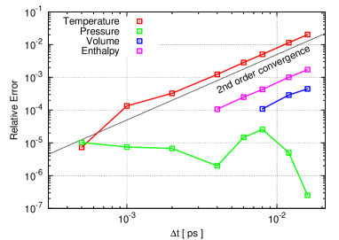
Figure 6: The convergence of temperature, pressure, volume and enthalpy with respect to the time-step ($\Delta t$) of the integration. The $x$-axis is the time-step in unit of picosecond, and the $y$-axis is the relative error. The reference values of the volume and enthalpy are obtain by the simulation using time-step 0.0005 ps. The relative errors of volume below $\Delta t$ = 0.008 ps and enthalpy below $\Delta t$ = 0.004 ps are dominated by statistical uncertainties, so they are not presented for clarity.

The NPT Langevin dynamics is numerically solved by the integration scheme in Sec. III that inevitably introduces error by time-discretization. To investigate its effect on temperature, pressure, volume and enthalpy computations, we present the relative errors vs. time-step size in a log-scaled plot (Fig. 6). The reference values of the volume and enthalpy are obtained by a simulation using the time-step of 0.0005 ps. The statistical uncertainty in estimating the relative errors are, on average, $4.7\times 10^{-5}$, $3.3\times 10^{-5}$, $1.1\times 10^{-4}$ and $1.0\times 10^{-4}$ (95% confidence level) for temperature, pressure, volume and enthalpy, respectively. The numerical results prove that the integration scheme is of second-order accuracy in computing the temperature, volume and enthalpy. The accuracy of pressure computation is remarkably high, so the errors are dominated by the statistical uncertainty ($3.3\times 10^{-5}$), and do not present the dependency on the time-step size. The relative errors in computing the cell vector lengths and angles are also dominated by the statistical uncertainty, and are not presented here.

V Conclusions and discussions

In this work, we proposed a new fully-flexible-cell Langevin dynamics in NPT ensemble. Our approach couples stochastic terms to both the particle and cell degrees of freedom, and is proved to correctly sample the configurational stationary distribution of the NPT ensemble. We noted that the choice of the working parameters (friction coefficients and the fictitious masses of cell vectors) does not affect the sampling of the NPT ensemble in the infinitely long time limit, however it determines the sampling efficiency and the size of the MD time-step. Therefore, we suggested a practical guide that automatically computes the fictitious mass and the friction coefficients by using the user specified thermo-/barostat time-scales, and the compressibility of the simulated material. In order to solve the Langevin equations by computers, a discretization scheme was developed by using the Trotter splitting of the single-step propagator of the Fokker-Planck equation. This scheme is, by construction, of second order accuracy. A solid argon system modeled by the Lennard-Jones interaction was simulated to validate the proposed Langevin dynamics and the numerical scheme. The conservation of the Hamiltonian in the case of vanishing friction and noise was firstly check, and the correctness of the equations and the software implementation was confirmed. Then the equilibrium distributions of enthalpy, cell volume and vectors were calculated, and were found to be in good consistency with those calculated by a reference simulation (conducted by package Gromacs 4.6.5). The accuracy of the equilibrium structure of the system was verified by comparing the radial distribution function with the reference simulation.

There are, roughly speaking, two classes of approaches for sampling canonical or isothermal-isobaric ensembles: The first is the deterministic approaches utilizing the extended phase space dynamics, while the second is the stochastic approaches introducing random noise in the dynamics. One can also find methods that combine the ideas from both classes of approaches, e.g. Ref. samoletov2007thermostats ; leimkuhler2009gentle ; dipierro2015stochastic . The main concern about the deterministic approaches is the ergodicity hoover1985canonical , the theoretical proof of which is, as far as we see, still unavailable. Thus the advantage of the stochastic approaches is the theoretically guaranteed ergodicity, which indicates that one can expect converged sampling of the desired ensemble in the infinitely long time limit. However, it should be noted that the theoretical proof of ergodicity does not necessarily ensure better performance in practice, because no real simulation is infinitely long. Both classes of approaches face the issue of how efficiently the phase space is explored. As discussed in Sec. I, this challenging question can be numerically investigated by checking the convergence of indicating properties on a case-by-case basis. As a matter of fact, one can find examples in the literature showing that the stochastic approaches are more precise in computing some properties (e.g. kelly2004calculation ), while other examples indicating that the deterministic approaches are more efficient (e.g. omelyan2013generalised ). Since it is impossible to derive a conclusive answer on which class of approaches is superior, we suggest to provide the users both options in MD simulation packages.

In this work, the numerical scheme for solving the Langevin equations is designed by a second order Trotter splitting of the single-step propagator. It worth mentioning that the proposed scheme is not the only possibility to achieve the time-discretization. Alternative schemes can be designed, for example, by manipulating the order of operators in Eq. (18) leimkuhler2013robust , or by minimizing the truncation errors of extended high-order splitting schemes with free parameters omelyan2002optimized ; omelyan2002optimized2 ; omelyan2003symplectic . The studies along this direction will be carried out in the future.

Although the Langevin dynamics is an efficient sampling tool of the equilibrium ensembles, the computed dynamical properties like time correlation functions are usually wrong, because the stochastic terms in the momentum equations break the physical dynamics of the system that is described by the Newton’s equations of motion. Therefore, in the cases where the dynamical properties are intended to be computed precisely, more carefully designed methods, e.g. local Langevin thermostat, should be used wang2015adaptive .

VI Acknowledgment

The authors acknowledge the valuable discussions with Aiqing Zhang, Xu Liu and Jianjun Liu, and the technical supports from them. H.W. thanks the fruitful discussions with Dr. Wei Zhang from Freie Universität Berlin. The authors gratefully acknowledge the financial support from National High Technology Research and Development Program of China under Grant 2015AA01A304. X.G. is supported by the National Science Foundation of China under Grants 91430218 and 61300012. H.W. is supported by the National Science Foundation of China under Grants 11501039 and 91530322.

Appendix A The value of constant $\chi$

In this section we follow the arguments of Ref. martyna1994constant . To separate the volume fluctuation from the total fluctuation of $h$, we let $h=V^{1/d}h_{0}$, where $V$ is the volume of the system, and $h_{0}$ with $\det(h_{0})=1$ accounts for the shape of the simulation cell. The partition function of the NPT ensemble (isotropic pressure control) reads

$$\Delta=\int dVdh_{0}\,e^{-{PV}/{k_{{}_{\textrm{B}}}T}}Q(V,h_{0})\,\delta(\det(h_{0})-1)$$ (20)

where $Q$ is the canonical partition function. When transforming $h_{0}$ back to $h$ in the integration, the measure transform $dh=(V^{1/d})^{d^{2}}dh_{0}$ is used for case that the $d^{2}$ components of the tensor $h$ are not constrained. If the rotation of $h_{0}$ (or equivalently $h$) is eliminated by taking $h_{0}$ as an upper triangular matrix ($(h_{0})_{\alpha\beta}=0,\ \alpha<\beta$), the number of degrees of freedoms in the tensor $h_{0}$ is $d(d+1)/2$, therefore we have the measure transform $dh=(V^{1/d})^{d(d+1)/2}dh_{0}$. In general, we denote $dh=(V^{1/d})^{\nu}dh_{0}$, and integrate the partition function Eq. (20) over $V$:

$$\Delta =\int dVdh\,V^{-\nu/d}\,e^{-{PV}/{k_{{}_{\textrm{B}}}T}}Q(h)\,V\delta(\det(h)-V)$$

$$=\int dh\,[\det(h)]^{-(\nu/d-1)}e^{-{P\det(h)}/{k_{{}_{\textrm{B}}}T}}Q(h).$$ (21)

This means the constant $\chi$ should take the value of $\nu/d-1$. When the simulation cell is allowed to rotate, $\nu=d^{2}$, so $\chi$ takes $d-1$. When the rotation of the simulation cell is removed, $\nu=d(d+1)/2$, so $\chi$ takes $(d-1)/2$.

Appendix B Solve the equation $\dot{x}=b+Ax$

The ordinary differential equation $\dot{x}=b+Ax$ can be solved analytically. We start with the case that $A$ is an upper triangular matrix:

$$\left[\begin{matrix}\dot{x}_{0}\\ \dot{x}_{1}\\ \dot{x}_{2}\end{matrix}\right]=\left[\begin{matrix}b_{0}\\ b_{1}\\ b_{2}\end{matrix}\right]+\left[\begin{matrix}a_{00}&a_{01}&a_{02}\\ 0&a_{11}&a_{12}\\ 0&0&a_{22}\\ \end{matrix}\right]\cdot\left[\begin{matrix}x_{0}\\ x_{1}\\ x_{2}\end{matrix}\right].$$ (22)

The solution is given by:

$$x_{0}(t)=\, x_{0}(0)e^{a_{00}t}+t\,b_{0}F_{1}(0,a_{00}t)$$

$$+t\,a_{01}x_{1}(0)F_{1}(a_{00}t,a_{11}t)+t^{2}\,a_{01}b_{1}F_{2}(a_{00}t,0,a_{11}t)$$

$$+t\,a_{02}x_{2}(0)F_{1}(a_{00}t,a_{22}t)+t^{2}\,a_{02}b_{2}F_{2}(a_{00}t,0,a_{22}t)$$

$$+t^{2}a_{01}a_{12}x_{2}(0)F_{2}(a_{00}t,a_{11}t,a_{22}t)+t^{3}a_{01}a_{12}b_{2}F_{3}(a_{00}t,a_{11}t,0,a_{22}t)$$ (23)

$$x_{1}(t)=\, x_{1}(0)e^{a_{11}t}+t\,b_{1}F_{1}(0,a_{11}t)$$

$$+t\,a_{12}x_{2}(0)F_{1}(a_{11}t,a_{22}t)+t^{2}\,a_{12}b_{2}F_{2}(a_{11}t,0,a_{22}t)$$ (24)

$$x_{2}(t)=\, x_{2}(0)e^{a_{22}t}+t\,b_{2}F_{1}(0,a_{22}t),$$ (25)

where the function $F_{1}$, $F_{2}$ and $F_{3}$ are defined to be

$$F_{1}(A,B) =\frac{e^{A}-e^{B}}{A-B}$$ (26)

$$F_{2}(A,B,C) =\frac{1}{B-C}(F_{1}(A,B)-F_{1}(A,C))$$ (27)

$$F_{3}(A,B,C,D) =\frac{1}{C-D}(F_{2}(A,B,C)-F_{2}(A,B,D)).$$ (28)

It should be noticed that the definitions have singularity when any two of the $A$, $B$, $C$ and $D$ are equal, and we do not exclude these cases in real simulations. Noticing that we only need the solution of (22) at small $t$, the singularity can be avoided by Taylor expansion of the exponential functions around 0. Following this idea, we reach the serial expansions of $F_{1}$, $F_{2}$ and $F_{3}$:

$$F_{1}(A,B) =\sum_{k=0}^{\infty}\frac{1}{(k+1)!}\sum_{\begin{subarray}{c}0\leq\alpha,\beta\leq k\\ \alpha+\beta=k\end{subarray}}A^{\alpha}B^{\beta}$$ (29)

$$F_{2}(A,B,C) =\sum_{k=0}^{\infty}\frac{1}{(k+2)!}\sum_{\begin{subarray}{c}0\leq\alpha,\beta,\gamma\leq k\\ \alpha+\beta+\gamma=k\end{subarray}}A^{\alpha}B^{\beta}$$ (30)

$$F_{3}(A,B,C,D) =\sum_{k=0}^{\infty}\frac{1}{(k+3)!}\sum_{\begin{subarray}{c}0\leq\alpha,\beta,\gamma,\delta\leq k\\ \alpha+\beta+\gamma+\delta=k\end{subarray}}A^{\alpha}B^{\beta}C^{\gamma}D^{\delta}.$$ (31)

For the case that $A$ is a lower triangular matrix:

$$\left[\begin{matrix}\dot{x}_{0}\\ \dot{x}_{1}\\ \dot{x}_{2}\end{matrix}\right]=\left[\begin{matrix}b_{0}\\ b_{1}\\ b_{2}\end{matrix}\right]+\left[\begin{matrix}a_{00}&0&0\\ a_{10}&a_{11}&0\\ a_{20}&a_{21}&a_{22}\\ \end{matrix}\right]\cdot\left[\begin{matrix}x_{0}\\ x_{1}\\ x_{2}\end{matrix}\right],$$ (32)

the solution can be written down in a similar way:

$$x_{0}(t)=\, x_{0}(0)e^{a_{00}t}+t\,b_{0}F_{1}(0,a_{00}t)$$ (33)

$$x_{1}(t)=\, x_{1}(0)e^{a_{11}t}+t\,b_{1}F_{1}(0,a_{11}t)$$

$$+t\,a_{10}x_{0}(0)F_{1}(a_{11}t,a_{00}t)+t^{2}\,a_{10}b_{0}F_{2}(a_{11}t,0,a_{00}t)$$ (34)

$$x_{2}(t)=\, x_{2}(0)e^{a_{22}t}+t\,b_{2}F_{1}(0,a_{22}t)$$

$$+t\,a_{21}x_{1}(0)F_{1}(a_{22}t,a_{11}t)+t^{2}\,a_{21}b_{1}F_{2}(a_{22}t,0,a_{11}t)$$

$$+t\,a_{20}x_{0}(0)F_{1}(a_{22}t,a_{00}t)+t^{2}\,a_{20}b_{0}F_{2}(a_{22}t,0,a_{00}t)$$

$$+t^{2}a_{21}a_{10}x_{0}(0)F_{2}(a_{22}t,a_{11}t,a_{00}t)+t^{3}a_{21}a_{10}b_{0}F_{3}(a_{22}t,a_{11}t,0,a_{00}t).$$ (35)

References

- (1) Han Wang, Christof Schuütte, Giovanni Ciccotti, and Luigi Delle Site. Exploring the conformational dynamics of alanine dipeptide in solution subjected to an external electric field: A nonequilibrium molecular dynamics simulation. Journal of Chemical Theory and Computation, 10(4):1376–1386, 2014.
- (2) S. Nosé. A molecular dynamics method for simulations in the canonical ensemble. Molecular Physics, 52(2):255–268, 1984.
- (3) W.G. Hoover. Canonical dynamics: Equilibrium phase-space distributions. Physical Review A, 31(3):1695–1697, 1985.
- (4) Glenn J Martyna, Michael L Klein, and Mark Tuckerman. Nosé–hoover chains: the canonical ensemble via continuous dynamics. The Journal of Chemical Physics, 97(4):2635–2643, 1992.
- (5) H.C. Andersen. Molecular dynamics simulations at constant pressure and/or temperature. The Journal of Chemical Physics, 72:2384, 1980.
- (6) M. Parrinello and A. Rahman. Polymorphic transitions in single crystals: A new molecular dynamics method. Journal of Applied Physics, 52:7182, 1981.
- (7) M. Parrinello and A. Rahman. Crystal structure and pair potentials: A molecular-dynamics study. Physical Review Letters, 45(14):1196–1199, 1980.
- (8) G.J. Martyna, D.J. Tobias, and M.L. Klein. Constant pressure molecular dynamics algorithms. The Journal of Chemical Physics, 101(5):4177–4189, 1994.
- (9) G.J. Martyna, M.E. Tuckerman, D.J. Tobias, and M.L. Klein. Explicit reversible integrators for extended systems dynamics. Molecular Physics, 87(5):1117–1157, 1996.
- (10) Jonathan C Mattingly, Andrew M Stuart, and Desmond J Higham. Ergodicity for sdes and approximations: locally lipschitz vector fields and degenerate noise. Stochastic Processes and Their Applications, 101(2):185–232, 2002.
- (11) Jonathan C Mattingly and Andrew M Stuart. Geometric ergodicity of some hypo-elliptic diffusions for particle motions. Markov Process. Related Fields, 8(2):199–214, 2002.
- (12) G. Bussi and M. Parrinello. Accurate sampling using langevin dynamics. Physical Review E, 75(5):056707, 2007.
- (13) S. Melchionna. Design of quasisymplectic propagators for langevin dynamics. The Journal of Chemical Physics, 127(4):44108–44108, 2007.
- (14) N. Bou-Rabee and H. Owhadi. Long-run accuracy of variational integrators in the stochastic context. SIAM Journal on Numerical Analysis, 48(1):278–297, 2010.
- (15) B. Leimkuhler and C. Matthews. Robust and efficient configurational molecular sampling via langevin dynamics. The Journal of Chemical Physics, 138:174102, 2013.
- (16) Benedict Leimkuhler and Charles Matthews. Rational construction of stochastic numerical methods for molecular sampling. Applied Mathematics Research eXpress, 2013(1):34–56, 2013.
- (17) Niels Grønbech-Jensen and Oded Farago. A simple and effective verlet-type algorithm for simulating langevin dynamics. Molecular Physics, 111(8):983–991, 2013.
- (18) Elias Alphonsus Jozef Franciscus Peters, Nicolae Goga, and Herman JC Berendsen. Stochastic dynamics with correct sampling for constrained systems. Journal of Chemical Theory and Computation, 10(10):4208–4220, 2014.
- (19) S.E. Feller, Zhang Y., R.W. Pastor, and B.R. Brooks. Constant pressure molecular dynamics simulation: the langevin piston method. The Journal of Chemical Physics, 103(11):4613–4621, 1995.
- (20) A Kolb and B Dünweg. Optimized constant pressure stochastic dynamics. The Journal of Chemical Physics, 111(10):4453–4459, 1999.
- (21) Niels Grønbech-Jensen and Oded Farago. Constant pressure and temperature discrete-time langevin molecular dynamics. The Journal of chemical physics, 141(19):194108, 2014.
- (22) Michele Di Pierro, Ron Elber, and Ben Leimkuhler. A stochastic algorithm for the isobaric-isothermal ensemble with ewald summations for all long range forces. Journal of Chemical Theory and Computation, 2015.
- (23) D Quigley and MIJ Probert. Langevin dynamics in constant pressure extended systems. The Journal of Chemical Physics, 120(24):11432–11441, 2004.
- (24) D Quigley and MIJ Probert. Constant pressure langevin dynamics: theory and application. Computer Physics Communications, 169(1):322–325, 2005.
- (25) Evan Kelly, Michael Seth, and Tom Ziegler. Calculation of free energy profiles for elementary bimolecular reactions by ab initio molecular dynamics: sampling methods and thermostat considerations. The Journal of Physical Chemistry A, 108(12):2167–2180, 2004.
- (26) Zeyao Mo, Aiqing Zhang, Xiaolin Cao, Qingkai Liu, Xiaowen Xu, Hengbin An, Wenbing Pei, and Shaoping Zhu. Jasmin: a parallel software infrastructure for scientific computing. Frontiers of Computer Science in China, 4(4):480–488, 2010.
- (27) Nicolas Foloppe and Alexander D MacKerell Jr. All-atom empirical force field for nucleic acids: I. parameter optimization based on small molecule and condensed phase macromolecular target data. Journal of Computational Chemistry, 21(2):86–104, 2000.
- (28) Alexander D Mackerell and Nilesh K Banavali. All-atom empirical force field for nucleic acids: Ii. application to molecular dynamics simulations of dna and rna in solution. Journal of Computational Chemistry, 21(2):105–120, 2000.
- (29) G. Bussi, D. Donadio, and M. Parrinello. Canonical sampling through velocity rescaling. The Journal of Chemical Physics, 126:014101, 2007.
- (30) B. Hess, C. Kutzner, D. van der Spoel, and E. Lindahl. Gromacs 4: Algorithms for highly efficient, load-balanced, and scalable molecular simulation. J. Chem. Theory Comput, 4(3):435–447, 2008.
- (31) S. Pronk, S. Páll, R. Schulz, P. Larsson, P. Bjelkmar, R. Apostolov, M.R. Shirts, J.C. Smith, P.M. Kasson, D. van der Spoel, B. Hess, and E. Lindahl. Gromacs 4.5: a high-throughput and highly parallel open source molecular simulation toolkit. Bioinformatics, page btt055, 2013.
- (32) Alex A Samoletov, Carl P Dettmann, and Mark AJ Chaplain. Thermostats for ”slow” configurational modes. Journal of Statistical Physics, 128(6):1321–1336, 2007.
- (33) B. Leimkuhler, E. Noorizadeh, and F. Theil. A gentle stochastic thermostat for molecular dynamics. Journal of Statistical Physics, 135(2):261–277, 2009.
- (34) Igor Omelyan and Andriy Kovalenko. Generalised canonical–isokinetic ensemble: speeding up multiscale molecular dynamics and coupling with 3d molecular theory of solvation. Molecular Simulation, 39(1):25–48, 2013.
- (35) IP Omelyan, IM Mryglod, and Reinhard Folk. Optimized verlet-like algorithms for molecular dynamics simulations. Physical Review E, 65(5):056706, 2002.
- (36) IP Omelyan, IM Mryglod, and Reinhard Folk. Optimized forest–ruth-and suzuki-like algorithms for integration of motion in many-body systems. Computer Physics Communications, 146(2):188–202, 2002.
- (37) IP Omelyan, IM Mryglod, and R Folk. Symplectic analytically integrable decomposition algorithms: classification, derivation, and application to molecular dynamics, quantum and celestial mechanics simulations. Computer Physics Communications, 151(3):272–314, 2003.
- (38) Han Wang and A. Agarwal. Adaptive resolution simulation in equilibrium and beyond. The European Physical Journal Special Topics, 224(12):2269–2287, 2015.